Heuristic algorithms for the Maximum Colorful Subtree problem

Abstract

In metabolomics, small molecules are structurally elucidated using tandem mass spectrometry (MS/MS); this resulted in the computational Maximum Colorful Subtree problem, which is NP-hard. Unfortunately, data from a single metabolite requires us to solve hundreds or thousands of instances of this problem; and in a single Liquid Chromatography MS/MS run, hundreds or thousands of metabolites are measured.

Here, we comprehensively evaluate the performance of several heuristic algorithms for the problem against an exact algorithm. We put particular emphasis on whether a heuristic is able to rank candidates such that the correct solution is ranked highly. We propose this “intermediate” evaluation because evaluating the approximating quality of heuristics is misleading: Even a slightly suboptimal solution can be structurally very different from the true solution. On the other hand, we cannot structurally evaluate against the ground truth, as this is unknown. We find that one particular heuristic consistently ranks the correct solution in a top position, allowing us to speed up computations about 100-fold. We also find that scores of the best heuristic solutions are very close to the optimal score; in contrast, the structure of the solutions can deviate significantly from the optimal structures.

1 Introduction

Metabolomics characterizes the collection of all metabolites in a biological cell, tissue, organ or organism using high-throughput techniques. Liquid Chromatography Mass Spectrometry (LC-MS) is one of the predominant experimental platforms for this task. Today, a major challenge is to determine the identities of the thousands of metabolites detected in one LC-MS run. This is also true for related fields such as natural products research [23], biomarker discovery, environmental science, or food science. Tandem mass spectrometry (MS/MS) is used to derive information about the metabolites’ structures. Interpretation of the hundreds to thousands of MS/MS spectra generated in a single LC-MS run remains a bottleneck in the analytical pipeline [23]. MS/MS data is usually searched against spectral libraries [19], but only a small number of metabolites (around 2 %) can be identified in this manner [7]. Recently, computational methods have been developed that do not search in spectral libraries but rather in molecular structure databases [5, 6, 2, 16, 22, 21, 9, 1, 18, 15]. CSI:FingerID [9] has won several competitions on the identification of small molecules from MS/MS data [17]; the web service for CSI:FingerID currently analyzes more than 2000 queries a day. At the heart of CSI:FingerID and its variants [5, 6] lies the computation of fragmentation trees, as these can be readily analyzed by kernel-based methods using multiple kernel learning [18].

Fragmentation trees were introduced in 2008 [4] and were initially targeted at the identification of the molecular formulas of small molecules; later, it was shown that the structure of fragmentation trees contains valuable information for structural elucidation of the underlying molecule [12, 13]. Computing an optimum fragmentation tree leads to the Maximum Colorful Subtree problem [4]. Unfortunately, this problem is NP-hard and also hard to approximate [14, 10]. Algorithms exist to solve the problem either heuristically [14] or exactly [4, 14, 24]. The problem is a variant of the well-studied Graph Motif problem [8, 11].

Approximation algorithms are algorithms for (usually) NP-hard problems with provable guarantees on the distance of the returned solution to the optimal one. But in bioinformatics research, the objective function is usually only a “crutch” used to find the optimum structure, whereas the value of the objective function has little or no meaning. To this end, heuristics in bioinformatics are designed to find solutions structurally similar to the optimum solution or, even better, the biological ground truth. This makes it intrinsically difficult to evaluate the performance of these heuristics, as we have to define a measure on the structural similarity between the heuristic solution and the biological ground truth; furthermore, the biological ground truth has to be known.

We will use an alternative way to evaluate the performance of a heuristic: For many applications, one biological instance results in a multitude of computational instances, corresponding to candidates or hypotheses; the score of the computational problem is used to rank these hypotheses. Although the ground truth may not be known for the structure of the best solution, we may have information regarding the correct candidate or hypothesis. To this end, we can evaluate a heuristic based on its ability to top-rank the correct candidate.

We propose several heuristics for the Maximum Colorful Subtree problem, and evaluate these heuristics with regards to their ranking quality. We find that one particular heuristic allows us to quickly confine the set of candidates (molecular formulas of the precursor molecule). This constitutes a filter, such that optimum solutions have to be sought only for a (preferably small) subset of candidates. We also evaluate whether the structure of the constructed solutions is similar to the optimum solution.

2 The Maximum Colorful Subtree problem

Let $G=(V,E)$ be a node-colored, rooted, directed acyclic graph (DAG) with root $r\in V$ and edge weights $w:E\to\mathbb{R}$. Let $C(G)$ be the set of colors used in $G$, and let $c(v)\in C(G)$ be the color assigned to node $v\in V$. We will consider subtrees $T=(V_{T},E_{T})$ of $G$ rooted at $r$. Let $C(T)$ be the set of colors used in $T$. We say that $T$ is colorful if all of its nodes have different colors.

The Maximum Colorful Subtree problem asks to find a colorful $r$-rooted subtree $T$ of $G$ of maximum weight, where $G$ is a DAG with node colors, edge weights and root $r\in V$. We may assume that $G$ is (weakly) connected and that $r$ is the unique source of $G$, as we can remove all nodes from the graph which cannot be reached by a path from the root $r$, without changing the optimal solution.

We note that previous work on the problem also makes the assumption of a single source, albeit usually implicitly [13, 4, 14, 24]. From an algorithmic standpoint, problem variants with or without a given root are “basically equivalent”: Given an algorithm that does not assume a fixed root $r$, we can solve an instance of the problem variant with root $r$ by introducing a superroot $r^{*}$ connected solely to $r$, sufficiently large edge weight $w(r^{*},r)$ and a new color for $r^{*}$. For the reverse direction, we solve the problem for every $r\in V$, then choose the best solution.

But there are two peculiarities when computing fragmentation trees that are different from the general problem, and that we will make use of here: First, any DAG used for fragmentation tree computation is transitive: That is, $uv\in E$ and $vw\in E$ implies $uw\in E$. Second, a coloring $c:V\to C(G)$ of DAG $G=(V,E)$ is order-preserving if there is an ordering ‘$\prec$’ on the colors $C(G)$ such that $c(u)\prec c(v)$ holds for every edge $uv$ of $G$ [10]. Computing fragmentation trees naturally results in order-preserving colors, as nodes can be colored by the fragment mass that is responsible for this node, and edges exist only between nodes from larger to smaller masses. The Maximum Colorful Arborescence problem [10] asks to find a colorful induced subtree $T$ of $G$ of maximum weight, where $G$ is a DAG with order-preserving colors and edge weights. See [10] for numerous complexity results. Here, we will stick with the name “Maximum Colorful Subtree problem”, but nevertheless assume that the coloring is order-preserving, unless indicated otherwise.

3 Heuristics for the Maximum Colorful Subtree problem

The following postprocessing methods can be applied to a tree $T=(V_{T},E_{T})$ after any heuristic: The Remove Dangling Edges (RDE) postprocessing iteratively removes edges $uv$ from $T$, where $v$ is a leaf and $w(uv)<0$; this is repeated until no more such edges are found. In contrast, the Remove Dangling Subtrees (RDS) postprocessing does not consider a single edge at a time, but rather induced subtrees: Each node $u\in V_{T}$ is scored by the maximum weight of any induced subtree rooted in $u$. Score $D[u]$ can be computed using dynamic programming:

$$D[u]=\sum\nolimits_{uv\in E_{T}}\max\{0,w(u,v)+D[v]\}$$

Clearly, $D[u]\geq 0$. For each edge $uv$ with $w(u,v)+D[v]<0$ we remove $uv$ and the subtree below it. Both postprocessings can be computed in $O(\left\lvert V_{T}\right\rvert)$ time using a tree traversal, as every edge is considered once and $\left\lvert E_{T}\right\rvert=\left\lvert V_{T}\right\rvert-1$. Figure 1 shows an example of the RDS postprocessing.

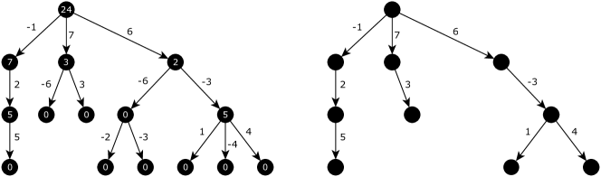
Figure 1: Illustration of the Remove Dangling Subtrees (RDS) postprocessing. Left: Input tree, where each node $v$ is labeled by its score $D[v]$. Right: Output tree of weight $24$.

We now present heuristics for finding a colorful subtree with root $r$ in a transitive DAG with order-preserving coloring and unique source $r$.

• Kruskal-style. This heuristic sorts all edges of the graph by decreasing edge weight, then iteratively adds edges from the sorted list, ensuring that the growing subgraph is colorful and that each node has at most one incoming edges. Since $r$ is the unique source of $G$, and since $G$ is transitive, this will ultimately result in a colorful subtree of $G$. This heuristic is similar to Kruskal’s algorithm for computing an optimum spanning tree; it was called “greedy heuristic” in [4].

• Prim-style. This heuristic progresses similar to Prim’s algorithm for calculating an optimal spanning tree: The tree $T=(V_{T},E_{T})$ initially contains only the root $r$ of $G$. In every step, we consider all edges $uv$ with $u\in V_{T}$ and $v\notin V_{T}$ such that $c(v)\notin C(V_{T})$; among these, we choose the edge with maximum weight and add it to the tree. We repeat until all colors in the graph are used in the tree. This will usually result in a different tree than the Kruskal-style heuristic, due to the colorfulness constraint.

• Insertion. This heuristic is a modification of the “insertion heuristic” from [14]. We again start with a tree $T=(V_{T},E_{T})$ containing only the root $r$ of $G$. The heuristic greedily attaches nodes labeled with unused colors. For every node $v$ with $c(v)=c^{\prime}$ unused, and every node $u$ already part of the solution, we calculate how much we gain by attaching $v$ to $u$. To calculate this gain, we take into account the score of the edge $uv$ as well as the possibility of rerouting other outgoing edges of $u$ through $v$:

  $$I(u,v):=w(uv)+\displaystyle\sum_{x\in V_{T},w(vx)>w(ux)}\bigl{(}w(vx)-w(ux)\bigr{)}$$

  where we assume $w(uv)=-\infty$ if $uv\notin E$. The node with maximum gain is then attached to the partial solution, and edges are rerouted as required. See [14] for details; different from there, we do not iterate over colors in some fixed order but instead, consider all unused colors in every step.

• Top-down. The top-down heuristic [4] is also greedy, but adds paths beginning in the root to the partial solution. The partial solution initially contains only the root $r$ of $G$. The heuristic greedily constructs a path starting at the root which is added to the partial solution; the next node of the path is chosen so that it maximizes the weight of the added edge, simultaneously ensuring that the partial solution remains colorful and does not violate the tree property. If no such edge exists, the algorithm restarts at the root, and searches for another path. It terminates if no edge at the root can be selected. In the resulting tree, all internal nodes but the root have exactly one child. This heuristic extends even simpler heuristics that attach all nodes to the root, which have been in frequent use for molecular formula determination from MS/MS data.

• Critical Path¹. Again, we iteratively build the subtree; initially, the partial solution $T$ contains only the root $r$ of $G$. The score $S[u]$ of a node $u\in V$ is the maximum weight of a path $p$ from $u$ to any node $v$, such that $C(p)\cap C(V_{T})\subseteq\{c(u)\}$; that is, the path does not use nodes with colors already present in the tree, except for the color of the starting node. We can compute $S[u]$ using the recurrence

  $$S[u]=\max\nolimits_{uv\in E,c(v)\notin C(V_{T})}\{0,\ S[v]+w(uv)\}$$ (1)

  where we use that the coloring of $G$ is order-preserving, since in that case no two nodes of the path have the same color. We further assume $\max\emptyset=0$ when computing (1). We iterate over the ordered colors in reverse order, computing $S[u]$ for all nodes $u$ of the active color. The critical path $p$ of maximum score can be found by backtracing from the maximum entry $S[u]$ with $u\in V_{T}$. We add $p$ to $T$, then iterate, recomputing $S$ for the new set of used colors $C(V_{t})$. See Figure 2 for an example.

  

  

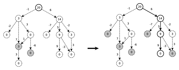
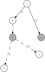
  Figure 2: Left: Example for the Critical Path Heuristic. Nodes are labeled by score, solid lines show the tree, dashed lines the rest of the graph. Grayed-out nodes have colors already used in the subtree. Right: An example input graph for which Critical Path¹ produces a better tree than Critical Path². Nodes $v$ and $z$ are the same color; all other nodes have distinct colors. The two solid edges are the suboptimal tree output by Critical Path². Critical Path¹ initially chooses the path $ruvx$ for a score of 6, then adds $vy$ for a total of 8. Critical Path² begins in the same way by choosing the first edge $ru$ of the heaviest path for a score of 2, but in its second step it chooses the weight-5 edge $rz$, as the heaviest path starting with $uv$ has weight 4. No further edges can be added, so the total weight is 7.

• Critical Path². This heuristic also relies on critical paths, but adds, in each iteration, only the first edge of the critical path to the partial solution. We note that this heuristic does not dominate the Critical Path heuristic, meaning that in certain cases, the subtree computed by this heuristic has smaller weight than that computed by the Critical Path heuristic; see Figure 2 (right) for an example.

• Critical Path³. This heuristic combines the Insertion heuristic with the Critical Path heuristic: In each step the heuristic chooses the edge $uv$ with $u\in V_{T}$ that maximizes the sum of critical path score and insertion score $S[u]+I(v)$.

• Maximum. All heuristics compute lower bounds of the maximum score; therefore the maximum score over all heuristic solutions is also a lower bound.

Time complexity of the heuristics.

Let $n:=\left\lvert V\right\rvert$, $m:=\left\lvert E\right\rvert$, and $k:=\left\lvert C(G)\right\rvert$. Clearly, $k\leq n$ and in applications, we usually have $k\ll n$. Furthermore, $\left\lvert V_{T}\right\rvert\leq k$ holds for the returned subtree $T=(V_{T},E_{T})$.

• It is easy to check that the Kruskal-style heuristic has time complexity $O(m\log n)$ for sorting all edges according to weight. Connectivity testing can then be performed in sub-logarithmic time per considered edge using a union-find data structure [20]; checking for colorfulness is easily accommodated by initially placing all nodes of the same color in the same component. The overall time complexity thus remains $O(m\log n)$. Similarly, the Prim-style heuristic requires $O(m\log n)$ time.

• For the Insertion heuristic, computing gain $I(u,v)$ for all $u$ requires $O(k^{2})$, since $u,x\in V_{T}$. Hence, attaching one $v$ to the growing tree requires $O(k^{2}n)$ time, resulting in $O(k^{3}n)$ total running time.

  But there exists a more complicated yet faster implementation for this heuristic: For each $v\in V$, we maintain two scores, $\mathit{in}(v)$ and $\mathit{out}(v)$, which correspond to the two terms on the RHS of the definition of $I(u,v)$. Specifically, $\mathit{in}(v)=\max_{u\in V_{T}}w(uv)$, and $\mathit{out}(v)=\sum_{x\in V_{T}}\max\{0,w(vx)-w(p_{T}(x),x)\}$, where $p_{T}(x)$ is the parent of $x$ in $T$ for all $x\in T$. To choose the next node to insert, we look for the node $v\in V$ maximizing $\mathit{in}(v)+\mathit{out}(v)$, ignoring nodes of already-used colors, which takes $O(n)$ time (and could in practice often finish early if we search in decreasing order of one of these terms, and know an upper bound on the other). We then perform a single $O(k)$-time scan to find its optimal parent in the tree, and then perform two further updates: First, for all $u\in V$, set $\mathit{in}(u)\leftarrow\max\{\mathit{in}(u),w(vu)\}$ and $\mathit{out}(u)\leftarrow\mathit{out}(u)+w(uv)-w(p_{T}(v),v)$. Second, for all $x\in V_{T}$, check whether the incoming edge $yx$ (i.e., $y=p_{T}(x)$) can be improved by rerouting via $v$; if so, delete $yx$, insert $vx$ and for all $u\in V$ such that $w(yx)\leq w(ux)$, set $\mathit{out}(u)\leftarrow\max\{0,\mathit{out}(u)-(w(vx)-w(yx))\}$. The second update needs $O(kn)$ time per inserted node, for $O(k^{2}n)$ overall.

• The Top-down heuristic searches at most $k$ times for the maximum weight edge leaving a node; since there are $O(n)$ such edges, the running time is $O(kn)$.

• For the Critical Path¹ heuristic, we need $O(m)$ time to compute values $S[u]$ and to identify the path of maximum weight. This is repeated at most $k-1$ times, resulting in a total running time of $O(km)$. The same holds true for the Critical Path². For Critical Path³ we can again maintain an $\mathit{out}(v)$ table that contains the score bonus we get for attaching a node in the intermediate tree as child of $v$ and deleting its previous incoming edge. After each insertion of an edge into the intermediate tree we have to perform the two update operations on $\mathit{out}$ which takes $O(kn)$ per insertion. In total we need $O(k^{2}n+km)$ time to compute Critical Path³. In applications, $k$ is very small and $n\ll m$, so the $O(km)$ part for calculating the critical paths requires most of the computation time.

Computing the $k$-best fragmentation trees exactly.

Even if we do not trust the structural quality of the heuristic solution, the above heuristics allow us to speed up fragmentation tree computation: We first select a single candidate (molecular formula of the precursor) using one of the heuristics, then compute the optimal solution for this instance using an exact method [4, 14, 24]. In practice, this approach has two shortcomings: Even though certain heuristics show a very good performance in selecting the correct molecular formula (see below), this correct answer is not known to us in application; but we will observe that the computed fragmentation tree will often not be the optimum fragmentation tree, if we also consider other molecular formula candidates and corresponding instances.

Even worse, it is usually not sufficient in application to select a single best candidate using the heuristic, then re-compute the fragmentation tree for the corresponding instance. Instead, we usually want to know optimal fragmentation trees for the $k$ best-scoring candidate. This is independent of whether results are reported to the user, who wants to use fragmentation tree structure to survey if computations and, hence, the assigned precursor molecular formula are trustworthy; or, if we perform some downstream computational analysis based on fragmentation tree structure, such as CSI:FingerID [9]. In particular for “large” metabolites with mass beyond 600 Dalton, this is necessary because neither the heuristics nor the exact method will always allow us to find the correct candidate; only by considering several candidates, we can be sufficiently sure that the correct answer is present.

We propose the following heuristic to compute optimum fragmentation trees for the $k$-best molecular formula candidates: First, we compute heuristic solutions for all candidates, and order molecular formula candidates according to the heuristic score. Next, we compute optimum fragmentation trees for the $k$ best candidates; for small $k$, we can instead choose some fixed parameter, such as 10 candidates. We estimate the maximum $\Delta\geq 0$ of differences between the score of the optimum solution and the corresponding heuristic solution, using those candidates where we know the exact solution. We now assume that the score difference is upper-bounded by $\Delta$ for all candidates. We continue to process candidates and compute optimum fragmentation trees from the sorted list, updating the $k$-best candidates and the corresponding score threshold; we stop computations when the heuristic score of a candidate plus $\Delta$ is smaller than the current score threshold. Clearly, our assumption made above may be violated for certain input, making this method a heuristic.

4 Data and Instances

Details of how to transform the MS/MS spectrum of an (unknown) compound into one or more instances of the Maximum Colorful Subtree problem have been published elsewhere [4, 3]; we shortly recapitulate the process. We consider all molecular formulas from some ground set, such as, all molecular formulas from elements CHNOPS. We decompose the precursor mass into all possible candidate molecular formulas from this ground set; each candidate molecular formula corresponds to one instance. For each instance, we decompose the fragment peaks in the MS/MS spectrum, ensuring that each fragment molecular formula is a subformula of the candidate molecular formula for the precursor mass. These molecular formulas constitute the nodes of a graph; each node is colored by the peak it stems from. An edge is present between molecular formulas $u,v$ if and only if $v$ is a proper subformula of $u$. Now, both nodes and edges receive a certain weight [3], based both on prior knowledge (e.g., distribution of loss masses) and the data (e.g., mass difference between a peak and its hypothetical molecular formula); but as pointed in [4], we may assume that only edges are weighted. Candidate molecular formulas of the precursor peak are ranked according to the weight of the maximum colorful subtree in this graph. SIRIUS 3.6 default weights are used, see [3].

To evaluate whether a heuristic is capable of ranking the correct molecular formula on the top position, we have to use reference data where the true compound structure is known for each MS/MS measurement. We use reference compounds from GNPS [23]; each reference compound is one instance, corresponding to several graphs (for the different molecular formula candidates of the precursor mass) we have to search in. We then filter instances: For example, we assume a mass accuracy of 10 ppm (parts per million), and discard compounds where the precursor mass is missing or outside outside this mass window. All details can be found in [3]. This leaves us with 4 050 compounds, each of which is then transferred to usually many instances of the Maximum Colorful Subtree problem. One reference compound resulted in between 1 and 21 748 candidate molecular formulas, with median 53 and average 263.8 candidates. To avoid proliferating running times, we consider only the 60 most intense peaks in a MS/MS spectrum that can be decomposed, which is again SIRIUS 3.6 default behavior. We fix the SIRIUS tree size parameter, which is usually adapted at runtime, at $-0.5$. In addition, we switch off SIRIUS’ spectral recalibration.

5 Results

We applied all but the Critical Path heuristics using the RDS postprocessing. We do not evaluate the RDE postprocessing, as it is dominated by RDS (that is, the score is at least as good, in all cases) which, in turn, dominates solutions without postprocessing. Furthermore, both postprocessings are very fast in practice. For the Critical Path heuristics, RDS cannot improve a solution for variants 1 and 2; for variant 3 this is possible in principle, but very unlikely. To keep results of the Critical Path heuristics consistent, we disabled the RDS postprocessing for variant 3, too. All heuristics were implemented in Java 8. For the exact method, we use the Integer Linear Program (ILP) from [14] with the CPLEX solver 12.7.1 (IBM, https://www.ibm.com/products/ilog-cplex-optimization-studio).

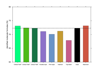
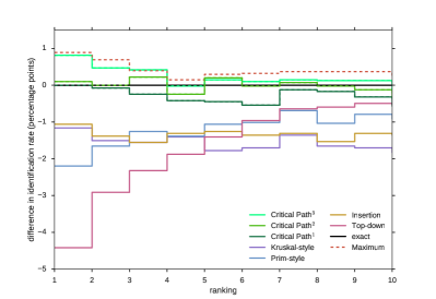
Figure 3: Performance evaluation, finding the correct molecular formula. Left: Percentage of compounds where the correct molecular formula received the highest score. Note the zoom of the y axis. Right: Percentage point difference against exact computations; how often is the correct answer part of the top $k$ output of each method?

First, we evaluated the power of the different heuristics to rank the correct answer (molecular formula) at the top position; see Fig. 3 (left). We also compared against the exact solution. We observe similar identification rates for the critical path heuristics, the maximum heuristic and the exact method. To test whether this trend is true not only for the top rank, but also for the top $k$ ranks, we also evaluated how often any method is capable to rank the correct answer in its top $k$, for varying $k$; see Fig. 3 (right). Identification rates differ much stronger when varying $k$ for one method than for different methods and one $k$; to this end, we normalize identification rates by subtracting the identification rate of the exact method. We see that all heuristics but critical path result in inferior rankings, loosing one or more percentage points for most ranks. In contrast, the critical path heuristics rank solutions with comparable power as the exact method, and the later two variants often outperform the exact method. Somewhat surprisingly, the maximum over all heuristics performs even better than the best heuristic.

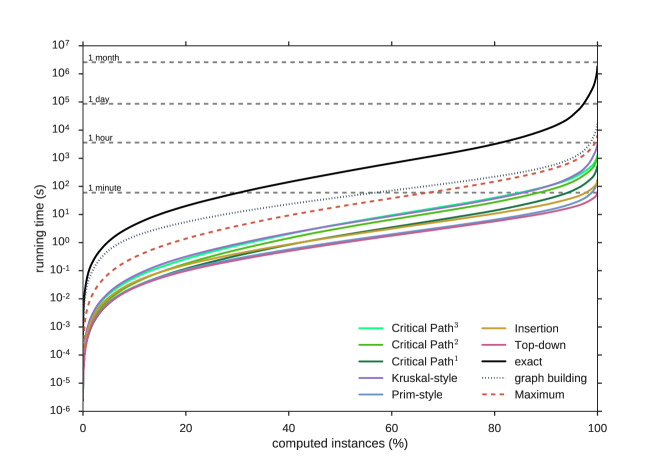
Figure 4: Running times of the different methods. One instances consists of all graphs generated for one compound in the dataset, considering all decompositions of the precursor mass. For each method, instances are sorted with respect to running time, and we report amortized running times. We also report running times for constructing the instance DAGs and for the exact method.

Second, we compared running times of the different methods. Running times were measured using a single thread on an Intel E5-2630v3 at 2.40 GHz with 64 GB RAM. The total running time for the exact methods over all instances is almost one month, underlining the importance of speeding up computations. But also note that solving all instances exactly requires only about 100-fold the time required for constructing the instance graphs. For each method, we sorted all instances by running time; we then reported how much time is required to solve, say, the 90 % “easiest” instances for that method. Generally, this ordering is different for each method. For all methods, we observe that the “hardest” 5 % of the instances are responsible for most of the total running time; this has been observed before [14, 3]. In comparison to the exact method, all heuristics are very fast, and at least two orders of magnitude faster. In particular, each heuristic is faster than the method for constructing the instance graphs; running all heuristics, as required for the maximum heuristic, requires about the same time as the graph construction. Comparing heuristics’ running times, we see that the Kruskal-style heuristic is slowest; and that the first variant of the Critical Path heuristic is faster in practice than variants 2 and 3, but not significantly.

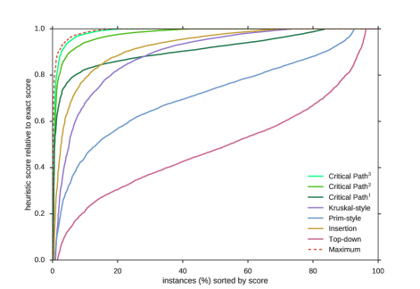
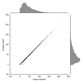
Figure 5: Left: Relative scores of the heuristics. For each Maximum Colorful Subtree instance, we consider the relative score in comparison the exact method at 100 %. For each method, instances are sorted with respect to relative score. Right: Comparison of the score of the Critical Path³ heuristic in comparison to the optimal score of the instance. For each compound, we consider only the true molecular formula candidate.

Third, we compared the scores reached by the different heuristics to the scores of the exact solutions, see Fig. 5 (left). For each compound, we only considered the instance of the Maximum Colorful Subtree that corresponds to the true candidate molecular formula. We report scores relative to the exact solution (at 100 %), and sorted instances with respect to this relative score. In the resulting plot, it is not obvious which of the heuristics “Insertion”, “Kruskal-style” and “Critical Path¹” should be preferred. We see that Critical Path³ heuristic and, hence, the maximum of all methods are able to compute (almost) optimal solutions for about 80 % of the instances. In turn, this means that even for these methods which perform excellent in ranking the correct answer, we miss the optimal solution in about 20 % of the instances. In addition, we compared scores of the Critical Path³ heuristic against the exact method in more detail, see Fig. 5 (right): We see that for instances where the heuristic does not find the optimal solution, the computed solution is only “slightly suboptimal” with respect to its score. In fact, Pearson correlation between the two measures is $+1.00$.

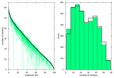
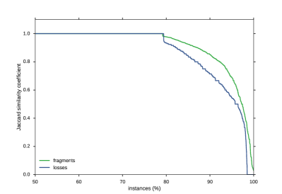
Figure 6: Left: Size of the fragmentation tree. Instances are sorted with respect to the size of the optimal fragmentation tree (black); green bars indicate the corresponding tree sizes for the Critical Path³ heuristic. Middle: Distribution of tree sizes for the exact method (black) and the Critical Path³ heuristic (green). Right: Comparison of the fragmentation tree structure, optimal tree vs. the tree computed by the Critical Path³ heuristic. Note the zoom of the x axis. In all three cases, we consider only the true molecular formula candidate for each compound.

Fourth, we evaluate the solution structure quality of the Critical Path³ heuristic. Unfortunately, the “true fragmentation tree” cannot be determined experimentally [13]. To this end, we compare heuristic tree structure vs. tree structures computed using the exact method. For each compound, we restrict the comparison to the true candidate molecular formula; for other candidate molecular formulas, the optimal tree cannot possibly be the “‘true fragmentation tree”. See Fig. 6. For tree sizes, we observe rather large deviations between heuristic and optimal trees; in contrast, the overall distribution of tree sizes is highly similar. But if we compare tree structures, we observe much larger differences between the Critical Path³ heuristic and the exact method: We measure structural similarity comparing either the set of node labels (fragments) or the set of edge labels (losses) of the two trees. We estimate the similarity of two (finite) sets $A,B$ using the Jaccard similarity coefficient $J(A,B)=\left\lvert A\cap B\right\rvert/\left\lvert A\cup B\right\rvert\in[0,1]$. We observe that more than 20 % of the heuristic trees differ from the corresponding optimal tree; for at least 10 %, this difference is significant.

6 Conclusion

We have presented heuristics for the Maximum Colorful Subtree problem. Our evaluation shows that the Critical Path³ heuristic is well-suited for choosing the correct candidate molecular formula, when applied to tandem mass spectrometry data of small molecules. Our evaluation sidesteps the catch-22 that we want to evaluate solutions based on structure and not score when, at the same time, the correct solution structure is not known. We have shown that the tree computed by the Critical Path³ heuristic is often identical to the optimal tree. Even when the heuristic returns a suboptimal solution, the score is usually very close to the optimal score. In contrast, the structure of the heuristic tree deviates significantly from the optimal tree for more than 20 % of the instances. To this end, we argue not to use this tree for downstream analysis, such as estimating chemical similarity based on fragmentation tree similarity [12] or machine learning [18, 9, 6, 5]: Preliminary evaluations clearly indicate that using trees computed by any heuristic, leads to significantly worse results for the downstream analysis. A back-of-the-envelope calculation indicates the problem: If we assume that 20 % of the heuristic trees are “structurally faulty”, then a pairwise comparison of trees will result in 36 % tree pairs where at least one of the trees is “structurally faulty”.

Building an instance DAG requires more time than running any of the presented heuristics. We conjecture that there is only limited potential for speeding up the graph building phase. To this end, whereas searching for better (and not significantly slower) heuristics is still a valid undertaking, faster heuristics are of little practical use. It is worth mentioning that computing exact solutions for the NP-hard Maximum Colorful Subtree problem takes only about 100-fold the time needed for constructing the graph instances; further speed-up is possible using data reductions and a stronger ILP formulation of the problem from [24].

Even elaborate heuristics for a bioinformatics problem, which are capable of finding solutions with objective function value very close to the optimum, can result in solutions which are structurally very dissimilar from the optimum structure. We showed that this is not only a theoretical possibility, but happens regularly for real-world instances. This underlines the importance of finding exact solutions for bioinformatics problems; the structure of solutions found by heuristic, including local search heuristics such as Markov chain Monte Carlo, may deviate significantly from the optimal solution.

Acknowledgments.

WTJW funded by Deutsche Forschungsgemeinschaft (grant BO 1910/9).

Availability.

The Critical Path³ heuristic and the exact method are available trough the SIRIUS software (https://bio.informatik.uni-jena.de/software/sirius/) and also from GitHub (https://github.com/boecker-lab/sirius). Source code for all other heuristics will be made available upon request. Instances will be made available from our website.

References

- [1] Allen, F., Greiner, R., Wishart, D.: Competitive fragmentation modeling of ESI-MS/MS spectra for putative metabolite identification. Metabolomics 11(1), 98–110 (2015)
- [2] Allen, F., Pon, A., Greiner, R., Wishart, D.: Computational prediction of electron ionization mass spectra to assist in GC/MS compound identification. Anal Chem 88(15), 7689–7697 (2016)
- [3] Böcker, S., Dührkop, K.: Fragmentation trees reloaded. J Cheminform 8, 5 (2016)
- [4] Böcker, S., Rasche, F.: Towards de novo identification of metabolites by analyzing tandem mass spectra. Bioinformatics 24, I49–I55 (2008), proc. of European Conference on Computational Biology (ECCB 2008)
- [5] Brouard, C., Bach, E., Böcker, S., Rousu, J.: Magnitude-preserving ranking for structured outputs. In: Zhang, M.L., Noh, Y.K. (eds.) Proc. of Asian Conference on Machine Learning. Proceedings of Machine Learning Research, vol. 77, pp. 407–422. PMLR (2017)
- [6] Brouard, C., Shen, H., Dührkop, K., d’Alché-Buc, F., Böcker, S., Rousu, J.: Fast metabolite identification with input output kernel regression. Bioinformatics 32(12), i28–i36 (2016), proc. of Intelligent Systems for Molecular Biology (ISMB 2016)
- [7] da Silva, R.R., Dorrestein, P.C., Quinn, R.A.: Illuminating the dark matter in metabolomics. Proc Natl Acad Sci U S A 112(41), 12549–12550 (2015)
- [8] Dondi, R., Fertin, G., Vialette, S.: Complexity issues in vertex-colored graph pattern matching. J Discrete Algorithms 9(1), 82–99 (2011)
- [9] Dührkop, K., Shen, H., Meusel, M., Rousu, J., Böcker, S.: Searching molecular structure databases with tandem mass spectra using CSI:FingerID. Proc Natl Acad Sci U S A 112(41), 12580–12585 (2015)
- [10] Fertin, G., Fradin, J., Jean, G.: Algorithmic aspects of the maximum colorful arborescence problem. In: Proc. of Theory and Applications of Models of Computation (TAMC 2017). Lect Notes Comput Sci, vol. 10185, pp. 216–230 (2017)
- [11] Lacroix, V., Fernandes, C.G., Sagot, M.F.: Motif search in graphs: Application to metabolic networks. IEEE/ACM Trans Comput Biology Bioinform 3(4), 360–368 (2006)
- [12] Rasche, F., Scheubert, K., Hufsky, F., Zichner, T., Kai, M., Svatoš, A., Böcker, S.: Identifying the unknowns by aligning fragmentation trees. Anal Chem 84(7), 3417–3426 (2012)
- [13] Rasche, F., Svatoš, A., Maddula, R.K., Böttcher, C., Böcker, S.: Computing fragmentation trees from tandem mass spectrometry data. Anal Chem 83(4), 1243–1251 (2011)
- [14] Rauf, I., Rasche, F., Nicolas, F., Böcker, S.: Finding maximum colorful subtrees in practice. J Comput Biol 20(4), 1–11 (2013)
- [15] Ridder, L., van der Hooft, J.J.J., Verhoeven, S., de Vos, R.C.H., Bino, R.J., Vervoort, J.: Automatic chemical structure annotation of an LC-MS(n) based metabolic profile from green tea. Anal Chem 85(12), 6033–6040 (2013)
- [16] Ruttkies, C., Schymanski, E.L., Wolf, S., Hollender, J., Neumann, S.: MetFrag relaunched: incorporating strategies beyond in silico fragmentation. J Cheminform 8, 3 (2016)
- [17] Schymanski, E.L., Ruttkies, C., Krauss, M., Brouard, C., Kind, T., Dührkop, K., Allen, F.R., Vaniya, A., Verdegem, D., Böcker, S., Rousu, J., Shen, H., Tsugawa, H., Sajed, T., Fiehn, O., Ghesquière, B., Neumann, S.: Critical Assessment of Small Molecule Identification 2016: Automated methods. J Cheminf 9, 22 (2017)
- [18] Shen, H., Dührkop, K., Böcker, S., Rousu, J.: Metabolite identification through multiple kernel learning on fragmentation trees. Bioinformatics 30(12), i157–i164 (2014), proc. of Intelligent Systems for Molecular Biology (ISMB 2014)
- [19] Stein, S.E.: Mass spectral reference libraries: An ever-expanding resource for chemical identification. Anal Chem 84(17), 7274–7282 (2012)
- [20] Tarjan, R.E.: A class of algorithms which require nonlinear time to maintain disjoint sets. J Comput System Sci 18(2), 110–127 (1979)
- [21] Tsugawa, H., Kind, T., Nakabayashi, R., Yukihira, D., Tanaka, W., Cajka, T., Saito, K., Fiehn, O., Arita, M.: Hydrogen rearrangement rules: Computational ms/ms fragmentation and structure elucidation using MS-FINDER software. Analytical chemistry 88, 7946–7958 (2016)
- [22] Verdegem, D., Lambrechts, D., Carmeliet, P., Ghesquière, B.: Improved metabolite identification with MIDAS and MAGMa through MS/MS spectral dataset-driven parameter optimization. Metabolomics 12(6), 1–16 (2016)
- [23] Wang, M., Carver, J.J., Phelan, V.V., Sanchez, L.M., Garg, N., Peng, Y., Nguyen, D.D., Watrous, J., Kapono, C.A., Luzzatto-Knaan, T., Porto, C., Bouslimani, A., Melnik, A.V., Meehan, M.J., Liu, W.T., Crüsemann, M., Boudreau, P.D., Esquenazi, E., Sandoval-Calderón, M., Kersten, R.D., Pace, L.A., Quinn, R.A., Duncan, K.R., Hsu, C.C., Floros, D.J., Gavilan, R.G., Kleigrewe, K., Northen, T., Dutton, R.J., Parrot, D., Carlson, E.E., Aigle, B., Michelsen, C.F., Jelsbak, L., Sohlenkamp, C., Pevzner, P., Edlund, A., McLean, J., Piel, J., Murphy, B.T., Gerwick, L., Liaw, C.C., Yang, Y.L., Humpf, H.U., Maansson, M., Keyzers, R.A., Sims, A.C., Johnson, A.R., Sidebottom, A.M., Sedio, B.E., Klitgaard, A., Larson, C.B., Boya P, C.A., Torres-Mendoza, D., Gonzalez, D.J., Silva, D.B., Marques, L.M., Demarque, D.P., Pociute, E., O’Neill, E.C., Briand, E., Helfrich, E.J.N., Granatosky, E.A., Glukhov, E., Ryffel, F., Houson, H., Mohimani, H., Kharbush, J.J., Zeng, Y., Vorholt, J.A., Kurita, K.L., Charusanti, P., McPhail, K.L., Nielsen, K.F., Vuong, L., Elfeki, M., Traxler, M.F., Engene, N., Koyama, N., Vining, O.B., Baric, R., Silva, R.R., Mascuch, S.J., Tomasi, S., Jenkins, S., Macherla, V., Hoffman, T., Agarwal, V., Williams, P.G., Dai, J., Neupane, R., Gurr, J., Rodríguez, A.M.C., Lamsa, A., Zhang, C., Dorrestein, K., Duggan, B.M., Almaliti, J., Allard, P.M., Phapale, P., Nothias, L.F., Alexandrov, T., Litaudon, M., Wolfender, J.L., Kyle, J.E., Metz, T.O., Peryea, T., Nguyen, D.T., VanLeer, D., Shinn, P., Jadhav, A., Müller, R., Waters, K.M., Shi, W., Liu, X., Zhang, L., Knight, R., Jensen, P.R., Palsson, B.Ø., Pogliano, K., Linington, R.G., Gutiérrez, M., Lopes, N.P., Gerwick, W.H., Moore, B.S., Dorrestein, P.C., Bandeira, N.: Sharing and community curation of mass spectrometry data with Global Natural Products Social molecular networking. Nat Biotechnol 34(8), 828–837 (2016)
- [24] White, W.T.J., Beyer, S., Dührkop, K., Chimani, M., Böcker, S.: Speedy colorful subtrees. In: Proc. of Computing and Combinatorics Conference (COCOON 2015). Lect Notes Comput Sci, vol. 9198, pp. 310–322. Springer, Berlin (2015)