A Proximal Approach for a Class of Matrix Optimization Problems

Abstract

In recent years, there has been a growing interest in mathematical models leading to the minimization, in a symmetric matrix space, of a Bregman divergence coupled with a regularization term. We address problems of this type within a general framework where the regularization term is split in two parts, one being a spectral function while the other is arbitrary. A Douglas–Rachford approach is proposed to address such problems and a list of proximity operators is provided allowing us to consider various choices for the fit–to–data functional and for the regularization term. Numerical experiments show the validity of this approach for solving convex optimization problems encountered in the context of sparse covariance matrix estimation. Based on our theoretical results, an algorithm is also proposed for noisy graphical lasso where a precision matrix has to be estimated in the presence of noise. The nonconvexity of the resulting objective function is dealt with a majorization–minimization approach, i.e. by building a sequence of convex surrogates and solving the inner optimization subproblems via the aforementioned Douglas–Rachford procedure. We establish conditions for the convergence of this iterative scheme and we illustrate its good numerical performance with respect to state–of–the–art approaches.

1 Introduction

In recent years, various applications such as shape classification models DBLP:conf/uai/2008 , gene expression Ma:2013:ADM:2494250.2494257 , model selection Banerjee:2008:MST:1390681.1390696 ; chandrasekaran2012 , computer vision doi:10.1093/biomet/asq060 , inverse covariance estimation Friedman07 ; Dempster72 ; Yuan09 ; Aspremont08 ; doi:10.1137/090772514 , graph estimation meinshausen2006 ; ravikumar2011 ; doi:10.1093/biomet/asm018 , social network and corporate inter-relationships analysis Aslan2016 , or brain network analysis doi:10.1137/130936397 have led to matrix variational formulations of the form:

$$\underset{\begin{subarray}{c}{\mathbf{C}\in\mathcal{S}_{n}}\end{subarray}}{\operatorname{minimize}}\,\,{f(\mathbf{C})-\operatorname{trace}\left({\mathbf{T}\mathbf{C}}\right)+g(\mathbf{C})},$$ (1)

where $\mathcal{S}_{n}$ is the set of real symmetric matrices of dimension $n\times n$, $\mathbf{T}$ is a given $n\times n$ real matrix (without loss of generality, it will be assumed to be symmetric), and $f\colon\mathcal{S}_{n}\to]-\infty,+\infty]$ and $g\colon\colon\mathcal{S}_{n}\to]-\infty,+\infty]$ are lower-semicontinuous functions which are proper, in the sense that they are finite at least in one point.
It is worth noticing that the notion of Bregman divergence bregman1967 gives a particular insight into Problem (1). Indeed, suppose that $f$ is a convex function differentiable on the interior of its domain $\operatorname{int}(\operatorname{dom}f)\neq\varnothing$. Let us recall that, in $\mathcal{S}_{n}$ endowed with the Frobenius norm, the $f$-Bregman divergence between $\mathbf{C}\in\mathcal{S}_{n}$ and $\mathbf{Y}\in\operatorname{int}(\operatorname{dom}f)$ is

$$D^{f}(\mathbf{C},\mathbf{Y})=f(\mathbf{C})-f(\mathbf{Y})-\operatorname{trace}\left({\mathbf{T}(\mathbf{C}-\mathbf{Y})}\right),$$ (2)

where $\mathbf{T}=\nabla f(\mathbf{Y})$ is the gradient of $f$ at $\mathbf{Y}$. Hence, the original problem (1) is equivalently expressed as

$$\underset{\begin{subarray}{c}{\mathbf{C}\in\mathcal{S}_{n}}\end{subarray}}{\operatorname{minimize}}\,\,g(\mathbf{C})+D^{f}(\mathbf{C},\mathbf{Y}).$$ (3)

Solving Problem (3) amounts to computing the proximity operator of $g$ at $\mathbf{Y}$ with respect to the divergence $D^{f}$ Bauschke03 ; Bauschke06 in the space $\mathcal{S}_{n}$. In the vector case, such kind of proximity operator has been found to be useful in a number of recent works regarding, for example, image restoration Brune2011 ; Benfenati13 ; Benfenati2015 ; doi:10.1137/090746379 , image reconstruction Zhang2011 , and compressive sensing problems Yin08 ; doi:10.1137/080725891 .
In this paper, it will be assumed that $f$ belongs to the class of spectral functions (borwein2014, , Chapter 5, Section 2), i.e., for every permutation matrix $\mathbf{\Sigma}\in\mathbb{R}^{n\times n}$,

$$(\forall\mathbf{C}\in\mathcal{S}_{n})\quad f(\mathbf{C})=\varphi(\mathbf{\Sigma}\mathbf{d}),$$ (4)

where $\varphi\colon\mathbb{R}^{n}\to]-\infty,+\infty]$ is a proper lower semi-continuous convex function and $\mathbf{d}$ is a vector of eigenvalues of $\mathbf{C}$.
Due to the nature of the problems, in many of the aforementioned applications, $g$ is a regularization function promoting the sparsity of $\mathbf{C}$. We consider here a more generic class of regularization functions obtained by decomposing $g$ as $g_{0}+g_{1}$, where $g_{0}$ is a spectral function, i.e., for every permutation matrix $\mathbf{\Sigma}\in\mathbb{R}^{n\times n}$,

$$(\forall\mathbf{C}\in\mathcal{S}_{n})\quad g_{0}(\mathbf{C})=\psi(\mathbf{\Sigma}\mathbf{d}),$$ (5)

with $\psi\colon\mathbb{R}^{n}\to]-\infty,+\infty]$ a proper lower semi–continuous function, $\mathbf{d}$ still denoting a vector of the eigenvalues of $\mathbf{C}$, while $g_{1}\colon\mathcal{S}_{n}\to]-\infty,+\infty]$ is a proper lower semi–continuous function which cannot be expressed under a spectral form. A very popular and useful example encompassed by our framework is the graphical lasso (GLASSO) problem, where $f$ is the minus log-determinant function, $g_{1}$ is a component–wise $\ell_{1}$ norm (of the matrix elements), and $g_{0}\equiv 0$. Various algorithms have been proposed to solve Problem (1) in this context, including the popular GLASSO algorithm Friedman07 and some of its recent variants mazumder2012 . We can also mention the dual block coordinate ascent method from Banerjee:2008:MST:1390681.1390696 , the SPICE algorithm rothman2008 , the gradient projection method in DBLP:conf/uai/2008 , the Refitted CLIME algorithm doi:10.1198/jasa.2011.tm10155 , various algorithms Aspremont08 ; doi:10.1137/070695915 ; doi:10.1137/080742531 based on Nesterov’s smooth gradient approach Nesterov2005 , ADMM approaches Yuan09 ; NIPS2010_0109 , an inexact Newton method doi:10.1137/090772514 , and interior point methods doi:10.1093/biomet/asm018 ; Li2010 . A related model is addressed in Ma:2013:ADM:2494250.2494257 ; chandrasekaran2012 , with the additional assumption that the sought solution can be split as $\mathbf{C}_{1}+\mathbf{C}_{2}$, where $\mathbf{C}_{1}$ is sparse and $\mathbf{C}_{2}$ is low–rank. Finally, let us mention the ADMM algorithm from Zhou14 , and the incremental proximal gradient approach from Richard:2012:ESS:3042573.3042584 , both addressing Problem (1) when $f$ is the squared Frobenius norm, $g_{0}$ is a nuclear norm, and $g_{1}$ is an element–wise $\ell_{1}$ norm.

The main goal of this paper is to propose numerical approaches for solving Problem (1). Two settings will be investigated, namely (i) $g_{1}\equiv 0$, i.e. the whole cost function is a spectral one, (ii) $g_{1}\not\equiv 0$. In the former case, some general results concerning the $D^{f}$-proximity operator of $g_{0}$ are established. In the latter case, a Douglas–Rachford optimization method is proposed, which leads us to calculate the proximity operators of several spectral functions of interest. We then consider applications of our results to the estimation of (possibly low-rank) covariance matrices from noisy observations of multivalued random variables. Two variational approaches are proposed for estimating the unknown covariance matrix, depending on the prior assumptions made on it. We show that the cost function arising from the first formulation can be minimized through our proposed Douglas-Rachford procedure under mild assumptions on the involved regularization functions. The second formulation of the problem aims at preserving desirable sparsity properties of the inverse covariance (i.e., precision) matrix. We establish that the proposed objective function is a difference of convex terms, and we introduce a novel majorization-minimization (MM) algorithm to optimize it.

The paper is organized as follows. Section 2 is devoted to the solution of the particular instance of Problem (1) corresponding to $g_{1}\equiv 0$. Section 3 describes a proximal minimization algorithm to address the problem when $g_{1}\not\equiv 0$. Its implementation is discussed for a bunch of useful choices for the involved functionals. Section 4 presents two new approaches for estimating covariance matrices from noisy data. Finally, in Section 5, numerical experiments illustrate the applicability of the proposed methods, and its good performance with respect to the state-of-the-art, in two distinct scenarios.

Notation: Greek letters usually designate real numbers, bold letters designate vectors in a Euclidean space, capital bold letters indicate matrices. The $i$–th element of the vector $\mathbf{d}$ is denoted by $d_{i}$. $\operatorname{Diag}(\mathbf{d})$ denotes the diagonal matrix whose diagonal elements are the components of $\mathbf{d}$. $\mathcal{D}_{n}$ is the cone of vectors $\mathbf{d}\in\mathbb{R}^{n}$ whose components are ordered by decreasing values. The symbol $\operatorname{vect}(\mathbf{C})$ denotes the vector resulting from a column–wise ordering of the elements of matrix $\mathbf{C}$. The product $\mathbf{A}\otimes\mathbf{B}$ denotes the classical Kronecker product of matrices $\mathbf{A}$ and $\mathbf{B}$. Let $\mathcal{H}$ be a real Hilbert space endowed with an inner product $\langle\cdot,\cdot\rangle$ and a norm $\|\cdot\|$, the domain of a function $f\colon\mathcal{H}\to]-\infty,+\infty]$ is $\operatorname{dom}f=\{x\in\mathcal{H}\mid f(x)<+\infty\}$. $f$ is coercive if $\lim_{\|x\|\to+\infty}f(x)=+\infty$ and supercoercive if $\lim_{\|x\|\to+\infty}f(x)/\|x\|=+\infty$. The Moreau subdifferential of $f$ at $x\in\mathcal{H}$ is $\partial f(x)=\{t\in\mathcal{H}\mid(\forall y\in\mathcal{H})f(y)\geq f(x)+\langle t,y-x\rangle\}$. $\Gamma_{0}(\mathcal{H})$ denotes the class of lower-semicontinuous convex functions from $\mathcal{H}$ to $]-\infty,+\infty]$ with a nonempty domain (proper). If $f\in\Gamma_{0}(\mathcal{H})$ is (Gâteaux) differentiable at $x\in\mathcal{H}$, then $\partial f(x)=\{\nabla f(x)\}$ where $\nabla f(x)$ is the gradient of $f$ at $x$. If a function $f\colon\mathcal{H}\to]-\infty,+\infty]$ possesses a unique minimizer on a set $E\subset\mathcal{H}$, it will be denoted by $\underset{\begin{subarray}{c}{x\in E}\end{subarray}}{\operatorname{argmin}}\,\,{f(x)}$. If there are possibly several minimizers, their set will be denoted by $\underset{\begin{subarray}{c}{x\in E}\end{subarray}}{\operatorname{Argmin}}\,\,{f(x)}$. Given a set $E$, $\operatorname{int}(E)$ designates the interior of $E$ and $\iota_{E}$ denotes the indicator function of the set, which is equal to $0$ over this set and $+\infty$ otherwise. In the remainder of the paper, the underlying Hilbert space will be $\mathcal{S}_{n}$, the set of real symmetric matrices equipped with the Frobenius norm, denoted by $\|\cdot\|_{\rm F}$. The matrix spectral norm is denoted by $\|\cdot\|_{\rm S}$, the $\ell_{1}$ norm of a matrix $\mathbf{A}=(A_{i,j})_{i,j}$ is $\|\mathbf{A}\|_{1}=\sum_{i,j}|A_{i,j}|$. For every $p\in[1,+\infty[$, $\mathcal{R}_{p}\left({\cdot}\right)$ denotes the Schatten $p$–norm, the nuclear norm being obtained when $p=1$. $\mathcal{O}_{n}$ denotes the set of orthogonal matrices of dimension $n$ with real elements; $\mathcal{S}_{n}^{+}$ and $\mathcal{S}_{n}^{++}$ denote the set of real symmetric positive semidefinite, and symmetric positive definite matrices, respectively, of dimension $n$. $\textnormal{I}_{\textnormal{d}}$ denotes the identity matrix whose dimension will be clear from the context. The soft thresholding operator $\operatorname{soft}_{\mu}$ and the hard thresholding operator $\operatorname{hard}_{\mu}$ of parameter $\mu\in[0,+\infty[$ are given by

$$(\forall\xi\in\mathbb{R})\qquad\operatorname{soft}_{\mu}(\xi)=\begin{cases}\xi-\mu&\mbox{if $\xi>\mu$}\\ \xi+\mu&\mbox{if $\xi<-\mu$}\\ 0&\mbox{otherwise}\end{cases},\qquad\operatorname{hard}_{\mu}(\xi)=\begin{cases}\xi&\mbox{if $|\xi|>\mu$}\\ 0&\mbox{otherwise.}\end{cases}$$ (6)

2 Spectral Approach

In this section, we show that, in the particular case when $g_{1}\equiv 0$, Problem (1) reduces to the optimization of a function defined on $\mathbb{R}^{n}$. Indeed, the problem then reads:

$$\underset{\begin{subarray}{c}{\mathbf{C}\in\mathcal{S}_{n}}\end{subarray}}{\operatorname{minimize}}\,\,{f(\mathbf{C})-\operatorname{trace}\left({\mathbf{T}\mathbf{C}}\right)+g_{0}(\mathbf{C})},$$ (7)

where the spectral forms of $f$ and $g_{0}$ allow us to take advantage of the eigendecompositions of $\mathbf{C}$ and $\mathbf{T}$ in order to simplify the optimization problem, as stated below.

Theorem 2.1

Let $\mathbf{t}\in\mathbb{R}^{n}$ be a vector of eigenvalues of $\mathbf{T}$ and let $\mathbf{U}_{\mathbf{T}}\in\mathcal{O}_{n}$ be such that $\mathbf{T}=\mathbf{U}_{T}\operatorname{Diag}(\mathbf{t})\mathbf{U}_{T}^{\top}$. Let $f$ and $g_{0}$ be functions satisfying (4) and (5), respectively, where $\varphi$ and $\psi$ are lower-semicontinuous functions. Assume that $\operatorname{dom}\varphi\cap\operatorname{dom}\psi\neq\varnothing$ and that the function $\mathbf{d}\mapsto\varphi(\mathbf{d})-\mathbf{d}^{\top}\mathbf{t}+\psi(\mathbf{d})$ is coercive. Then a solution to Problem (7) exists, which is given by

$$\widehat{\mathbf{C}}=\mathbf{U}_{\mathbf{T}}\operatorname{Diag}(\widehat{\mathbf{d}})\mathbf{U}_{\mathbf{T}}^{\top}$$ (8)

where $\widehat{\mathbf{d}}$ is any solution to the following problem:

$$\underset{\begin{subarray}{c}{\mathbf{d}\in\mathbb{R}^{n}}\end{subarray}}{\operatorname{minimize}}\,\,\varphi(\mathbf{d})-\mathbf{d}^{\top}\mathbf{t}+\psi(\mathbf{d}).$$ (9)

For the sake of clarity, before establishing this result, we recall two useful lemmas from linear algebra.

Lemma 1

(marshall11, , Chapter 9, Sec. H, p. 340) Let $\mathbf{C}\in\mathcal{S}_{n}$ and let $\mathbf{d}\in\mathcal{D}_{n}$ be a vector of ordered eigenvalues of this matrix. Let $\mathbf{T}\in\mathcal{S}_{n}$ and let $\mathbf{t}\in\mathcal{D}_{n}$ be a vector of ordered eigenvalues of this matrix. The following inequality holds:

$$\operatorname{trace}\left({\mathbf{C}\mathbf{T}}\right)\leq\mathbf{d}^{\top}\mathbf{t}.$$ (10)

In addition, the upper bound is reached if and only if $\mathbf{T}$ and $\mathbf{C}$ share the same eigenbasis, i.e. there exists $\mathbf{U}\in\mathcal{O}_{n}$ such that $\mathbf{C}=\mathbf{U}\operatorname{Diag}(\mathbf{d})\mathbf{U}^{\top}$ and $\mathbf{T}=\mathbf{U}\operatorname{Diag}(\mathbf{t})\mathbf{U}^{\top}$.

The subsequent lemma is also known as the rearrangement inequality:

Lemma 2

(hardy1952inequalities, , Section 10.2, Theorem 368) Let $\mathbf{a}\in\mathcal{D}_{n}$ and $\mathbf{b}\in\mathcal{D}_{n}$. Then, for every permutation matrix $\mathbf{P}$ of dimension $n\times n$,

$$\mathbf{a}^{\top}\mathbf{P}\mathbf{b}\leq\mathbf{a}^{\top}\mathbf{b}.$$ (11)

We are now ready to prove Theorem 2.1.

Proof (Theorem 2.1)

Due to the assumptions made on $f$ and $g_{0}$, Problem (7) can be reformulated as

$$\underset{\begin{subarray}{c}{\mathbf{d}\in\mathcal{D}_{n},\mathbf{U}_{\mathbf{C}}\in\mathcal{O}_{n}}\end{subarray}}{\operatorname{minimize}}\,\,\varphi(\mathbf{d})-\operatorname{trace}\left({\mathbf{U}_{\mathbf{C}}\operatorname{Diag}(\mathbf{d})\mathbf{U}_{\mathbf{C}}^{\top}\mathbf{T}}\right)+\psi(\mathbf{d}).$$

According to the first claim in 1,

$$\inf_{\mathbf{d}\in\mathcal{D}_{n},\mathbf{U}_{\mathbf{C}}\in\mathcal{O}_{n}}\varphi(\mathbf{d})-\operatorname{trace}\left({\mathbf{U}_{\mathbf{C}}\operatorname{Diag}(\mathbf{d})\mathbf{U}_{\mathbf{C}}^{\top}\mathbf{T}}\right)+\psi(\mathbf{d})\geq\inf_{\mathbf{d}\in\mathcal{D}_{n}}\varphi(\mathbf{d})-\mathbf{d}^{\top}\widetilde{\mathbf{t}}+\psi(\mathbf{d}),$$

where $\widetilde{\mathbf{t}}\in\mathcal{D}_{n}$ is the vector of ordered eigenvalues of $\mathbf{T}=\widetilde{\mathbf{U}}_{\mathbf{T}}\operatorname{Diag}(\widetilde{\mathbf{t}})\widetilde{\mathbf{U}}_{\mathbf{T}}^{\top}$ with $\widetilde{\mathbf{U}}_{\mathbf{T}}\in\mathcal{O}_{n}$. In addition, the last claim in 1 allows us to conclude that the lower bound is attained when $\mathbf{U}_{\mathbf{C}}=\widetilde{\mathbf{U}}_{\mathbf{T}}$. This proves that

$$\inf_{\mathbf{C}\in\mathcal{S}_{n}}{f(\mathbf{C})-\operatorname{trace}\left({\mathbf{T}\mathbf{C}}\right)+g_{0}(\mathbf{C})}=\inf_{\mathbf{d}\in\mathcal{D}_{n}}\varphi(\mathbf{d})-\mathbf{d}^{\top}\widetilde{\mathbf{t}}+\psi(\mathbf{d}).$$ (12)

Let us now show that ordering the eigenvalues is unnecessary for our purposes. Let $\mathbf{t}\in\mathbb{R}^{n}$ be a vector of non necessarily ordered eigenvalues of $\mathbf{T}$. Then, $\mathbf{T}=\mathbf{U}_{\mathbf{T}}\operatorname{Diag}(\mathbf{t})\mathbf{U}_{\mathbf{T}}^{\top}$ with $\mathbf{U}_{\mathbf{T}}\in\mathcal{O}_{n}$ and there exists a permutation matrix $\mathbf{Q}$ such that $\mathbf{t}=\mathbf{Q}\widetilde{\mathbf{t}}$. For every vector $\mathbf{d}\in\mathcal{D}_{n}$ and for every permutation matrix $\mathbf{P}$ of dimension $n\times n$, we have then

$$\varphi(\mathbf{P}\mathbf{d})-(\mathbf{P}\mathbf{d})^{\top}\mathbf{t}+\psi(\mathbf{P}\mathbf{d})= \,\varphi(\mathbf{P}\mathbf{d})-(\mathbf{P}\mathbf{d})^{\top}\mathbf{Q}\widetilde{\mathbf{t}}+\psi(\mathbf{P}\mathbf{d})$$ (13)

$$= \,\varphi(\mathbf{d})-(\mathbf{Q}^{\top}\mathbf{P}\mathbf{d})^{\top}\widetilde{\mathbf{t}}+\psi(\mathbf{d})$$

$$\geq \,\varphi(\mathbf{d})-\mathbf{d}^{\top}\widetilde{\mathbf{t}}+\psi(\mathbf{d}),$$

where the last inequality is a direct consequence of 2. In addition, the equality is obviously reached if $\mathbf{P}=\mathbf{Q}$. Since every vector in $\mathbb{R}^{n}$ can be expressed as permutation of a vector in $\mathcal{D}_{n}$, we deduce that

$$\inf_{\mathbf{d}\in\mathbb{R}^{n}}\varphi(\mathbf{d})-\mathbf{d}^{\top}\mathbf{t}+\psi(\mathbf{d})=\inf_{\mathbf{d}\in\mathcal{D}_{n}}\varphi(\mathbf{d})-\mathbf{d}^{\top}\widetilde{\mathbf{t}}+\psi(\mathbf{d}).$$ (14)

Altogether, (12) and (14) lead to

$$\inf_{\mathbf{C}\in\mathcal{S}_{n}}{f(\mathbf{C})-\operatorname{trace}\left({\mathbf{T}\mathbf{C}}\right)+g_{0}(\mathbf{C})}=\inf_{\mathbf{d}\in\mathbb{R}^{n}}\varphi(\mathbf{d})-\mathbf{d}^{\top}\mathbf{t}+\psi(\mathbf{d}).$$ (15)

Since the function $\mathbf{d}\mapsto\varphi(\mathbf{d})-\mathbf{d}^{\top}\mathbf{t}+\psi(\mathbf{d})$ is proper, lower-semicontinuous, and coercive, it follows from (Rockfellar97, , Theorem 1.9) that there exists $\widehat{\mathbf{d}}\in\mathbb{R}^{n}$ such that

$$\varphi(\widehat{\mathbf{d}})-\widehat{\mathbf{d}}^{\top}\mathbf{t}+\psi(\widehat{\mathbf{d}})=\inf_{\mathbf{d}\in\mathbb{R}^{n}}\varphi(\mathbf{d})-\mathbf{d}^{\top}\mathbf{t}+\psi(\mathbf{d}).$$ (16)

In addition, it is easy to check that if $\widehat{\mathbf{C}}$ is given by (8) then

$$f(\widehat{\mathbf{C}})-\operatorname{trace}\left({\mathbf{T}\widehat{\mathbf{C}}}\right)+g_{0}(\widehat{\mathbf{C}})=\varphi(\widehat{\mathbf{d}})-\widehat{\mathbf{d}}^{\top}\mathbf{t}+\psi(\widehat{\mathbf{d}}),$$ (17)

which yields the desired result.∎

Before deriving a main consequence of this result, we need to recall some definitions from convex analysis (Rockfellar70, , Chapter 26) (Bauschke03, , Section 3.4):

Definition 1

Let $\mathcal{H}$ be a finite dimensional real Hilbert space with norm $\|\cdot\|$ and scalar product $\langle\cdot,\cdot\rangle$. Let $h\colon\mathcal{H}\to]-\infty,+\infty]$ be a proper convex function.

• $h$ is essentially smooth if $h$ is differentiable on $\operatorname{int}(\operatorname{dom}h)\neq\varnothing$ and$\lim_{n\to+\infty}\|\nabla h(x_{n})\|=+\infty$ for every sequence $(x_{n})_{n\in\mathbb{N}}$ of $\operatorname{int}(\operatorname{dom}h)$ converging to a point on the boundary of $\operatorname{dom}h$.

• $h$ is essentially strictly convex if $h$ is strictly convex on every convex subset of the domain of its subdifferential.

• $h$ is a Legendre function if it is both essentially smooth and essentially strictly convex.

• If $h$ is differentiable on $\operatorname{int}(\operatorname{dom}h)\neq\varnothing$, the $h$-Bregman divergence is the function $D^{h}$ defined on $\mathcal{H}^{2}$ as

  $$(\forall(x,y)\in\mathcal{H}^{2})\\ D^{h}(x,y)=\begin{cases}h(x)-h(y)-\langle\nabla h(y),x-y\rangle&\mbox{if $y\in\operatorname{int}(\operatorname{dom}f)$}\\ +\infty&\mbox{otherwise.}\end{cases}$$ (18)

• Assume that $h$ is a lower-semicontinuous Legendre function and that $\ell$ is a lower-semicontinuous convex function such that $\operatorname{int}(\operatorname{dom}h)\cap\operatorname{dom}\ell\neq\varnothing$ and either $\ell$ is bounded from below or $h+\ell$ is supercoercive. Then, the $D^{h}$-proximity operator of $\ell$ is

  $$\operatorname{prox}^{h}_{\ell}\colon\operatorname{int}(\operatorname{dom}h) \to\operatorname{int}(\operatorname{dom}h)\cap\operatorname{dom}\ell$$ (19)

  $$y \mapsto\underset{\begin{subarray}{c}{x\in\mathcal{H}}\end{subarray}}{\operatorname{argmin}}\,\,{\ell(x)+D^{h}(x,y)}.$$

In this definition, when $h=\|\cdot\|^{2}/2$, we recover the classical definition of the proximity operator in Moreau65 , which is defined over $\mathcal{H}$, for every function $\ell\in\Gamma_{0}(\mathcal{H})$, and that will be simply denoted by $\operatorname{prox}_{\ell}$.

We will also need the following result:

Lemma 3

Let $f$ be a function satisfying (4) where $\varphi\colon\mathbb{R}^{n}\to]-\infty,+\infty]$. Let $\mathbf{C}\in\mathcal{S}_{n}$ and let $\mathbf{d}\in\mathbb{R}^{n}$ be a vector of eigenvalues of this matrix. The following hold:

1. $\mathbf{C}\in\operatorname{dom}f$ if and only if $\mathbf{d}\in\operatorname{dom}\varphi$;

2. $\mathbf{C}\in\operatorname{int}(\operatorname{dom}f)$ if and only if $\mathbf{d}\in\operatorname{int}(\operatorname{dom}\varphi)$.

Proof

(i) obviously holds since $f$ is a spectral function.
Let us now prove (ii). If $\mathbf{C}\in\operatorname{int}(\operatorname{dom}f)$, then $\mathbf{d}\in\operatorname{dom}\varphi$. In addition, there exists $\rho\in]0,+\infty[$ such that, for every $\mathbf{C}^{\prime}\in\mathcal{S}_{n}$, if $\|\mathbf{C}^{\prime}-\mathbf{C}\|_{\rm F}\leq\rho$, then $\mathbf{C}^{\prime}\in\operatorname{dom}f$. Let $\mathbf{U}_{\mathbf{C}}\in\mathcal{O}_{n}$ be such that $\mathbf{C}=\mathbf{U}_{\mathbf{C}}\operatorname{Diag}(\mathbf{d})\mathbf{U}_{\mathbf{C}}^{\top}$ and let us choose $\mathbf{C}^{\prime}=\mathbf{U}_{\mathbf{C}}\operatorname{Diag}(\mathbf{d}^{\prime})\mathbf{U}_{\mathbf{C}}^{\top}$ with $\mathbf{d}^{\prime}\in\mathbb{R}^{n}$. Since $\mathbf{C}$ and $\mathbf{C}^{\prime}$ share the same eigenbasis,

$$\|\mathbf{C}^{\prime}-\mathbf{C}\|_{\rm F}=\|\mathbf{d}^{\prime}-\mathbf{d}\|.$$ (20)

Hence, for any $\mathbf{d}^{\prime}\in\mathbb{R}^{n}$ such that $\|\mathbf{d}^{\prime}-\mathbf{d}\|\leq\rho$, $\mathbf{C}^{\prime}\in\operatorname{dom}f$, hence $\mathbf{d}^{\prime}\in\operatorname{dom}\varphi$. This shows that $\mathbf{d}\in\operatorname{int}(\operatorname{dom}\varphi)$.
Conversely, let us assume that $\mathbf{d}=(d_{i})_{1\leq i\leq n}\in\operatorname{int}(\operatorname{dom}\varphi)$. Without loss of generality, it can be assumed that $\mathbf{d}\in\mathcal{D}_{n}$. There thus exists $\rho\in]0,+\infty[$ such that for every $\mathbf{d}^{\prime}=(d^{\prime}_{i})_{1\leq i\leq n}\in\mathcal{D}_{n}$, if

$$(\forall i\in\{1,\ldots,n\})\qquad|d^{\prime}_{i}-d_{i}|\leq\rho,$$ (21)

then $\mathbf{d}^{\prime}\in\operatorname{dom}\varphi$. Furthermore, let $\mathbf{C}^{\prime}$ be any matrix in $\mathcal{S}_{n}$ such that

$$\|\mathbf{C}^{\prime}-\mathbf{C}\|_{\rm F}\leq\rho$$ (22)

and let $\mathbf{d}^{\prime}=(d^{\prime}_{i})_{1\leq i\leq n}\in\mathcal{D}_{n}$ be a vector of eigenvalues of $\mathbf{C}$. It follows from Weyl’s inequality marshall11 that

$$(\forall i\in\{1,\ldots,n\})\qquad|d^{\prime}_{i}-d_{i}|\leq\|\mathbf{C}^{\prime}-\mathbf{C}\|_{\rm S}\leq\|\mathbf{C}^{\prime}-\mathbf{C}\|_{\rm F}\leq\rho.$$ (23)

We deduce that $\mathbf{d}^{\prime}\in\operatorname{dom}\varphi$ and, consequently $\mathbf{C}^{\prime}\in\operatorname{dom}f$. This shows that $\mathbf{C}\in\operatorname{int}(\operatorname{dom}f)$. ∎

As an offspring of Theorem 2.1, we then get:

Corollary 1

Let $f$ and $g_{0}$ be functions satisfying (4) and (5), respectively, where $\varphi\in\Gamma_{0}(\mathbb{R}^{n})$ is a Legendre function, $\psi\in\Gamma_{0}(\mathbb{R}^{n})$, $\operatorname{int}(\operatorname{dom}\varphi)\cap\operatorname{dom}\psi\neq\varnothing$, and either $\psi$ is bounded from below or $\varphi+\psi$ is supercoercive. Then, the $D^{f}$-proximity operator of $g_{0}$ is defined at every $\mathbf{Y}\in\mathcal{S}_{n}$ such that $\mathbf{Y}=\mathbf{U}_{\mathbf{Y}}\operatorname{Diag}(\mathbf{y})\mathbf{U}_{\mathbf{Y}}^{\top}$ with $\mathbf{U}_{\mathbf{Y}}\in\mathcal{O}_{n}$ and $\mathbf{y}\in\operatorname{int}(\operatorname{dom}\varphi)$, and it is expressed as

$$\operatorname{prox}^{f}_{g_{0}}(\mathbf{Y})=\mathbf{U}_{\mathbf{Y}}\operatorname{Diag}(\operatorname{prox}^{\varphi}_{\psi}(\mathbf{y}))\mathbf{U}_{\mathbf{Y}}^{\top}.$$ (24)

Proof

According to the properties of spectral functions (Lewis96, , Corollary 2.7),

$$\varphi\in\Gamma_{0}(\mathbb{R}^{n})\;\mbox{(resp. $\psi\in\Gamma_{0}(\mathbb{R}^{n})$)}\quad\Rightarrow\quad f\in\Gamma_{0}(\mathcal{S}_{n})\>\mbox{(resp. $g_{0}\in\Gamma_{0}(\mathcal{S}_{n})$)}.$$ (25)

In addition, according to (Lewis96, , Corollaries 3.3&3.5), since $\varphi$ is a Legendre function, $f$ is a Legendre function. It is also straightforward to check that, when $\psi$ is lower bounded, then $g_{0}$ is lower bounded and, when $\varphi+\psi$ is supercoercive, then $f+g_{0}$ is supercoercive. It also follows from 3 that $\operatorname{int}(\operatorname{dom}\varphi)\cap\operatorname{dom}\psi\neq\varnothing\Leftrightarrow\operatorname{int}(\operatorname{dom}f)\cap\operatorname{dom}g_{0}\neq\varnothing$.

The above results show that the $D^{f}$-proximity operator of $g_{0}$ is properly defined as follows:

$$\operatorname{prox}^{f}_{g_{0}}\colon\operatorname{int}(\operatorname{dom}f) \to\operatorname{int}(\operatorname{dom}f)\cap\operatorname{dom}g_{0}$$ (26)

$$\mathbf{Y} \mapsto\underset{\begin{subarray}{c}{\mathbf{C}\in\mathcal{S}_{n}}\end{subarray}}{\operatorname{argmin}}\,\,{g_{0}(\mathbf{C})+D^{f}(\mathbf{C},\mathbf{Y})}.$$

This implies that computing the $D^{f}$-proximity operator of $g_{0}$ at $\mathbf{Y}\in\operatorname{int}(\operatorname{dom}f)$ amounts to finding the unique solution to Problem (7) where $\mathbf{T}=\nabla f(\mathbf{Y})$. Let $\mathbf{Y}=\mathbf{U}_{\mathbf{Y}}\operatorname{Diag}(\mathbf{y})\mathbf{U}_{\mathbf{Y}}^{\top}$ with $\mathbf{U}_{\mathbf{Y}}\in\mathcal{O}_{n}$ and $\mathbf{y}\in\mathbb{R}^{n}$. By 3(ii), $\mathbf{Y}\in\operatorname{int}(\operatorname{dom}f)\Leftrightarrow\mathbf{y}\in\operatorname{int}(\operatorname{dom}(\varphi))$ and, according to (Lewis96, , Corollary 3.3), $\mathbf{T}=\mathbf{U}_{\mathbf{Y}}\operatorname{Diag}(\mathbf{t})\mathbf{U}_{\mathbf{Y}}^{\top}$ with $\mathbf{t}=\nabla\varphi(\mathbf{y})$.

Furthermore, as $\varphi$ is essentially strictly convex, it follows from (Bauscke-Borwein01, , Theorem 5.9(ii)) that $\mathbf{t}=\nabla\varphi(\mathbf{y})\in\operatorname{int}(\operatorname{dom}f^{*})$, which according to (Bauschke:2017, , Theorem 14.17) is equivalent to the fact that $\mathbf{d}\mapsto\varphi(\mathbf{d})-\mathbf{d}^{\top}\mathbf{t}$ is coercive. So, if $\psi$ is lower-bounded, $\mathbf{d}\mapsto\varphi(\mathbf{d})-\mathbf{d}^{\top}\mathbf{t}+\psi(\mathbf{d})$ is coercive. The same conclusion obviously holds if $\varphi+\psi$ is supercoercive. This shows that the assumptions of Theorem 2.1 are met. Consequently, applying this theorem yields

$$\operatorname{prox}^{f}_{g_{0}}(\mathbf{Y})=\mathbf{U}_{\mathbf{Y}}\operatorname{Diag}(\widehat{\mathbf{d}})\mathbf{U}_{\mathbf{Y}}^{\top},$$ (27)

where $\widehat{\mathbf{d}}$ minimizes

$$\mathbf{d}\mapsto\varphi(\mathbf{d})-\mathbf{d}^{\top}\mathbf{t}+\psi(\mathbf{d})$$ (28)

or, equivalently,

$$\mathbf{d}\mapsto\psi(\mathbf{d})+D^{\varphi}(\mathbf{d},\mathbf{y}).$$ (29)

This shows that $\widehat{\mathbf{d}}=\operatorname{prox}^{\varphi}_{\psi}(\mathbf{y})$.∎

Remark 1

1 extends known results concerning the case when $f=$$\|\cdot\|_{\rm F}/2$ Cai10 . A rigorous derivation of the proximity operator of spectral functions in $\Gamma_{0}(\mathcal{S}_{n})$ for the standard Frobenius metric can be found in (Bauschke:2017, , Corollary 24.65). Our proof allows us to recover a similar result by adopting a more general approach. In particular, it is worth noticing that Theorem 2.1 does not require any convexity assumption.

3 Proximal Iterative Approach

Let us now turn to the more general case of the resolution of Problem (1) when $f\in\Gamma_{0}(\mathcal{S}_{n})$ and $g_{1}\not\equiv 0$. Proximal splitting approaches for finding a minimizer of a sum of non-necessarily smooth functions have attracted a large interest in the last years combettes:hal-00643807 ; Parikh14 ; Komodakis15 ; Burger2016 . In these methods, the functions can be dealt with either via their gradient or their proximity operator depending on their differentiability properties. In this section, we first list a number of proximity operators of scaled versions of $f-\operatorname{trace}\left({\mathbf{T}\,\cdot}\right)+g_{0}$, where $f$ and $g_{0}$, satisfying (4) and (5), are chosen among several options that can be useful in a wide range of practical scenarios. Based on these results, we then propose a proximal splitting Douglas-Rachford algorithm to solve Problem (1).

3.1 Proximity Operators

By definition, computing the proximity operator of $\gamma\left(f-\operatorname{trace}\left({\mathbf{T}\,\cdot}\right)+g_{0}\right)$ with $\gamma\in]0,+\infty[$ at $\overline{\mathbf{C}}\in\mathcal{S}_{n}$ amounts to find a minimizer of the function

$$\mathbf{C}\mapsto f(\mathbf{C})-\operatorname{trace}\left({\mathbf{T}\mathbf{C}}\right)+g_{0}(\mathbf{C})+\frac{1}{2\gamma}\|\mathbf{C}-\overline{\mathbf{C}}\|_{\rm F}^{2}$$ (30)

over $\mathcal{S}_{n}$. The (possibly empty) set of such minimizers is denoted by$\operatorname{Prox}_{\gamma\left(f-\operatorname{trace}\left({\mathbf{T}\,\cdot}\right)+g_{0}\right)}(\overline{\mathbf{C}})$. As pointed out in Section 2, if $f+g_{0}\in\Gamma_{0}(\mathcal{S}_{n})$ then this set is a singleton $\{\operatorname{prox}_{\gamma\left(f-\operatorname{trace}\left({\mathbf{T}\,\cdot}\right)+g_{0}\right)}(\overline{\mathbf{C}})\}$. We have the following characterization of this proximity operator:

Proposition 1

Let $\gamma\in]0,+\infty[$ and $\overline{\mathbf{C}}\in\mathcal{S}_{n}$. Let $f$ and $g_{0}$ be functions satisfying (4) and (5), respectively, where $\varphi\in\Gamma_{0}(\mathbb{R}^{n})$ and $\psi$ is a lower-semicontinuous function such that $\operatorname{dom}\varphi\cap\operatorname{dom}\psi\neq\varnothing$. Let $\bm{\lambda}\in\mathbb{R}^{n}$ and $\mathbf{U}\in\mathcal{O}_{n}$ be such that $\overline{\mathbf{C}}+\gamma\mathbf{T}=\mathbf{U}\operatorname{Diag}(\bm{\lambda})\mathbf{U}^{\top}$.

1. If $\psi$ is lower bounded by an affine function then $\operatorname{Prox}_{\gamma\left(\varphi+\psi\right)}\left(\bm{\lambda}\right)\neq\varnothing$ and, for every $\widehat{\bm{\lambda}}\in\operatorname{Prox}_{\gamma\left(\varphi+\psi\right)}\left(\bm{\lambda}\right)$,

   $$\mathbf{U}\operatorname{Diag}(\widehat{\bm{\lambda}})\mathbf{U}^{\top}\in\operatorname{Prox}_{\gamma\left(f-\operatorname{trace}\left({\mathbf{T}\,\cdot}\right)+g_{0}\right)}(\overline{\mathbf{C}}).$$ (31)

2. If $\psi$ is convex, then

   $$\operatorname{prox}_{\gamma\left(f-\operatorname{trace}\left({\mathbf{T}\,\cdot}\right)+g_{0}\right)}(\overline{\mathbf{C}})=\mathbf{U}\operatorname{Diag}\Big{(}\!\operatorname{prox}_{\gamma\left(\varphi+\psi\right)}\left(\bm{\lambda}\right)\!\Big{)}\mathbf{U}^{\top}.$$ (32)

Proof

(i) Since it has been assumed that $f$ and $g_{0}$ are spectral functions, we have

$$(\forall\mathbf{C}\in\mathcal{S}_{n})\quad f(\mathbf{C})+g_{0}(\mathbf{C})=\varphi(\mathbf{d})+\psi(\mathbf{d}),$$ (33)

where $\mathbf{d}\in\mathbb{R}^{n}$ is a vector of the eigenvalues of $\mathbf{C}$. It can be noticed that minimizing (30) is obviously equivalent to minimize $\widetilde{f}-\gamma^{-1}\operatorname{trace}\left({(\overline{\mathbf{C}}+\gamma\mathbf{T}}\right)\,\cdot)+g_{0}$ where $\widetilde{f}=f+\|\cdot\|_{\rm F}^{2}/(2\gamma)$. Then

$$\widetilde{f}(\mathbf{C})=\widetilde{\varphi}(\mathbf{d}),$$ (34)

where $\widetilde{\varphi}=\varphi+\|\cdot\|^{2}/(2\gamma)$. Since we have assumed that $\varphi\in\Gamma_{0}(\mathbb{R}^{n})$, $\widetilde{\varphi}$ is proper, lower-semicontinuous, and strongly convex. As $\psi$ is lower bounded by an affine function, it follows that

$$\mathbf{d}\mapsto\widetilde{\varphi}(\mathbf{d})-\gamma^{-1}\bm{\lambda}^{\top}\mathbf{d}+\psi(\mathbf{d})$$ (35)

is lower bounded by a strongly convex function and it is thus coercive. In addition, $\operatorname{dom}\widetilde{\varphi}=\operatorname{dom}\varphi$, hence $\operatorname{dom}\widetilde{\varphi}\cap\operatorname{dom}\psi\neq\varnothing$. Let us now apply Theorem 2.1. Let $\widehat{\bm{\lambda}}$ be a minimizer of (35). It can be claimed that $\widehat{\mathbf{C}}=\mathbf{U}\operatorname{Diag}(\widehat{\bm{\lambda}})\mathbf{U}^{\top}$ is a minimizer of (30). On the other hand, minimizing (35) is equivalent to minimize $\gamma(\varphi+\psi)+\frac{1}{2}\|\cdot-\bm{\lambda}\|^{2}$, which shows that $\widehat{\bm{\lambda}}\in\operatorname{Prox}_{\gamma\left(\varphi+\psi\right)}\left(\bm{\lambda}\right)$.

(ii) If $\psi\in\Gamma_{0}(\mathbb{R}^{n})$, then it is lower bounded by an affine function (Bauschke:2017, , Theorem 9.20). Furthermore, $\varphi+\psi\in\Gamma_{0}(\mathbb{R}^{n})$ and the proximity operator of $\gamma\left(\varphi+\psi\right)$ is thus single valued. On the other hand, we also have $\gamma\left(f-\operatorname{trace}\left({\mathbf{T}\,\cdot}\right)\right.$ $\left.+g_{0}\right)\in\Gamma_{0}(\mathcal{S}_{n})$ (Lewis96, , Corollary 2.7), and the proximity operator of this function is single valued too. The result directly follows from (i).∎

We will next focus on the use of 1 for three choices for $f$, namely the classical squared Frobenius norm, the minus $\log\det$ functional, and the Von Neumann entropy, each choice being coupled with various possible choices for $g_{0}$.

3.1.1 Squared Frobenius Norm

A suitable choice in Problem (1) is $f=\|\cdot\|_{\rm{F}}^{2}/2$ Zhou14 ; Richard:2012:ESS:3042573.3042584 ; chartrand12 . The squared Froebenius norm is the spectral function associated with the function $\varphi=\|\cdot\|^{2}/2$.

It is worth mentioning that this choice for $f$ allows us to rewrite the original Problem (1) under the form (3), where

$$\big{(}\forall(\mathbf{C},\mathbf{Y})\in\mathcal{S}_{n}^{2}\big{)}\quad D^{f}(\mathbf{C},\mathbf{Y})=\frac{1}{2}\|\mathbf{C}-\mathbf{Y}\|_{\rm F}^{2}.$$ (36)

We have thus re-expressed Problem (1) as the determination of a proximal point of function $g$ at $\mathbf{T}$ in the Frobenius metric.

Table 1 presents several examples of spectral functions $g_{0}$ and the expression of the proximity operator of $\gamma(\varphi+\psi)$ with $\gamma\in]0,+\infty[$. These expressions were established by using the properties of proximity operators of functions defined on $\mathbb{R}^{n}$ (see (0266-5611-23-4-008, , Example 4.4) and (combettes:hal-00643807, , Tables 10.1 and 10.2)).

Table 1: Proximity operators of $\gamma(\frac{1}{2}\|\cdot\|_{\rm F}^{2}+g_{0})$ with $\gamma>0$ evaluated at symmetric matrix with vector of eigenvalues $\bm{\lambda}=(\lambda_{i})_{1\leq i\leq n}$. For the inverse Schatten penalty, the function is set to $+\infty$ when the argument $\mathbf{C}$ is not positive definite. $E_{1}$ denotes the set of matrices in $\mathcal{S}_{n}$ with Frobenius norm less than or equal to $\alpha$ and $E_{2}$ the set of matrices in $\mathcal{S}_{n}$ with eigenvalues between $\alpha$ and $\beta$. In the last line, the $i$-th component of the proximity operator is obtained by searching among the nonnegative roots of a third order polynomial those minimizing $\lambda^{\prime}_{i}\mapsto\frac{1}{2}(\lambda^{\prime}_{i}-|\lambda_{i}|)^{2}+\gamma\big{(}\frac{1}{2}(\lambda^{\prime}_{i})^{2}+\mu\log((\lambda^{\prime}_{i})^{2}+\varepsilon)\big{)}$.

$g_{0}(\mathbf{C}),\,\mu>0$	$\operatorname{prox}_{\gamma(\varphi+\psi)}(\bm{\lambda})$
Nuclear norm	$\left(\operatorname{soft}_{\frac{\mu\gamma}{\gamma+1}}\left(\frac{\lambda_{i}}{\gamma+1}\right)\right)_{1\leq i\leq n}$
$\mu\mathcal{R}_{1}(\mathbf{C})$
Frobenius norm	$\left(1-\frac{\gamma\mu}{\|\bm{\lambda}\|}\right)\frac{\bm{\lambda}}{1+\gamma}$ if $\|\bm{\lambda}\|>\gamma\mu$ and $\bm{0}$ otherwise
$\mu\|\mathbf{C}\|_{\rm F}$
Squared Frobenius norm	$\displaystyle\frac{\bm{\lambda}}{1+\gamma\left(1+2\mu\right)}$
$\mu\|\mathbf{C}\|_{\rm F}^{2}$
Schatten $3$–penalty	$\displaystyle(6\gamma\mu)^{-1}\left(\operatorname{sign}\left(\lambda_{i}\right)\sqrt{(\gamma+1)^{2}+12|\lambda_{i}|\gamma\mu}-\gamma-1\right)_{1\leq i\leq n}$
$\mu\mathcal{R}_{3}^{3}(\mathbf{C})$
Schatten $4$–penalty	$(8\gamma\mu)^{-1/3}\left(\displaystyle\sqrt[3]{\lambda_{i}+\sqrt{\lambda_{i}^{2}+\zeta}}+\sqrt[3]{\lambda_{i}-\sqrt{\lambda_{i}^{2}+\zeta}}\right)_{1\leq i\leq n}$ with $\zeta=\frac{\left(\gamma+1\right)^{3}}{27\gamma\mu}$
$\mu\mathcal{R}_{4}^{4}(\mathbf{C})$
Schatten $4/3$–penalty	$\frac{1}{1+\gamma}\left(\lambda_{i}+\frac{4\gamma\mu}{3\sqrt[3]{2(1+\gamma)}}\Big{(}\sqrt[3]{\sqrt{\lambda_{i}^{2}+\zeta}-\lambda_{i}}-\sqrt[3]{\sqrt{\lambda_{i}^{2}+\zeta}+\lambda_{i}}\Big{)}\right)_{1\leq i\leq n}$
$\mu\mathcal{R}_{4/3}^{4/3}(\mathbf{C})$	with $\zeta=\frac{256(\gamma\mu)^{3}}{729(1+\gamma)}$
Schatten $3/2$–penalty	$\frac{1}{1+\gamma}\left(\lambda_{i}+\frac{9\gamma^{2}\mu^{2}}{8(1+\gamma)}\operatorname{sign}(\lambda_{i})\Big{(}1-\sqrt{1+\frac{16(1+\gamma)}{9\gamma^{2}\mu^{2}}|\lambda_{i}|}\Big{)}\right)_{1\leq i\leq n}$
$\mu\mathcal{R}_{3/2}^{3/2}(\mathbf{C})$
Schatten $p$–penalty	$\big{(}\operatorname{sign}(\lambda_{i})d_{i}\big{)}_{1\leq i\leq n}$
$\mu\mathcal{R}_{p}^{p}(\mathbf{C})$, $p\geq 1$	with $(\forall i\in\{1,\ldots,n\})$ $d_{i}\geq 0$ and $\mu\gamma pd_{i}^{p-1}+(\gamma+1)d_{i}=\lambda_{i}$
Inverse Schatten $p$–penalty	$\big{(}d_{i}\big{)}_{1\leq i\leq n}$
$\mu\mathcal{R}_{p}^{p}(\mathbf{C}^{-1})$, $p>0$	with $(\forall i\in\{1,\ldots,n\})$ $d_{i}>0$ and $(\gamma+1)d_{i}^{p+2}-\lambda_{i}d_{i}^{p+1}=\mu\gamma p$
Bound on the Frobenius norm	$\displaystyle\alpha\frac{\bm{\lambda}}{\|\bm{\lambda}\|}$ if $\|\bm{\lambda}\|>\alpha(1+\gamma)$ and $\displaystyle\frac{\bm{\lambda}}{1+\gamma}$ otherwise, $\alpha\in[0,+\infty[$
$\iota_{E_{1}}(\mathbf{C})$
Bounds on eigenvalues	$\left(\min(\max(\lambda_{i}/(\gamma+1),\alpha),\beta)\right)_{1\leq i\leq n}$, $[\alpha,\beta]\subset[-\infty,+\infty]$
$\iota_{E_{2}}(\mathbf{C})$
Rank	$\left(\operatorname{hard}_{\sqrt{\frac{2\mu\gamma}{1+\gamma}}}\left(\displaystyle\frac{\lambda_{i}}{1+\gamma}\right)\right)_{1\leq i\leq n}$
$\mu\operatorname{rank}(\mathbf{C})$
Cauchy	$\in\big{\{}(\operatorname{sign}(\lambda_{i})d_{i})_{1\leq i\leq n}\mid(\forall i\in\{1,\ldots,n\})\;d_{i}\geq 0$ and
$\mu\log\det(\mathbf{C}^{2}+\varepsilon\textnormal{I}_{\textnormal{d}})$, $\varepsilon>0$	$\qquad(\gamma+1)d_{i}^{3}-|\lambda_{i}|d_{i}^{2}+\big{(}2\gamma\mu+\varepsilon(\gamma+1)\big{)}d_{i}=|\lambda_{i}|\varepsilon\big{\}}$

Remark 2

Another option for $g_{0}$ is to choose it equal to $\mu\|\cdot\|_{\rm S}$ where $\mu\in]0,+\infty[$. For every $\gamma\in]0,+\infty[$, we have then

$$(\forall\bm{\lambda}\in\mathbb{R}^{n})\qquad\operatorname{prox}_{\gamma\left(\varphi+\psi\right)}\left(\bm{\lambda}\right)=\operatorname{prox}_{\frac{\mu\gamma}{1+\gamma}\|\cdot\|_{+\infty}}\left(\frac{\bm{\lambda}}{1+\gamma}\right),$$ (37)

where $\|\cdot\|_{+\infty}$ is the infinity norm of $\mathbb{R}^{n}$. By noticing that $\|\cdot\|_{+\infty}$ is the conjugate function of the indicator function of $B_{\ell^{1}}$, the unit $\ell^{1}$ ball centered at 0 of $\mathbb{R}^{n}$, and using Moreau’s decomposition formula, (Bauschke:2017, , Proposition 24.8(ix)) yields

$$(\forall\bm{\lambda}\in\mathbb{R}^{n})\qquad\operatorname{prox}_{\gamma\left(\varphi+\psi\right)}\left(\bm{\lambda}\right)=\frac{1}{1+\gamma}\left(\bm{\lambda}-\mu\gamma\operatorname{proj}_{B_{\ell^{1}}}\left(\frac{\bm{\lambda}}{\mu\gamma}\right)\right).$$ (38)

The required projection onto $B_{\ell^{1}}$ can be computed through efficient algorithms doi:10.1137/080714488 ; Condat2016 .

3.1.2 Logdet Function

Another popular choice for $f$ is the negative logarithmic determinant function DBLP:conf/uai/2008 ; NIPS2010_0109 ; Ma:2013:ADM:2494250.2494257 ; meinshausen2006 ; Banerjee:2008:MST:1390681.1390696 ; Friedman07 ; doi:10.1093/biomet/asm018 ; chandrasekaran2012 , which is defined as follows

$$(\forall\mathbf{C}\in\mathcal{S}_{n})\quad f(\mathbf{C})=\begin{cases}-\log\det(\mathbf{C})&\mbox{if $\mathbf{C}\in\mathcal{S}_{n}^{++}$}\\ +\infty&\mbox{otherwise.}\end{cases}$$ (39)

The above function satisfies property (5) with

$$\big{(}\forall\bm{\lambda}=(\lambda_{i})_{1\leq i\leq n}\in\mathbb{R}^{n}\big{)}\qquad\varphi(\bm{\lambda})=\begin{cases}-\displaystyle\sum_{i=1}^{n}\log(\lambda_{i})&\mbox{if $\bm{\lambda}\in]0,+\infty[^{n}$}\\ +\infty&\mbox{otherwise.}\end{cases}$$ (40)

Actually, for a given positive definite matrix, the value of function (39) simply reduces to the Burg entropy of its eigenvalues. Hereagain, if $\mathbf{Y}\in\mathcal{S}_{n}^{++}$ and $\mathbf{T}=-\mathbf{Y}^{-1}$, we can rewrite Problem (1) under the form (3), so that it becomes equivalent to the computation of the proximity operator of $g$ with respect to the Bregman divergence given by

$$(\forall\mathbf{C}\in\mathcal{S}_{n})\quad D^{f}(\mathbf{C},\mathbf{Y})=\begin{cases}\displaystyle\log\Big{(}\frac{\det(\mathbf{Y})}{\det(\mathbf{C})}\Big{)}+\operatorname{trace}\left({\mathbf{Y}^{-1}\mathbf{C}}\right)-n&\mbox{if $\mathbf{C}\in\mathcal{S}_{n}^{++}$}\\ +\infty&\mbox{otherwise.}\end{cases}$$ (41)

In Table 2, we list some particular choices for $g_{0}$, and provide the associated closed form expression of the proximity operator $\operatorname{prox}_{\gamma(\varphi+\psi)}$ for $\gamma\in]0,+\infty[$, where $\varphi$ is defined in (40). These expressions were derived from (combettes:hal-00643807, , Table 10.2).

Remark 3

Let $g_{0}$ be any of the convex spectral functions listed in Table 2. Let $\mathbf{W}$ be an invertible matrix in $\mathbb{R}^{n\times n}$, and let $\overline{\mathbf{C}}\in\mathcal{S}_{n}$ From the above results, one can deduce the minimizer of $\mathbf{C}\mapsto\gamma(f(\mathbf{C})+g_{0}(\mathbf{W}\mathbf{C}\mathbf{W}^{\top}))+\frac{1}{2}\|\mathbf{W}\mathbf{C}\mathbf{W}^{\top}-\overline{\mathbf{C}}\|_{\rm F}^{2}$ where $\gamma\in]0,+\infty[$. Indeed, by making a change of variable and by using basic properties of the $\log\det$ function, this minimizer is equal to $\mathbf{W}^{-1}\operatorname{prox}_{\gamma(f+g_{0})}(\overline{\mathbf{C}})(\mathbf{W}^{-1})^{\top}$.

Table 2: Proximity operators of $\gamma(f+g_{0})$ with $\gamma>0$ and $f$ given by (39), evaluated at a symmetric matrix with vector of eigenvalues $\bm{\lambda}=(\lambda_{i})_{1\leq i\leq n}$. For the inverse Schatten penalty, the function is set to $+\infty$ when the argument $\mathbf{C}$ is not positive definite. $E_{2}$ denotes the set of matrices in $\mathcal{S}_{n}$ with eigenvalues between $\alpha$ and $\beta$. In the last line, the $i$-th component of the proximity operator is obtained by searching among the positive roots of a fourth order polynomial those minimizing $\lambda^{\prime}_{i}\mapsto\frac{1}{2}(\lambda^{\prime}_{i}-\lambda_{i})^{2}+\gamma\big{(}\mu\log((\lambda^{\prime}_{i})^{2}+\varepsilon)-\log\lambda^{\prime}_{i}\big{)}$.

$g_{0}(\mathbf{C})$, $\mu>0$	$\operatorname{prox}_{\gamma(\varphi+\psi)}(\bm{\lambda})$
Nuclear norm	$\frac{1}{2}\left(\lambda_{i}-\gamma\mu+\sqrt{(\lambda_{i}-\gamma\mu)^{2}+4\gamma}\right)_{1\leq i\leq n}$
$\mu\mathcal{R}_{1}(\mathbf{C})$
Squared Frobenius norm	$\displaystyle\frac{1}{2(2\gamma\mu+1)}\Big{(}\lambda_{i}+\sqrt{\lambda_{i}^{2}+4\gamma(2\gamma\mu+1)}\Big{)}_{1\leq i\leq n}$
$\mu\|\mathbf{C}\|_{\rm F}^{2}$
Schatten $p$–penalty	$\big{(}d_{i}\big{)}_{1\leq i\leq n}$
$\mu\mathcal{R}_{p}^{p}(\mathbf{C})$, $p\geq 1$	with $(\forall i\in\{1,\ldots,n\})$ $d_{i}>0$ and $\mu\gamma pd_{i}^{p}+d_{i}^{2}-\lambda_{i}d_{i}=\gamma$
Inverse Schatten $p$–penalty	$\big{(}d_{i}\big{)}_{1\leq i\leq n}$
$\mu\mathcal{R}_{p}^{p}(\mathbf{C}^{-1})$, $p>0$	with $(\forall i\in\{1,\ldots,n\})$ $d_{i}>0$ and $d_{i}^{p+2}-\lambda_{i}d_{i}^{p+1}-\gamma d_{i}^{p}=\mu\gamma p$
Bounds on eigenvalues	$\left(\min\!\Big{(}\!\max\Big{(}\frac{1}{2}\big{(}\lambda_{i}+\sqrt{\lambda_{i}^{2}+4\gamma}\big{)},\alpha\Big{)},\beta\Big{)}\right)_{1\leq i\leq n}$, $[\alpha,\beta]\subset[0,+\infty]$
$\iota_{E_{2}}(\mathbf{C})$
Cauchy	$\in\big{\{}(d_{i})_{1\leq i\leq n}\mid(\forall i\in\{1,\ldots,n\})\;d_{i}>0$ and
$\mu\log\det(\mathbf{C}^{2}+\varepsilon\textnormal{I}_{\textnormal{d}})$, $\varepsilon>0$	$\qquad\qquad d_{i}^{4}-\lambda d_{i}^{3}+\big{(}\varepsilon+\gamma(2\mu-1)\big{)}d_{i}^{2}-\varepsilon\lambda_{i}d_{i}=\gamma\varepsilon\big{\}}$

3.1.3 Von Neumann Entropy

Our third example is the negative Von Neumann entropy, which appears to be useful in some quantum mechanics problems bengtsson2006 . It is defined as

$$(\forall\mathbf{C}\in\mathcal{S}_{n})\quad f(\mathbf{C})=\begin{cases}\operatorname{trace}\left({\mathbf{C}\log(\mathbf{C})}\right)&\mbox{if $\mathbf{C}\in\mathcal{S}_{n}^{+}$}\\ +\infty&\mbox{otherwise.}\end{cases}$$ (42)

In the above expression, if $\mathbf{C}=\mathbf{U}\operatorname{Diag}(\bm{\lambda})\mathbf{U}^{\top}$ with $\bm{\lambda}=(\lambda_{i})_{1\leq i\leq n}\in]0,+\infty[^{n}$ and $\mathbf{U}\in\mathcal{O}_{n}$, then $\log(\mathbf{C})=\mathbf{U}\operatorname{Diag}\big{(}(\log\lambda_{i})_{1\leq i\leq n}\big{)}\mathbf{U}^{\top}$. The logarithm of a symmetric definite positive matrix is uniquely defined and the function $\mathbf{C}\mapsto\mathbf{C}\log(\mathbf{C})$ can be extended by continuity on $\mathcal{S}_{n}^{+}$ similarly to the case when $n=1$. Thus, $f$ is the spectral function associated with

$$\big{(}\forall\bm{\lambda}=(\lambda_{i})_{1\leq i\leq n}\in\mathbb{R}^{n}\big{)}\qquad\varphi(\bm{\lambda})=\begin{cases}\displaystyle\sum_{i=1}^{n}\lambda_{i}\log(\lambda_{i})&\mbox{if }\bm{\lambda}\in[0,+\infty[^{n}\\ +\infty&\mbox{otherwise.}\end{cases}$$ (43)

Note that the Von Neumann entropy defined for symmetric matrices is simply equal to the well–known Shannon entropy cover2006elements of the input eigenvalues. With this choice for function $f$, by setting $\mathbf{T}=\log(\mathbf{Y})+\textnormal{I}_{\textnormal{d}}$ where $\mathbf{Y}\in\mathcal{S}_{n}^{++}$, Problem (1) can be recast under the form (3), so that it becomes equivalent to the computation of the proximity operator of $g$ with respect to the Bregman divergence associated with the Von Neumann entropy:

$$(\forall\mathbf{C}\in\mathcal{S}_{n})\quad D^{f}(\mathbf{C},\mathbf{Y})=\\ \begin{cases}\operatorname{trace}\left({\mathbf{C}\log(\mathbf{C})-\mathbf{Y}\log(\mathbf{Y})-\left(\log(\mathbf{Y})+\textnormal{I}_{\textnormal{d}}\right)\left(\mathbf{C}-\mathbf{Y}\right)}\right)&\mbox{if $\mathbf{C}\in\mathcal{S}_{n}^{+}$}\\ +\infty&\mbox{otherwise}.\end{cases}$$

We provide in Table 3 a list of closed form expressions of the proximity operator of $\gamma(f+g_{0})$ for several choices of the spectral function $g_{0}$.

Table 3: Proximity operators of $\gamma(f+g_{0})$ with $\gamma>0$ and $f$ given by (42), evaluated at a symmetric matrix with vector of eigenvalues $\bm{\lambda}=(\lambda_{i})_{1\leq i\leq n}$. $E_{2}$ denotes the set of matrices in $\mathcal{S}_{n}$ with eigenvalues between $\alpha$ and $\beta$. $\rm{W}(\cdot)$ denotes the W-Lambert function Corless1996 .

$g_{0}(\mathbf{C})$, $\mu>0$	$\operatorname{prox}_{\gamma(\varphi+\psi)}(\bm{\lambda})$
Nuclear norm	$\gamma\left({\rm W}\left(\frac{1}{\gamma}\exp\left(\frac{\lambda_{i}}{\gamma}-\mu-1\right)\right)\right)_{1\leq i\leq n}$
$\mu\mathcal{R}_{1}(\mathbf{C})$
Squared Frobenius norm	$\frac{\gamma}{2\mu\gamma+1}\left({\rm W}\left(\frac{2\mu\gamma+1}{\gamma}\exp\left(\frac{\lambda_{i}}{\gamma}-1\right)\right)\right)_{1\leq i\leq n}$
$\mu\|\mathbf{C}\|^{2}_{\rm F}$
Schatten $p$–penalty	$\big{(}d_{i}\big{)}_{1\leq i\leq n}$
$\mu\mathcal{R}_{p}^{p}(\mathbf{C})$, $p\geq 1$	with $(\forall i\in\{1,\ldots,n\})$ $d_{i}>0$ and $p\mu\gamma d_{i}^{p-1}+d_{i}+\gamma\log d_{i}+\gamma=\lambda_{i}$
Bounds on eigenvalues	$\left(\min\left(\max\left(\gamma{\rm W}\Big{(}\frac{1}{\gamma}\exp\Big{(}\frac{\lambda_{i}}{\gamma}-1\Big{)}\Big{)},\alpha\right),\beta\right)\right)_{1\leq i\leq n}$, $[\alpha,\beta]\subset[0,+\infty]$
$\iota_{E_{2}}(\mathbf{C})$
Rank	$(d_{i})_{1\leq i\leq n}$ with
$\mu\operatorname{rank}(\mathbf{C})$	$(\forall i\in\{1,\ldots,n\})\;\;d_{i}=\begin{cases}\rho_{i}&\mbox{if $\rho_{i}>\chi$}\\ 0\,\text{or}\,\rho_{i}&\mbox{if $\rho_{i}=\chi$}\\ 0&\text{otherwise}\end{cases}\mbox{ and}\begin{cases}\chi=\sqrt{\gamma(\gamma+2\mu)}-\gamma,\\ \rho_{i}=\gamma{\rm W}\left(\frac{1}{\gamma}\exp\left(\frac{\lambda_{i}}{\gamma}-1\right)\right)\end{cases}$

3.2 Douglas-Rachford Algorithm

We now propose a Douglas-Rachford (DR) approach (doi:10.1137/0716071 ; combettes:hal-00643807 ; combettes:hal-00621820 ) for numerically solving Problem (1). The DR method minimizes the sum of $f-\operatorname{trace}\left({\mathbf{T}\cdot}\right)+g_{0}$ and $g_{1}$ by alternately computing proximity operators of each of these functions. Proposition 1 allows us to calculate the proximity operator of $\gamma(f-\operatorname{trace}\left({\mathbf{T}\cdot}\right)+g_{0})$ with $\gamma\in]0,+\infty[$, by possibly using the expressions listed in Tables 1, 2, and 3. Since $g_{1}$ is not a spectral function, $\operatorname{prox}_{\gamma g_{1}}$ has to be derived from other expressions of proximity operators. For instance, if $g_{1}$ is a separable sum of functions of its elements, e.g. $g=\|\cdot\|_{1}$, standard expressions for the proximity operator of vector functions can be employed 0266-5611-23-4-008 ; combettes:hal-00643807 .

Algorithm 1 Douglas–Rachford Algorithm for solving Problem (1)

1:  Let $\mathbf{T}$ be a given matrix in $\mathcal{S}_{n}$, set $\gamma>0$ and $\mathbf{C}^{(0)}\in\mathcal{S}_{n}$.

2:  for $k=0,1,\dots$ do

3:     Diagonalize $\mathbf{C}^{(k)}+\gamma\mathbf{T}$, i.e. find $\mathbf{U}^{(k)}\in\mathcal{O}_{n}$ and $\bm{\lambda}^{(k)}\in\mathbb{R}^{n}$ such that

$$\mathbf{C}^{(k)}+\gamma\mathbf{T}=\mathbf{U}^{(k)}\operatorname{Diag}(\bm{\lambda}^{(k)})(\mathbf{U}^{(k)})^{\top}$$

4:     $\mathbf{d}^{(k+\frac{1}{2})}\in\operatorname{Prox}_{\gamma\left(\varphi+\psi\right)}\left(\bm{\lambda}^{(k)}\right)$

5:     $\mathbf{C}^{(k+\frac{1}{2})}=\mathbf{U}^{(k)}\operatorname{Diag}(\mathbf{d}^{(k+\frac{1}{2})})(\mathbf{U}^{(k)})^{\top}$

6:     Choose $\alpha^{(k)}\in[0,2]$

7:     $\mathbf{C}^{(k+1)}\in\mathbf{C}^{(k)}+\alpha^{(k)}\Big{(}\operatorname{Prox}_{\gamma g_{1}}(2\mathbf{C}^{(k+\frac{1}{2})}-\mathbf{C}^{(k)})-\mathbf{C}^{(k+\frac{1}{2})}\Big{)}$.

8:  end for

The computations to be performed are summarized in Algorithm 1. We state a convergence theorem in the matrix framework, which is an offspring of existing results in arbitrary Hilbert spaces (see, for example, combettes:hal-00643807 and (pesquet:hal-00790702, , Proposition 3.5)).

Theorem 3.1

Let $f$ and $g_{0}$ be functions satisfying (4) and (5), respectively, where $\varphi\in\Gamma_{0}(\mathbb{R}^{n})$ and $\psi\in\Gamma_{0}(\mathbb{R}^{n})$. Let $g_{1}\in\Gamma_{0}(\mathcal{S}_{n})$ be such that $f-\operatorname{trace}\left({\mathbf{T}\cdot}\right)+g_{0}+g_{1}$ is coercive. Assume that the intersection of the relative interiors of the domains of $f+g_{0}$ and $g_{1}$ is non empty. Let $(\alpha^{(k)})_{k\geq 0}$ be a sequence in $[0,2]$ such that $\sum_{k=0}^{+\infty}\alpha^{(k)}(2-\alpha^{(k)})=+\infty$. Then, the sequences $(\mathbf{C}^{(k+\frac{1}{2})})_{k\geq 0}$ and $\big{(}\operatorname{prox}_{\gamma g_{1}}(2\mathbf{C}^{(k+\frac{1}{2})}-\mathbf{C}^{(k)})\big{)}_{k\geq 0}$ generated by Algorithm 1 converge to a solution to Problem (1) where $g=g_{0}+g_{1}$.

We have restricted the above convergence analysis to the convex case. Note however that recent convergence results for the DR algorithm in a non-convex setting are available in Arago2013 ; Li2016 for specific choices of the involved functionals.

3.3 Positive Semi-Definite Constraint

Instead of solving Problem (1), one may be interested in:

$$\underset{\begin{subarray}{c}{\mathbf{C}\in\mathcal{S}_{n}^{+}}\end{subarray}}{\operatorname{minimize}}\,\,{f(\mathbf{C})-\operatorname{trace}\left({\mathbf{C}\mathbf{T}}\right)+g(\mathbf{C})},$$ (44)

when $\operatorname{dom}f\cap\operatorname{dom}g\not\subset\mathcal{S}_{n}^{+}$. This problem can be recast as minimizing over $\mathcal{S}_{n}$ $f-\operatorname{trace}\left({\cdot\mathbf{T}}\right)+\widetilde{g}_{0}+g_{1}$ where $\widetilde{g}_{0}=g_{0}+\iota_{\mathcal{S}_{n}^{+}}$. We are thus coming back to the original formulation where $\widetilde{g}_{0}$ has been substituted for $g_{0}$. In order to solve this problem with the proposed proximal approach, a useful result is stated below.

Proposition 2

Let $\gamma\in]0,+\infty[$ and $\overline{\mathbf{C}}\in\mathcal{S}_{n}$. Let $f$ and $g_{0}$ be functions satisfying (4) and (5), respectively, where $\varphi\in\Gamma_{0}(\mathbb{R}^{n})$ and $\psi\in\Gamma_{0}(\mathbb{R}^{n})$. Assume that

$$\big{(}\forall\bm{\lambda}^{\prime}=(\lambda^{\prime}_{i})_{1\leq i\leq n}\in\mathbb{R}^{n}\big{)}\quad\varphi(\bm{\lambda}^{\prime})+\psi(\bm{\lambda}^{\prime})=\sum_{i=1}^{n}\rho_{i}(\lambda^{\prime}_{i})$$ (45)

where, for every $i\in\{1,\ldots,n\}$, $\rho_{i}\colon\mathbb{R}\to]-\infty,+\infty]$ is such that $\operatorname{dom}\rho_{i}\cap[0,+\infty[\neq\varnothing$. Let $\bm{\lambda}=(\lambda_{i})_{1\leq i\leq n}\in\mathbb{R}^{n}$ and $\mathbf{U}\in\mathcal{O}_{n}$ be such that $\overline{\mathbf{C}}+\gamma\mathbf{T}=\mathbf{U}\operatorname{Diag}(\bm{\lambda})\mathbf{U}^{\top}$. Then

$$\operatorname{prox}_{\gamma\left(f-\operatorname{trace}\left({\mathbf{T}\,\cdot}\right)+\widetilde{g}_{0}\right)}(\overline{\mathbf{C}})=\mathbf{U}\operatorname{Diag}\left(\big{(}\max(0,\operatorname{prox}_{\gamma\rho_{i}}(\lambda_{i}))\big{)}_{1\leq i\leq n}\right)\mathbf{U}^{\top}.$$ (46)

Proof

Expression (46) readily follows from 1(ii) and (NellyPois, , Proposition 2.2).∎

4 Application to Covariance Matrix Estimation

Estimating the covariance matrix of a random vector is a key problem in statistics, signal processing over graphs, and machine learning. Nonetheless, in existing optimization techniques, little attention is usually paid to the presence of noise corrupting the available observations. We show in this section how the results obtained in the previous sections can be used to tackle this problem in various contexts.

4.1 Model and Proposed Approaches

Let $\mathbf{S}\in\mathcal{S}_{n}^{+}$ be a sample estimate of a covariance matrix $\bm{\Sigma}$ which is assumed to be decomposed as

$$\bm{\Sigma}=\mathbf{Y}^{*}+\sigma^{2}\textnormal{I}_{\textnormal{d}}$$ (47)

where $\sigma\in[0,+\infty[$ and $\mathbf{Y}^{*}\in\mathcal{S}_{n}^{+}$ may have a low-rank structure. Our objective in this section will be to propose variational methods to provide an estimate of $\mathbf{Y}^{*}$ from $\mathbf{S}$ by assuming that $\sigma$ is known. Such a problem arises when considering the following observation model sun17 :

$$(\forall i\in\left\{1,\ldots,N\right\})\quad\mathbf{x}^{(i)}=\mathbf{A}\mathbf{s}^{(i)}+\mathbf{e}^{(i)}$$ (48)

where $\mathbf{A}\in\mathbb{R}^{n\times m}$ with $m\leq n$ and, for every $i\in\left\{1,\ldots,N\right\}$, $\mathbf{s}^{(i)}\in\mathbb{R}^{m}$ and $\mathbf{e}^{(i)}\in\mathbb{R}^{n}$ are realizations of mutually independent identically distributed Gaussian multivalued random variables with zero mean and covariance matrices $\mathbf{P}\in\mathcal{S}_{m}^{++}$ and $\sigma^{2}\textnormal{I}_{\textnormal{d}}$, respectively. This model has been employed for instance in Tipping01 ; wipf04 in the context of the “Relevant Vector Machine problem”. The covariance matrix $\bm{\Sigma}$ of the noisy input data $\left(\mathbf{x}^{(i)}\right)_{1\leq i\leq N}$ takes the form (47) with $\mathbf{Y}^{*}=\mathbf{A}\mathbf{P}\mathbf{A}^{\top}$.

On the other hand, a simple estimate of $\bm{\Sigma}$ from the observed data $\left(\mathbf{x}^{(i)}\right)_{1\leq i\leq N}$ is

$$\mathbf{S}=\frac{1}{N}\sum_{i=1}^{N}\mathbf{x}^{(i)}\big{(}\mathbf{x}^{(i)}\big{)}^{\top}.$$ (49)

Covariance-based model. 

A first estimate $\widehat{\mathbf{Y}}$ of $\mathbf{Y}^{*}$ is given by

$$\widehat{\mathbf{Y}}=\underset{\begin{subarray}{c}{\mathbf{Y}\in\mathcal{S}_{n}^{+}}\end{subarray}}{\operatorname{argmin}}\,\,\frac{1}{2}\|\mathbf{Y}-\mathbf{S}+\sigma^{2}\textnormal{I}_{\textnormal{d}}\|_{\rm F}^{2}+g_{0}(\mathbf{Y})+g_{1}(\mathbf{Y}),$$ (50)

where $\mathbf{S}$ is the empirical covariance matrix, $g_{0}$ satisfies (5) with $\psi\in\Gamma_{0}(\mathbb{R}^{n})$, $g_{1}\in\Gamma_{0}(\mathcal{S}_{n})$, and the intersection of the relative interiors of the domains of $g_{0}$ and $g_{1}$ is assumed to be non empty.

A particular instance of this model with $\sigma=0$, $g_{0}=\mu_{0}\mathcal{R}_{1}$, $g_{1}=\mu_{1}\|\cdot\|_{1}$, and $(\mu_{0},\mu_{1})\in[0,+\infty[^{2}$ was investigated in Zhou14 and Richard:2012:ESS:3042573.3042584 for estimating sparse low-rank covariance matrices. In the latter reference, an application to real data processing arising from protein interaction and social network analysis is presented.

One can observe that Problem (50) takes the form (44) by setting $f=\frac{1}{2}\|\cdot\|_{\rm F}^{2}$ and $\mathbf{T}=\mathbf{S}-\sigma^{2}\textnormal{I}_{\textnormal{d}}$. This allows us to solve (50) with Algorithm 1. Since it is assumed that $g_{0}$ satisfies (5), the proximity step on $f+g_{0}+\iota_{\mathcal{S}_{n}^{+}}$ can be performed by employing 2 and formulas from Table 1. The resulting Douglas–Rachford procedure can thus be viewed as an alternative to the methods developed in Richard:2012:ESS:3042573.3042584 and Zhou14 . Let us emphasize that these two algorithms were devised to solve an instance of (50) corresponding to the aforementioned specific choices for $g_{0}$ and $g_{1}$, while our approach leaves more freedom in the choice of the regularization functions.

Precision-based model. 

An alternative strategy consists of focusing on the estimation of the inverse of the covariance matrix, i.e. the precision matrix $\mathbf{C}^{*}=(\mathbf{Y}^{*})^{-1}$ by assuming that $\mathbf{Y}^{*}\in\mathcal{S}_{n}^{++}$ but may have very small eigenvalues in order to model a possible low-rank structure. Tackling the problem from this viewpoint leads us to propose the following penalized negative log-likelihood cost function:

$$(\forall\mathbf{C}\in\mathcal{S}_{n})\qquad\mathcal{F}(\mathbf{C})=f(\mathbf{C})+\mathcal{T}_{\mathbf{S}}\left(\mathbf{C}\right)+g_{0}(\mathbf{C})+g_{1}(\mathbf{C})$$ (51)

where

$$(\forall\mathbf{C}\in\mathcal{S}_{n})\qquad f(\mathbf{C})=\begin{cases}\log\det\left(\mathbf{C}^{-1}+\sigma^{2}\textnormal{I}_{\textnormal{d}}\right)&\mbox{if $\mathbf{C}\in\mathcal{S}_{n}^{++}$}\\ +\infty&\mbox{otherwise,}\end{cases}$$ (52)

$$(\forall\mathbf{C}\in\mathcal{S}_{n})\qquad\mathcal{T}_{\mathbf{S}}(\mathbf{C})=\begin{cases}\operatorname{trace}\left({\left(\textnormal{I}_{\textnormal{d}}+\sigma^{2}\mathbf{C}\right)^{-1}\mathbf{C}\mathbf{S}}\right)&\mbox{if $\mathbf{C}\in\mathcal{S}_{n}^{+}$}\\ +\infty&\mbox{otherwise,}\end{cases}$$ (53)

$g_{0}\in\Gamma_{0}(\mathcal{S}_{n})$ satisfies (5) with $\psi\in\Gamma_{0}(\mathbb{R}^{n})$, and $g_{1}\in\Gamma_{0}(\mathcal{S}_{n})$. Typical choices of interest for the latter two functions are

$$(\forall\mathbf{C}\in\mathcal{S}_{n})\qquad g_{0}(\mathbf{C})=\begin{cases}\mu_{0}\mathcal{R}_{1}(\mathbf{C}^{-1})&\mbox{if $\mathbf{C}\in\mathcal{S}_{n}^{++}$}\\ +\infty&\mbox{otherwise,}\end{cases}$$ (54)

and $g_{1}=\mu_{1}\|\cdot\|_{1}$ with $(\mu_{0},\mu_{1})\in[0,+\infty[^{2}$. The first function serves to promote a desired low-rank property by penalizing small eigenvalues of the precision matrix, whereas the second one enforces the sparsity of this matrix as it is usual in graph inference problems. This constitutes a main difference with respect to the covariance-based model which is more suitable to estimate sparse covariance matrices. Note that the standard graphical lasso framework Friedman07 is then recovered by setting $\sigma=0$ and $\mu_{0}=0$. The advantage of our formulation is that it allows us to consider more flexible variational models while accounting for the presence of noise corrupting the observed data. The main difficulty however is that Algorithm 1 cannot be directly applied to minimize $\mathcal{F}$. In Section 4.2, we will study in more details the properties of the cost function. This will allow us to derive a novel optimization algorithm making use of our previously developed Douglas-Rachford scheme for its inner steps

4.2 Study of Objective Function $\mathcal{F}$

The following lemma will reveal useful in our subsequent analysis.

Lemma 4

Let $\sigma\in]0,+\infty[$. Let $h\colon]0,\sigma^{-2}[\to\mathbb{R}$ be a twice differentiable function and let

$$u\colon[0,+\infty[\to\mathbb{R}\colon\lambda\mapsto\frac{\lambda}{1+\sigma^{2}\lambda}.$$ (55)

The composition $h\circ u$ is convex on $]0,+\infty[$ if and only if

$$(\forall\upsilon\in]0,\sigma^{-2}[)\quad\ddot{h}(\upsilon)(1-\sigma^{2}\upsilon)-2\sigma^{2}\dot{h}(\upsilon)\geq 0,$$ (56)

where $\dot{h}$ (resp. $\ddot{h}$) denotes the first (resp. second) derivative of $h$.

Proof

The result directly follows from the calculation of the second-order derivative of $h\circ u$.∎

Let us now note that $f$ is a spectral function fulfilling (4) with

$$\big{(}\forall\bm{\lambda}=(\lambda_{i})_{1\leq i\leq n}\in\mathbb{R}^{n}\big{)}\qquad\varphi(\bm{\lambda})=\begin{cases}-\displaystyle\sum_{i=1}^{n}\log\big{(}u(\lambda_{i})\big{)}&\mbox{if }\bm{\lambda}\in]0,+\infty[^{n}\\ +\infty&\mbox{otherwise,}\end{cases}$$ (57)

where $u$ is defined by (55). According to 4 (with $h=-\log$), $f\in\Gamma_{0}(\mathcal{S}_{n})$. Thus, the assumptions made on $g_{0}$ and $g_{1}$, allow us to deduce that $f+g_{0}+g_{1}$ is convex and lower-semicontinuous on $\mathcal{S}_{n}$.

Let us now focus on the properties of the second term in (51).

Lemma 5

Let $\mathbf{S}\in\mathcal{S}_{n}^{+}$. The function $\mathcal{T}_{\mathbf{S}}$ in (53) is concave on $\mathcal{S}_{n}^{+}$.

Proof

By using differential calculus rules in magnus99 , we will show that the Hessian of $-\mathcal{T}_{\mathbf{S}}$ evaluated at any matrix in $\mathcal{S}_{n}^{++}$ is a positive semidefinite operator. In order to lighten our notation, for every invertible matrix $\mathbf{C}$, let us define $\mathbf{M}=\mathbf{C}^{-1}+\sigma^{2}\textnormal{I}_{\textnormal{d}}$. Then, the first-order differential of $\mathcal{T}_{\mathbf{S}}$ at every $\mathbf{C}\in\mathcal{S}_{n}^{++}$ is

$$\operatorname{d}\operatorname{trace}\left({\mathcal{T}_{\mathbf{S}}(\mathbf{C})}\right) = \operatorname{trace}\left({\left(\operatorname{d}\mathbf{M}^{-1}\right)\mathbf{S}}\right)$$ (58)

$$= \operatorname{trace}\left({-\mathbf{M}^{-1}(\operatorname{d}\mathbf{M})\mathbf{M}^{-1}\mathbf{S}}\right)$$

$$= \operatorname{trace}\left({\left(\mathbf{C}^{-1}+\sigma^{2}\textnormal{I}_{\textnormal{d}}\right)^{-1}\mathbf{S}\left(\mathbf{C}^{-1}+\sigma^{2}\textnormal{I}_{\textnormal{d}}\right)^{-1}\mathbf{C}^{-1}(\operatorname{d}\mathbf{C})\mathbf{C}^{-1}}\right)$$

$$= \operatorname{trace}\left({\left(\textnormal{I}_{\textnormal{d}}+\sigma^{2}\mathbf{C}\right)^{-1}\mathbf{S}\left(\textnormal{I}_{\textnormal{d}}+\sigma^{2}\mathbf{C}\right)^{-1}(\operatorname{d}\mathbf{C})}\right).$$

We have used the expression of the differential of the inverse (magnus99, , Chapter 8, Theorem 3) and

the invariance of the trace with respect to cyclic permutations. It follows from (58) that the gradient of $\mathcal{T}_{\mathbf{S}}$ reads

$$(\forall\mathbf{C}\in\mathcal{S}_{n}^{++})\quad\nabla\mathcal{T}_{\mathbf{S}}(\mathbf{C})=\left(\textnormal{I}_{\textnormal{d}}+\sigma^{2}\mathbf{C}\right)^{-1}\mathbf{S}\left(\textnormal{I}_{\textnormal{d}}+\sigma^{2}\mathbf{C}\right)^{-1}.$$ (59)

In order to calculate the Hessian $\mathfrak{H}$ of $\mathcal{T}_{\mathbf{S}}$, we calculate the differential of $\nabla\mathcal{T}_{\mathbf{S}}$. Again, in order to simplify our notation, for every matrix $\mathbf{C}$, we define

$$\mathbf{N}=\textnormal{I}_{\textnormal{d}}+\sigma^{2}\mathbf{C}\quad\Rightarrow\quad\operatorname{d}\mathbf{N}=\sigma^{2}\operatorname{d}\mathbf{C}.$$ (60)

The differential of $\nabla\mathcal{T}_{\mathbf{S}}$ at every $\mathbf{C}\in\mathcal{S}_{n}^{++}$ then reads

$$\operatorname{d}\operatorname{vect}\left(\nabla\mathcal{T}_{\mathbf{S}}(\mathbf{C})\right) = \operatorname{vect}\left(\operatorname{d}(\mathbf{N}^{-1}\mathbf{S}\mathbf{N}^{-1})\right)$$

$$= \operatorname{vect}\left((\operatorname{d}\mathbf{N}^{-1})\mathbf{S}\mathbf{N}^{-1}+\mathbf{N}^{-1}(\operatorname{d}\mathbf{S}\mathbf{N}^{-1})\right)$$

$$= -\operatorname{vect}(\mathbf{N}^{-1}(\operatorname{d}\mathbf{N})\mathbf{N}^{-1}\mathbf{S}\mathbf{N}^{-1})-\operatorname{vect}\left(\mathbf{N}^{-1}\mathbf{S}\mathbf{N}^{-1}(\operatorname{d}\mathbf{N})\mathbf{N}^{-1}\right)$$

$$= -\left(\left(\mathbf{N}^{-1}\mathbf{S}\mathbf{N}^{-1}\right)^{\top}\otimes\mathbf{N}^{-1}\right)\operatorname{vect}(\operatorname{d}\mathbf{N})-\left(\left(\mathbf{N}^{-1}\right)^{\top}\otimes\mathbf{N}^{-1}\mathbf{S}\mathbf{N}^{-1}\right)\operatorname{vect}(\operatorname{d}\mathbf{N})$$

$$= -\big{(}\left(\mathbf{N}^{-1}\mathbf{S}\mathbf{N}^{-1}\right)\otimes\mathbf{N}^{-1}+\mathbf{N}^{-1}\otimes\left(\mathbf{N}^{-1}\mathbf{S}\mathbf{N}^{-1}\right)\big{)}\operatorname{d}\operatorname{vect}(\mathbf{N})$$

$$= \mathfrak{H}(\mathbf{C})\operatorname{d}\operatorname{vect}(\mathbf{C})$$

with

$$\mathfrak{H}(\mathbf{C})=-\sigma^{2}\left(\nabla\mathcal{T}_{\mathbf{S}}\left(\mathbf{C}\right)\otimes\left(\textnormal{I}_{\textnormal{d}}+\sigma^{2}\mathbf{C}\right)^{-1}+\left(\textnormal{I}_{\textnormal{d}}+\sigma^{2}\mathbf{C}\right)^{-1}\otimes\nabla\mathcal{T}_{\mathbf{S}}\left(\mathbf{C}\right)\right).$$ (61)

To derive the above expression, we have used the facts that, for every $\mathbf{A}\in\mathbb{R}^{n\times m}$, $\mathbf{X}\in\mathbb{R}^{m\times p}$, and $\mathbf{B}\in\mathbb{R}^{p\times q}$, $\operatorname{vect}\left(\mathbf{A}\mathbf{X}\mathbf{B}\right)=\left(\mathbf{B}^{\top}\otimes\mathbf{A}\right)\operatorname{vect}\mathbf{X}$ (magnus99, , Chapter 2,Theorem 2) and that matrices $\mathbf{N}$ and $\mathbf{S}$ are symmetric.

Let us now check that, for every $\mathbf{C}\in\mathcal{S}_{n}^{++}$, $\mathfrak{H}(\mathbf{C})$ is negative semidefinite. It follows from expression (59), the symmetry of $\mathbf{C}$, and the positive semidefiniteness of $\mathbf{S}$ that $\nabla\mathcal{T}_{\mathbf{S}}(\mathbf{C})$ belongs to $\mathcal{S}_{n}^{+}$. Since

$$\big{(}\nabla\mathcal{T}_{\mathbf{S}}\left(\mathbf{C}\right)\otimes\left(\textnormal{I}_{\textnormal{d}}+\sigma^{2}\mathbf{C}\right)^{-1}\big{)}^{\top} =\big{(}\nabla\mathcal{T}_{\mathbf{S}}\left(\mathbf{C}\right)\big{)}^{\top}\otimes\big{(}\left(\textnormal{I}_{\textnormal{d}}+\sigma^{2}\mathbf{C}\right)^{-1}\big{)}^{\top}$$

$$=\nabla\mathcal{T}_{\mathbf{S}}\left(\mathbf{C}\right)\otimes\left(\textnormal{I}_{\textnormal{d}}+\sigma^{2}\mathbf{C}\right)^{-1},$$

$\nabla\mathcal{T}_{\mathbf{S}}\left(\mathbf{C}\right)\otimes\left(\textnormal{I}_{\textnormal{d}}+\sigma^{2}\mathbf{C}\right)^{-1}$ is symmetric. Let us denote by $(\gamma_{i})_{1\leq i\leq n}\in[0,+\infty[^{n}$ the eigenvalues of $\nabla\mathcal{T}_{\mathbf{S}}\left(\mathbf{C}\right)$ and by $(\zeta_{i})_{1\leq i\leq n}\in[0,+\infty[^{n}$ those of $\mathbf{C}$. According to (magnus99, , Chapter 2, Theorem 1), the eigenvalues of $\nabla\mathcal{T}_{\mathbf{S}}\left(\mathbf{C}\right)\otimes\left(\textnormal{I}_{\textnormal{d}}+\sigma^{2}\mathbf{C}\right)^{-1}$ are $\big{(}\gamma_{i}/(1+\sigma^{2}\zeta_{j})\big{)}_{1\leq i,j\leq n}$ and they are therefore nonnegative. This allows us to claim that $\nabla\mathcal{T}_{\mathbf{S}}\left(\mathbf{C}\right)\otimes\left(\textnormal{I}_{\textnormal{d}}+\sigma^{2}\mathbf{C}\right)^{-1}$ belongs to $\mathcal{S}_{n^{2}}^{+}$. For similar reasons, $\left(\textnormal{I}_{\textnormal{d}}+\sigma^{2}\mathbf{C}\right)^{-1}\otimes\nabla\mathcal{T}_{\mathbf{S}}\left(\mathbf{C}\right)\in\mathcal{S}_{n^{2}}^{+}$, which allows us to conclude that $-\mathfrak{H}(\mathbf{C})\in\mathcal{S}_{n^{2}}^{+}$. Hence, we have proved that $\mathcal{T}_{\mathbf{S}}$ is concave on $\mathcal{S}_{n}^{++}$. By continuity of $\mathcal{T}_{\mathbf{S}}$ relative to $\mathcal{S}_{n}^{+}$, the concavity property extends on $\mathcal{S}_{n}^{+}$.∎

As a last worth mentioning property, $\mathcal{T}_{\mathbf{S}}$ is bounded on $\mathcal{S}_{n}^{++}$. So, if $\operatorname{dom}f\cap\operatorname{dom}g_{0}\cap\operatorname{dom}g_{1}\neq\varnothing$ and $f+g_{0}+g_{1}$ is coercive, then there exists a minimizer of $\mathcal{F}$. Because of the form of $f$, the coercivity condition is satisfied if $g_{0}+g_{1}$ is lower bounded and $\lim_{\mathbf{C}\in\mathcal{S}_{n}^{+},\|\mathbf{C}\|\to+\infty}g_{0}(\mathbf{C})+g_{1}(\mathbf{C})=+\infty$.

4.3 Minimization Algorithm for $\mathcal{F}$

In order to find a minimizer of $\mathcal{F}$, we propose a Majorize–Minimize (MM) approach, following the ideas in chouzenoux16 ; sun17 ; doi:10.1198/0003130042836 ; Jacobson07 . At each iteration of an MM algorithm, one constructs a tangent function that majorizes the given cost function and is equal to it at the current iterate. The next iterate is obtained by minimizing this tangent majorant function, resulting in a sequence of iterates that reduces the cost function value monotonically. According to the results stated in the previous section, our objective function reads as a difference of convex terms. We propose to build a majorizing approximation of function $\mathcal{T}_{\mathbf{S}}$ at $\mathbf{C}^{\prime}\in\mathcal{S}_{n}^{++}$ by exploiting 5 and the classical concavity inequality on $\mathcal{T}_{\mathbf{S}}$ :

$$(\forall\mathbf{C}\in\mathcal{S}_{n}^{++})\quad\mathcal{T}_{\mathbf{S}}\left(\mathbf{C}\right)\leq\mathcal{T}_{\mathbf{S}}\left(\mathbf{C}^{\prime}\right)+\operatorname{trace}\left({\nabla\mathcal{T}_{\mathbf{S}}(\mathbf{C}^{\prime})\left(\mathbf{C}-\mathbf{C}^{\prime}\right)}\right).$$ (62)

As $f$ is finite only on $\mathcal{S}_{n}^{++}$, a tangent majorant of the cost function (51) at $\mathbf{C}^{\prime}$ reads:

$$(\forall\mathbf{C}\in\mathcal{S}_{n})\quad\mathcal{G}(\mathbf{C}\mid\mathbf{C}^{\prime})=f\left(\mathbf{C}\right)+\mathcal{T}_{\mathbf{S}}\left(\mathbf{C}^{\prime}\right)+\operatorname{trace}\left({\nabla\mathcal{T}_{\mathbf{S}}(\mathbf{C}^{\prime})\left(\mathbf{C}-\mathbf{C}^{\prime}\right)}\right)+g_{0}(\mathbf{C})+g_{1}(\mathbf{C}).$$

This leads to the general MM scheme:

$$(\forall\ell\in\mathbb{N})\quad\mathbf{C}^{(\ell+1)}\in\underset{\begin{subarray}{c}{\mathbf{C}\in\mathcal{S}_{n}}\end{subarray}}{\operatorname{Argmin}}\,\,f(\mathbf{C})+\operatorname{trace}\big{(}\nabla\mathcal{T}_{\mathbf{S}}(\mathbf{C}^{(\ell)})\mathbf{C}\big{)}+g_{0}(\mathbf{C})+g_{1}(\mathbf{C})$$ (63)

with $\mathbf{C}^{(0)}\in\mathcal{S}_{n}^{++}$. At each iteration of the MM algorithm, we have then to solve a convex optimization problem of the form (1). In the case when $g_{1}\equiv 0$, we can employ the procedure described in Section 2 to perform this task in a direct manner. The presence of a regularization term $g_{1}\not\equiv 0$ usually prevents us to have an explicit solution to the inner minimization problem involved in the MM procedure. We then propose in Algorithm 2 to resort to the Douglas–Rachford approach in Section 3 to solve it iteratively.

Algorithm 2 MM algorithm with DR inner steps

1:  Let $\mathbf{S}\in\mathcal{S}_{n}^{+}$ be the data matrix. Let $\varphi$ be as in (57), let $\psi\in\Gamma_{0}(\mathbb{R}^{n})$ be associated with $g_{0}$. Let $(\gamma_{\ell})_{\ell\in\mathbb{N}}$ be a sequence in $]0,+\infty[$. Set $\mathbf{C}^{(0,0)}=\mathbf{C}^{(0)}\in\mathcal{S}_{n}^{++}$.

2:  for $\ell=0,1,\dots$ do

3:     for $k=0,1,\dots$ do

4:        Compute $\mathbf{U}^{(\ell,k)}\in\mathcal{O}_{n}$ and $\bm{\lambda}^{(\ell,k)}\in\mathbb{R}^{n}$ such that

$$\mathbf{C}^{(\ell,k)}-\gamma_{\ell}\nabla\mathcal{T}_{\mathbf{S}}(\mathbf{C}^{(\ell)})=\mathbf{U}^{(\ell,k)}\operatorname{Diag}(\bm{\lambda}^{(\ell,k)})\left(\mathbf{U}^{(\ell,k)}\right)^{\top}$$

5:        $\mathbf{d}^{\left(\ell,k+\frac{1}{2}\right)}=\textnormal{prox}_{\gamma_{\ell}\left(\varphi+\psi\right)}\left(\bm{\lambda}^{(\ell,k)}\right)$

6:        $\mathbf{C}^{\left(\ell,k+\frac{1}{2}\right)}=\mathbf{U}^{(\ell,k)}\operatorname{Diag}\left(\mathbf{d}^{\left(\ell,k+\frac{1}{2}\right)}\right)\left(\mathbf{U}^{(\ell,k)}\right)^{\top}$

7:        if Convergence of MM sub-iteration is reached then

8:           $\mathbf{C}^{(\ell+1)}=\mathbf{C}^{(\ell,k+\frac{1}{2})}$

9:           $\mathbf{C}^{(\ell+1,0)}=\mathbf{C}^{(\ell,k)}$

10:           exit inner loop

11:        end if

12:        Choose $\alpha_{\ell,k}\in]0,2[$

13:        $\mathbf{C}^{(\ell,k+1)}=\mathbf{C}^{(\ell,k)}+\alpha_{\ell,k}\left(\textnormal{prox}_{\gamma_{\ell}g_{1}}\left(2\mathbf{C}^{\left(\ell,k+\frac{1}{2}\right)}-\mathbf{C}^{(\ell,k)}\right)-\mathbf{C}^{(\ell,k+\frac{1}{2})}\right)$

14:     end for

15:  end for

A convergence result is next stated, which is inspired from Wu_83 (itself relying on (Zangwill_69, , p. 6)), but does not require the differentiability of $g_{0}+g_{1}$.

Theorem 4.1

Let $(\mathbf{C}^{(\ell)})_{\ell\geq 0}$ be a sequence generated by (63). Assume that$\operatorname{dom}f\cap\operatorname{dom}g_{0}\cap\operatorname{dom}g_{1}\neq\varnothing$, $f+g_{0}+g_{1}$ is coercive, and $E=\{\mathbf{C}\in\mathcal{S}_{n}\mid\mathcal{F}(\mathbf{C})\leq\mathcal{F}(\mathbf{C}^{(0)})\}$ is a subset of the relative interior of $\operatorname{dom}g_{0}\cap\operatorname{dom}g_{1}$. Then, the following properties hold:

1. $\big{(}\mathcal{F}(\mathbf{C}^{(\ell)})\big{)}_{\ell\geq 0}$ is a decaying sequence converging to $\widehat{\mathcal{F}}\in\mathbb{R}$.

2. $(\mathbf{C}^{(\ell)})_{\ell\geq 0}$ has a cluster point.

3. Every cluster point $\widehat{\mathbf{C}}$ of $(\mathbf{C}^{(\ell)})_{\ell\geq 0}$ is such that $\mathcal{F}(\widehat{\mathbf{C}})=\widehat{\mathcal{F}}$ and it is a critical point of $\mathcal{F}$, i.e. $-\nabla f(\widehat{\mathbf{C}})-\nabla\mathcal{T}_{\mathbf{S}}(\widehat{\mathbf{C}})\in\partial(g_{0}+g_{1})(\widehat{\mathbf{C}})$.

Proof

First note that $(\mathbf{C}^{(\ell)})_{\ell\geq 0}$ is properly defined by (63) since, for every $\mathbf{C}\in\mathcal{S}_{n}^{++}$, $\mathcal{G}(\cdot\mid\mathbf{C})$ is a coercive lower-semicontinuous function. It indeed majorizes $\mathcal{F}$ which is coercive, since $f+g_{0}+g_{1}$ has been assumed coercive.
(i) As a known property of MM strategies, $\big{(}\mathcal{F}(\mathbf{C}^{(\ell)})\big{)}_{\ell\geq 0}$ is a decaying sequence Jacobson07 . Under our assumptions, we have already seen that $\mathcal{F}$ has a minimizer. We deduce that $\big{(}\mathcal{F}(\mathbf{C}^{(\ell)})\big{)}_{\ell\geq 0}$ is lower bounded, hence convergent.
(ii) Since $\big{(}\mathcal{F}(\mathbf{C}^{(\ell)})\big{)}_{\ell\geq 0}$ is a decaying sequence, $(\forall\ell\geq 0)$ $\mathbf{C}^{(\ell)}\in E$. Since $\mathcal{F}$ is proper, lower-semicontinuous, and coercive, $E$ is a nonempty compact set and $(\mathbf{C}^{(\ell)})_{\ell\geq 0}$ admits a cluster point in $E$.
(iii) If $\widehat{\mathbf{C}}$ is a cluster point of $(\mathbf{C}^{(\ell)})_{\ell\geq 0}$, then there exists a subsequence $(\mathbf{C}^{(\ell_{k})})_{k\geq 0}$ converging to $\widehat{\mathbf{C}}$. Since $E$ is a nonempty subset of the relative interior of $\operatorname{dom}g_{0}\cap\operatorname{dom}g_{1}$ and $g_{0}+g_{1}\in\Gamma_{0}(\mathcal{S}_{n})$, $g_{0}+g_{1}$ is continuous relative to $E$ (Bauschke:2017, , Corollary 8.41). As $f+\mathcal{T}_{\mathbf{S}}$ is continuous on $\operatorname{dom}f\cap\operatorname{dom}\mathcal{T}_{\mathbf{S}}=\mathcal{S}_{n}^{++}$, $\mathcal{F}$ is continuous relative to $E$. Hence, $\widehat{\mathcal{F}}=\lim_{k\to+\infty}\mathcal{F}(\mathbf{C}^{(\ell_{k})})=\mathcal{F}(\widehat{\mathbf{C}})$. On the other hand, by similar arguments applied to sequence $(\mathbf{C}^{(\ell_{k}+1)})_{k\geq 0}$, there exists a subsequence $(\mathbf{C}^{(\ell_{k_{q}}+1)})_{q\geq 0}$ converging to some $\widehat{\mathbf{C}}^{\prime}\in E$ such that $\widehat{\mathcal{F}}=\mathcal{F}(\widehat{\mathbf{C}}^{\prime})$. In addition, thanks to (63), we have

$$(\forall\mathbf{C}\in\mathcal{S}_{n})(\forall q\in\mathbb{N})\quad\mathcal{G}(\mathbf{C}^{(\ell_{k_{q}}+1)}\mid\mathbf{C}^{(\ell_{k_{q}})})\leq\mathcal{G}(\mathbf{C}\mid\mathbf{C}^{(\ell_{k_{q}})}).$$ (64)

By continuity of $f$ and $\nabla\mathcal{T}_{\mathbf{S}}$ on $\mathcal{S}_{n}^{++}$ and by continuity of $g_{0}+g_{1}$ relative to $E$,

$$(\forall\mathbf{C}\in\mathcal{S}_{n})\quad\mathcal{G}(\widehat{\mathbf{C}}^{\prime}\mid\widehat{\mathbf{C}})\leq\mathcal{G}(\mathbf{C}\mid\widehat{\mathbf{C}}).$$ (65)

Let us now suppose that $\widehat{\mathbf{C}}$ is not a critical point of $\mathcal{F}$. Since the subdifferential of $\mathcal{G}(\cdot\mid\widehat{\mathbf{C}})$ at $\widehat{\mathbf{C}}$ is $\nabla f(\widehat{\mathbf{C}})+\nabla\mathcal{T}_{\mathbf{S}}(\widehat{\mathbf{C}})+\partial(g_{0}+g_{1})(\widehat{\mathbf{C}})$ (Bauschke:2017, , Corollary 16.48(ii)), the null matrix does not belong to this subdifferential, which means that $\widehat{\mathbf{C}}$ is not a minimizer of $\mathcal{G}(\cdot\mid\widehat{\mathbf{C}})$ (Bauschke:2017, , Theorem 16.3). It follows from (65) and standard MM properties that $\mathcal{F}(\widehat{\mathbf{C}}^{\prime})\leq\mathcal{G}(\widehat{\mathbf{C}}^{\prime}\mid\widehat{\mathbf{C}})<\mathcal{G}(\widehat{\mathbf{C}}\mid\widehat{\mathbf{C}})=\mathcal{F}(\widehat{\mathbf{C}})$. The resulting strict inequality contradicts the already established fact that $\mathcal{F}(\widehat{\mathbf{C}}^{\prime})=\mathcal{F}(\widehat{\mathbf{C}})$.∎

5 Numerical Experiments

This section presents some numerical tests illustrating the validity of the proposed algorithms. More specifically, in Section 5.1 the Douglas–Rachford (DR) approach of Section 3 is compared with other state–of–the–art algorithms previously mentioned, namely Incremental Proximal Descent (IPD) Richard:2012:ESS:3042573.3042584 and ADMM Zhou14 , on a problem of covariance matrix estimation. In Section 5.2, we present an application of the MM approach from Section 4 to a graphical lasso problem in the presence of noisy data. All the experiments were conducted on a MacBook Pro equipped with an Intel Core i7 at 2.2 GHz, 16 Gb of RAM (DDR3 1600 MHz), and Matlab R2015b.

5.1 Application to Sparse Covariance Matrix Estimation

We first consider the application of the DR algorithm from Section 3 to the sparse covariance matrix estimation problem introduced in Richard:2012:ESS:3042573.3042584 . The objective is to retrieve an estimate of a low rank covariance matrix $\mathbf{Y}^{*}\in\mathcal{S}_{n}^{+}$ from $N$ noisy realizations $(\mathbf{x}^{(i)})_{1\leq i\leq N}$ of a Gaussian multivalued random vector with zero mean and covariance matrix $\mathbf{Y}^{*}+\sigma^{2}\textnormal{I}_{\textnormal{d}}$, with $\sigma>0$. As we have shown in Section 4.1, a solution to this problem can be obtained by solving the penalized least-squares problem (50), where $\mathbf{S}$ is the empirical covariance matrix defined in (49), and the regularization terms are $g_{0}=\mu_{0}\mathcal{R}_{1}$ and $g_{1}=\mu_{1}\|\cdot\|_{1}$. We propose to compare the performance of the DR approach from Section 3.2, with the IPD algorithm Richard:2012:ESS:3042573.3042584 and the ADMM procedure Zhou14 , for solving this convex optimization problem.

The synthetic data are generated using a procedure similar to the one in Richard:2012:ESS:3042573.3042584 . A block-diagonal covariance matrix $\mathbf{Y}^{*}$ is considered, composed with $r$ blocks with dimensions $(r_{j})_{1\leq j\leq r}$, so that $n=\sum_{j=1}^{r}r_{j}$. The $j$-th diagonal block of $\mathbf{Y}^{*}$ reads as a product $\mathbf{a}_{j}\mathbf{a}_{j}^{\top}$, where the components of $\mathbf{a}_{j}\in\mathbb{R}^{r_{j}}$ are randomly drawn on $[-1,1]$. The number of observations $N$ is equal to $n$ and $\sigma=0.1$. The three algorithms are initialized with $\mathbf{S}+\textnormal{I}_{\textnormal{d}}$, and stopped as soon as a relative decrease criterion on the objective function is met, i.e. when $|\mathcal{F}_{k+1}-\mathcal{F}_{k}|/|\mathcal{F}_{k}|\leq\varepsilon$, $\varepsilon>0$ being a given tolerance and $\mathcal{F}_{k}$ denoting the objective function value at iteration $k$. The maximum number of iterations is set to $2000$. The penalty parameters $\mu_{1}$ and $\mu_{0}$ are chosen in order to get a reliable estimation of the original covariance matrix. The gradient stepsize for IPD is set to $k^{-1}$. In Algorithm 1, $\alpha_{k}$ is set to 1.5. In ADMM, the initial Lagrange multiplier is set to a matrix with all entries equal to one, and the parameter of the proximal step is set to 1.

()

()

()

()

() $\mathbf{Y}^{*}$

() DR

() ADMM

() IPD

Figure 1: Original matrix and reconstruction results for DR, ADMM and IPD algorithms, for $n=100$ (top) and $n=300$ (bottom).

Figure 1 illustrates the quality of the recovered covariance matrices when setting $\varepsilon=10^{-10}$. Three different indicators for estimation quality are provided, namely the true positive rate (tpr), i.e. the correctly recognized non–zero entries, the false positive rate (fpr), i.e. the entries erroneously added to the support of the matrix, and the relative mean square error (rmse), computed as $\|\mathbf{Y}_{\rm rec}-\mathbf{Y}^{*}\|_{\rm F}^{2}/\|\mathbf{Y}^{*}\|_{\rm F}^{2}$, with $\mathbf{Y}_{\rm rec}$ the recovered matrix. Note that the two first measurements are employed when the main interest lies in the recovery of the matrix support. A visual inspection shows that the three methods provide similar results in terms of matrix support estimation. Moreover, the reconstruction error as well as the values of fpr and tpr slightly differ.

Table 4: Comparison in terms of convergence speed between DR, ADMM and IPD procedures. The enlighten times refer to the shortest ones.

	$n=100$, $\mu_{0}=0.2,\mu_{1}=0.1$,$r=5$						$n=300$, $\mu_{0}=0.01,\mu_{1}=0.12$
	$\{r_{j}\}=\{14,36,18,10,22\}$						$r=10$, $\{r_{j}\}=\{39,46,27,42,39,19,14,4,21,49\}$
	DR		ADMM		IPD		DR		ADMM		IPD
$\varepsilon$	Time(iter)		Time(iter)		Time(iter)		Time(iter)		Time(iter)		Time(iter)
$10^{-6}$	0.03	(23)	0.02	(17)	0.18	(167)	0.14	(17)	0.11	(14)	1.34	(170)
$10^{-7}$	0.03	(27)	0.02	(21)	0.58	(533)	0.32	(38)	0.34	(42)	4.35	(548)
$10^{-8}$	0.03	(30)	0.04	(34)	1.83	(685)	0.81	(95)	0.91	(115)	13.72	(1748)
$10^{-9}$	0.06	(56)	0.06	(54)	2.16	(2000)	1.79	(211)	2.06	(258)	15.70	(2000)
$10^{-10}$	0.07	(59)	0.07	(58)	2.16	(2000)	5.23	(620)	5.45	(686)	15.68	(2000)

Table 4 presents the comparative performance of the algorithms in terms of computation time (in second) and iteration number (averaged on 20 noise realizations), for two scenarios corresponding to distinct problem sizes and block distributions. It can be observed that the behaviors of ADMM and DR are similar, while IPD requires more iterations and time to reach the same precision. Furthermore, the latter fails to reach a high precision in the allowed maximum number of iterations, for both examples.

5.2 Application to Robust Graphical Lasso

Let us now illustrate the applicability of the MM approach presented in Section 4.3 to the problem of precision matrix estimation introduced in (51). The test datasets have been generated by using the code available at http://stanford.edu/␣̃boyd/papers/admm/covsel/covsel_example.html. A sparse precision matrix $\mathbf{C}^{*}$ of dimension $n\times n$ is randomly created, where the number of non–zero entries is chosen as a proportion $p\in]0,1[$ of the total number $n^{2}$. Then, $N$ realizations $(\mathbf{x}^{(i)})_{1\leq i\leq N}$ of a Gaussian multivalued random variable with zero mean and covariance $\mathbf{Y}^{*}=(\mathbf{C}^{*})^{-1}$ are generated. Gaussian noise with zero mean and covariance $\sigma^{2}\textnormal{I}_{\textnormal{d}}$, $\sigma>0$, is finally added to the $\mathbf{x}^{(i)}$’s, so that the covariance matrix $\bm{\Sigma}$ associated with the input data reads as in (47) with $\mathbf{A}=\textnormal{I}_{\textnormal{d}}$. As explained in Section 4.1, the estimation of $\mathbf{C}^{*}$ can be performed by using the MM algorithm from Section 4.3 based on the minimization of the nonconvex cost (51) with regularization functions $g_{1}=\mu_{1}\|\cdot\|_{1}$, $\mu_{1}>0$, and $(\forall\mathbf{C}\in\mathcal{S}_{n}^{++})$ $g_{0}(\mathbf{C})=\mu_{0}\mathcal{R}_{1}\left({\mathbf{C}^{-1}}\right)$, $\mu_{0}>0$. The computation of $\textnormal{prox}_{\gamma\left(\varphi+\psi\right)}$ with $\gamma\in]0,+\infty[$ related to this particular choice for $g_{0}$ and function $\varphi$ given by (57) and (55) leads to the search of the only positive root of a polynomial of degree 4.

A synthetic dataset of size $n=100$ is created, where matrix $\mathbf{C}^{*}$ has 20 off-diagonal non-zero entries (i.e., $p=10^{-3}$) and the corresponding covariance matrix has condition number 0.125. $N=1000$ realizations are used to compute the empirical covariance matrix $\mathbf{S}$. In our MM algorithm, the inner stopping criterion (line 7 in Algorithm 2) is based on the relative difference of majorant function values with a tolerance of $10^{-10}$, while the outer cycle is stopped when the relative difference of the objective function values falls below $10^{-8}$. The DR algorithm is used to solve the inner subproblems, by using parameters $(\forall\ell)$ $\gamma_{\ell}=1$, $(\forall k)$ $\alpha_{\ell,k}=1$ (see Algorithm 2, lines 4–13). The allowed maximum inner (resp. outer) iteration number is 2000 (resp. 20). The quality of the results is quantified in terms of fpr on the precision matrix and rmse with respect to the true covariance matrix. The parameters $\mu_{1}$ and $\mu_{0}$ are set in order to obtain the best reconstruction in terms of rmse. For eight values of the noise standard deviation $\sigma$, Figure 2 illustrates the reconstruction quality (averaged on $20$ noise realizations) obtained with our method, as well as two other approaches that do not take into account the noise in their formulation, namely the classical GLASSO approach from Boyd:2011:DOS:2185815.2185816 , which amounts to solve (1) with $f=-\log\det,\,g=\mu_{1}\|\cdot\|_{1}$, and the DR approach described in Section 3, in the formulation given by (1) with $f=-\log\det$, $(\forall\mathbf{C}\in\mathcal{S}_{n}^{++})$ $g(\mathbf{C})=\mu_{0}\mathcal{R}_{1}\left({\mathbf{C}^{-1}}\right)+\mu_{1}\|\mathbf{C}\|_{1}$. For the DR approach, $\textnormal{prox}_{\gamma\left(\varphi+\psi\right)}$ with $\gamma\in]0,+\infty[$ is given by the fourth line of Table 2 (when $p=1$).

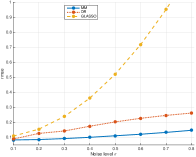
(a) Behaviour of rmse wrt $\sigma$.

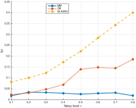
(b) Behaviour of fpr wrt $\sigma$.

Figure 2: Estimation results for different noise levels in terms of rmse (left) and fpr (right) for MM, GLASSO and DR approaches.

As expected, as the noise variance increases the reconstruction quality deteriorates. The GLASSO procedure is strongly impacted by the presence of noise, whereas the MM approach achieves better results, also when compared with DR algorithm. Moreover, the MM algorithm significantly outperforms both other methods in terms of support reconstruction, revealing itself very robust with respect to an increasing level of noise.

6 Conclusions

In this work, various proximal tools have been introduced to deal with optimization problems involving real symmetric matrices. We have focused on the variational framework (1) which is closely related to the computation of a proximity operator with respect to a Bregman divergence. It has been assumed that $f$ in (3) is a convex spectral function, and $g$ reads as $g_{0}+g_{1}$, where $g_{0}$ is a spectral function. We have given a fully spectral solution in Section 2 when $g_{1}\equiv 0$, and, in particular, 1 could be useful for developing algorithms involving proximity operators in other metrics than the Frobenius one. When $g_{1}\not\equiv 0$, a proximal iterative approach has been presented, which is grounded on the use of the Douglas–Rachford procedure. As illustrated by the tables of proximity operators provided for a wide range of choices for $f$ and $g_{0}$, the main advantage of the proposed algorithm is its great flexibility. The proposed framework also has allowed us to propose a nonconvex formulation of the precision matrix estimation problem arising in the context of noisy graphical lasso. The nonconvexity of the obtained objective function has been cirmcumvented through a Majorization–Minimization approach, each step of which consists of solving a convex problem by a Douglas-Rachford sub-iteration.

Comparisons with state–of–the–art solutions have demonstrated the robustness of the proposed method.

It is worth mentioning that all the results presented in this paper can be easily extended to complex Hermitian matrices.

References

- (1) Aragón Artacho, F.J., Borwein, J.M.: Global convergence of a non-convex Douglas–Rachford iteration. J. Global Optim. 57(3), 753–769 (2013). DOI 10.1007/s10898-012-9958-4
- (2) Aslan, M.S., Chen, X.W., Cheng, H.: Analyzing and learning sparse and scale-free networks using Gaussian graphical models. J. Mach. Learn. Res. 1(2), 99–109 (2016). DOI 10.1007/s41060-016-0009-y
- (3) Banerjee, O., El Ghaoui, L., d’Aspremont, A.: Model selection through sparse maximum likelihood estimation for multivariate Gaussian or binary data. J. Mach. Learn. Res. 9, 485–516 (2008)
- (4) Bauschke, H.H., Borwein, J.M., Combettes, P.L.: Essential smoothness, essential strict convexity, and Legendre functions in Banach spaces. Comm. Contemp. Math 3, 615–647 (2001)
- (5) Bauschke, H.H., Borwein, J.M., Combettes, P.L.: Bregman monotone optimization algorithms. SIAM J. Control Optim. 42(2), 596–636 (2003). DOI 10.1137/S0363012902407120
- (6) Bauschke, H.H., Combettes, P.L.: Convex Analysis and Monotone Operator Theory in Hilbert Spaces, 2nd edn. Springer International Publishing (2017). DOI 10.1007/978-3-319-48311-5
- (7) Bauschke, H.H., Combettes, P.L., Noll, D.: Joint minimization with alternating Bregman proximity operators. Pac. J. Optim. 2(3), 401–424 (2006)
- (8) Benfenati, A., Ruggiero, V.: Inexact Bregman iteration with an application to Poisson data reconstruction. Inverse Problems 29(6), 1–32 (2013)
- (9) Benfenati, A., Ruggiero, V.: Inexact Bregman iteration for deconvolution of superimposed extended and point sources. Commun. Nonlinear Sci. Numer. Simul. 20(3), 882 – 896 (2015). DOI http://dx.doi.org/10.1016/j.cnsns.2014.06.045
- (10) Bengtsson, I., Zyczkowski, K.: Geometry of Quantum States: An Introduction to Quantum Entanglement. Cambridge University Press, Cambridge (2006). DOI 10.1017/CBO9780511535048
- (11) van den Berg, E., Friedlander, M.P.: Probing the Pareto frontier for basis pursuit solutions. SIAM J. Sci. Comput. 31(2), 890–912 (2009). DOI 10.1137/080714488
- (12) Borwein, J., Lewis, A.: Convex Analysis and Nonlinear Optimization. Springer (2014)
- (13) Boyd, S., Parikh, N., Chu, E., Peleato, B., Eckstein, J.: Distributed optimization and statistical learning via the alternating direction method of multipliers. Found. Trends Mach. Learn. 3(1), 1–122 (2011). DOI 10.1561/2200000016
- (14) Bregman, L.M.: The Relaxation Method of Finding the Common Point of Convex Sets and Its Application to the Solution of Problems in Convex Programming. USSR Computational Mathematics and Mathematical Physics 7, 200–217 (1967)
- (15) Brune, C., Sawatzky, A., Burger, M.: Primal and dual Bregman methods with application to optical nanoscopy. Int. J. Comput. Vis. 92(2), 211–229 (2011). DOI 10.1007/s11263-010-0339-5
- (16) Burger, M., Sawatzky, A., Steidl, G.: First Order Algorithms in Variational Image Processing, pp. 345–407. Springer International Publishing, Cham (2016). DOI 10.1007/978-3-319-41589-5˙10
- (17) Cai, J.F., CandÚs, E.J., Shen, Z.: A singular value thresholding algorithm for matrix completion. SIAM J. Optim. 20(4), 1956–1982 (2010). DOI 10.1137/080738970
- (18) Cai, T., Liu, W., Luo, X.: A constrained minimization approach to sparse precision matrix estimation. J. Am. Stat. Assoc. 106(494), 594–607 (2011). DOI 10.1198/jasa.2011.tm10155
- (19) Chandrasekaran, V., Parrilo, P.A., Willsky, A.S.: Latent variable graphical model selection via convex optimization. Ann. Statist. 40(4), 1935–1967 (2012). DOI 10.1214/11-AOS949
- (20) Chartrand, R.: Nonconvex splitting for regularized low-rank + sparse decomposition. IEEE Trans. Signal Process. 60, 5810–5819 (2012)
- (21) Chaux, C., Combettes, P.L., Pesquet, J.C., Wajs, V.R.: A variational formulation for frame-based inverse problems. Inverse Problems 23(4), 1495 (2007)
- (22) Chaux, C., Pesquet, J.C., Pustelnik, N.: Nested iterative algorithms for convex constrained image recovery problem. SIAM J. Imaging Sci. 2(2), 730–762 (2009)
- (23) Chouzenoux, E., Pesquet, J.C.: Convergence Rate Analysis of the Majorize-Minimize Subspace Algorithm. IEEE Signal Process. Lett. 23(9), 1284 – 1288 (2016). DOI 10.1109/LSP.2016.2593589
- (24) Combettes, P.L., Pesquet, J.C.: A Douglas-Rachford splitting approach to nonsmooth convex variational signal recovery. IEEE J. Sel. Topics Signal Process. 1(4), 564–574 (2007)
- (25) Combettes, P.L., Pesquet, J.C.: Proximal Splitting Methods in Signal Processing. In: Fixed-Point Algorithms for Inverse Problems in Science and Engineering, pp. 185–212. Springer (2011). DOI 10.1007/978-1-4419-9569-8
- (26) Condat, L.: Fast projection onto the simplex and the ball. Math. Programm. 158(1), 575–585 (2016). DOI 10.1007/s10107-015-0946-6
- (27) Corless, R.M., Gonnet, G.H., Hare, D.E.G., Jeffrey, D.J., Knuth, D.E.: On the Lambert W function. Adv. Comput. Math. 5(1), 329–359 (1996). DOI 10.1007/BF02124750
- (28) Cover, T., Thomas, J.: Elements of Information Theory. A Wiley-Interscience publication. Wiley (2006)
- (29) d’Aspremont, A., Banerjee, O., Ghaoui, L.E.: First-order methods for sparse covariance selection. SIAM J. Matrix Anal. Appl. 30(1), 56–66 (2008). DOI 10.1137/060670985
- (30) Dempster, A.: Covariance selection. Biometrics 28, 157–175 (1972)
- (31) Duchi, J.C., Gould, S., Koller, D.: Projected Subgradient Methods for Learning Sparse Gaussians. In: UAI 2008, Proceedings of the 24th Conference in Uncertainty in Artificial Intelligence, Helsinki, Finland, July 9-12, 2008, pp. 145–152 (2008)
- (32) Friedman, J., Hastie, T., Tibshirani, R.: Sparse inverse covariance estimation with the graphical lasso. Biostatistics 9(3), 432–441 (2008). DOI 10.1093/biostatistics/kxm045
- (33) Goldstein, T., Osher, S.: The split Bregman method for l1-regularized problems. SIAM J. Imaging Sci. 2(2), 323–343 (2009). DOI 10.1137/080725891
- (34) Guo, J., Levina, E., Michailidis, G., Zhu, J.: Joint estimation of multiple graphical models. Biometrika 98(1), 1 (2011). DOI 10.1093/biomet/asq060
- (35) Hardy, G., Littlewood, J., Pólya, G.: Inequalities. Cambridge Mathematical Library. Cambridge University Press (1952)
- (36) Hunter, D.R., Lange, K.: A tutorial on MM algorithms. Amer. Statist. 58(1), 30–37 (2004). DOI 10.1198/0003130042836
- (37) Jacobson, M.W., Fessler, J.A.: An expanded theoretical treatment of iteration-dependent majorize-minimize algorithms. IEEE Trans. Image Process. 16(10), 2411–2422 (2007). DOI 10.1109/TIP.2007.904387
- (38) Komodakis, N., Pesquet, J.C.: Playing with duality: An overview of recent primal–dual approaches for solving large-scale optimization problems. IEEE Signal Process. Mag. 32(6), 31–54 (2015). DOI 10.1109/MSP.2014.2377273
- (39) Lewis, A.S.: Convex analysis on the Hermitian matrices. SIAM J. Optim. 6(1), 164–177 (1996). DOI 10.1137/0806009
- (40) Li, G., Pong, T.K.: Douglas–Rachford splitting for nonconvex optimization with application to nonconvex feasibility problems. Math. Programm. 159(1), 371–401 (2016). DOI 10.1007/s10107-015-0963-5
- (41) Li, L., Toh, K.C.: An inexact interior point method for –regularized sparse covariance selection. Math. Program. Comput. 2(3), 291–315 (2010). DOI 10.1007/s12532-010-0020-6
- (42) Lions, P.L., Mercier, B.: Splitting algorithms for the sum of two nonlinear operators. SIAM J. Numer. Anal. 16(6), 964–979 (1979). DOI 10.1137/0716071
- (43) Lu, Z.: Smooth optimization approach for sparse covariance selection. SIAM J. Optim. 19(4), 1807–1827 (2009). DOI 10.1137/070695915
- (44) Lu, Z.: Adaptive first-order methods for general sparse inverse covariance selection. SIAM J. Matrix Anal. Appl. 31(4), 2000–2016 (2010). DOI 10.1137/080742531
- (45) Ma, S., Xue, L., Zou, H.: Alternating direction methods for latent variable Gaussian graphical model selection. Neural Comput. 25(8), 2172–2198 (2013). DOI 10.1162/NECO˙a˙00379
- (46) Magnus, J.R., Neudecker, H.: Matrix Differential Calculus with Applications in Statistics and Econometrics, second edn. John Wiley (1999)
- (47) Marshall, A.W., Olkin, I., Arnold, B.C.: Inequalities: Theory of Majorization and its Applications, vol. 143, second edn. Springer (2011). DOI 10.1007/978-0-387-68276-1
- (48) Mazumder, R., Hastie, T.: The graphical lasso: New insights and alternatives. Electron. J. Stat. 6, 2125–2149 (2012). DOI 10.1214/12-EJS740
- (49) Meinshausen, N., Bühlmann, P.: High-dimensional graphs and variable selection with the lasso. Ann. Statist. 34(3), 1436–1462 (2006). DOI 10.1214/009053606000000281
- (50) Moreau, J.: Proximité et dualité dans un espace hilbertien. Bull. Soc. Math. France 93, 273–299 (1965)
- (51) Nesterov, Y.: Smooth minimization of non-smooth functions. Math. Programm. 103(1), 127–152 (2005). DOI 10.1007/s10107-004-0552-5
- (52) Parikh, N., Boyd, S.: Proximal algorithms. Found. Trends Optim. 1(3), 127–239 (2014). DOI 10.1561/2400000003
- (53) Pesquet, J.C., Pustelnik, N.: A parallel inertial proximal optimization method. Pac. J. Optim. 8(2), 273–305 (2012)
- (54) Ravikumar, P., Wainwright, M.J., Raskutti, G., Yu, B.: High-dimensional covariance estimation by minimizing -penalized log-determinant divergence. Electron. J. Statist. 5, 935–980 (2011). DOI 10.1214/11-EJS631
- (55) Richard, E., andre Savalle, P., Vayatis, N.: Estimation of simultaneously sparse and low rank matrices. In: Proceedings of the 29th International Conference on Machine Learning (ICML-12), pp. 1351–1358. ACM (2012)
- (56) Rockafellar, R.: Convex Analysis. Princeton landmarks in mathematics and physics. Princeton University Press (1970)
- (57) Rockafellar, R.T., Wets, R.J.B.: Variational Analysis, 1st edn. Springer-Verlag (1997)
- (58) Rothman, A.J., Bickel, P.J., Levina, E., Zhu, J.: Sparse permutation invariant covariance estimation. Electron. J. Statist. 2, 494–515 (2008). DOI 10.1214/08-EJS176
- (59) Scheinberg, K., Ma, S., Goldfarb, D.: Sparse inverse covariance selection via alternating linearization methods. In: Advances in Neural Information Processing Systems 23, pp. 2101–2109 (2010)
- (60) Sun, Y., Babu, P., Palomar, D.P.: Majorization-Minimization algorithms in signal processing, communications, and machine learning. IEEE Trans. Signal Process. 65(3), 794–816 (2017). DOI 10.1109/TSP.2016.2601299
- (61) Tipping, M.E.: Sparse Bayesian learning and the relevance vector machine. J. Mach. Learn. Res. 1, 211–244 (2001). DOI 10.1162/15324430152748236
- (62) Wang, C., Sun, D., Toh, K.C.: Solving log-determinant optimization problems by a Newton-CG primal proximal point algorithm. SIAM J. Optim. 20(6), 2994–3013 (2010). DOI 10.1137/090772514
- (63) Wipf, D.P., Rao, B.D.: Sparse Bayesian learning for basis selection. IEEE Trans. Signal Process. 52(8), 2153–2164 (2004). DOI 10.1109/TSP.2004.831016
- (64) Wu, C.F.J.: On the convergence properties of the EM algorithm. Ann. Statist. 11(1), 95–103 (1983). DOI 10.1214/aos/1176346060
- (65) Yang, S., Lu, Z., Shen, X., Wonka, P., Ye, J.: Fused multiple graphical lasso. SIAM J. Optim. 25(2), 916–943 (2015). DOI 10.1137/130936397
- (66) Yin, W., Osher, S., Goldfarb, D., Darbon, J.: Bregman iterative algorithms for -minimization with applications to compressed sensing. SIAM J. Imaging Sci. 1(1), 143–168 (2008). DOI 10.1137/070703983
- (67) Yuan, M., Lin, Y.: Model selection and estimation in the Gaussian graphical model. Biometrika 94(1), 19 (2007). DOI 10.1093/biomet/asm018
- (68) Yuan, X.: Alternating direction methods for sparse covariance selection (2009). URL http://www.optimization-online.org/DBFILE/2009/09/2390.pdf
- (69) Zangwill, W.I.: Nonlinear programming : a unified approach. Englewood Cliffs, N.J. : Prentice-Hall (1969)
- (70) Zhang, X., Burger, M., Bresson, X., Osher, S.: Bregmanized nonlocal regularization for deconvolution and sparse reconstruction. SIAM J. Imaging Sci. 3(3), 253–276 (2010). DOI 10.1137/090746379
- (71) Zhang, X., Burger, M., Osher, S.: A unified primal-dual algorithm framework based on Bregman iteration. J. Sci. Comput. 46(1), 20–46 (2011). DOI 10.1007/s10915-010-9408-8
- (72) Zhou, S., Xiu, N., Luo, Z., Kong, L.: Sparse and low-rank covariance matrices estimation (2014)