Block arrivals in the Bitcoin blockchain

Abstract

Bitcoin is a electronic payment system where payment transactions are verified and stored in a data structure called the blockchain. Bitcoin miners work individually to solve a computationally intensive problem, and with each solution a Bitcoin block is generated, resulting in a new arrival to the blockchain. The difficulty of the computational problem is updated every 2,016 blocks in order to control the rate at which blocks are generated. In the original Bitcoin paper, it was suggested that the blockchain arrivals occur according to a homogeneous Poisson process. Based on blockchain block arrival data and stochastic analysis of the block arrival process, we demonstrate that this is not the case. We present a refined mathematical model for block arrivals, focusing on both the block arrivals during a period of constant difficulty and how the difficulty level evolves over time.

I Introduction

Bitcoin is an electronic currency and payment system which allows for monetary transactions without a central authority. Bitcoin was first proposed in a white paper [1] in 2008 by the pseudonymous Satoshi Nakamoto, and as a functioning open source software system in January 2009. Since then it has grown rapidly and now has a market capitalisation of over US$160 billion.

The stated benefits of Bitcoin relative to payment over the Internet with traditional currencies include immutable transactions, relative anonymity, freedom against seizure by a central authority, faster and cheaper international currency transfer, among others. The technology used in Bitcoin also has potential to be applied to a wider range of applications including identity management, distributed certification and smart contracts.

Bitcoin employs a peer-to-peer network of nodes, computers which verify, propagate and store information about bitcoin transactions. Bitcoin maintains a global ledger of all Bitcoin transactions ever conducted – the Bitcoin blockchain – distributed over the network of Bitcoin nodes. The problems of maintaining and updating a global ledger without a trusted central authority, while still allowing any owner of bitcoins to spend them as they wish are solved by a series of cryptographic techniques. The technique of central interest for this paper is proof-of-work, whereby those who wish to contribute to building a consensus about which transactions are included in the ledger must perform some computational “work”. This work is referred to as Bitcoin mining.

Bitcoin users conduct transactions by cryptographically signing messages, which identify who is to be debited, who is to be credited, and where the change (if any) is to be deposited. These messages are then propagated through the Bitcoin network before being added to the blockchain. Each node in the network keeps a list of valid outstanding transactions called the transaction pool and passes it to neighbours in the network. Before a transaction can be included in the blockchain, a new block containing that transaction must be mined. A block is a list of transactions, together with metadata including the current time and a reference to the most recent previous block in the blockchain (hence the name blockchain). A block also includes a field called a nonce. The nonce contains no information, so it can be freely varied in an attempt to find a valid block that satisfies the requirements of the blockchain. To find such a block and publish it to the bitcoin network is referred to as mining a block.

I-A Bitcoin mining

Mining is a race between all the Bitcoin miners to find a valid block to append to the blockchain. To have a good chance of winning this race requires substantial computational resources, and the reward for doing so is a bounty of (currently 12.5) new bitcoins.

The requirements for a block to be valid are based on Bitcoin’s hash function. In general, a hash function $f$ maps a string $s$ (or equivalently, an integer, if the binary representation of the string is interpreted as an integer in base 2) to another string (integer) $f(s)$, the hash of $s$. The key property of the hash functions used in Bitcoin is that given any $y$ in the codomain of $f$ it is computationally infeasible to find any element of $f^{-1}(y)$. Furthermore, the hash functions are designed such that any change in the input string $s$ results in a totally different output $f(s)$. That is, $f(s_{1})$ gives no information about $f(s_{2})$ if $s_{1}\neq s_{2}$, and so to calculate hashes for a large number of input strings requires calculating each hash separately. This property allows hashes to act as short, tamper-proof summaries of large data files. Calculating the hashes of large numbers of arguments $s$ is the computational work in Bitcoin’s proof-of-work.

A Merkle tree is used to summarise and verify the integrity of the transactions in a block.The Merkle tree is constructed by recursively hashing pairs of transactions until there is only one hash, called the Merkle root. The block header is formed from the Merkle root, metadata (including the hash of the previous block) and the nonce. For a block to be valid the hash of the block header must be less than a certain value $L$, referred to as the target. The hash of the candidate block is calculated. In the rare case that the hash is less than the current target $L$, the block is valid and is appended to the miner’s blockchain: the block is said to have been mined. In the far more likely case that the hash is not less than the current target, the nonce is changed and the hash is recomputed. This process is repeated (occasionally updating metadata or the list of transactions) until some miner finds and publishes a block. When a block is mined it is broadcast to all the other miners who append the new block to their blockchains and resume mining “on top of” the new block.

Bitcoin’s hash function maps $\mathbb{Z}^{+}\cup\{0\}$ to $\{0,1,\ldots,2^{256}-1\}$. The computational difficulty in mining arises because Bitcoin hashes are effectively uniformly distributed in the interval $(0,2^{256}-1)$ while the target $L$ is much much less than $2^{256}$. Consequently, the checking of a candidate block is a Bernoulli trial with a probability of $L/2^{256}$ of being successful. By design, this probability is at most $2^{-32}$. The trials are functionally independent, therefore the number of hashes that need to be checked before a valid block is found is a geometric random variable, with a very large mean, $2^{256}/L$ ($\approx 6.2\times 10^{21}$ at the time of writing). On the other hand, computers around the world are currently performing hash function calculations at a very large rate ($\approx 10^{19}$ hashes per second at the time of writing). The time taken to mine a block is therefore very well-modelled by an exponential random variable. Furthermore, over any time interval where we can take the rate of trials to be constant, the process whose events are given by the instants at which blocks are mined should be well-approximated by a Poisson process, with a rate given by the product of the number of hashes $H$ calculated per second globally (the global hash rate), the value $L$ of the target, and a constant.

The success of the blockchain method has resulted in Bitcoin becoming increasingly popular and inspiring other electronic payment methods and other systems, such as online education certification [2], that use blockchain mechanisms for verification purposes. Indeed, although we will focus on the Bitcoin blockchain, we point out that our analysis can apply to other systems where similar blockchain policies are used.

I-B Target (and difficulty) adjustment

The target $L$ does not remain constant: it is adjusted every 2,016 blocks in an attempt to maintain an average mining rate of 6 blocks per hour (2,016 blocks in 1,209,600 seconds) despite changes in the amount of computational power being used for mining. Let $X_{n}$ be the time (in seconds) at which the $n^{\mathrm{th}}$ block is mined and define $X_{0}=0$. Then the target is adjusted at times $X_{2016i}$ for $i=1,2,\ldots$. We call the time between adjustments of the target a segment. Let the target in the $i^{\mathrm{th}}$ segment $(X_{2016(i-1)},X_{2016i})$ be $L_{i}$. Then

$$L_{i+1}=L_{i}{(X_{2016i}-X_{2016(i-1)})}/{1209600}$$ (1)

where $L_{0}=2^{224}$. If $X_{2016i}-X_{2016(i-1)}$ is shorter than two weeks, the target $L$ is reduced proportionally, and the average number of hashes checked to mine a block is increased, slowing down mining. A common variable used instead of the target is the difficulty $D$ defined as

$$D_{i} =\frac{2^{224}}{L_{i}}=D_{i-1}\frac{1209600}{(X_{2016i}-X_{2016(i-1)}}$$ (2)

so that $D_{0}=1$. The difficulty $D$ is $2^{32}$ times the average number of hashes required to mine a block (see Equation (22)), and denotes how much harder it is to mine a block than with the original (maximum) target. This difficulty adjustment is part of what makes the block arrival process for Bitcoin interesting: the adjustment is a change in the block arrival rate based on the random block arrival process itself, and the adjustment also occurs at a random time.

I-C Related work

Nakamoto [1] did not explicitly state that the blocks arrive according to a homogeneous Poisson process. However, the calculations in [1] are based on the assumption that the number of blocks that an attacker, mining at rate $\lambda_{1}$, mines in the expected time $z/\lambda_{2}$ that it takes for the community to mine $z$ blocks at rate $\lambda_{2}$, is Poisson with parameter $\lambda_{1}z/\lambda_{2}$, which is essentially equivalent to a Poisson process assumption. Rosenfeld [3] pointed out that, under the assumption that blocks arrive in a Poisson process, the number of blocks created by an attacker in the time that it takes the community to create a fixed number of blocks is a random variable with a negative binomial distribution; see also [4, Section 1.4]

Rosenfeld also assumed that the block arrival process is a Poisson process in [5] where he analysed reward structures for pooled Bitcoin mining with a view to reducing the variance in miner rewards while retaining fairness and preventing miners from being incentivised to hop between pools. Lewenberg et al. [6] also used a Poisson process model when they addressed a similar problem, although unlike Rosenfeld they took a game theory perspective and incorporated a constant, deterministic value of the block propagation delay.

Eyal and Sirer [7] proposed an attack strategy called selfish-mine, where certain dishonest miners keep discovered blocks private in the hope that they can gain larger rewards than honest miners. The majority of analysis on this topic has explicitly or implicitly assumed a Poisson process model for the block mining process, and typically used a Markov chain model for the number of blocks mined by the selfish mining pool and those mined by the rest of the miners. Sapirshtein et al. [8] found the optimal strategy for performing selfish mining. Göbel et al. [4] performed a stochastic and simulation analysis of the selfish-mine strategy in the presence of propagation delay.

A Poisson process assumption for the block arrival process has been used in other work. For example, Solat and Potop-Butucaru [9] assumed a (homogeneous) Poisson process for the block arrivals in their paper, where they developed a timestamp-free method for combating attacks such as selfish-mine, although this method does not crucially rely upon the Poisson assumption. Decker and Wattenhofer assumed a (homogeneous) Poisson process over periods where the difficulty is constant in their analysis of the propagation of transactions and blocks through the Bitcoin network [10]. Miller and LaViola[11] also assumed a Poisson process when modelling the Bitcoin system as a means of reaching fault-tolerant consensus.

I-D The goal and structure of the paper

Despite the analyses mentioned in Section 1.3 above, there has been little research to examine whether the block arrival process in the Bitcoin blockchain actually does behave like a homogeneous Poisson process.

The goal of this paper is to examine this assumption. It will turn out that, at certain timescales, the block arrival process is not Poisson, which will motivate us to propose refined point process models for the block arrival process. We present a suite of point process models for the block generation process, suitable for viewing the process over a range of different timescales. Over long timescales, this comes down to fitting time-varying models to the hash rate. Over shorter timescales we need to take into account the dependencies introduced by the difficulty update mechanism and the fact that the hash rate is varying within each segment while the difficulty remains constant.

Our work here differs from previous modelling of the Bitcoin blockchain because the difficulty adjustment is taken into account, and we also examine the consequences of the interaction between the block propagation delay and the hash rate upon the blockchain process. We also infer miner-to-miner propagation delay from the available block timestamp data.

The rest of the paper is structured as follows. In Section II we discuss the data available on the Bitcoin blockchain and their limitations. In Section III we explain the drivers of the global hash rate, and how to estimate the hash rate from the available data. In Section IV we discuss several models for the block arrival process, including how to approximate the hash rate in order to allow more tractable analysis of the desired model. We present results on the behaviour of the Bitcoin system, and give a deterministic approximation. Section V presents a summary of our various block arrival models. Section VI presents the results of a simulation of the Bitcoin blockchain. We summarise our results in Section VII.

II The block arrival process: the data

Blocks arrive, that is, they are mined, published to the bitcoin network and are added to the blockchain according to a random process. Examining the block arrival process can serve as a means of diagnosing the health of the blockchain, as well as detecting the actions of malicious entities.

There are several ways in which we can define when a block “arrives”. The two that are easiest to measure are:

1. the time when the block arrives at our measurement node (or nodes), and

2. the timestamp encoded in the block header.

There are advantages and disadvantages associated with each of these methods. We have forthcoming work on estimating the distribution of errors in the arrival times from the combination of both sources of data.

II-A Block arrival times

The time when a block arrives at any given node in the Bitcoin peer-to-peer network depends upon when the block was mined and how the block propagates through the peer-to-peer network. While propagation adds a random delay component to the time when the block was mined, it also represents when a block can truly be said to have arrived at the node. Once a block has propagated through the network (and to our measurement nodes), then the information contained within the block is visible to to the miners and the users of Bitcoin, and it is much less likely that any miner will mine on top of a previous block and cause a conflict. However, a substantial problem with using block arrival times at measurement nodes is that it is impossible to get historical information, or information from periods when the measurement nodes were not functioning, or not connected to the network.

II-B Block timestamps

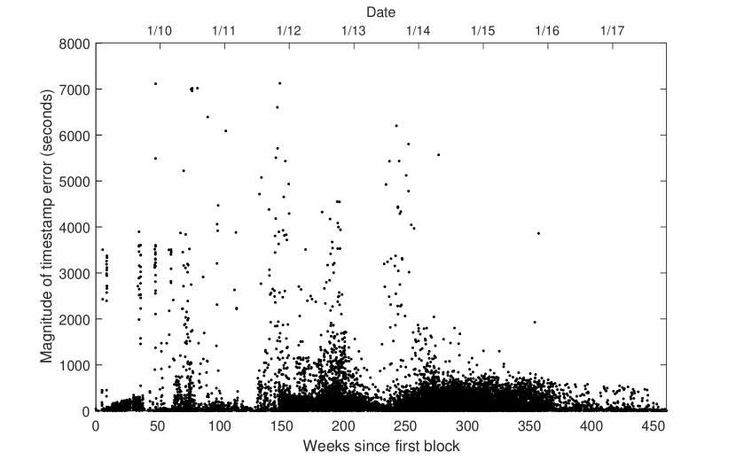
(a) Scatter plot of the sizes of the timestamp errors vs. when they occurred. Out-of-order timestamps are prevalent throughout the history of Bitcoin.

(b) Histogram of the sizes of the timestamp errors. The local peak at -1500 includes all pairs of adjacent blocks $i,i+1$ whose difference in timestamps $X_{i+1}-X_{i}<-1500$.

Figure 1: Known timestamp errors when timestamps for two consecutive blocks in the blockchain are out of order.

Using the timestamp in the block header as the authoritative time has its own disadvantages. This time is determined from the miner’s clock when the mining rig creates the block template. If the miner’s clock is incorrect then this will introduce an error. Timestamp errors are limited in magnitude: blocks with timestamps prior to the median timestamp of the previous 11 blocks, or more than 2 hours into the future are rejected as being invalid and will not be propagated by the network.

Nevertheless, block timestamp errors can be severe. For example, of the 500,000 blocks mined up to November 2017, 13,618 of them have a timestamp prior to that of the previous block and some 1,000 of them have timestamps more than 10 minutes prior to the previous block timestamp. If one considers that a miner has access to the previous block (and hence the timestamp of the previous block) before mining the next block, these errors seem particularly anomalous. This suggests that some miners intentionally use inaccurate timestamps. One potential reason for this is mining software that varies the timestamp to use it as an additional nonce.

Figure 1(a) shows a scatter plot of the magnitude of the negative inter-arrival times versus the timestamp at which they occurred. The horizontal axis covers the entire history of Bitcoin. These errors are not localised to specific times in history. Incorrect timestamps remain frequent even recently in the blockchain.

Figure 1(b) shows a truncated histogram of the sizes of the negative inter-arrival times. Some inter-arrival times are more negative than $-7,000$ seconds but most are between $-1,500$ and $0$ seconds.

We will later argue that while data for individual arrivals are unreliable, our estimation of the hash rate is insensitive to errors in the individual arrival times (especially if those errors are independent) since it only relies upon the average rate of arrival of large numbers of blocks.

II-C Cleaning the data

Blockchain timestamps are recorded in whole numbers of seconds since the 1st of January 1970, with the first block being mined on the 3rd of January 2009. The first step we took was to disregard all data prior to the 30th of December 2009. Owing to Bitcoin being newly adopted over 2009, the block arrival process in this period had a large number of anomalies, including one day in which no blocks were mined.

The next step was to deal with obvious errors. As discussed in Section II-B, it is possible to have errors in the timestamps. We know the order that the blocks must have been mined in, because each block header contains the hash of the previous block header. Let the timestamp of the $i^{\mathrm{th}}$ block be $X_{i}$. Due to errors, sometimes the timestamps are out of order: $X_{i}>X_{j}$ for some $i<j$. We call $T_{i}:=X_{i}-X_{i-1}$ the $i^{\mathrm{th}}$ inter-arrival time, and if $T_{i}$ is negative then there must have been an error. Some of these errors are both substantial and obvious: for instance if $X_{i}-X_{i-1}=7162$ and $X_{i+1}-X_{i}=-6603$ while other nearby inter-arrival times are unremarkable, then it would be sensible to assume that $X_{i}$ is an error. However, there are other cases that are more complicated to deal with. There are several approaches that we considered.

1. Ignore: Ignore the fact that the data are out of order. If we then look at the block inter-arrival times, some of these will be negative. Also, some will be very large. If we are studying the variance of the inter-arrival times then this will be inflated relative to any of the methods discussed below. Furthermore, the empirical distribution function for inter-arrival times will not make physical sense, and will certainly not be exponentially distributed.

2. Reorder: Sort the timestamps into ascending order. This results in non-negative inter-arrival times, but we are essentially removing random points and inserting them elsewhere in the process. This has a far from obvious effect, and the effect is dependent on the distribution of these already unreliable timestamps.

3. Resample: Remove those timestamps which we deem unreliable (by some criterion), then resample them uniformly in the interval between the adjacent timestamps that we consider reliable. For instance, say $X_{i+1},X_{i+2},X_{i+3}$ are deemed unreliable but $X_{i}$ and $X_{i+4}$ are not. Then we would independently uniformly sample three timestamps in the interval $(X_{i},X_{i+4})$, sort those new timestamps, and replace the previous values of $X_{i+1},X_{i+2},X_{i+3}$ by the three new timestamps. This is essentially replacing the unreliable timestamps with timestamps sampled from a Poisson process on $(X_{i},X_{i+4})$, conditional on there being three timestamps in this interval. There are a few ways we can determine which timestamps are unreliable:

   1. Try to guess which timestamps are unreliable based on the surrounding timestamps. It is not clear how to do this, especially if we wish to do it empirically.

   2. Declare any timestamp that is adjacent to a negative inter-arrival time to be unreliable. That is, if $X_{i+1}-X_{i}<0$, both $X_{i}$ and $X_{i+1}$ are unreliable.

   3. Sort the timestamps and consider any timestamp that changes position when sorted to be unreliable. This addresses the case of a single wrong timestamp the same way as in (3b) and provides a consistent approach for more complicated scenarios.

   4. Find the longest increasing subsequence of the data (if $X_{1},X_{2},\ldots$ is treated as a sequence). Such a subsequence might not be unique. If there is more than one longest increasing subsequence, then take the intersection of all longest increasing subsequences. Any timestamps not in this intersection are considered unreliable.

   Once the unreliable timestamps are determined, resample them between the adjacent reliable timestamps.

To see why (3d) is reasonable, consider the case of having two adjacent timestamps a long way out of order, see for instance Figure 2: $X_{1}<X_{2}<X_{5}<X_{6}<X_{7}<X_{8}<X_{3}<X_{4}$. This is a scenario that actually occurs in the blockchain. Here it is clear that $X_{3}$ and $X_{4}$ should be the timestamps under suspicion, but (3b) will replace $X_{4}$ and $X_{5}$, and (3c) will replace all of $X_{3},\ldots,X_{8}$, whereas (3d) replaces exactly $X_{3}$ and $X_{4}$. The algorithm for computing this is available at [12].

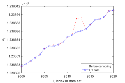
Figure 2: An example of the effect of the resampling scheme (3d) from Section II-C. The index $i$ is the number of blocks since 1 January 2009.

These are the steps we followed to clean the block arrival time data:

• Disregarded all data prior to the 30th of December 2009.

• Performed (3d) for the rest of the data.

We refer to the data after these two steps as LR (later, resampled). Of the 464,372 blocks after the 30th of December 2009, 441,225 or 95% of them are in every longest increasing subsequence. The remaining 5% were resampled. While the longest increasing subsequences span the whole length of the blockchain, the errors that are corrected by taking the intersection of all longest increasing subsequences are all of a local nature. Most of those timestamps that were resampled were in consecutive groups of 1, 2 or 3. Two consecutive timestamps being resampled was the most common: this occurs when one timestamp is incorrect but with a small enough error to be only one place out of order. The other timestamp that it is transposed with will also be considered unreliable and resampled. An isolated timestamp being resampled is caused by that timestamp having a particularly large error. If a timestamp has a large error it can have two or more timestamps between its observed value and its correct value. In this case, if none of the other nearby timestamps are out of order the incorrect timestamp will be the only one resampled.

We provide this data (along with annotation as to which points have been resampled) at [12]. We suggest that this sequence could serve as a reference version of cleaned blockchain timestamp data for other research on this topic.

III Estimating the global hash rate

The global hash rate $H(t)$ is a key factor driving the block arrival process. It is the total processing power (hashes calculated per second) that all the Bitcoin miners in the world are dedicating to mining at time $t$. In the long term, $H(t)$ is largely increasing exponentially in a Moore’s Law fashion. The main drivers of change in the hash rate are:

1. Miners switching new machines on. This typically involves ordering mining machines from one of a small number of ASIC manufacturers, often while those ASICs are still in development, and waiting for the manufacturer (who is prone to delays) to manufacture and ship the ASICs in batches. Then the ASICs arrive at the miners and they install them and switch them on and start mining. Each generation of new mining machines is faster than the last, although this increase is not steady, even in an exponential sense. It is widely believed that the rate of increase in the hash rate is petering out now.

2. Mining machines becoming uneconomical because of increasing electricity prices, increasing global hash rates, reduced bitcoin prices, or halving of the mining reward, and being switched off.

3. Mining machines becoming more economical due to both to technological advancements and, at times, the increasing value of bitcoins, and when electricity prices are reduced.

III-A Empirical estimates for the global hash rate

The global hash rate $H(t)$ cannot be measured directly. However, the difficulty $D_{i}$ is recorded in the header of every block. Equations (1) and (2) can be combined to give

$$D_{i+1}=\frac{1209600D_{i}}{X_{2016i}-X_{2016(i-1)}}.$$ (3)

The ratio $2016/(X_{2016i}-X_{2016(i-1)})$ is the average rate of block discovery in the period $[X_{2016i},X_{2016(i-1)})$, and $2^{32}D_{i}$ is the expected number of hashes that must be checked to find a valid solution when the difficulty is $D_{i}$. A reasonable estimate $\widehat{H}_{i}$ for the average of the global hash rate $H(t)$ over the segment $(X_{2016i},X_{2016(i-1)})$ is therefore given by the product of those two quantities, namely

$$\widehat{H}_{i}=\frac{2016\times 2^{32}D_{i}}{X_{2016i}-X_{2016(i-1)}}=\frac{2^{32}}{600}D_{i+1}.$$ (4)

Thus we can get a sense of how the hash rate has changed over time by examining the graph of the difficulty over time presented in Figure 3.

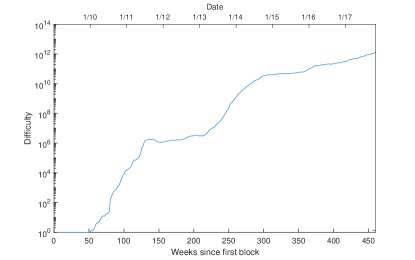
Figure 3: Plot of the difficulty over the life of the blockchain. This serves as an estimate of a constant multiple of the global hash rate.

We can refine this approach to obtain a sliding window estimate $H^{W}_{k,i}$ of the hash rate, with the window being fixed at $k$ blocks long, centred around the $i^{\mathrm{th}}$ block.

$$H^{W}_{k,i}=\frac{2^{32}}{X_{\lceil i+k/2\rceil}-X_{\lceil i-k/2\rceil}}\sum_{j=\lceil i+k/2\rceil}^{\lceil i-k/2\rceil}D_{\lceil j/2016\rceil}.$$ (5)

If there was no difficulty change between $X_{\lceil i+k/2\rceil}$ and $X_{\lceil i-k/2\rceil}$, then

$$H^{W}_{k,i}=\frac{2^{32}D_{\lceil i/2016\rceil}k}{X_{\lceil i+k/2\rceil}-X_{\lceil i-k/2\rceil}}.$$ (6)

We can consider $H^{W}_{k,i}$ to be an estimate of $H(t)$ at times $t_{i}=(X_{\lceil i+k/2\rceil}+X_{\lceil i-k/2\rceil})/2$. To get a continuous estimator we can linearly interpolate between these points to get $H^{W}_{k}(t)$ for $t\geq X_{k/2}$.

The estimation of $H(t)$ from Equation (5) is not without its problems due to the stochastic nature of the block arrival process, and inaccuracies in the values of the block timestamps $X_{i}$. If the window $k$ is longer, there is less stochastic variation in the estimate, but the time resolution of the resulting estimate of $H(t)$ is lower so that it is more difficult to pick up short-term fluctuations in $H(t)$, yielding the standard bias/variance trade-off when performing smoothing. Note that regardless of what window we use, the time resolution of the estimate will be limited by the frequency of block arrivals, and the noise caused by the stochastic variation inherent in the process.

Another method for estimating $H(t)$ via smoothing the block arrival data is by using a method essentially equivalent to weighted kernel density estimation (KDE), but without the requirement that the output is a density. For each block $i=1,2,\ldots$ we centre a kernel $K(x)$ at the measured time $X_{i}$ of the arrival of the block, and weight it with $w_{i}=2^{32}D_{\lceil i/2016\rceil}$ where $w_{i}$ is the number of hashes that must be checked on average to mine a block with the same difficulty as block $i$. The kernel estimator is given by

$$H^{K}_{h}(t) =\frac{1}{h}\sum_{i}w_{i}K({(t-X_{i})}/{h})$$

$$=\frac{2^{32}}{h}\sum_{i}D_{\lceil i/2016\rceil}K({(t-X_{i})}/{h}).$$ (7)

Some examples of appropriate kernel functions are the rectangular function $K(x)=\frac{1}{2}1_{|x|<1}$, the normal density function $\frac{1}{\sqrt{2\pi}}e^{-x^{2}/2}$, and the Epanechnikov kernel [13] $\frac{3}{4}(1-x^{2})1_{|x|<1}$. Here $h$ is referred to as the bandwidth of the kernel estimator. The bandwidth $h$ performs a role similar to that of the window size $k$ above, so the value of $h$ is important. If $h$ is too small then the data has spurious variability from measurement error (and more substantially, from the stochastic variability of block discoveries). If $h$ is too large then the data will be oversmoothed and fail to capture true short-term variability in $H(t)$. However, we are primarily interested in the long term behaviour of $H(t)$, so our conclusions later in the paper are relatively insensitive to which estimate for $H(t)$ we use, the kernel function $K(x)$ and the window size $k$ or the bandwidth $h$.

Figure 4 shows a comparison of $H^{W}_{144}(t)$, $H^{W}_{2016}(t)$, $H^{K}_{\texttt{1 day}}(t)$, $H^{K}_{\texttt{2 weeks}}(t)$ and $H^{K}_{6\texttt{ months}}(t)$ over the life of the Bitcoin blockchain where $K$ denotes the Epanechnikov kernel. At this scale it is difficult to distinguish between $H^{W}_{2016}(t)$ and $H^{K}_{\texttt{2 weeks}}(t)$. The more smoothed kernel-based estimate ($h=6\texttt{ months}$) appears to lead the other estimates because the rapid increase in the hash rate is dispersed by the width of the kernel into the time before it has truly happened. This makes the smoother (higher bandwidth) estimate misleading and we will use a lower bandwidth estimate for the remainder of the paper. The behaviour of the blockchain in the first 50 weeks is erratic.

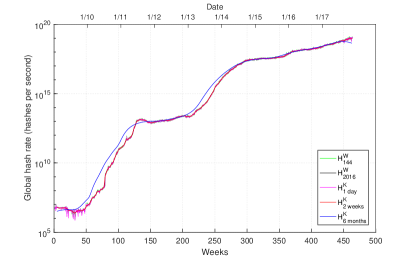
Figure 4: Estimates of the hash rate $H^{W}_{2016}(t)$, $H^{W}_{144}(t)$, $H^{K}_{\texttt{1 day}}(t)$, $H^{K}_{\texttt{2 weeks}}(t)$ and $H^{K}_{6\texttt{ months}}(t)$ respectively from January 2009 to April 2017. The sliding window estimate with $k=2016$ is not identical to the kernel-based estimate with $h=\texttt{2 weeks}$, but it is almost indistinguishable at this scale, so the two curves overlay and only one of them is visible on the graph.

III-B Intervals of exponential growth in the global hash rate

By inspecting the plot of an estimate of the hash rate from 2009 to 2017 (Figure 4) we see that the logarithm of the global hash rate is approximately linear for long periods, that is, the hash rate is increasing exponentially. We approximate the global hash rate $H(t)$ by $e^{at+b}$ on intervals where it can be estimated that $a$ and $b$ remain constant. In Figure 5 we partition the history of the blockchain into such periods, and for each of these periods we fit a linear function to $\log(H^{W}_{144}(t))$ using standard linear regression. The values for this fit are given in Table I.

interval	start	end	$a$	$b$
1	3 Jan 2009	30 Dec 2009	$-9.44\times 10^{-9}$	27.1
2	30 Dec 2009	13 Jul 2010	$2.18\times 10^{-7}$	-259
3	13 Jul 2010	24 Jun 2011	$2.72\times 10^{-7}$	-326
4	24 Jun 2011	1 Mar 2013	$2.01\times 10^{-8}$	3.38
5	1 Mar 2013	9 Oct 2014	$1.96\times 10^{-7}$	-236
6	9 Oct 2014	24 Nov 2017	$3.88\times 10^{-8}$	-15.1

Table I: The parameters of the piecewise exponential hash rate $\widehat{H}(t)=e^{at+b}$ in each interval, with $t$ in seconds. Each interval starts and ends on a segment boundary.

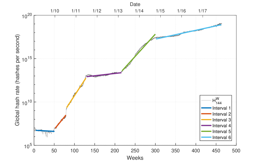
(a) All intervals

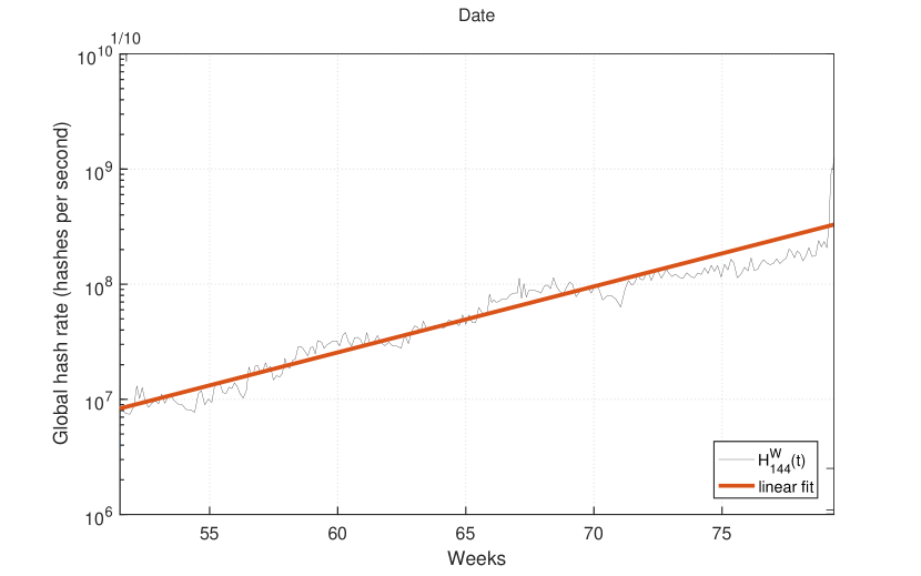
(b) Interval 2

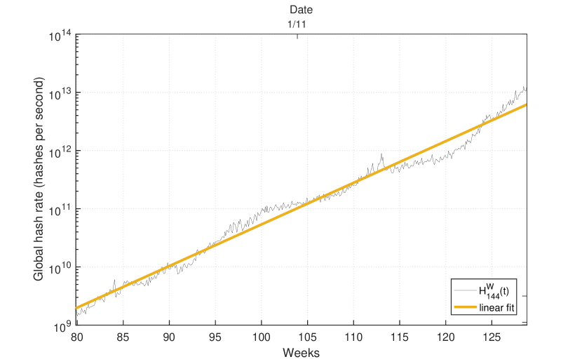
(c) Interval 3

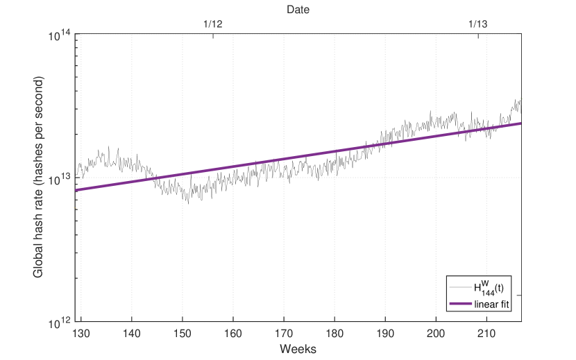
(d) Interval 4

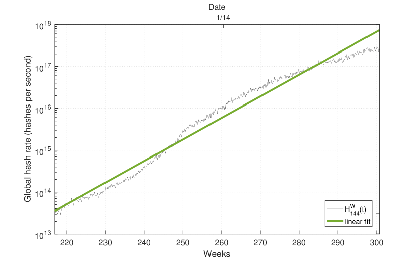
(e) Interval 5

(f) Interval 6

Figure 5: Linear fits to $H^{W}_{144}(t)$ over a sequence of six intervals, with the endpoints of the intervals given in Table I. A closer view of the fitted hash rate $\widehat{H}(t)=e^{at+b}$ and a more fine-grained estimate of the hash rate $H^{W}_{144}(t)$ over the intervals is given in subfigures (b) through (f).

The assumption of exponential growth in the hash rate is natural for two reasons. First, the increase in Bitcoin mining power is partially driven by technological developments: the processors used in mining have become increasingly cost- and energy-efficient over time in a manner reminiscent of Moore’s Law. Second, we observe in the actual blockchain that the average time taken for a segment is consistently under 2 weeks. If we want the average time taken for a segment to be stationary with a mean not equal to 2 weeks then $H(t)$ is required to grow exponentially. Intuitively, if the time taken for each segment was roughly constant at a value of $T_{2016}$, then the difficulty $D(t)$ would increase by a factor of $({\texttt{2 weeks}})/T_{2016}$ each segment, and since the difficulty is increasing exponentially, the hash rate would also have to increase exponentially to maintain constant segment time. Approximating $\log(H(t))$ with a linear function also has the benefit of tractability for modelling and analysis.

We can calculate the limiting average for segment times by recognizing that the average change in the difficulty of successive segments is cancelled out by the growth in the hash rate over the duration of each segment. The faster the increase in the hash rate, the lower the limiting average inter-arrival time.

Let $\widehat{H}(t)=e^{at+b}$. Then the multiplicative growth in hash rate over a segment of duration $T_{2016}$ is $e^{aT_{2016}}$. The ratio of the new difficulty to the previous difficulty, given by Equation (3), is $(\texttt{2 weeks})/T_{2016}$. In seconds, this gives the relationship between the average time taken to mine a segment and the slope of the logarithm of the hash rate (see Equation (35))

$$e^{aT_{2016}}=1209600/T_{2016}$$ (8)

or equivalently,

$$a=\frac{1}{T_{2016}}\log\left({1209600}/{T_{2016}}\right).$$ (9)

Note that the long-term average time to mine a block is $T_{2016}/2016$, although the average inter-arrival time decreases over the course of each segment as shown in Figure 7 below. This means that the long-term average time to mine a block $T_{\texttt{ave}}$ when the hash rate is $H(t)=e^{at+b}$ is given by solving the relationship

$$e^{2016aT_{\texttt{ave}}}=600/T_{\texttt{ave}}.$$ (10)

We simulated the arrival of 40,000 blocks with random difficulty changes (exponential hash rate function, no block propagation delay) using a range of values of $a$. Figure 6 shows that the long term average block inter-arrival time agrees with Equations (8) through (10). Further, we also plot the average inter-arrival time of the observed blockchain timestamp data for each of the intervals in Table I versus the fitted value of $a$ for each interval. Figure 6 shows that the observed data also fits the predicted relationship in Equation (8). We provide a theoretical basis for Equation (8) in Section IV-D2.

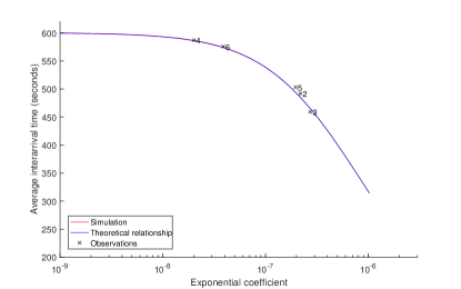
Figure 6: The relationship between the inter-arrival time and $a$, the slope of the logarithm of the hash rate over time, in theory, simulations and observations. The global hash rate at time $t$ is modelled by $\widehat{H}(t)=e^{at+b}$. The system reaches a steady state where the average time $T_{\texttt{ave}}$ for a block to arrive is related to $a$ by Equation (10). The simulated values are given by a simulation of 40,000 blocks with exponential hash rate, random difficulty changes and no propagation delay. The observed values of the average inter-arrival time are calculated from the observed timestamps for each interval, and the values of $a$ are the fitted values given in Table I. The segment time is 2016 times the average block inter-arrival time for the relevant interval.

IV Is the block arrival process a Poisson process?

IV-A Poisson processes

A point process $N$ is a Poisson point process on $\mathbb{R}$ if it has the following two properties [14, Chapter 2.4].

1. The random number of points $N([a,b))$ of the point process $N$ located in a bounded interval $[a,b)\subset\mathbb{R}$ is a Poisson random variable with mean $\Lambda([a,b))$, where $\Lambda$ is a non-negative Radon measure.

2. The numbers of points of the point process $N$ located in $k$ intervals $[a_{1},b_{1}),\dots,[a_{k},b_{k})$ form $k$ independent Poisson random variables with means $\Lambda([a_{1},b_{1})),\dots,\Lambda([a_{k},b_{k}))$.

From now on we will write $N([a,b))$ as $N(a,b)$ and $\Lambda([a,b))=\Lambda(a,b)$ for convenience. The first property implies that

$$\mathbb{P}(N(a,b)=n)=\frac{\Lambda(a,b)^{n}\textrm{e}^{-\Lambda(a,b)}}{n!},$$ (11)

and $\mathbb{E}[N(a,b)]=\Lambda(a,b)$, while the second property is the principal reason for the tractability of the Poisson point process and it is usually the basis of statistical tests that measure the suitability of Poisson models. The Poisson distribution of $N(a,b)$ implies its variance is $\mathrm{Var}[N(a,b)]=\Lambda(a,b)$, a fact that is also used as a statistical test.

The measure $\Lambda$ is known as the intensity measure or mean measure of the Poisson point process. We will assume that a function $\lambda(t)$ exists such that

$$\Lambda(a,b)=\int_{a}^{b}\lambda(t)\textrm{d}t.$$ (12)

Then $\lambda(t)$ is known as a rate function. If $\lambda(t)$ is a constant $\lambda>0$ then the point process is called a homogeneous Poisson point process. Otherwise, the point process is called an nonhomogeneous or inhomogeneous Poisson point process. Restricting our attention to the interval of non-negative numbers $[0,\infty)$, the intensity measure is given by

$$\Lambda(t):=\Lambda([0,t))=\int_{0}^{t}\lambda(t)\textrm{d}t,$$ (13)

For a Poisson process $N$ with intensity measure $\Lambda$, the probability of $n$ points existing in the interval $[a,b)$ is

$$\mathbb{P}(N(a,b)=n)=\frac{[\Lambda(b)-\Lambda(a)]^{n}\textrm{e}^{-[\Lambda(b)-\Lambda(a)]}}{n!}.$$ (14)

IV-A1 Arrival times and inter-arrival times

Consider a point process $\{X_{(i)}\}_{i\geq 1}$ defined on the non-negative reals with an almost certainly finite number of points in any bounded interval. Then we can interpret the points of the process as arrival times and put them in increasing order, $X_{1}\leq X_{2}\leq\ldots$. Then the distances between adjacent points are $T_{i}:=X_{i}-X_{i-1}$ for $i=2,3,\ldots$ and $T_{1}=X_{1}$. The random variables $T_{i}$ are known as waiting or inter-arrival times. For a homogeneous Poisson process with rate $\lambda$, the corresponding inter-arrival times are independent and identically-distributed exponential random variables with mean $1/\lambda$

$$\mathbb{P}(T_{k}\leq t)=1-\textrm{e}^{-\lambda t},$$ (15)

where the memoryless property of the exponential distribution has been used. This is not the case for an inhomogeneous Poisson point process with intensity $\lambda(t)$, where the first inter-arrival time $T_{1}=X_{1}$ has the distribution

$$\mathbb{P}(T_{1}\leq t_{1})=1-\textrm{e}^{-\int_{0}^{t_{1}}\lambda(s)\textrm{d}s}.$$ (16)

Given the first waiting time $T_{1}=t_{1}$, the conditional distribution of the second waiting time $T_{2}$ is

$$\mathbb{P}(T_{2}\leq t_{2}|T_{1}\leq t_{1})=1-\textrm{e}^{-\int_{t_{1}}^{t_{2}}\lambda(s)\textrm{d}s}\,,$$ (17)

and so on for $k\geq 2$,

$$\mathbb{P}(T_{k}\leq t_{k}|T_{k-1}\leq t_{k-1})=1-\textrm{e}^{-\int_{t_{k-1}}^{t_{k}}\lambda(s)\textrm{d}s}\,.$$ (18)

It can be shown that the $k^{\mathrm{t}h}$ arrival time $X_{k}$ has the distribution

$$\mathbb{P}(X_{k}\leq t)=\textrm{e}^{-\Lambda(t)}\sum_{n=k}^{\infty}\frac{\Lambda(t)^{k}}{k!}\,,$$ (19)

with density

$$f_{X_{k}}(t)=\frac{\lambda(x)\Lambda(t)^{k-1}}{(k-1)!}\textrm{e}^{-\Lambda(t)}\,.$$ (20)

Condition on $n$ points $\{U_{i}\}_{i=1}^{n}$ of a Poisson process existing in some bounded interval $[0,t]$. We call these points conditional arrival times. If the Poisson process is homogeneous, then the conditional arrival times are uniformly and independently distributed, forming $n$ uniform random variables on $[0,t]$. This difference between waiting times $T_{i}$ and conditional arrival times $U_{i}$ plays a role in a Poisson test, originally proposed by Brown et al. [15] and later examined in detail by Kim and Whitt [16].

For a nonhomogeneous Poisson process, each point $U_{i}$ is independently distributed on the interval $[0,t]$ with the distribution

$$\mathbb{P}(U_{i}\leq u)=\frac{\Lambda(u)}{\Lambda(t)},\qquad u\in[0,t].$$ (21)

If the distribution of each $U_{i}$ is known and invertible, then each $U_{i}$ can be transformed into a uniform random variable on $[0,1]$, resulting in $n$ independent uniform random variables. In other words, $\Lambda(t)$ maps a Poisson process to a homogeneous Poisson process with density one on the real line. Consequently, statistical methods for nonhomogeneous Poisson processes often involve transforming the data, before performing the analysis.

The monograph by Kingman [17] is recommended for background reading on the Poisson point process. Interpreted as a stochastic process, standard books on stochastic processes cover the Poisson process. The papers by Brown et al. [15] and Kim and Whitt [16] are good starting points to get up-to-date on methods for fitting nonhomogeneous Poisson processes and tests for Poissonness in the one-dimensional setting.

IV-B Block arrivals modelled as a homogeneous Poisson process with rate six blocks per hour

At first glance, a Poisson process appears to be a reasonable model for block arrivals, see Section I-A.

The simplest model is that the blocks arrive at the instants of a homogeneous Poisson process with an arrival rate equal to the designed rate of six blocks per hour. However, the empirical average since Bitcoin began has been 6.4 blocks per hour over hundreds of thousands of blocks, almost certainly indicating that the hypothesised parameter of six blocks per hour is incorrect.

A possible reason for this is that the hash rate is generally increasing over time, and the method by which the difficulty is updated means that the difficulty lags behind the hash rate by about two weeks. Consequently, the average rate at which blocks are mined is greater than six blocks per hour due to the delay in adjusting the difficulty. Furthermore, the hash rate and hence the block arrival rate usually increases over the course of a segment until the end of the segment when the difficulty is increased to compensate, and the arrival rate is reduced. Figure 7 shows the average block inter-arrival time versus the number of blocks since the last difficulty change for the second to sixth intervals depicted in Figure 5, see also Table I. Figures 7(a), 7(b) and 7(d) show that when the hash rate is increasing rapidly the average inter-arrival time decreases as the segment of 2,016 blocks progresses. Figures 7(c) and 7(e) show that when the hash rate is increasing slowly the average inter-arrival time decreases slightly as the segment of 2,016 blocks progresses.

(a) Interval 2

(b) Interval 3

(c) Interval 4

(d) Interval 5

(e) Interval 6

Figure 7: The average block inter-arrival times vs. the number of blocks since the last difficulty change.

IV-C Block arrivals modelled as a homogeneous Poisson process with any rate

The next simplest model is a homogeneous Poisson process with an arrival rate equal to the empirical average block arrival rate.

A key characteristic of a homogeneous Poisson process is that the times between arrivals $T_{i}$ are independently exponentially distributed with identical mean, see Equation (15). We can test this hypothesis using the Kolmogorov-Smirnoff test (K-S test). This test uses $\sup|F_{n}(x)-F(x)|$ as the test statistic, where $F_{n}(x)$ is the empirical cumulative distribution function of the $n$ data points, and $F(x)$ is the true distribution. The Lilliefors test [18] allows us to apply the K-S test if we do not know the mean of the true distribution.

Performing the Lilliefors test on the LR data rejects the null hypothesis that block mining intervals are exponentially distributed, at a significance level of $\alpha=0.05$. In fact, the $p$-value for the test is less than $0.001$, the smallest reportable $p$-value for the test when performed in MATLAB. Thus we can be very confident that the LR data are not generated by a homogeneous Poisson process.

Furthermore, we know the process is not Poisson due to the dependence between disjoint intervals inherent in the design of the difficulty adjustments: the time taken for a segment is random, which determines the difficulty for the next segment, and that difficulty influences the rate of block arrivals over that segment (Equation (2)).

We can examine the distribution function of the inter-arrival times to try to see what is happening. Figure 8 shows a comparison between the empirical survivor function (the difference between the empirical distribution function and one) for our inter-arrival time data and the survivor function for an exponential random variable with the same mean on a logarithmically scaled plot. We can see that a few abnormally large inter-arrival times $X_{i+1}-X_{i}$ are hindering the agreement between the empirical distribution function and the exponential distribution. If we resample all inter-arrival times that are greater than 6500 as exponential random variables conditioned to be greater than 6500, then the agreement is closer but the Lilliefors test still has $p$-value less than $0.001$.

Figure 8: Comparison of the survivor function ($1-F(x)$) for the empirical LR data and an exponential distribution on a log axis.

IV-D Block arrivals modelled as a piecewise combination of nonhomogeneous Poisson processes

A natural way to account for the global hash rate changing over time is to use a nonhomogeneous Poisson process to model the block discovery rate. The instantaneous rate at which blocks are discovered is

$$\lambda(t)=\frac{H(t)}{2^{32}D(t)}.$$ (22)

To simulate such a process, we start with a form for the function $H(t)$, for example the model defined in Section III-B or the empirical process. Then for each segment of 2,016 blocks:

1. Calculate $D(t)$ for the current segment from the previous difficulty and the time taken for the previous segment.

2. Calculate $\lambda(t)$ from $H(t),D(t)$ and Equation (22).

3. Simulate the 2,016 block discovery times for the segment according to a nonhomogeneous Poisson process with rate $\lambda(t)$.

This is not a Poisson process over a timescale spanning successive segments because the block arrival rate depends on the time of the first and last block arrival in the previous segment.

IV-D1 Distributions for the time of arrival of the $n^{\mathrm{th}}$ block in a segment

To model a piecewise combination of nonhomogeneous Poisson processes we will start by examining the behaviour of the block arrival process within a segment, where the difficulty remains constant.

Let the random variable $X_{n}$ be the time of the $n^{\mathrm{th}}$ point of an nonhomogeneous Poisson process with rate $\lambda(t)$ and cumulative intensity function $\Lambda(t)$. The distribution function of each random variable $X_{n}$ is given by Equation (19) and its density is given by Equation (20). For some choices of $\lambda(t)$ we can simplify the density function, and also calculate $\mathbb{E}[X_{n}]$. For example, if $\lambda(t)=at$ then

$$f_{X_{n}|X_{0}=0}(x)=axe^{-ax^{2}/2}(ax^{2}/2)^{n-1}\frac{1}{(n-1)!}\,,$$ (23)

and

$$\mathbb{E}[X_{n}]=\sqrt{\frac{2\pi}{a}}\binom{2n-2}{n-1}\frac{1}{2n-2}\,.$$ (24)

If instead $\lambda(t)=e^{at}$ then for $1\leq n\leq 2016$

$$f_{X_{n}|X_{0}=0}(x)=e^{ax}e^{-(e^{ax}-1)/a}((e^{ax}-1)/a)^{n-1}\frac{1}{(n-1)!}\,,$$

and for $a\neq 0$

$$\mathbb{E}[X_{n}|X_{0}=0]=\sum_{i=0}^{n-1}(-a)^{-i}$$ (25)

$$=\left(\frac{-e^{1/a}}{i!a}\mathrm{Ei}(-{1}/{a})+\sum_{j=1}^{i}\frac{(-a)^{j}}{j(i-j)!}\sum_{k=0}^{j-1}\frac{a^{-1-k}}{k!}\right),$$ (26)

where $\mathrm{Ei}(x)$ is the Exponential Integral $\mathrm{Ei}(x)=-\int_{-x}^{\infty}e^{-t}/t\,dt$. See Appendix A for a proof of Equation (25). Note that while Equation (25) is not defined for $a=0$, the limit as $a\rightarrow 0^{+}$ of Equation (25) is $n$, the value for a rate one homogeneous Poisson process as expected.

Equation (25) is easy to compute for small values of $n$, but for larger values of $n$ (and small values of $a$) direct evaluation becomes unmanageable. Instead of considering the expected time of the $n^{th}$ arrival, another approach would be to find the time at which the expected number of arrivals was equal to $n$ by inverting the relationship $\Lambda(t)=n$, which we use in the following subsection.

IV-D2 A deterministic approximation for the segment times

We now address the question of what happens over successive segments when difficulty adjustments are taken into account. We approximate $\mathbb{E}[X_{n}]$ with the time $z_{n}$ at which the expected number of blocks that have arrived is $n$, which is defined by the relation

$$n=\int_{X_{0}}^{z_{n}}\lambda(t)\,dt\,,$$ (27)

where $\lambda(t)=H(t)/(2^{32}D(t))$. If $X_{0}=0$ we have $z_{n}=\Lambda^{-1}(n)$. We have reason to believe that this is a good approximation over one segment, especially for the $\lambda(t)$ that we consider. For example, Figure 9 shows a comparison between $\mathbb{E}[X_{n}]$ and $z_{n}$ on a single segment where $\lambda(t)=e^{at}$ with $a=0.1$. In the case of Bitcoin, $a$ is typically much smaller (see Table I), which increases the accuracy of the approximation.

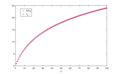
Figure 9: Comparison of $\mathbb{E}[X_{n}]$, the expected time that the $n^{\mathrm{th}}$ block arrives, with $z_{n}$, the time at which the expected number of blocks arrived is $n$, for $\lambda(t)=e^{at}$ with $a=0.1$.

The results above for $\mathbb{E}[X_{n}]$ and $z_{n}$ are for single segments only, we have not included the dependency caused by changes in the difficulty. Now we investigate the behaviour of the times at which difficulty changes occur. While these are random variables, we approximate them with a deterministic version $y_{n}$: the times such that the average number of arrivals since the last difficulty change is 2,016, that is, for $n\geq 1$

$$2016 =\int_{y_{n-1}}^{y_{n}}\lambda(t)\,dt=\int_{y_{n-1}}^{y_{n}}\frac{H(t)}{2^{32}D(t)}\,dt=\int_{y_{n-1}}^{y_{n}}\frac{H(t)}{2^{32}D_{n}}\,dt.$$ (28)

We fix $H(t)$ and the starting difficulty $D_{1}=d_{1}\geq 1$, and determine each subsequent difficulty change as in the random version, but instead of using the random arrival times to adjust the difficulty, we use the deterministic approximation. The difficulty on $(y_{n},y_{n+1})$ is then given by

$$d_{n+1}=d_{n}\frac{\texttt{2 weeks}}{y_{n}-y_{n-1}}\,,$$ (29)

for $n\geq 1$.

Let $\delta_{n}=y_{n}-y_{n-1}$, and thus $y_{n}=y_{0}+\sum_{i=1}^{n}\delta_{i}$ and use fortnights (2 weeks) as our unit of time. We have for $n\geq 2$

$$d_{n}=d_{n-1}/\delta_{n-1}=d_{1}/\prod_{i=1}^{n-1}\delta_{i}\,.$$ (30)

If we assume an exponential hash rate $\widehat{H}(t)=e^{at+b}$ with $a>0$ we can use Equation (28) to find a recursion for the sequence $(\delta_{n})_{n=2}^{\infty}$

$$2016 =\int_{y_{n-1}}^{y_{n}}\frac{e^{at+b}}{d_{n}}\,dt=\frac{e^{b}}{ad_{n}}(e^{ay_{n}}-e^{ay_{n-1}})$$

$$=\frac{e^{ay_{n-1}+b}}{ad_{n}}(e^{a\delta_{n}}-1)$$ (31)

so that

$$e^{a\delta_{n}}-1 =\frac{ad_{1}/\prod_{i=1}^{n-1}\delta_{i}}{\exp(ay_{0}+b+a\sum_{i=1}^{n-1}\delta_{i})}$$

$$=\frac{ad_{1}/\prod_{i=1}^{n-2}\delta_{i}}{b\exp(ay_{0}+a\sum_{i=1}^{n-2}\delta_{i})}\cdot\frac{1}{e^{a\delta_{n-1}}\delta_{n-1}}$$

$$=\frac{e^{a\delta_{n-1}}-1}{e^{a\delta_{n-1}}\delta_{n-1}}.$$ (32)

Thus

$$\delta_{n}=\frac{1}{a}\log\left(\frac{e^{a\delta_{n-1}}-1}{e^{a\delta_{n-1}}\delta_{n-1}}+1\right).$$ (33)

Consider the sequence $A_{n}=(e^{a\delta_{n}}-1)_{n=1}^{\infty}$. Equation (32) shows that

$$A_{n}=A_{n-1}/{(e^{a\delta_{n-1}}\delta_{n-1})}.$$

Thus if $\delta^{*}=\lim_{n\rightarrow\infty}\delta_{n}$ exists, then $\lim_{n\rightarrow\infty}A_{n}=0$ or $\delta^{*}$ satisfies

$$e^{a\delta^{*}}\delta^{*}=1$$ (34)

which is consistent with Equation (8). However, $\lim_{n\rightarrow\infty}A_{n}=0$ implies that $\lim_{n\rightarrow\infty}\delta_{n}=0$, but $\lim_{\delta_{n-1}\rightarrow 0}A_{n-1}/(e^{a\delta_{n-1}}\delta_{n-1})=a$, a contradiction. Thus we have shown that if $\delta^{*}$ exists then it must satisfy Equation (34).

An alternative means of expressing Equation (34) is

$$\delta^{*}=\frac{1}{a}W(a)$$ (35)

where $W(\cdot)$ is the Lambert-W function [19, 20], defined so that $x=W(xe^{x})$. We now show that $\delta^{*}=\lim_{n\rightarrow\infty}\delta_{n}$ exists.

Consider the function $f(\delta)=\frac{1}{a}\log\left(\frac{e^{a\delta}-1}{e^{a\delta}\delta}+1\right)$, defined so that $\delta_{n+1}=f(\delta_{n})$. We will show that $f^{(n)}(\delta_{1})$ tends to a limit regardless of $\delta_{1}>0$. Taking the derivative,

$$f^{\prime}(\delta)=\frac{a\delta-e^{a\delta}+1}{a\delta((\delta+1)e^{a\delta}-1)}.$$ (36)

Then $f^{\prime}(\delta)$ is increasing from $\frac{-a}{2(1+a)}$ to $0$ as $\delta$ goes from $0$ to $\infty$, thus $-\frac{1}{2}<\frac{-a}{2(1+a)}<f^{\prime}(\delta)<0$ and consequently $f(\delta)$ is a contraction for $\delta\in(0,\infty)$. Therefore, by the Banach fixed point theorem, we know that $\delta^{*}=\lim_{n\rightarrow\infty}f^{(n)}(\delta_{1})=\lim_{n\rightarrow\infty}\delta_{n}$ exists and satisfies $f(\delta)=\delta$, and thus it is given by the unique solution of Equation (34).

Equation (34) has the following interpretation: if a steady state is to occur, the ratio $e^{a\delta}$ by which the hash rate increases over the period of a segment should be equal to the corresponding increase in the difficulty. This increase in the difficulty is given by the ratio $1/\delta$ of a fortnight to the actual time taken for the segment. In the case of this deterministic approximation, the system settles down to a steady state regardless of initial conditions.

We can use this deterministic approximation for the times and magnitudes of the difficulty changes as the basis of a nonhomogeneous Poisson process model over a timescale spanning successive segments. In such a model the difficulty changes are now deterministic, and so there is no dependency on disjoint intervals to prevent the block arrival process from being Poisson.

IV-E Including the block propagation delay in the block arrival model

Our model does not yet account for the time taken for a newly discovered block to propagate through the network and have its transactions validated at each node. While this affects the times that blocks arrive at a measurement node, it does not directly change the timestamps of the blocks. However, it does affect the block inter-arrival process as a whole. When a new block is mined, it has to propagate through the Bitcoin network to each other miner and be validated before that miner can start mining on it. Block propagation delay thus has an effect on the rate at which mining is performed. We will use a simple method for modelling the delay: we treat it as an effective reduction in the block arrival rate for a period after a block is mined. We provide two options:

1. The simplest option is to model it as a constant delay to every miner, and ignore the hash power contribution from the miner of the block (who sees no propagation delay). Thus we would take any of our previous models and add a period after each block arrival when no blocks could be mined.

2. The second option is to assume that the block does not arrive at all nodes at once, but gradually reaches a greater and greater proportion of the miners (or more importantly, a greater and greater proportion of the mining power). If we assume that the rate at which miners receive the block is proportional to the number of miners who have not yet received it, we obtain an exponential model for the delay. In this case, if the most recent block arrived at time $s$, then the effective global hash rate at time $t$ is $(1-e^{c(t-s)})H(t)$.

   This approach is consistent with the way in which [10] and [21] refer to propagation delay: they quantify it in each case by saying “on average a block will arrive at 90% of nodes within $x$ seconds”, where $x$ is 26 and 79 respectively.

We examine the consequences of this approach in more detail in the following section. In the simulation experiments presented in Section VI we will only consider option 2.

V Summary of the block arrival models

There are several aspects of the block arrival models proposed in this paper. We provide a summary of these differing options here before using a simulation to evaluate them in the following section.

1. The hash rate function can be modelled 1(a) parametrically, or 1(b) empirically.

   We will use $\widehat{H}(t)=e^{at+b}$ as the parametric hash rate model and $H^{W}_{144}(t)$ as the empirical hash rate model.

2. The difficulty adjustments are 2(a) deterministic, or 2(b) random.

   The real blockchain has random difficulty adjustments, in that they occur every 2,016 blocks of a random process, and their magnitude depends on the time those blocks took to arrive. However, we saw in Section IV-D2 that given the hash rate function, we can find the expected times and magnitudes of these difficulty adjustments, and use those instead to approximate the block arrival process.

3. The 3(a) absence, or 3(b) presence of block propagation delay and how the delay is modelled (Section IV-E).

Regardless of whether the global hash rate $H(t)$ is modelled empirically or parametrically, for each of the block arrival models in this paper the hash rate is determined before the random process $X_{i}(t)$ is sampled.

• For the models 22(a) with deterministic difficulty adjustments, the difficulty is adjusted at deterministic time instants $y_{n}$ which do not correspond to the random instants of block arrivals, and the block arrival rate $\lambda(t)$ is independent of the block arrivals in the preceeding segments. If there is no delay 33(a), then on each interval the model is a nonhomogeneous Poisson process.

• For the models 22(b) with random difficulty adjustment, the difficulty is adjusted at random time instants corresponding to the end of each 2,016 block segment using Equation (1). If there is no delay 33(a), then on each segment the process is a nonhomogeneous Poisson process with rate given by $\lambda(t)={H(t)}/{D_{i}}$. Since the block arrival rate $\lambda(t)$ depends upon the first and last arrivals in the previous segment, the process is not a Poisson process over a timescale spanning successive segments.

• If propagation delay is present 33(b), then the block arrival process is not a nonhomogeneous Poisson process even on a single segment.

In the following section we will compare simulations of these models to the timestamp data from the Bitcoin blockchain.

VI Simulations and comparison with blockchain data

VI-A Exponential hash rate, random difficulty changes, no block propagation delay

We approximate the hash rate $H(t)$ with an exponential function $\widehat{H}(t)=e^{at+b}$. The block arrival rate is $\lambda(t)={\widehat{H}(t)}/{(2^{32}D(t))}$ as in Equation (22), where the difficulty $D(t)$ changes every 2,016 blocks as in Equation (1). We developed two independent implementations of the simulation model. The outputs of the two simulators agreed closely. The average results for each interval are given in Table II. While the estimate $H^{W}_{144}(t)$ of the real hash rate fluctuates around the exponential approximation $\widehat{H}(t)$ (see Figure 5), the average block inter-arrival time in each interval closely matches the observed mean with the exception of interval 5 from March 2013 to October 2014.

We can also see (Figure 6) that the mean inter-arrival time from the simulations closely matches the mean predicted by the steady state approximation given in Equation (35) regardless of the value of the exponential coefficient $a$.

VI-B Modifications for simulating the block propagation delay

When simulating our models with propagation delay, we must take into account the effect of that delay on the apparent hash rate, and re-estimate the hash rate taking the (hypothesised) value of the delay into account. Let the estimate of the underlying hash rate (the number of hashes being checked per second, valid or otherwise) be $\widehat{H}(t)$ and the effective hash rate be $\widetilde{H}(t)=(1-e^{c(t-s)})\widehat{H}(t)$.

If we assume an exponential hash rate function $\widehat{H}(t)=e^{at+b}$ with random difficulty changes, then for the period between $X_{i}$ and $X_{i+1}$, the number of effective hashes checked is

$$\int_{X_{i}}^{X_{i+1}}\widetilde{H}(t)\,dt$$ (37)

$$= \int_{X_{i}}^{X_{i+1}}(1-e^{c(t-X_{i})})\widehat{H}(t)\,dt$$

$$= \int_{X_{i}}^{X_{i+1}}(1-e^{c(t-X_{i})})e^{at+b}\,dt$$

$$= e^{aX_{i}+b}\int_{0}^{X_{i+1}-X_{i}}(e^{at}-e^{(a+c)t})\,dt$$

$$= \widehat{H}(X_{i})\bigg{[}\frac{e^{at}}{a}-\frac{e^{(c+a)t}}{c+a}\bigg{]}_{0}^{X_{i+1}-X_{i}}$$

$$= \widehat{H}(X_{i})\bigg{(}\frac{e^{a(X_{i+1}-X_{i})}-1}{a}-\frac{e^{(a+c)(X_{i+1}-X_{i})}-1}{a+c}\bigg{)}.$$

If we approximate the $X_{i}$ by their measured values we can invert this relationship to obtain a corrected estimate for $H(t)$ in the exponential case. The process is similar if we use an empirical hash rate function.

If we want to simulate a model with deterministic difficulty changes, we must employ a slightly more complicated version of this process to estimate the times at which difficulty changes occur. This is because the arrival rate is not constant over the interval. The adjusted arrival rate $\widetilde{\lambda}(t)$ is given by

$$\widetilde{\lambda}(t)=\frac{\lambda(t)}{1+{\lambda(t)}/{c}}=\frac{1}{{1}/{\lambda(t)}+{1}/{c}}$$ (38)

where $\lambda(t)={H(t)}/{(2^{32}D(t))}$. Thus we must solve for $y_{i+1}=X_{2016(i+1)}$ in

$$\int_{y_{i}}^{y_{i+1}}\widetilde{\lambda}(t)dt$$ (39)

iteratively for each $i$ to get the expected difficulty change times $y_{i+1}$.

interval	2	3	4	5	6
Observed mean	491.8	459.1	586.9	503.2	575.7
Simulated mean	491.6	462.6	589.2	493.8	576.9
Observed s.d.	503.3	477.6	578.1	494.7	567.3
Simulated s.d.	493.7	465.6	589.7	494.7	578.0

Table II: Simulation experiments using an exponential hash rate function, random difficulty changes and zero block propagation delay: the mean and standard deviation of the block inter-arrival times in seconds for each interval.

VI-C Discrepancies between the observed and simulated values of the standard deviation of the inter-arrival times

Table II shows that the average block inter-arrival time of the observed data and the simulation using the random difficulty change model match reasonably well in all the intervals except interval 5 from March 2013 to October 2014, but the standard deviation of the simulated data often does not match well with the observed data. There are two possible reasons for this.

• The first reason is the error in the block arrival times. Let $X_{i}$ be the $i^{\mathrm{th}}$ block timestamp, let $W_{i}$ be the time that block $i$ was actually created, and let $\epsilon_{i}$ be the error in timestamp $i$, so that

  $$X_{i}=W_{i}+\epsilon_{i}.$$ (40)

  Then if the $\epsilon_{i}$ are independent and identically distributed with variance $\mathrm{Var}(\epsilon)$, we would have the variance of the timestamp inter-arrival times

  $$\mathrm{Var}(X_{i}-X_{i-1})=\mathrm{Var}(W_{i+1}-W_{i})+2\,\mathrm{Var}(\epsilon).$$ (41)

  Thus the timestamp errors would increase the variance. This conclusion is true even if the variance of the errors is not constant over time. The data cleaning (Section II-C) reduces this effect but does not eliminate or reverse it. If we examine Table II we see that in some intervals the standard deviation of the timestamp inter-arrival data is lower than that predicted by simulation, so it cannot be entirely a result of errors in the block timestamps.

• The second explanation as to why the timestamp inter-arrival time data has a different variance to that predicted by the models is the effect of the block propagation delay. Propagation delay reduces the effective global hash rate because some time is used mining blocks which will not be included in the long-term blockchain. However, the difficulty adjusts to compensate for the loss of hash rate. Small values of the delay (relative to the mean inter-arrival time) therefore have little effect on the overall mean, but do change the shape of the inter-arrival time distribution. This reduces the probability that blocks have very low inter-arrival times, so it might be expected that it reduces the variance of the inter-arrival times, and in fact this is what happens.

To test the effect of block propagation delay on the distribution of inter-arrival times we simulate delay as in option 2 in Section IV-E, where the effective global hash rate is $(1-e^{c(t-s)})H(t)$ where the most recent block was mined at time $s$. We plot the effects on the mean and standard deviation of the simulated inter-arrival times $X_{i}-X_{i-1}$ for a range of values of $c$ in Figures 10 through 14. Rather than displaying the actual values of $c$ on the horizontal axis we instead show the median delay because it is more intuitive.

Figures 10 through 14 show the mean of 100 simulations for each set of parameters. The 95% confidence intervals are too small to be seen on the graph. The solid lines in each plot are the simulation results. The horizontal dashed lines are the values calculated from the observed LR resampled timestamp data for each interval. For the simulated model to fit the real data, the solid lines must intersect the dashed lines of the same colour. Ideally the simulated mean and standard deviation will intersect the observed mean and standard deviation for the same value of the delay, that is, the intersections will line up vertically. The dotted line is the mean block arrival interval $\delta^{*}=W(a)/a$ predicted by the steady state deterministic approximation given in Equation (34). The average block arrival interval $\delta^{\ast}$ varies with $c$ because $a$ is the slope of the line fitted to the logarithm of the estimated hash rate, and the estimate of the hash rate depends on $c$ (see Section VI-B).

VI-D Exponential hash rate, random difficulty changes with delay

Figures 10 through 14, subfigures (a) shows what happens when we use an exponential function and random difficulty changes to approximate the hash rate. In all intervals except interval 5 the observed mean is well approximated by using a reasonable value of the block propagation delay. This model is also consistent with the observed values of the standard deviation in the more recent intervals 4, 5 and 6, typically for a median block propagation delay of around 7 seconds. However, the standard deviation of the observed inter-arrival data in intervals 2 and 3 is much higher than that the standard deviations of the simulated model for all values of the block propagation delay. This could be due to the highly variable hash rate in intervals 2 and 3 being poorly modelled by the exponential approximation. To address this we can use a more highly fitted, empirical hash rate function.

VI-E Empirical hash rate with delay

Figures 10 through 14, subfigure (c) shows what happens when we use the empirical function $H^{W}_{144}(t)$ to approximate the hash rate, with random difficulty changes. We consider this to be the most detailed and accurate model of those presented here. In each interval it is clear that this model is generally successful at matching the observed block inter-arrival time statistics by our criterion defined above: the median delay value at which the simulated lines intersect the measured (“real”) values of the parameters is usually around 10 seconds (it is lower for interval 3). Note that in most cases the true delay is likely to be higher, due to the random errors in the timestamp data artificially increasing the measured standard deviation (the true dashed line would be lower, making the solid line intersect it at a higher difficulty value).

When comparing the values of median delay inferred here to those generated in the measurement studies [10] and [21], the delay values mentioned in this paper are for miner-to-miner propagation delay, rather than general node-to-node propagation delays. Miners have a strong economic incentive to be better connected to the Bitcoin network than a general Bitcoin node, therefore in the present day they would be expected to have a lower median delay.

VI-F Deterministic difficulty changes

Figures 10 through 14, subfigures (b) and (d) show the the results for simulations of models with deterministic difficulty changes. Subfigure (b) corresponds to the model with an exponential hash rate, and subfigure (d) corresponds to the model with an empirical hash rate. In each case we can see the simulated mean and standard deviation values are close to those of the corresponding models with random difficulty changes for low values of propagation delay, but as the propagation delay increases the deterministic approximation loses accuracy. For high values of the propagation delay, the deterministic models uniformly have lower means and standard deviations of inter-arrival times.

(a) Exponential hash rate function, random difficulty changes

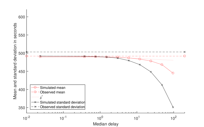
(b) Exponential hash rate function, deterministic difficulty changes

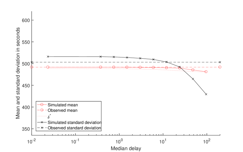
(c) Empirical hash rate function, random difficulty changes

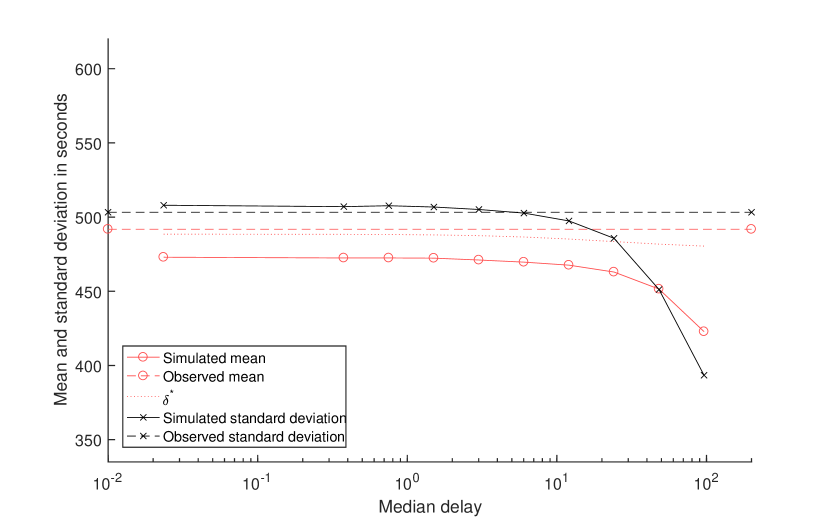
(d) Empirical hash rate function, deterministic difficulty changes

Figure 10: Interval 2. Simulating the effect of block propagation delay (seconds) on the statistics of the inter-arrival time distributions. The dashed lines indicate the values measured in the blockchain. The dotted line is the value of the mean inter-arrival time predicted in Equation (35) by substituting in the value of $a$ estimated from the blockchain timestamp data and converting from mean segment time in fortnights to mean inter-arrival time in seconds.

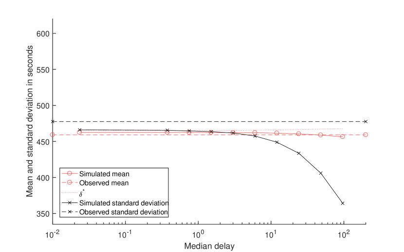
(a) Exponential hash rate function, random difficulty changes

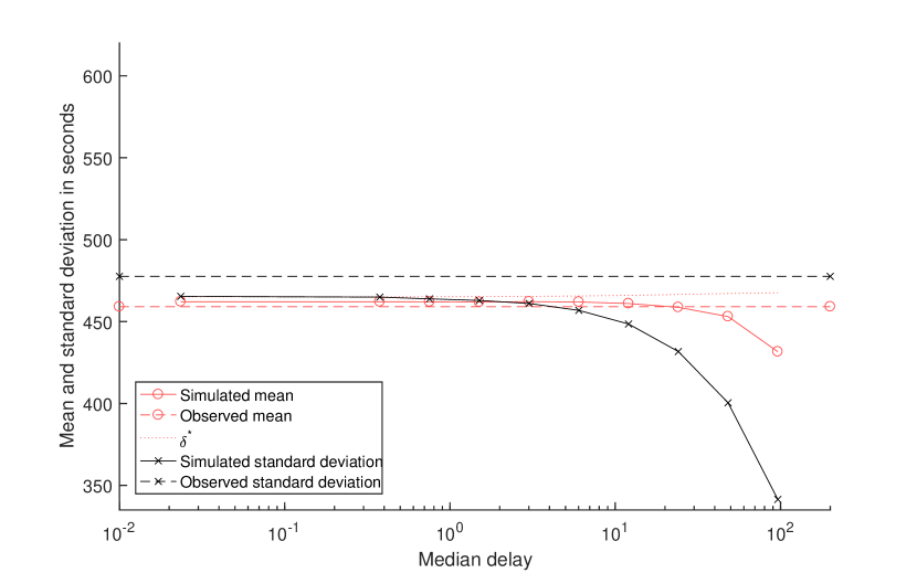
(b) Exponential hash rate function, deterministic difficulty changes

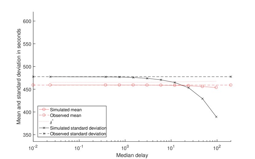
(c) Empirical hash rate function, random difficulty changes

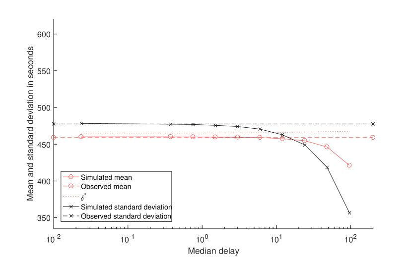
(d) Empirical hash rate function, deterministic difficulty changes

Figure 11: Interval 3. Simulating the effect of block propagation delay (seconds) on the statistics of the inter-arrival time distributions. The dashed lines indicate the values measured in the blockchain. The dotted line is the value of the mean predicted in Equation (35) by substituting in the value of $a$ estimated from the blockchain timestamp data.

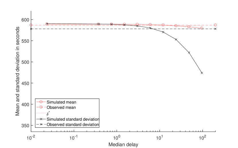
(a) Exponential hash rate function, random difficulty changes

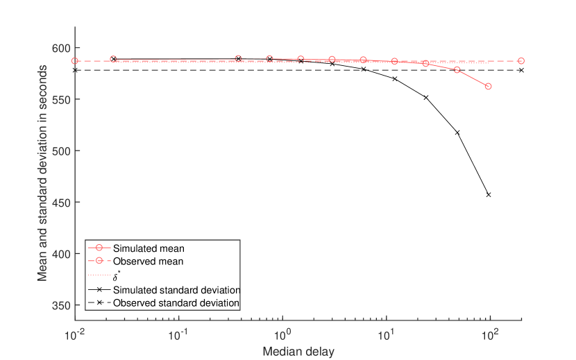
(b) Exponential hash rate function, deterministic difficulty changes

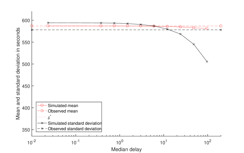
(c) Empirical hash rate function, random difficulty changes

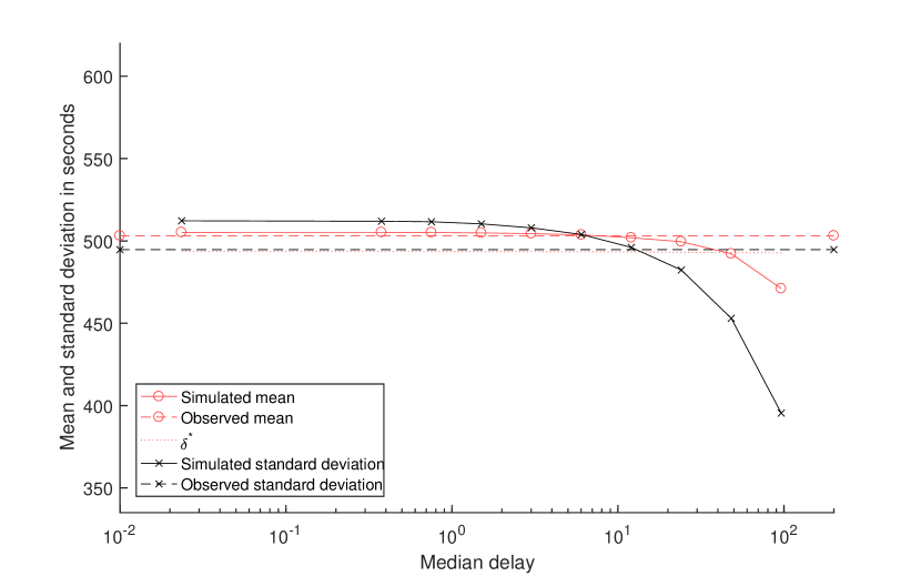
(d) Empirical hash rate function, deterministic difficulty changes

Figure 12: Interval 4. Simulating the effect of block propagation delay (seconds) on the statistics of the inter-arrival time distributions. The dashed lines indicate the values measured in the blockchain. The dotted line is the value of the mean predicted in Equation (35) by substituting in the value of $a$ estimated from the blockchain timestamp data.

(a) Exponential hash rate function, random difficulty changes

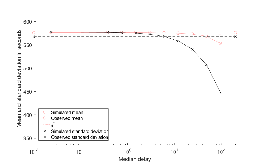
(b) Exponential hash rate function, deterministic difficulty changes

(c) Empirical hash rate function, random difficulty changes

(d) Empirical hash rate function, deterministic difficulty changes

Figure 13: Interval 5. Simulating the effect of block propagation delay (seconds) on the statistics of the inter-arrival time distributions. The dashed lines indicate the values measured in the blockchain. The dotted line is the value of the mean predicted in Equation (35) by substituting in the value of $a$ estimated from the blockchain timestamp data.

(a) Exponential hash rate function, random difficulty changes

(b) Exponential hash rate function, deterministic difficulty changes

(c) Empirical hash rate function, random difficulty changes

(d) Empirical hash rate function, deterministic difficulty changes

Figure 14: Interval 6. Simulating the effect of block propagation delay (seconds) on the statistics of the inter-arrival time distributions. The dashed lines indicate the values measured in the blockchain. The dotted line is the value of the mean predicted in Equation (35) by substituting in the value of $a$ estimated from the blockchain timestamp data.

VI-G A summary of model performance and recommendations

In this subsection we consider which models and in what circumstances they should be used. We use the notation outlined in Section V.

1. The most accurate and successful model is 11(b) 22(b) 33(b) – empirical hash rate, random difficulty changes and propagation delay included. We would recommend this model whenever it is possible to closely estimate the hash rate and accurate results are required. This is also the most complicated model.

2. The next most accurate model is 11(a) 22(b) 33(b) – this is the same as above, but with an exponential hash rate. This model is accurate whenever the growth in the hash rate is expected to be to be approximately exponential. This would include the present day and could include a short period into the future, so this model might be reasonable for forecasting.

3. The simplest model that we recommend is 11(a) 22(a) 33(a) – exponential hash rate, deterministic difficulty changes and no propagation delay. This model is a nonhomogeneous Poisson process where the hash rate function is periodic. The rate increases exponentially over each segment then instantaneously returns to its initial value at the end of each segment. This model provides a reasonable approximation to the block arrival process while still remaining analytically tractable.

For the latter two options, if the long term block arrival rate is all that is required it can be calculated with Equation (10) or (35).

VII Conclusion

In this paper we have presented a suite of models for the point process of block mining epochs in the Bitcoin blockchain, and tested it with both simulation and data available from the blockchain itself. The main challenges in doing this are:

1. the unknown global hash rate that drives the rate of block discovery; and

2. the historically known, but random, mining difficulty value.

Furthermore, the data on the times at which blocks arrive is comprehensive, but not completely reliable. We postulate a point process model in which the block arrival process behaves as a nonhomogeneous Poisson process on times between difficulty changes with rate proportional to the ratio of the hash rate to the difficulty, but which is dependent on itself when difficulty changes are taken into account. For a given global hash rate, the times at which the difficulty changes (and hence the block arrival rate changes) are determined by the sample-path of the process. self-correcting. Nevertheless, the global hash rate is consistently rapidly increasing and the difficulty feedback mechanism is sufficiently delayed so that the rate of block arrivals has been around 11.5% greater than the base rate of 6 per hour. This means that overall, the transaction throughput and the total miner income from bounties are higher than in the base case. Furthermore, the times when the block mining bounty is halved and the time when all bitcoins have been created will occur earlier than they would have if blocks were mined at a rate of six per hour.

In addition to giving a model for the block arrival process, we have derived the relationship between block arrival rates and the rate of exponential increase of the hash rate. We have also provided a practical approximation that exhibits limiting behaviour independent of initial conditions and perturbations of the block arrival process, and verify this approximation with simulation and measurements from the blockchain.

Appendix A Proof of Equation (25)

For $1\leq n\leq 2016$ and $a>0$

$$\mathbb{E}[X_{n}|X_{0}=0] =\int_{0}^{\infty}xf_{X_{n}|X_{0}=0}(x)\,dx$$

$$=\int_{0}^{\infty}xe^{ax}e^{-\frac{1}{a}(e^{ax}-e^{0a})}(\frac{1}{a}(e^{ax}-e^{0a}))^{n-1}\frac{1}{(n-1)!}\,dx$$

$$=\int_{0}^{\infty}xe^{ax}e^{-\frac{1}{a}(e^{ax}-1)}(\frac{1}{a}(e^{ax}-1))^{n-1}\frac{1}{(n-1)!}\,dx.$$

Setting $g(t)=e^{at}$ and $h(t)=\mathrm{exp}(-(e^{at}-1)/a)$ and for $n=1,2,\ldots$ let

$$I_{n}(x)=\int_{\infty}^{x}g(t)(g(t)-1)^{n-1}h(t)\,dt.$$ (42)

Integration by parts gives

$$\mathbb{E}[X_{n}|X_{0}=0] =\frac{1}{(n-1)!a^{n-1}}\int_{0}^{\infty}xg(x)(g(x)-1)^{n-1}h(x)\,dx$$

$$=\frac{1}{(n-1)!a^{n-1}}\left(\Big{[}xI_{n}(x)\Big{]}_{0}^{\infty}-\int_{0}^{\infty}I_{n}(x)\,dx\right).$$ (43)

We proceed by finding an expression for $I_{n}(x)$. Note first that $\frac{d}{dx}h(x)=-g(x)h(x)$. Once again applying integration by parts gives (for $n\geq 2$):

$$I_{n}(x) =\int_{\infty}^{x}gh(g-1)^{n-1}\,dt$$

$$=-h(g-1)^{n-1}-\int_{\infty}^{x}ag(g-1)^{n-2}(n-1)(-h)\,dt$$

$$=-h(g-1)^{n-1}+a(n-1)I_{n-1}(x).$$

Combining this with $I_{1}(x)=\int_{\infty}^{x}gh\,dt=-h(x)$ and setting the constant of integration to 0 we get (for $n\geq 1$):

$$I_{n}(x)=-h\sum_{i=0}^{n-1}\frac{(n-1)!}{i!}a^{n-1-i}(g-1)^{i}.$$ (44)

Similarly

$$\int_{\infty}^{x}g^{n}h\,dt=-h(x)\sum_{i=0}^{n-1}\frac{(n-1)!}{i!}a^{n-1-i}g(x)^{i}.$$ (45)

Thus

$$\int_{0}^{\infty}I_{n}(x)\,dx =\int_{0}^{\infty}-h\sum_{i=0}^{n-1}\frac{(n-1)!}{i!}a^{n-1-i}(g-1)^{i}\,dx$$

$$=\int_{0}^{\infty}-h\sum_{i=0}^{n-1}\frac{(n-1)!}{i!}a^{n-1-i}\sum_{j=0}^{i}\binom{i}{j}g^{j}(-1)^{i-j}\,dx$$

$$=\sum_{i=0}^{n-1}(n-1)!a^{n-1-i}\sum_{j=0}^{i}\frac{(-1)^{i+j+1}}{j!(i-j)!}\int_{0}^{\infty}g^{j}h\,dx$$

$$=\sum_{i=0}^{n-1}(n-1)!a^{n-1-i}\left(\frac{(-1)^{i+1}}{i!}\int_{0}^{\infty}h\,dx+\sum_{j=1}^{i}\frac{(-1)^{i+j}}{j!(i-j)!}\bigg{[}h\sum_{k=0}^{j-1}\frac{(j-1)!}{k!}a^{j-1-k}g^{k}\bigg{]}_{0}^{\infty}\right)$$

$$=\sum_{i=0}^{n-1}(n-1)!a^{n-1-i}\left(\frac{(-1)^{i}}{i!a}e^{1/a}\mathrm{Ei}(-\frac{1}{a})+\sum_{j=1}^{i}\frac{(-1)^{i+j+1}}{j(i-j)!}\sum_{k=0}^{j-1}\frac{a^{j-1-k}}{k!}\right)\,,$$ (46)

where the last line uses

$$\int_{0}^{\infty}h\,dx = \int_{0}^{\infty}\mathrm{exp}(-(e^{ax}-1)/a)\,dx$$

$$= \frac{e^{1/a}}{a}\int_{1/a}^{\infty}\frac{e^{-u}}{u}\,dx=-\frac{e^{1/a}}{a}\mathrm{Ei}(-\frac{1}{a}).$$

Now we can evaluate (43)

$$\mathbb{E}[X_{n}|X_{0}=0]=\frac{1}{(n-1)!a^{n-1}}\left([xI_{n}(x)]_{0}^{\infty}-\int_{0}^{\infty}I_{n}(x)\,dx\right)\,,$$ (47)

which, via equations (44) and (46), becomes

$$\mathbb{E}[ X_{n}|X_{0}=0]$$ (48)

$$= \frac{1}{(n-1)!a^{n-1}}\times\left(0-\sum_{i=0}^{n-1}(n-1)!a^{n-1-i}\left(\frac{(-1)^{i}}{i!a}e^{1/a}\mathrm{Ei}(-\frac{1}{a})+\sum_{j=1}^{i}\frac{(-1)^{i-j+1}}{j(i-j)!}\sum_{k=0}^{j-1}\frac{a^{j-1-k}}{k!}\right)\right)$$

$$= \sum_{i=0}^{n-1}a^{-i}\left(\frac{(-1)^{i+1}}{i!a}e^{1/a}\mathrm{Ei}(-\frac{1}{a})+\sum_{j=1}^{i}\frac{(-1)^{i+j}}{j(i-j)!}\sum_{k=0}^{j-1}\frac{a^{j-1-k}}{k!}\right)$$

$$= \sum_{i=0}^{n-1}(-a)^{-i}\left(\frac{-e^{1/a}}{i!a}\mathrm{Ei}(-\frac{1}{a})+\sum_{j=1}^{i}\frac{(-a)^{j}}{j(i-j)!}\sum_{k=0}^{j-1}\frac{a^{-1-k}}{k!}\right)$$

$$= \sum_{i=0}^{n-1}(-a)^{-i-1}\left(\frac{e^{1/a}}{i!}\mathrm{Ei}(-\frac{1}{a})-\sum_{j=1}^{i}\frac{(-a)^{j}}{j(i-j)!}\sum_{k=0}^{j-1}\frac{a^{-k}}{k!}\right).$$ (49)

References

- [1] S. Nakamoto, Bitcoin: A peer-to-peer electronic cash system (2008).
-
[2]
T. Dodd,
University
of Melbourne first in Australia to use blockchain for student records,
Australian Financial Review April 30, 2017.
URL http://www.afr.com/leadership/university-of-melbourne-first-in-australia-to-use-blockchain-for-student-records-20170427-gvubid - [3] M. Rosenfeld, Analysis of hashrate-based double spending, arXiv preprint arXiv:1402.2009.
- [4] J. Göbel, H. P. Keeler, A. E. Krzesinski, P. G. Taylor, Bitcoin blockchain dynamics: The selfish-mine strategy in the presence of propagation delay, Performance Evaluation 104 (2016) 23–41.
- [5] M. Rosenfeld, Analysis of bitcoin pooled mining reward systems, arXiv preprint arXiv:1112.4980.
- [6] Y. Lewenberg, Y. Bachrach, Y. Sompolinsky, A. Zohar, J. S. Rosenschein, Bitcoin mining pools: A cooperative game theoretic analysis, in: Proceedings of the 2015 International Conference on Autonomous Agents and Multiagent Systems, International Foundation for Autonomous Agents and Multiagent Systems, 2015, pp. 919–927.
- [7] I. Eyal, E. G. Sirer, Majority is not enough: Bitcoin mining is vulnerable, in: International Conference on Financial Cryptography and Data Security, Springer, 2014, pp. 436–454.
- [8] A. Sapirshtein, Y. Sompolinsky, A. Zohar, Optimal selfish mining strategies in bitcoin, in: International Conference on Financial Cryptography and Data Security, Springer, 2016, pp. 515–532.
- [9] S. Solat, M. Potop-Butucaru, Zeroblock: Preventing selfish mining in Bitcoin, arXiv preprint arXiv:1605.02435.
- [10] C. Decker, R. Wattenhofer, Information propagation in the bitcoin network, in: 2013 IEEE Thirteenth International Conference on Peer-to-Peer Computing (P2P), IEEE, 2013, pp. 1–10.
- [11] A. Miller, J. J. LaViola Jr, Anonymous byzantine consensus from moderately-hard puzzles: A model for bitcoin, Available on line: http://nakamotoinstitute. org/research/anonymous-byzantine-consensus.
- [12] R. Bowden, Intersection of longest increasing subsequences, https://github.com/rhysbowden/LIS (Nov. 2017).
- [13] V. A. Epanechnikov, Non-parametric estimation of a multivariate probability density, Theory of Probability & Its Applications 14 (1) (1969) 153–158.
- [14] D. J. Daley, D. Vere-Jones, An introduction to the theory of point processes, vol. 1, Springer, New York, 2003.
- [15] L. Brown, N. Gans, A. Mandelbaum, A. Sakov, H. Shen, S. Zeltyn, L. Zhao, Statistical analysis of a telephone call center: A queueing-science perspective, Journal of the American Statistical Association 100 (469) (2005) 36–50.
- [16] S.-H. Kim, W. Whitt, Choosing arrival process models for service systems: Tests of a nonhomogeneous Poisson process, Naval Research Logistics (NRL) 61 (1) (2014) 66–90.
- [17] J. F. C. Kingman, Poisson processes, Vol. 3, Oxford University Press, 1992.
- [18] H. W. Lilliefors, On the Kolmogorov-Smirnov test for the exponential distribution with mean unknown, Journal of the American Statistical Association 64 (325) (1969) 387–389.
- [19] R. M. Corless, G. H. Gonnet, D. E. Hare, D. J. Jeffrey, D. E. Knuth, On the Lambert W function, Advances in Computational mathematics 5 (1) (1996) 329–359.
- [20] J. H. Lambert, Observationes variae in mathesin puram, Acta Helveticae 3 (1) (1758) 128–168.
- [21] K. Croman, C. Decker, I. Eyal, A. E. Gencer, A. Juels, A. Kosba, A. Miller, P. Saxena, E. Shi, E. G. Sirer, D. Song, R. Wattenhofer, On scaling decentralized blockchains, in: International Conference on Financial Cryptography and Data Security, Springer, 2016, pp. 106–125.