The Hubble Space Telescope UV Legacy Survey of Galactic Globular Clusters. XIII. ACS/WFC Parallel-Field Catalogues††thanks: Based on observations with the NASA/ESA Hubble Space Telescope, obtained at the Space Telescope Science Institute, which is operated by AURA, Inc., under NASA contract NAS 526555.
Abstract
As part of the Hubble Space Telescope UV Legacy Survey of Galactic Globular Clusters, 110 parallel fields were observed with the Wide Field Channel of the Advanced Camera for Surveys, in the outskirts of 48 globular clusters, plus the open cluster NGC 6791. Totalling about square degrees of observed sky, this is the largest homogeneous Hubble Space Telescope photometric survey of Galalctic globular clusters outskirts to date. In particular, two distinct pointings have been obtained for each target on average, all centred at about arcmin from the cluster centre, thus covering a mean area of about for each globular cluster. For each field, at least one exposure in both F475W and F814W filters was collected. In this work, we publicly release the astrometric and photometric catalogues and the astrometrised atlases for each of these fields.
keywords:
globular clusters: general – Hertzsprung-Russel and colour-magnitude diagrams; catalogues and atlases.1 Introduction
For almost three decades, the Milky Way Globular Clusters (GCs) have been the target of large CCD photometric surveys aimed at sampling their stellar populations in a homogeneous way (Rosenberg et al. 2000a, Rosenberg et al. 2000b, Piotto et al. 2002, Sarajedini et al. 2007) using both space- and ground-based instruments. The growing sample of data, and the advent of increasingly sophisticated data-analysis techniques, have clearly demonstrated that GCs host distinct stellar populations with different chemical abundances. High-precision photometric measurements have revealed that the colour-magnitude diagrams (CMDs) show distinct sequences in various evolutionary stages (see e.g. Anderson 1997, Lee et al. 1999, Pancino et al. 2000, Bedin et al. 2004, Piotto et al. 2007, Milone et al. 2008, Bellini et al. 2010). These findings are also supported by spectroscopical evidence that the stellar populations of these systems are not as simple as thought (see e.g. Marino et al. 2008, Yong & Grundahl 2008, Kraft 1994, Carretta et al. 2009a, Carretta et al. 2009b, Gratton et al. 2004, Gratton et al. 2012).
The Hubble Space Telescope UV Legacy Survey of Galactic Globular Clusters (GO-13297; PI:Piotto) has been specifically designed to further investigate this phenomenon and it now appears likely that all Galactic GCs host multiple stellar populations (Piotto et al. 2015 – hereafter Paper I, Milone et al. 2017 – hereafter Paper IX). In the context of this survey, parallel Advanced Camera for Surveys (ACS) observations have been obtained. While the main observations were taken using a combination of UV and optical filters of the Wide Field Camera 3 (WFC3), the lack of filters bluer than F435W dictated the use of the F475W and F814W filters of the Wide Field Channel of the ACS (ACS/WFC) in the parallel observations. The large colour baseline provided by this filter combination guarantees sensitivity to helium abundance differences, while being largely insensitive to star-to-star variations in light-element abundances (Sbordone et al. 2011, Cassisi et al. 2017).
One of the main objectives for which these observations were planned is to investigate how different stellar populations formed in GCs. Strong observational constraints come from the analysis of the radial distribution of each stellar population (D’Ercole et al. 2008; Bellini et al. 2009, Vesperini et al. 2013). As an example, Simioni et al. (2016) complemented WFC3 data of the central regions of NGC 2808 with ACS parallel observations and found evidence of different radial trends associated with distinct stellar populations hosted by the cluster. Thus, clusters with large helium variations among their stellar populations are the preferred target of investigation with the current data-sample. Other interesting targets, albeit extensively studied, are those defined as Type-II clusters in Paper IX, which displays multiple sub-giant branches in optical CMDs.
We stress the fact that this is the first homogeneous HST photometric survey of the outskirts of Galactic GCs. The observations presented here represent a first epoch for future studies aimed at systematical measurements of absolute, relative and internal proper motions of stars in these regions. Archival HST observations matching a sub-sample of the observed fields exist, and proper motions will be published separately. In the imaged stellar fields, the stellar density is not as high as in the central regions. As a consequence, crowding is not a serious issue for these data. That makes them particularly suitable to be used as input catalogue for future spectroscopic surveys.
The present catalogues can be used to perform several interesting analyses. For example, dynamical interactions between stars in GCs is at the origin of the mass segregation phenomenon. A precise estimate of its effects is fundamental for the derivation of a global mass function for a GC (Vesperini & Heggie 1997, Paust et al. 2010, Sollima & Baumgardt 2017). The measurement of the fraction of binaries is also fundamental for this kind of analysis and could provide useful constraints for dynamical models (Milone et al., 2012). We note, also, that in some cases white dwarf cooling sequences are visible in the obtained CMDs. Finally, it is interesting to note that due to the presence of many extra-galactic objects in the observed field, other studies could benefit from these observations.
In this work, we present the first photometric catalogues from the ACS/WFC parallel observations of the GO-13297 program. All data have been reduced in a homogeneous manner, making these catalogues particularly suitable for inter-comparison. The article is organised as follows: in Section 2 the data are presented along with some information about the observing strategy, together with a detailed description of the data reduction. The extracted CMDs are presented in Section 3. Details on the selection of well measured stars are given in Section 4. In Section 5 the catalogues and the released electronic material are described in detail. Finally, in Section 6, after a summary, we briefly discuss some of the main scientific questions we will address with these catalogues in subsequent papers.
2 Observations and Data Reduction
we show right ascension and declination of each distinct parallel field, referred to the centre of ACS/WFC. We also report the number of orbits, Telescope orientation (V3 PA) for each orbit and exposure time in each filter. # CLUSTER ORBITS FIELD RA (J2000) DEC (J2000) EPOCH EXP. TIME EXP. TIME [PA (deg)] F475W (s) F814W (s) 01 NGC1261 5 F1 [92] 03:12:49.68 -55:17:25.2 31/08/13 770 694 F2 [138] 03:12:16.96 -55:19:29.6 11/09/13 745 669 F3 [182] 03:11:44.35 -55:17:39.3 08/11/13 766 690 F4 [225] 03:11:30.53 -55:13:17.9 07/12/13 745 669 F5 [48] 03:13:01.92 -55:12:51.4 29/06/14 829 753 02 NGC1851 7 F1 [195] 05:13:37.57 -40:06:44.0 27/12/10 2x40;2x1277;1237 6x488;1x40 F2 [164] 05:13:51.57 -40:08:55.8 11/11/10 2x40;2x1277;2x1237 8x488;2x40 03 NGC2298 4 F1 [185] 06:48:36.04 -36:05:08.7 18/12/13 2x785 2x683 F2 [273] 06:48:35.14 -35:55:40.7 07/03/14 885 816 15/03/15 887 815 04 NGC3201 2 F1 [25] 10:18:12.19 -46:21:47.1 13/09/13 685 612 F2 [115] 10:17:54.00 -46:30:51.0 01/01/14 689 616 05 NGC4590 2 F1 [112] 12:39:42.64 -26:50:34.9 21/12/13 627 554 F2 [202] 12:39:01.10 -26:47:48.5 30/03/14 627 554 06 NGC4833 4 F1 [113] 13:00:10.12 -70:58:29.4 17/01/14 2x840 2x771 F2 [202] 12:58:20.68 -70:55:42.6 09/04/14 2x806 2x730 07 NGC5024 6 F1 [31] 13:13:21.59 +18:12:01.1 24/03/14 4x725;2x723 3x370 F2 [120] 13:13:03.82 18:03:52.0 08/12/13 4x775;2x774 3x375 08 NGC5053 5 F1 [352] 13:16:42.03 +17:47:28.7 01/04/14 740 664 F2 [37] 13:16;53.97 +17:43:15.0 16/03/14 740 664 F3 [80] 13:16;50.28 +17:38:33.1 23/01/14 790 714 F4 [125] 13:16;33.21 +17:35:39.5 05/12/13 790 714 F5 [308] 13:16;21.88 +17:48:25.0 16/05/14 765 689 09 NGC5286 2 F1 [73] 13:47:07.09 -51:25:00.2 14/12/13 728 655 F2 [162] 13:46:11.09 -51:28:46.7 15/03/14 603 559 10 NGC5466 4 F1 [112] 14:05:41.08 +28:26:12.1 05/01/14 834;835 763;765 F2 [21] 14:05:54.29 +28:35:18.1 29/03/14 2x776 2x700 11 NGC5897 4 F1 [112] 15:17:37.48 -21:06:27.5 12/02/14 830;833 2x761 F2 [202] 15:16:58.75 -21:03:44.3 13/05/14 779;781 710;709 12 NGC5904 2 F1 [323] 15:18:34.23 02:11:38.3 17/05/14 620 559 F2 [52] 15:19:00.34 02:04:36.4 08/04/14 621 559 13 NGC5927 3 F1 [100] 15:28:28.73 -50:45:30.4 01/02/14 603 559 F2 [189] 15:27:28.26 -50:44:48.7 19/05/14 603 559 27/05/15 603 559 14 NGC5986 3 F1 [92] 15:46:28.87 -37:51:38.6 27/01/14 676 603 F2 [180] 15:45:40.83 -37:52:21.9 17/05/14 603 559 10/05/15 603 559 15 NGC6093 5 F1 [255] 16:16:35.04 -22:55:45.9 09/06/12 5x760;5x845 5x539 16 NGC6101 5 F1 [147] 16:25:36.08 -72:18:35.2 04/04/14 762 686 F2 [190] 16:24:40.57 -72:16:07.7 25/05/14 762 686 F3 [235] 16:24:23.48 -72:11:18.6 29/06/14 800 724 F4 [282] 16:24:58.26 -72:06:50.7 14/08/13 851 775 F5 [101] 16:26:39.71 -72:17:19.9 28/02/14 800 724 17 NGC6121 2 F1 [272] 16:23:12.57 -26:27:02.1 06/07/14 739 666 F2 [98] 16:23:55.64 -26:36:33.4 17/02/15 666 593 18 NGC6144 2 F1 [83] 16:27:39.42 -26:05:00.9 28/02/14 679 606 F2 [174] 16:26:57.33 -26:07:05.2 27/05/14 679 606 19 NGC6171 4 F1 [342] 16:32:41.94 -12:56:56.1 31/05/14 830;833 2x761 F2 [72] 16:32:42.20 -12:57:07.5 25/03/14 800;802 731;730 20 NGC6218 2 F1 [276] 16:46:55.21 -01:52:03.7 16/08/13 721 648 F2 [6] 16:47:33.42 -01:52:07.7 27/05/14 645 572 21 NGC6254 2 F1 [276] 16:56:50.04 -04:01:10.1 16/08/13 721 648 F2 [7] 16:57:28.66 -04:01:19.2 27/05/14 644 571 22 NGC6304 2 F1 [184] 17:14:10.53 -29:32:35.1 07/06/14 624 559 F2 [274] 17:14:09.53 -29:23:04.8 26/08/13 731 658 23 NGC6341 2 F1 [230] 17:16:30.21 +43:08:03.0 22/10/13 638 565 F2 [319] 17:17:06.19 +43:14:56.0 03/08/14 750 677 24 NGC6352 2 F1 [161] 17:25:15.00 -48:31:41.7 27/05/14 637 564 F2 [251] 17:24:51.02 -48:22:52.5 13/08/13 731 658 Continued on Tab. 2
Tables 2 and 2 report the log of ACS/WFC observations used to construct the catalogues. For each target, we indicate the total number of orbits assigned to each observed field separated by the different position angles (PAs) of the V3 axis of the HST focal plane. Typically, one F475W and one F814W image were taken each orbit, with a dither between the two dictated by primary WFC3 observing strategy. For each field, right ascension and declination of the centre of ACS/WFC are provided along with exposure time in each filter.
![[Uncaptioned image]](/html/1801.07445/assets/x1.png)
![[Uncaptioned image]](/html/1801.07445/assets/x2.png)
![[Uncaptioned image]](/html/1801.07445/assets/x3.png)
The physical position of ACS/WFC detectors in the focal plane of HST is such that its projected field of view (FoV) in the sky is located at a distance of about arcminutes from the centre of the WFC3 FoV. Depending on the number of orbits allocated to each GC, from to a maximum of non-overlapping fields were observed. This is because, in order to secure a good handling of charge-transfer-efficiency (CTE) systematic errors, primary WFC3 observations were taken by applying a different telescope rotation at each orbit (Paper I, Section 4). For the majority of clusters, which were allocated orbits, a rotation of about was performed between the first and second orbit; for clusters observed for more than orbits, a minimum difference of between the V3 PA of each orbit was required. Five distinct pointings were obtained for 3 clusters, namely NGC 1261, NGC 5053 and NGC 6101. Three distinct fields were obtained for 4 clusters: NGC 6652, NGC 6717, NGC 6723 and NGC 7089. For the other clusters, only 2 pointings were planned. M80 is an exception and was not observed as part of the Program GO-13297. For it, we make use of archival HST data from GO-12311. When possible, ACS parallel observations targeted pre-existing HST observations.
Figures 2 and 2 – 2 display all HST observations that sample the sky area in the vicinity of those covered in this survey. Three cameras onboard HST were considered in order to enhance the probability of an overlap between observations: Wide Field and Planetary Camera 2 (WFPC2), ACS and WFC3 (both UVIS and IR channels). Taking 2 images per orbit, one in F475W and one in F814W filters, the typical exposure times for both filters are of the order of .
All exposures have been corrected for CTE effects using the method described in Anderson & Bedin (2010). Photometric measurements of stellar objects in each field have been performed using a suite of fortran programs based on img2xym (Anderson & King, 2006) and kitchen_sync presented in Anderson et al. (2008). The spatial variation of the PSF has been taken into account adopting a grid of model PSFs distributed along each image. However focus changes/breathing of the telescope, imperfect guiding, residual noise related to CTE can produce image-to-image variations of the PSF. To mitigate these sources of systematic errors, we derived a set of spatially varying perturbations of the PSF models for each calibrated, non-drizzled (flc) image. Adopting the procedure presented in Bellini et al. (2013), each image is divided into a grid with a number of cells changing from to . In each cell, a subset of well measured stars is used to locally adjust the PSF models to the stellar profiles. Using an updated version of Anderson & King (2006) software, in combination with the newly created PSF models, we extracted raw catalogues of stellar positions and magnitudes in each image. We choose the grid refinement (between to ) that produces the best results, inspecting the distribution of the quality of fit parameters as a function of magnitude, and taking into account the number of reference stars used to tailor the PSF perturbations in each cell.
Each exposure related to the same field has been subsequently referred to a common reference frame. Since we are mainly interested in the faint, red part of the cluster CMDs, we used the F814W images to construct the reference frames. Catalogues are finally produced using a version of the software presented in Anderson et al. (2008), specifically tuned for this project. In particular, the kitchen_sync routine has been modified in order to work properly with only one image per filter. In addition, the method presented in Gilliland (2004) was applied in order to provide reliable photometry also for saturated stars.
The raw, instrumental magnitudes have been zero-pointed into ACS/WFC Vega-mag photometric system following the prescriptions of Bedin et al. (2005). The zero-points and aperture corrections from arcseconds to infinity of Bohlin (2016) have been used.
Especially in the present case, the photometric calibration plays a critical role, and we put strong efforts to precisely evaluate zero-point differences between various observations. Crowding is not a serious problem in the outer cluster regions and high-precision photometric measurements are relatively easy to obtain. But field-to-field zero-point variations must be accounted for to have the external fields of the same cluster on the same photometric scale. The main source of this photometric offsets between catalogues of distinct fields, is related to PSF modelling. The PSF model by construction is normalized to a surface flux of unity within a radius of ACS/WFC pixels ( arcsecond). Only the inner -pixel region of sources was used to fit to the PSF model in order to minimize the contaminating impact of nearby neighbors, but any mismatch between the adopted PSF model and the pixels beyond the small square fitting aperture would result in a slight zeropoint shift. The fact that we perturb the library PSFs (above) minimizes this even further. However, the best way to regularize the photometry is empirically: following Bedin et al. (2005) and Anderson et al. (2008), we measured aperture corrections inside this aperture using the calibrated and drizzled (drc) images as reference.
| # | CLUSTER | FIELD | ||
|---|---|---|---|---|
| mag | mag | |||
| 01 | NGC1261 | 1 | ||
| 2 | ||||
| 3 | ||||
| 4 | ||||
| 5 | ||||
| 02 | NGC1851 | 1+2 | ||
| 03 | NGC2298 | 1 | ||
| 2 | ||||
| 04 | NGC3201 | 1 | ||
| 2 | ||||
| 05 | NGC4590 | 1 | ||
| 2 | ||||
| 06 | NGC4833 | 1 | ||
| 2 | ||||
| 07 | NGC5024 | 1 | ||
| 2 | ||||
| 08 | NGC5053 | 1 | ||
| 2 | ||||
| 3 | ||||
| 4 | ||||
| 5 | ||||
| 09 | NGC5286 | 1 | ||
| 2 | ||||
| 10 | NGC5466 | 1 | ||
| 2 | ||||
| 11 | NGC5897 | 1 | ||
| 2 | ||||
| 12 | NGC5904 | 1 | ||
| 2 | ||||
| 13 | NGC5927 | 1 | ||
| 2 | ||||
| 14 | NGC5986 | 1 | ||
| 2 | ||||
| 15 | NGC6093 | 1 | ||
| 16 | NGC6101 | 1 | ||
| 2 | ||||
| 3 | ||||
| 4 | ||||
| 5 | ||||
| 17 | NGC6121 | 1 | ||
| 2 | ||||
| 18 | NGC6144 | 1 | ||
| 2 | ||||
| 19 | NGC6171 | 1 | ||
| 2 | ||||
| 20 | NGC6218 | 1 | ||
| 2 | ||||
| 21 | NGC6254 | 1 | ||
| 2 | ||||
| 22 | NGC6304 | 1 | ||
| 2 | ||||
| 23 | NGC6341 | 1 | ||
| 2 | ||||
| 24 | NGC6352 | 1 | ||
| 2 |
Continued on Tab. 2
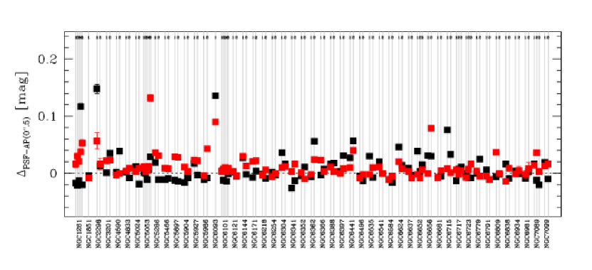
These corrections were sufficient to properly take into account the majority of the photometric biases in our catalogues. The obtained values of the aperture correction for an aperture of arcseconds are listed in Tables 2 and 2. We maintain the same nomenclature as in Bedin et al. (2005). The aperture correction values, along with their associated uncertainties are also reported in Figure 2. Black dots are referred to F814W observations, red dots to F475W ones. It can be noted that for the majority of cases corrections are small: typically smaller than magnitudes, but in the most severe cases, they can reach values as high as mag.
continued on Table 2
Astrometrised, stacked images of each observed field have also been produced for both filters with a pixel sampling. These have been created, for each field, combining all overlapping flc images using the same coordinate transformations that define the common reference frames.
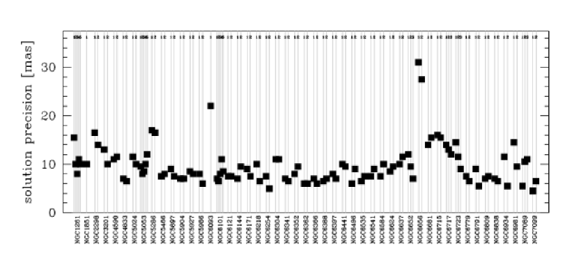
Astrometric solutions have been independently derived using the Gaia DR1 catalogue as a reference (Gaia Collaboration et al., 2016). As a consequence, positions are given for Equinox J2000 at epoch 2015. Table 2 reports the precision reached by the new astrometric solution in the fifth column, which is the root mean square error of the offset between Gaia positions and those derived, for the same stars, in our astrometrised stacked images. The measured average value is pixel, or milliarcseconds. These values are also visualised in Figure 3.
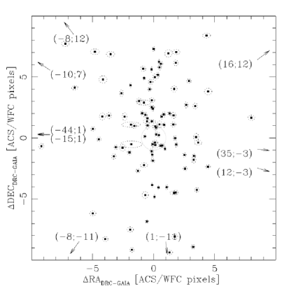
For completeness, we also measure the astrometric precision of the original astrometric solution of drc images. The position offset between common sources in the Gaia DR1 catalogue and the drc images is used to define this quantity. Offset values are referred to RA and DEC distances in image pixels and are reported in columns six and seven of Table 2. The associated errors corresponds to the measured standard deviations of each sample. A visual representation is also given in Figure 4. It can be noted that, in general, offsets are lower than ACS/WFC pixels ( arcseconds), and, in many cases, below pixel, with some notable exceptions.
3 The Colour-Magnitude Diagrams and trichromatic stacked images
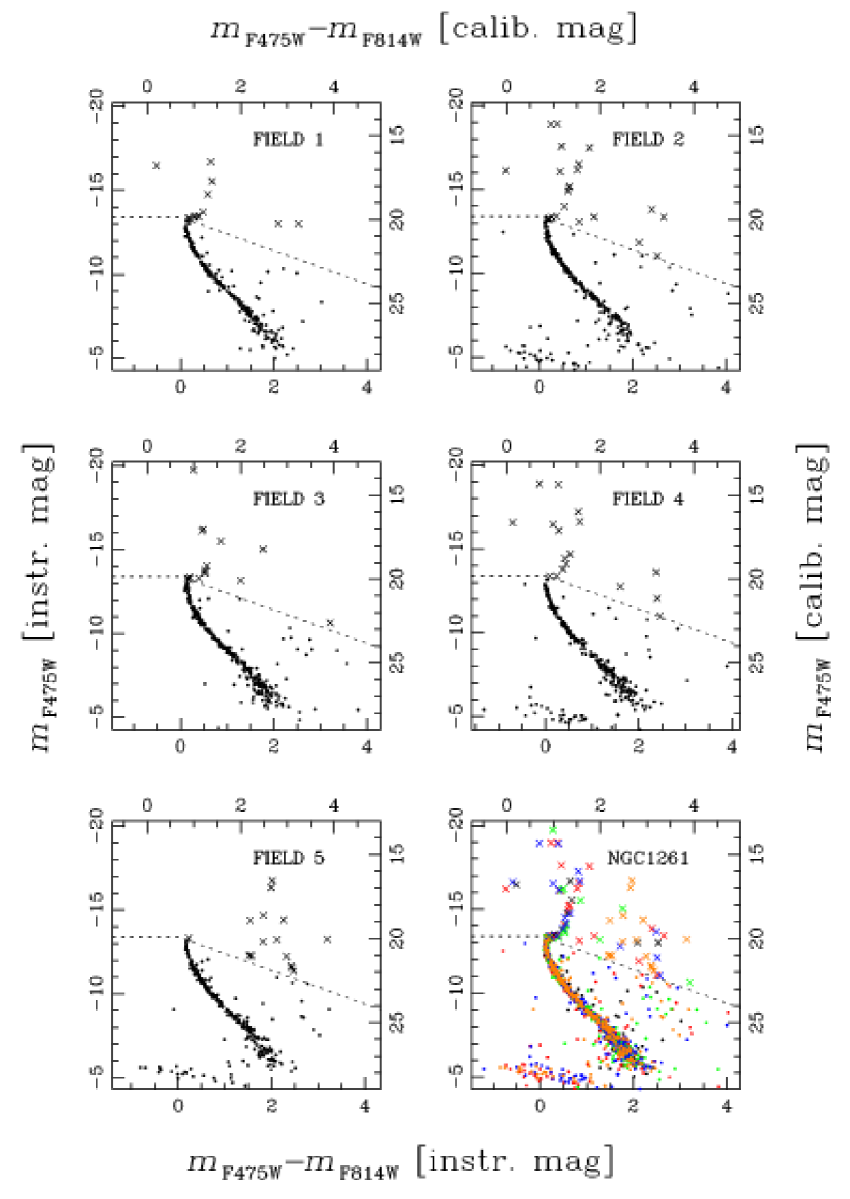
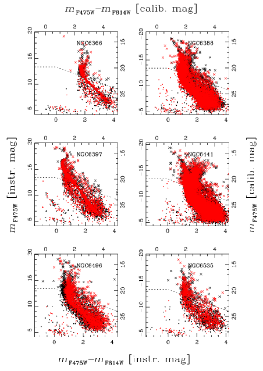
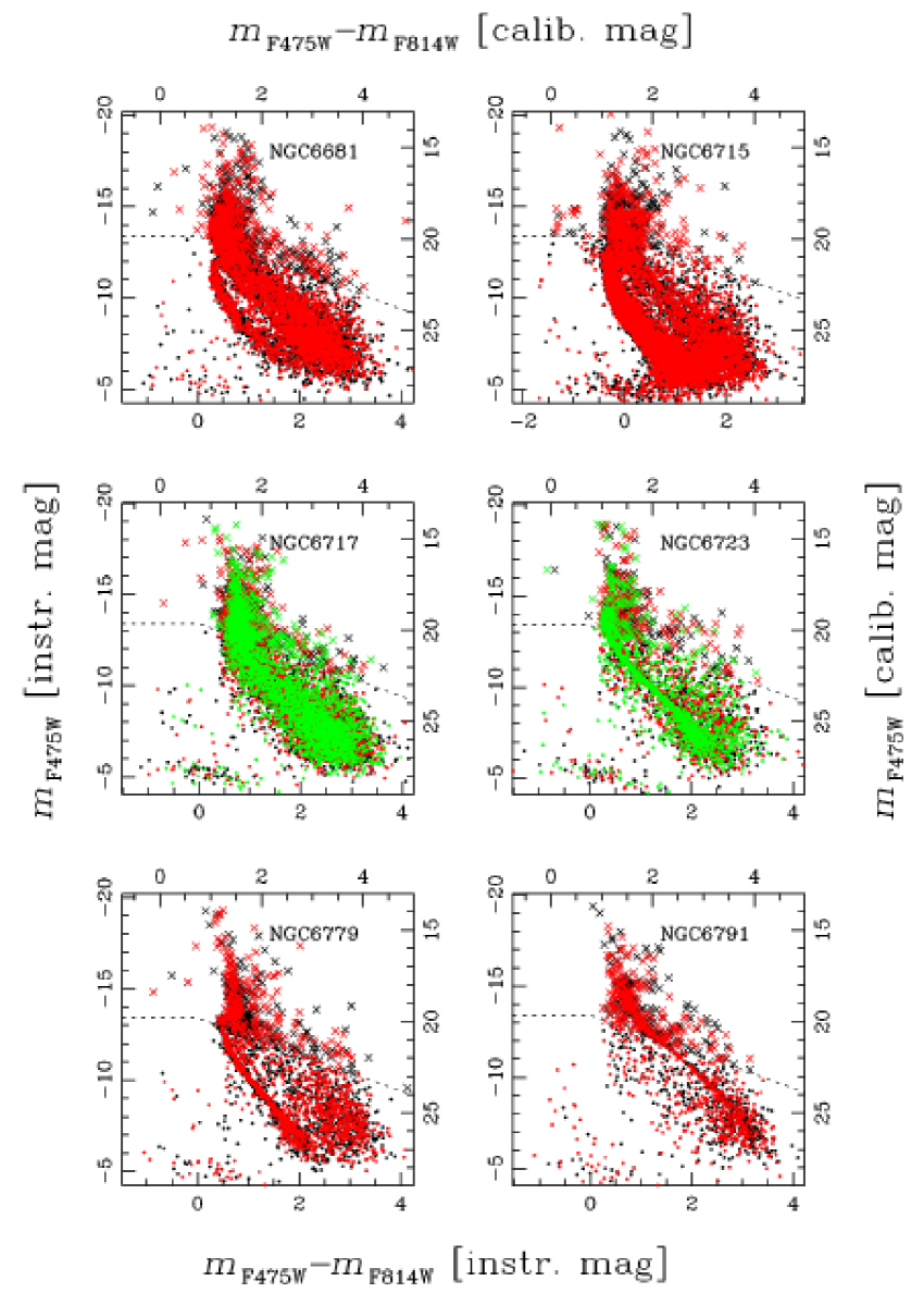
In Figure 5 we report the CMDs obtained for all 5 fields of NGC 1261. Magnitudes are given both in the instrumental and Vega-mag photometric systems. Dashed lines represent the saturation limit, black dots represent unsaturated stars, saturated stars are represented with crosses. The five CMDs are all merged in the bottom-right panel, where a different colour have been assigned to each different field. In this case, the instrumental magnitude scale, along with saturation level (dashed line), refer only to Field 1.
The final CMDs for all other targets are presented in Figures 16 - 23. The presented CMDs have been obtained by selecting only high-quality stars, according to quality parameters presented in Anderson et al. (2008). In Section 4 we describe the adopted selection procedure. It is important to mention here that, since in the majority of the cases only one image per filter has been taken, artifact rejection is not an easy task. In order to include faint sources, we have chosen not to limit in flux our raw catalogues. We nonetheless restricted the detections only to those sources observed in at least one F814W and one F475W image simultaneously, with positions in the common reference frame consistent within pixels.
No rejection of foreground/background contamination has been performed, nor any correction for differential reddening. The homogeneity of the data guarantees very similar results in every case. Nonetheless, it is out of the scope of the present work to characterize in detail the obtained results, which require taking into consideration several issues. For example, the number density of cluster members present in the observed fields depends on the properties of each GC: in some cases, especially for bulge clusters, or those that appear projected in this dense Galactic region, it is difficult to identify the cluster sequence. We recall that another interesting application of the present data is the study of the stellar populations, external to the clusters, that contaminate the observed fields. In particular, for at least 6 GCs, namely NGC 6624, NGC 6637, NGC 6652, NGC 6681, NGC 6715 and NGC 6809, traces of the Sagittarius Stream are visible in the obtained CMDs (Siegel et al., 2011).
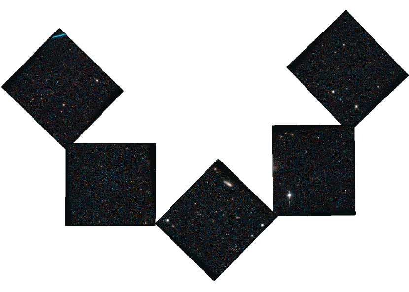
As an additional tool to explore and characterize observations, we have created colour images of each observed field, combining the astrometrised stacked images: an example is shown in Figure 6. The F814W stacked images have been associated with red channel while the F475W images are associated to the blue channel. The images associated to the green channel have been obtained as a result of a 3:1 weighted mean of F475W and F814W counts respectively.
4 Selection of well-measured stars
This section describes the procedure adopted to reject spurious or poorly measured sources in the catalogues and to obtain a sample of bona-fide stellar sources. In this example we refer to the catalogue associated to Field 1 of NGC 6121 (M4). The V3 PA is 272 degrees and, for this field, 2 images were collected, one in F814W, and the other in F475W (666 and 739 seconds respectively).
For the selection, we have adopted a procedure similar to that described in Milone et al. (2012), defining limits in both q and o (quality) parameters. In addition, we also made use of the RADXS parameter (Bedin et al. 2008, Bedin et al. 2009, Bedin et al. 2010).
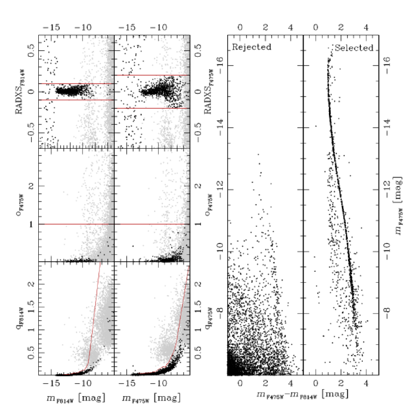
As shown in the lower left panels of Figure 7, the q parameter displays a characteristic trend with magnitude. This parameter is defined as the absolute value of the subtraction between the PSF model and the spatial distribution of light of a particular detection in the image, inside the fitting radius. For a perfectly modeled source, the q parameter assumes value .
The o parameter quantifies the amount of light that falls on the aperture used for PSF fitting, due to neighboring sources (Anderson et al., 2008). Unlike the q parameter, it does not shows a clear trend with magnitude (middle-left panels of Figure 7), for this reason we have used a fixed limit (Milone et al., 2012).
Finally, the RADXS parameter is related to the spatial extent of the sources, and it is used to distinguish between point sources and extended sources. It is defined as the flux in excess of that predicted from the PSF fitting just outside the core of each source (Bedin et al., 2008). Positive values are expected for extended objects, while negative values indicate detections that are sharper than stellar. The introduction of this parameter in the selection process for the present case is particularly necessary: since only one image per filter is available for most cases, spurious detections due to cosmic rays are present in the catalogues. Moreover, these observations cover the external regions of GCs, where the stellar density is not as high as in the central regions. The observed fields are thus relatively populated by extra-galactic, non-stellar objects.
We started by taking a more stringent limit in position-consistency for each source. We selected only sources with an rms error in position less than pixel. We adopted fixed limits in the o and RADXS parameters for both filters simultaneously. Finally, we measured, for the sources that survived this first selection, the median trend in the plane defined by magnitude and q parameter values. In this way, we removed from the sample non-stellar and poorly-measured sources, while not a priori losing faint sources. Red lines in the left panels of Figure 7 represent the limits used for the case of Field 1 of NGC 6121 (M4). Black points represent sources that passed the selection process. The CMD corresponding to rejected sources (grey dots in the left panels) is shown in the second panel from the right.
The resulting CMD is shown in the right panel of Figure 7. Note how the cleaning process allows the clear detection of the white-dwarf cooling sequence. Saturated stars have been excluded from the selection procedure, but their fluxes have been recovered using the procedure described in Gilliland (2004).
5 Released Electronic Material
#id      ra(2015)     dec(2015)     x         dx    y         dy    F814W  di    F475W  db     qi    qb    oi    ob    RADXSi  RADXSb  ni nb wi wb good
00000001 245.78962440  -26.47823845   549.416 0.353   688.174 0.224 28.832 9.900 27.078 9.900 1.620 0.760 1.526 0.115 -0.9900 -0.9157  1  1  1  1 0
00000002 245.78961100  -26.47812901   557.336 0.452   687.260 0.382 26.948 9.900 29.764 9.900 1.384 1.274 0.772 9.900  6.2647 -0.9900  1  1  1  1 0
00000003 245.78968050  -26.47823281   549.844 0.632   691.807 0.152 27.164 9.900 28.433 9.900 1.285 1.234 0.179 0.998 -0.9900 -0.9900  1  1  1  1 0
00000004 245.78969050  -26.47817087   554.332 0.391   692.424 0.136 27.335 9.900 30.545 9.900 1.229 1.715 1.014 2.384  0.9430 -0.9900  1  1  1  1 0
00000005 245.78969230  -26.47815496   555.485 0.426   692.537 0.076 27.109 9.900 29.691 9.900 1.189 1.274 0.404 9.900  2.2225 -0.9900  1  1  1  1 0
00000006 245.78973530  -26.47813294   557.094 0.032   695.317 0.263 28.421 9.900 28.038 9.900 1.204 1.009 3.708 0.336  5.6081 -0.9900  1  1  1  1 0
00000007 245.78971500  -26.47807749   561.102 0.068   693.975 0.088 27.108 9.900 28.184 9.900 1.187 0.948 0.787 0.228  1.0828 -0.9900  1  1  1  1 0
00000008 245.78970010  -26.47806742   561.826 0.001   693.008 0.354 26.711 9.900 30.436 9.900 1.154 1.722 0.354 2.059 -0.9900 -0.9900  1  1  1  1 0
00000009 245.78977530  -26.47818364   553.437 0.442   697.928 0.434 27.300 9.900 28.887 9.900 1.330 1.371 0.459 1.208 -0.7255  9.9900  1  1  1  1 0
00000010 245.79005820  -26.47833427   542.628 0.483   716.320 0.322 26.991 9.900 28.863 9.900 1.025 1.193 0.699 5.580  1.8430  1.1484  1  1  1  1 0
| Col. | Name | Explanation |
|---|---|---|
| 01 | id | ID number for each star |
| 02 | ra | Right Ascension for each star (in deg, epoch 2015) |
| 03 | dec | Declination for each star (in deg, epoch 2015) |
| 04 | x | x position of each star on the reference frame (in pixels) |
| 05 | dx | rms errors associated to x position (in pixels) |
| 06 | y | y position of each star on the reference frame (in pixels) |
| 07 | dy | rms errors associated to y position (in pixels) |
| 08 | F814W | F814W magnitude calibrated into Vegamag system |
| 09 | di | rms errors associated to F814W magnitude |
| 10 | F475W | F475W magnitude calibrated into Vegamag system |
| 11 | db | rms errors associated to F475W magnitude |
| 12 | qi | q parameter for F814W magnitudes |
| 13 | qb | q parameter for F475W magnitudes |
| 14 | oi | o parameter for F814W magnitudes |
| 15 | ob | o parameter for F475W magnitudes |
| 16 | RADXSi | RADXS parameter for F814W |
| 17 | RADXSb | RADXS parameter for F475W |
| 18 | ni | number of F814W images the source has been detected in |
| 19 | nb | number of F475W images the source has been detected in |
| 20 | wi | source of F814W photometry |
| 1: unsaturated in deep; 2: unsaturated in short; | ||
| 3: saturated in short; 4: saturated in deep; | ||
| 21 | wb | source of F475W photometry (same as wi) |
| 22 | good | the source has passed the selction process |
We release, for each ACS/WFC parallel field, the astrometric and photometric catalogues and trichromatic astrometrised stacked images. All the released material will be available for download at the website of the Exoplanets & Stellar Populations Group of the Università degli Studi di Padova111http://groups.dfa.unipd.it/ESPG/treasury.php.
Table 7 shows the first ten rows of the catalogue produced for Field 1 of NGC 6121. The content of each column is explained in detail in Table 8. The parameters wi and wb are the same as in Anderson et al. (2008). They are records that represent the level of saturation of each source in F814W and F475W images respectively. The last column includes the results of the selection of well-measured stars presented in Section 4.
Note that for many stars, we report a magnitude rms error of . This is because the routine empirically determines errors based on multiple observations in each filter. When there is only one observation per filter, the error is given a high default value.
6 Summary and Conclusions
In the context of the Hubble Space Telescope UV Legacy Survey Treasury program of Galactic Globular Clusters (GO-13297; PI: Piotto, Paper I), we are releasing the photometric catalogues relative to the ACS/WFC parallel observations. They represent the first HST photometric survey of external regions of Galactic GCs and consist of distinct stellar fields of targets: GCs and one open cluster, NGC 6791.
In the majority of cases, only two images per field were taken, one in F814W and one in F475W, centred at about arcminutes from cluster centre. Exposure times were selected in order to obtain reliable photometry of the main sequence of target GCs.
These observations complement the WFC3 observations of the central regions of the surveyed GCs, and represent valuable tools for different investigations as outlined in Paper I. These data represent a first epoch for future studies aimed at proper motions measurements in these regions. Even without proper motions, these catalogues are suitable to various interesting studies such as measurements of mass functions and binaries fractions in external regions of GCs. Furthermore, crowding is not an issue in these external cluster fields, as a result, this database could be also used as an input list for spectroscopic follow-up, for example for precise chemical tagging of cluster members.
Acknowledgements
We thank the anonymous referee for his careful revision that improved the quality of the present manuscript. M.S., A.A. and G.P. acknowledge support from the Spanish Ministry of Economy and Competitiveness (MINECO) under grant AYA2013-42781. M.S. and A.A. acknowledge support from the Instituto de Astrofísica de Canarias (IAC) under grant 309403. G.P. acknowledges partial support by the Università degli Studi di Padova Progetto di Ateneo CPDA141214 “Towards understanding complex star formation in Galactic globular clusters” and by INAF under the program PRIN-INAF2014. A.P.M. acknowledges support by the Australian Research Council through Discovery Early Carreer Researcher Award DE150101816 and by the ERC-StG 2016 716082 project ‘GALFOR’ funded by the European Research Council. This work has made use of data from the European Space Agency (ESA) mission Gaia (http://www.cosmos.esa.int/gaia), processed by the Gaia Data Processing and Analysis Consortium (DPAC, http://www.cosmos.esa.int/web/gaia/dpac/consortium). Funding for the DPAC has been provided by national institutions, in particular the institutions participating in the Gaia Multilateral Agreement.
References
- Anderson (1997) Anderson, A. J. 1997, Ph.D. Thesis, 1153
- Anderson & King (2006) Anderson, J., & King, I. R. 2006, Instrument Science Report ACS 2006-01, 34 pages,
- Anderson et al. (2008) Anderson, J., Sarajedini, A., Bedin, L. R., et al. 2008, AJ, 135, 2055
- Anderson & Bedin (2010) Anderson, J., & Bedin, L. R. 2010, PASP, 122, 1035
- Bedin et al. (2004) Bedin, L. R., Piotto, G., Anderson, J., et al. 2004, ApJ, 605, L125
- Bedin et al. (2005) Bedin, L. R., Cassisi, S., Castelli, F., et al. 2005, MNRAS, 357, 1038
- Bedin et al. (2008) Bedin, L. R., King, I. R., Anderson, J., et al. 2008, ApJ, 678, 1279-1291
- Bedin et al. (2009) Bedin, L. R., Salaris, M., Piotto, G., et al. 2009, ApJ, 697, 965
- Bedin et al. (2010) Bedin, L. R., Salaris, M., King, I. R., et al. 2010, ApJ, 708, L32
- Bellini et al. (2009) Bellini, A., Piotto, G., Bedin, L. R., et al. 2009, A&A, 507, 1393
- Bellini et al. (2010) Bellini, A., Bedin, L. R., Piotto, G., et al. 2010, AJ, 140, 631
- Bellini et al. (2013) Bellini, A., Anderson, J., Salaris, M., et al. 2013, ApJ, 769, L32
- Bohlin (2016) Bohlin, R. C. 2016, AJ, 152, 60
- Carretta et al. (2009a) Carretta, E., Bragaglia, A., Gratton, R. G., et al. 2009a, A&A, 505, 117
- Carretta et al. (2009b) Carretta, E., Bragaglia, A., Gratton, R., & Lucatello, S. 2009b, A&A, 505, 139
- Cassisi et al. (2017) Cassisi, S., Salaris, M., Pietrinferni, A., & Hyder, D. 2017, MNRAS, 464, 2341
- D’Ercole et al. (2008) D’Ercole, A., Vesperini, E., D’Antona, F., McMillan, S. L. W., & Recchi, S. 2008, MNRAS, 391, 825
- Gaia Collaboration et al. (2016) Gaia Collaboration, Brown, A. G. A., Vallenari, A., et al. 2016, A&A, 595, A2
- Gilliland (2004) Gilliland, R. L. 2004, Instrument Science Report ACS 2004-01, 18 pages,
- Gratton et al. (2004) Gratton, R., Sneden, C., & Carretta, E. 2004, ARA&A, 42, 385
- Gratton et al. (2012) Gratton, R. G., Carretta, E., & Bragaglia, A. 2012, A&ARv, 20, 50
- Harris 1996 (2010 edition) Harris, W. E. 1996, AJ, 112, 1487
- Kraft (1994) Kraft, R. P. 1994, PASP, 106, 553
- Lee et al. (1999) Lee, Y.-W., Joo, J.-M., Sohn, Y.-J., et al. 1999, Nature, 402, 55
- Marino et al. (2008) Marino, A. F., Villanova, S., Piotto, G., et al. 2008, A&A, 490, 625
- Milone et al. (2008) Milone, A. P., Bedin, L. R., Piotto, G., et al. 2008, ApJ, 673, 241-250
- Milone et al. (2012) Milone, A. P., Piotto, G., Bedin, L. R., et al. 2012, A&A, 540, A16
- Milone et al. (2017) Milone, A. P., Piotto, G., Renzini, A., et al. 2017, MNRAS, 464, 3636
- Pancino et al. (2000) Pancino, E., Ferraro, F. R., Bellazzini, M., Piotto, G., & Zoccali, M. 2000, ApJ, 534, L83
- Paust et al. (2010) Paust, N. E. Q., Reid, I. N., Piotto, G., et al. 2010, AJ, 139, 476
- Piotto et al. (2002) Piotto, G., King, I. R., Djorgovski, S. G., et al. 2002, A&A, 391, 945
- Piotto et al. (2007) Piotto, G., Bedin, L. R., Anderson, J., et al. 2007, ApJ, 661, L53
- Piotto et al. (2015) Piotto, G., Milone, A. P., Bedin, L. R., et al. 2015, AJ, 149, 91
- Rosenberg et al. (2000a) Rosenberg, A., Piotto, G., Saviane, I., & Aparicio, A. 2000 a, A&AS, 144, 5
- Rosenberg et al. (2000b) Rosenberg, A., Aparicio, A., Saviane, I., & Piotto, G. 2000 b, A&AS, 145, 451
- Sarajedini et al. (2007) Sarajedini, A., Bedin, L. R., Chaboyer, B., et al. 2007, AJ, 133, 1658
- Sbordone et al. (2011) Sbordone, L., Salaris, M., Weiss, A., & Cassisi, S. 2011, A&A, 534, A9
- Siegel et al. (2011) Siegel, M. H., Majewski, S. R., Law, D. R., et al. 2011, ApJ, 743, 20
- Simioni et al. (2016) Simioni, M., Milone, A. P., Bedin, L. R., et al. 2016, MNRAS,
- Sollima & Baumgardt (2017) Sollima, A., & Baumgardt, H. 2017, MNRAS, 471, 3668
- Vesperini & Heggie (1997) Vesperini, E., & Heggie, D. C. 1997, MNRAS, 289, 898
- Vesperini et al. (2013) Vesperini, E., McMillan, S. L. W., D’Antona, F., & D’Ercole, A. 2013, MNRAS, 429, 1913
- Yong & Grundahl (2008) Yong, D., & Grundahl, F. 2008, ApJ, 672, L29
Appendix A Extra material
In this section we complement Figures 2 and 5 with those referred to the rest of the sample. In particular, Figures 2, 2, 2, 2, 2, 2, 2 and 2 complement the sample of finding charts presented in Figure 2. Figures 16, 17, 18, 19, 20, 21, 22 and 23 are analogs to the lower-right panel of Figure 5.
![[Uncaptioned image]](/html/1801.07445/assets/x10.png)
![[Uncaptioned image]](/html/1801.07445/assets/x11.png)
![[Uncaptioned image]](/html/1801.07445/assets/x12.png)
![[Uncaptioned image]](/html/1801.07445/assets/x13.png)
![[Uncaptioned image]](/html/1801.07445/assets/x14.png)
![[Uncaptioned image]](/html/1801.07445/assets/x15.png)
![[Uncaptioned image]](/html/1801.07445/assets/x16.png)
![[Uncaptioned image]](/html/1801.07445/assets/x17.png)
![[Uncaptioned image]](/html/1801.07445/assets/x18.png)
![[Uncaptioned image]](/html/1801.07445/assets/x19.png)
![[Uncaptioned image]](/html/1801.07445/assets/x20.png)
![[Uncaptioned image]](/html/1801.07445/assets/x21.png)
![[Uncaptioned image]](/html/1801.07445/assets/x22.png)
![[Uncaptioned image]](/html/1801.07445/assets/x23.png)
![[Uncaptioned image]](/html/1801.07445/assets/x24.png)
![[Uncaptioned image]](/html/1801.07445/assets/x25.png)
![[Uncaptioned image]](/html/1801.07445/assets/x26.png)
![[Uncaptioned image]](/html/1801.07445/assets/x27.png)
![[Uncaptioned image]](/html/1801.07445/assets/x28.png)
![[Uncaptioned image]](/html/1801.07445/assets/x29.png)
![[Uncaptioned image]](/html/1801.07445/assets/x30.png)
![[Uncaptioned image]](/html/1801.07445/assets/x31.png)
![[Uncaptioned image]](/html/1801.07445/assets/x32.png)
![[Uncaptioned image]](/html/1801.07445/assets/x33.png)
![[Uncaptioned image]](/html/1801.07445/assets/x34.png)
![[Uncaptioned image]](/html/1801.07445/assets/x35.png)
![[Uncaptioned image]](/html/1801.07445/assets/x36.png)
![[Uncaptioned image]](/html/1801.07445/assets/x37.png)
![[Uncaptioned image]](/html/1801.07445/assets/x38.png)
![[Uncaptioned image]](/html/1801.07445/assets/x39.png)
![[Uncaptioned image]](/html/1801.07445/assets/x40.png)
![[Uncaptioned image]](/html/1801.07445/assets/x41.png)
![[Uncaptioned image]](/html/1801.07445/assets/x42.png)
![[Uncaptioned image]](/html/1801.07445/assets/x43.png)
![[Uncaptioned image]](/html/1801.07445/assets/x44.png)
![[Uncaptioned image]](/html/1801.07445/assets/x45.png)
![[Uncaptioned image]](/html/1801.07445/assets/x46.png)