INTERNAL VARIATIONS IN EMPIRICAL OXYGEN ABUNDANCES FOR GIANT H ii REGIONS
IN THE GALAXY NGC 2403

Abstract

This paper presents a spectroscopic investigation of 11 H ii regions in the nearby galaxy NGC 2403. The H ii regions are observed with a long-slit spectrograph mounted on the 2.16 m telescope at XingLong station of National Astronomical Observatories of China. For each of the H ii regions, spectra are extracted at different nebular radii along the slit-coverage. Oxygen abundances are empirically estimated from the strong-line indices $R23$, $N2O2$, $O3N2$, and $N2$ for each spectrophotometric unit, with both observation- and model-based calibrations adopted into the derivation. Radial profiles of these diversely estimated abundances are drawn for each nebula. In the results, the oxygen abundances separately estimated with the prescriptions on the basis of observations and models, albeit from the same spectral index, systematically deviate from each other; at the same time, the spectral indices $R23$ and $N2O2$ are distributed with flat profiles, whereas $N2$ and $O3N2$ exhibit apparent gradients with the nebular radius. Because our study naturally samples various ionization levels, which inherently decline at larger radii within individual H ii regions, the radial distributions indicate not only the robustness of $R23$ and $N2O2$ against ionization variations but also the sensitivity of $N2$ and $O3N2$ to the ionization parameter. The results in this paper provide observational corroboration of the theoretical prediction about the deviation in the empirical abundance diagnostics. Our future work is planned to investigate metal-poor H ii regions with measurable $T_{\mathrm{e}}$, in an attempt to recalibrate the strong-line indices and consequently disclose the cause of the discrepancies between the empirical oxygen abundances.

1. INTRODUCTION

H ii regions are gaseous nebulae ionized by high-energy radiation from young massive stars associated with star formation. Therefore, they are natural laboratories of star-forming activities and photoionization processes. The most striking characteristics of H ii regions are a wealth of hydrogen and metal emission lines in spectra. These spectral lines, coded by underlying physical properties, provide powerful insight into the nature of ionized nebulae and ionizing sources.

Oxygen abundance is a physical parameter usually derived from spectral lines at optical bands. Direct diagnostics of the oxygen abundance depend on estimates of electron temperature ($T_{\mathrm{e}}$) by measuring auroral lines such as $\hbox{[O\,{\sc iii}]}\lambda 4363$, $\hbox{[N\,{\sc ii}]}\lambda 5755$, and $\hbox{[S\,{\sc iii}]}\lambda 6312$ (Garnett, 1992; Skillman & Kennicutt, 1993; Kennicutt et al., 2003). However, since the strength of the auroral lines rapidly decreases with increasing metallicity, they are always very weak and even undetectable in metal-rich objects. Therefore, the $T_{\mathrm{e}}$ method is usually applicable only to low metallicities ($<0.5Z_{\odot}$). Fortunately, a series of strong-line (collisionally excited) indices in spectra have been empirically calibrated as alternative tracers to the oxygen abundance, including $R23$ ( $\equiv$ $\log((\hbox{[O\,{\sc ii}]}\lambda 3727+\hbox{[O\,{\sc iii}]}\lambda\lambda 4959,5007)/\mathrm{H}\beta)$; Pagel et al., 1979; McGaugh, 1991; Kobulnicky et al., 1999), $N2$ ( $\equiv$ $\log(\hbox{[N\,{\sc ii}]}\lambda 6583/\mathrm{H}\alpha)$; van Zee et al., 1998; Denicoló et al., 2002; Pettini & Pagel, 2004), $O3N2$ ( $\equiv$ $\log((\hbox{[O\,{\sc iii}]}\lambda 5007/\mathrm{H}\beta)/(\hbox{[N\,{\sc ii}]}\lambda 6583/\mathrm{H}\alpha))$; Alloin et al., 1979; Dutil & Roy, 1999; Pettini & Pagel, 2004), and $N2O2$ ( $\equiv$ $\log(\hbox{[N\,{\sc ii}]}\lambda 6583/\hbox{[O\,{\sc ii}]}\lambda\lambda 3727)$; Dopita et al., 2000; Kewley & Dopita, 2002; Bresolin, 2007). The empirical diagnostics have been commonly adopted to probe metallicity for star-forming galaxies as a whole (e.g., Kewley & Ellison, 2008) or star-forming regions in galaxies (e.g., Moustakas et al., 2010). Nevertheless, there appears to be a considerable discrepancy between estimates from different strong-line indices, or from the same index but through different approaches to calibrations (i.e., on the basis of observations or models), which complicates the usage of the empirical diagnostics (see comparisons in Kewley & Ellison, 2008, and the references therein). Detailed reasons for this discrepancy are still unclear, but according to photoionization models, some other parameter such as the ionization parameter in addition to the oxygen abundance is likely to have an effective impact on the strong lines (Kewley & Dopita, 2002); at the same time, some undefined problems in observation- or model-based calibrations are suspected to introduce nonnegligible bias in the abundance estimates (Kennicutt et al., 2003). Readers are referred to Pérez-Montero (2017) for a detailed review of the direct determinations and the empirical estimations of chemical abundances in nebulae.

At present, most spectroscopic observations of H ii regions in galaxies are taken on a spatially unresolved basis, yet these kinds of studies have not provided observational evidence of the theoretical predictions of the reasons for the discrepancies between the empirical abundances. Spatially resolved measurements, by contrast, have potential for disclosing features of the additional parameters underlying the strong-line indices. For instance, given that the degree of ionization inherently decreases from the center to the edge in an ionized nebula, dissecting individual H ii regions is a natural approach to sampling various ionization states. Notwithstanding, due to a requirement for high spatial resolution, the spatially resolved investigations are still few in number and limited to very nearby objects (Oey & Shields, 2000; Relaño et al., 2010; Monreal-Ibero et al., 2011). In this situation, the sample of this kind of study could be very small or even contain only one nebula, which restricts the obtained results to only special cases. In order to draw more universal conclusions, a larger sample of H ii regions measured in a spatially resolved way are necessary.

The work presented in this paper is a spectrophotometric investigation of giant H ii regions in the nearby galaxy NGC 2403. Spatially unresolved observations of H ii regions in NGC 2403 have been taken in several studies (McCall et al., 1985; Garnett et al., 1997, 1999; van Zee et al., 1998; Bresolin et al., 1999; Berg et al., 2013). Moustakas et al. (2010) has compiled most of these integrated measurements and resulted in a typical oxygen abundance of $\sim 8.80$ in $12+\log(\mathrm{O/H})$ with a gradient of $\sim-0.024$ dex per arcmin by taking a model-based prescription into derivation, and of $\sim 8.30$ in $12+\log(\mathrm{O/H})$ with a gradient of $\sim-0.029$ dex per arcmin through an observational diagnostic. In our work, the observations are taken with a long-slit spectrograph. Each of the H ii regions is spatially resolved into several units on the path covered by the slit, where optical spectra are extracted. The goal of this study is to examine the deviation between the various diagnostics of the oxygen abundance, corroborate the theoretical interpretation of the abundance discrepancy, and thereby supplement previous single-nebula studies. As an ideal target for our work, NGC 2403 is a late-type spiral (Sc III) galaxy and is rich in H ii regions (Hodge & Kennicutt, 1983; Sivan et al., 1990; Garnett et al., 1997), which guarantees sufficient candidates of proper objects for sample selection. The location of NGC 2403 is of particular advantage for the long-slit spectrometry. The proximity of NGC 2403 ($\sim 3.5$ Mpc, Vinkó et al., 2006) brings a large angular size of this galaxy ($D_{25}\sim 21\arcmin.9\times 12\arcmin.3$ for NGC 2403 and $>10\arcsec$ for many of its interior H ii regions, Drissen et al., 1999), which ensures enough spatial resolution for spatially resolved measurements; on the other hand, NGC 2403 is located slightly further than very nearby objects in the local group, which allows the spectrographic slit to cover not only multiple objects at one exposure but also a high quality of background at blank areas.

The remainder of this paper is outlined as follows. In Section 2, we describe spectroscopic observations of the H ii regions selected in NGC 2403 as the sample. In Section 3, we present data-processing procedures. The spectrophotometric data are used to derive empirical oxygen abundances and other relevant results, which are presented in Section 4. Finally, we interpret the presented results and discuss their implications in Section 5.

2. OBSERVATIONS

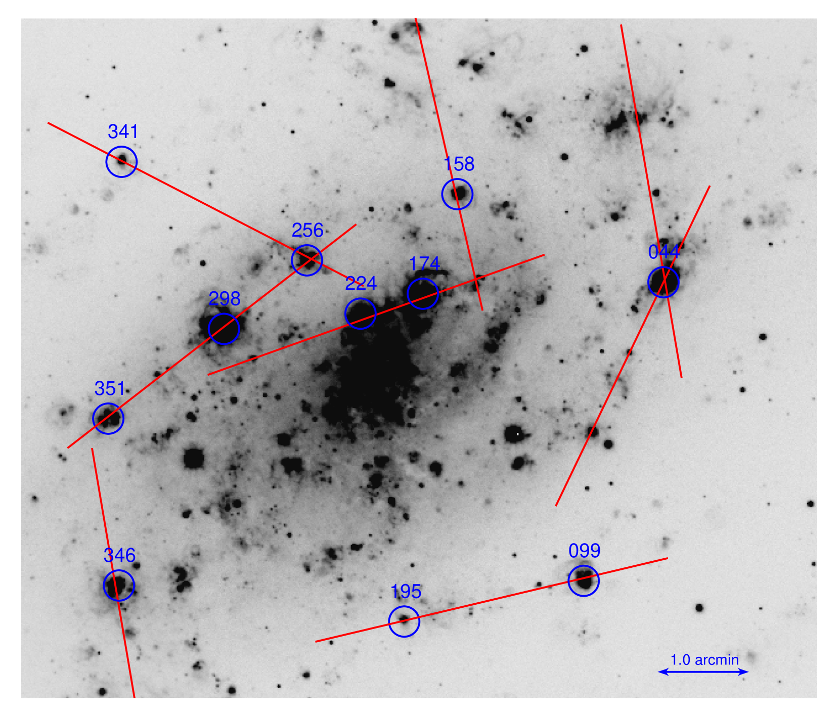
Figure 1.— Continuum-subtracted H$\alpha$ narrowband image of NGC 2403, taken with the 2.1 m telescope at Kitt Peak National Observatory. Blue circles enclose the H ii regions studied in this paper, and the identification number of each H ii region is quoted from Sivan et al. (1990). The positions of long-slit spectroscopic observations are shown as red solid lines, which overlaid the H ii regions. The scale in the bottom right corner indicates the 1$\arcmin$.0 length. North is at the up and east is to the left.

We selected 11 H ii regions, bright and large enough for spatially resolved studies, inside NGC 2403 from the catalog of Sivan et al. (1990, hereafter denoted as S90) as the sample. Their identification numbers in S90 are 044, 099, 158, 174, 195, 224, 256, 298, 341, 346, and 351, respectively. Spectroscopic observations were taken during seven nights in the years 2007 and 2008, with the 2.16 m telescope mounted at XingLong station of National Astronomical Observatories of China (Fan et al., 2016), as part of a spectroscopic survey of H ii regions in nearby galaxies (Kong et al., 2014, Lin et al. 2018, in preparation). The OMR (Opto-Mechanics Research Inc.) long-slit spectrograph, equipped with a TEKTRONIX TEK1024 AR-coated back-illuminated CCD and a grating of 300 lines per millimeter (i.e., 200 Å mm^-1) blazed at 5500 Å, were used to obtain spectra with a wavelength range of 3500$-$8000 Å and a spectral resolution of 500$-$550 (defined by $\lambda/\Delta\lambda$) at 5000 Å. The length of the spectrographic slit is 4$\arcmin$. The slit width was adjusted to 2$\arcsec$.5 in accordance with the local seeing disk.

Exposure time for each H ii region was $1800\times 2$ or $1200\times 3$ seconds. The slit was rotated to intersect as many H ii regions as possible at every exposure. Figure 1 shows spatial positions of the H ii regions in NGC 2403 and the orientation of the slit during each observation.

Instrument bias and dome flats were recorded at the beginning and the end of every night. A He-Ar lamp was observed after every exposure of the objects for wavelength calibrations. Spectrophotometric standards were selected from the catalog of International Reference Stars (IRS, Corbin & Warren, 1991) and observed several times at every night for flux calibrations.

Table 1 lists basic properties of the H ii regions and the information about the observations. We observed the No. 044 H ii region twice with two different position angles of the slit. The two observations are identified as 044a and 044b, respectively, as shown in Table 1 and Figure 2.

Table 1Basic Properties for the H ii Regions and Information About the Observations

ID.	R.A.	Decl.	$F$(H$\alpha$)	Observation	Exposure	Standard	Slit Angle	Airmass
	(J2000.0)	(J2000.0)		Date	Time	Stars
(1)	(2)	(3)	(4)	(5)	(6)	(7)	(8)	(9)
044a	07 36 20.0	+65 37 07	24.442	2008 Jan 01	1800 $\times$ 2	HD19445	9.2	1.1064
044b	07 36 20.0	+65 37 07	24.442	2008 Jan 06	1800 $\times$ 2	HD19445	$-$26.1	1.1055
099	07 36 28.8	+65 33 51	5.460	2008 Jan 04	1800 $\times$ 2	HE3	$-$77.5	1.1422
158	07 36 41.8	+65 38 06	2.689	2008 Jan 29	1200 $\times$ 3	HILTNER600	13.0	1.1524
174	07 36 45.6	+65 37 01	19.819	2008 Jan 07	1800 $\times$ 2	G191B2B	$-$71.0	1.1218
195	07 36 48.0	+65 33 26	0.317	2008 Jan 04	1800 $\times$ 2	HE3	$-$77.5	1.1422
244	07 36 52.2	+65 36 21	9.878	2008 Jan 07	1800 $\times$ 2	G191B2B	$-$71.0	1.1218
256	07 36 57.8	+65 36 24	4.940	2008 Jan 01	1200 $\times$ 3	HE3	63.0	1.1124
298	07 36 06.7	+65 36 39	30.010	2007 Jan 18	1800 $\times$ 2	G191B2B	$-$53.0	1.1059
341	07 37 17.5	+65 38 29	1.786	2008 Jan 01	1200 $\times$ 3	HE3	63.0	1.1124
346	07 37 18.1	+65 33 50	3.049	2008 Jan 01	1800 $\times$ 2	FEIGE34	9.2	1.1588
351	07 37 19.2	+65 35 40	1.601	2007 Jan 18	1800 $\times$ 2	G191B2B	$-$53.0	1.1059

Note. — Columns: (1) Identification numbers of the H ii regions; (2) Right ascension in the format of hour minute second; (3) Declination in the format of degree minute second; (4) H$\alpha$ flux in units of $10^{-13}~{}\mathrm{ergs~{}s^{-1}~{}cm^{-2}}$; (5) Observation dates in the format of year month date; (6) Exposure time in units of seconds; (7) Standard stars selected from the IRS catalog (Corbin & Warren, 1991); (8) Rotation angle of the spectrographic slit in units of degrees; (9) Airmass at each slit position.

3. DATA REDUCTION AND MEASUREMENTS

The raw data were reduced by using the IRAF software. After conventional steps of data reduction including bias subtraction, flat-field correction, and cosmic-ray removal (details of the processes will be presented in Lin et al. 2018, in preparation), we extract spectra radially for each H ii region by employing rectangular apertures on the slit. The size of the apertures is set to $3\arcsec.0\times 2\arcsec.5$, corresponding to a physical scale of $66\times 55~{}\mathrm{pc}^{2}$, approximately, with the distance of 3.5 Mpc adopted for NGC 2403 (Vinkó et al., 2006). During the radial spectra extraction, the first aperture was placed at the position of the H$\alpha$ emission peak in a nebula and defined as the central aperture; other apertures were placed along the slit at both sides of the central aperture with no gap between every two adjacent apertures; the number of the apertures applied to a nebula depends on the extension scale of H$\alpha$ emission along the spatial axis in the spatial-dispersion plane of the raw data; the outmost aperture at each side was placed by visually determining the outskirts of the H$\alpha$ profile through the interactive window of IRAF. For each H ii region, we also employed a large aperture integrating all of the 3 arcsec length apertures for extracting an integrated spectrum. Figure 2 illustrates the positions of the apertures placed on the H ii regions studied in our work. During the extraction of spectra from the apertures, we traced the trajectories along the dispersion axis, by applying a common function to all apertures in the same H ii region. Continuum points along the trace were obtained by summing enough dispersion lines and sampled to fit the tracing function manually under the IRAF interactive mode. Background levels were estimated from blank areas on the slit and subtracted from the object spectra.

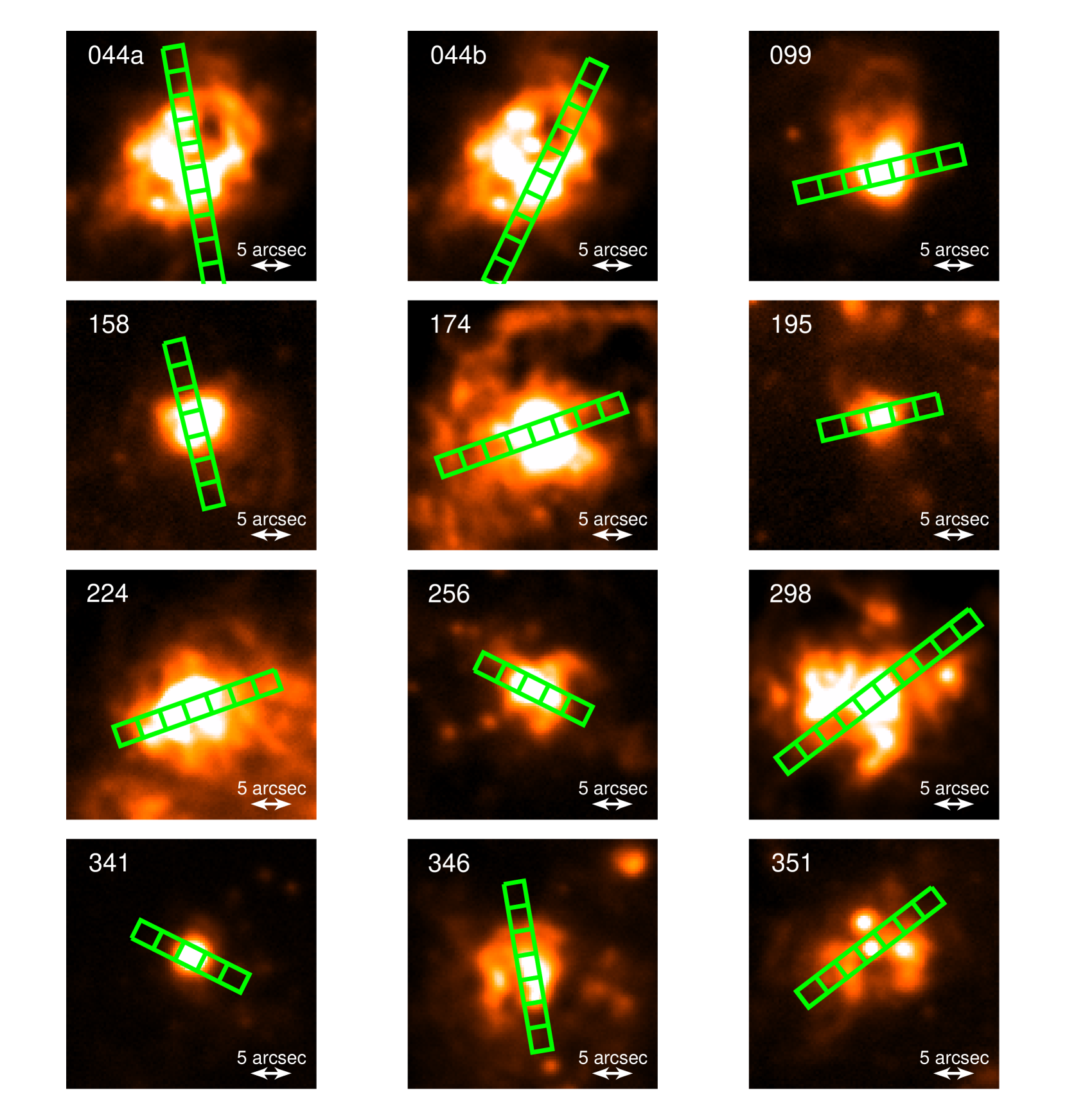
Figure 2.— Continuum-subtracted H$\alpha$ narrowband images of the H ii regions studied in this paper, intercepted from the image displayed in Figure 1. Green boxes represent rectangular apertures used for extracting spectra on the slit. In each panel, the identification number of the H ii region is displayed in the top left corner; the spatial scale in the bottom right corner indicates the 5$\arcsec$ length; north is at the up and east is to the left.

The dispersion of the extracted spectra was calibrated to wavelength by comparing with the spectra of the He-Ar lamp. Flux calibrations were performed by adopting the spectra of the standard stars and the atmospheric extinction curve at Xinglong station. All the spectra were corrected for Galactic foreground extinction, with the Cardelli et al. (1989) extinction curve and the total-to-selective extinction ratio $R_{\mathrm{V}}=3.1$ is utilized. The color excess of Galactic extinction $E(\mathrm{B}-\mathrm{V})_{\mathrm{GAL}}=0.04$ mag for NGC 2403 was obtained from the Schlegel et al. (1998) Galactic dust map. Calibrated spectra for the No. 044a H ii region are displayed in Figure 3 as a representative example of our spectral data.

Figure 3.— Observed spectra for all spectrophotometric units in the No. 044a H ii region as an example to convey the quality of the data obtained by our observations. The flux ($F_{\mathrm{\lambda}}$) in each spectrum is in units of $10^{-15}~{}\mathrm{ergs~{}s^{-1}~{}cm^{-2}~{}\AA^{-1}}$. $\Delta$L in each diagram identifies the spatial coordinate in units of arcsecond, where $\Delta$L = 0 represents the center of the H ii region defined in Section 3; the top left panel shows the spectra extracted from a large aperture integrating all the 3 arcsec length apertures.

We measured fluxes of the emission lines $\hbox{[O\,{\sc ii}]}\lambda 3727$, H$\gamma$, H$\beta$, $\hbox{[O\,{\sc iii}]}\lambda\lambda 4959,5007$, H$\alpha$, and $\hbox{[N\,{\sc ii}]}\lambda 6583$, by fitting Gaussian profiles through the MPFITEXPR algorithm (Markwardt, 2009). A major part of uncertainties in the fluxes were calculated by using the expression addressed in Castellanos et al. (2002); Bresolin et al. (2009): $\sigma_{\mathrm{line}}=\sigma_{\mathrm{con}}N_{\mathrm{pix}}^{1/2}[1+EW_{\mathrm{line}}/(N_{\mathrm{pix}}\Delta_{\mathrm{\lambda}})]^{1/2}$, where $\sigma_{\mathrm{line}}$ is the error in the flux of the emission line, $\sigma_{\mathrm{con}}$ is the standard deviation in the continuum near the emission line, $N_{\mathrm{pix}}$ is the number of pixels sampled in the measurements of the emission line, $EW_{\mathrm{line}}$ is the equivalent width of the emission line, and $\Delta_{\mathrm{\lambda}}$ is the minimum wavelength-interval (in units of Å per pixel) of the spectral data. Errors in the Gaussian fitting were also combined into final uncertainties in the emission-line fluxes.

All the fluxes were then corrected for internal dust attenuation of NGC 2403, by means of the Balmer decrement H$\alpha$/H$\beta$ (Osterbrock & Ferland, 2006), on assumption of the Fitzpatrick (1999) attenuation/extinction curve, the total-to-selective attenuation ratio $R_{\mathrm{V}}=3.1$, and the intrinsic H$\alpha$-to-H$\beta$ ratio equal to 2.86 (Hummer & Storey, 1987). Figure 4 shows radial profiles of the observed flux ratios H$\alpha$/H$\beta$, H$\alpha$/H$\gamma$, and H$\beta$/H$\gamma$ in all the H ii regions studied in this paper. A generally uniform trend of the three Balmer decrements can be seen. The data with observed $\mathrm{H}\alpha/\mathrm{H}\beta\leq 2.86$ were considered with no internal dust attenuation, and we did not perform the attenuation correction in this case. Application of a different attenuation curve will cause slight changes in final results, which will be inspected in the Appendix.

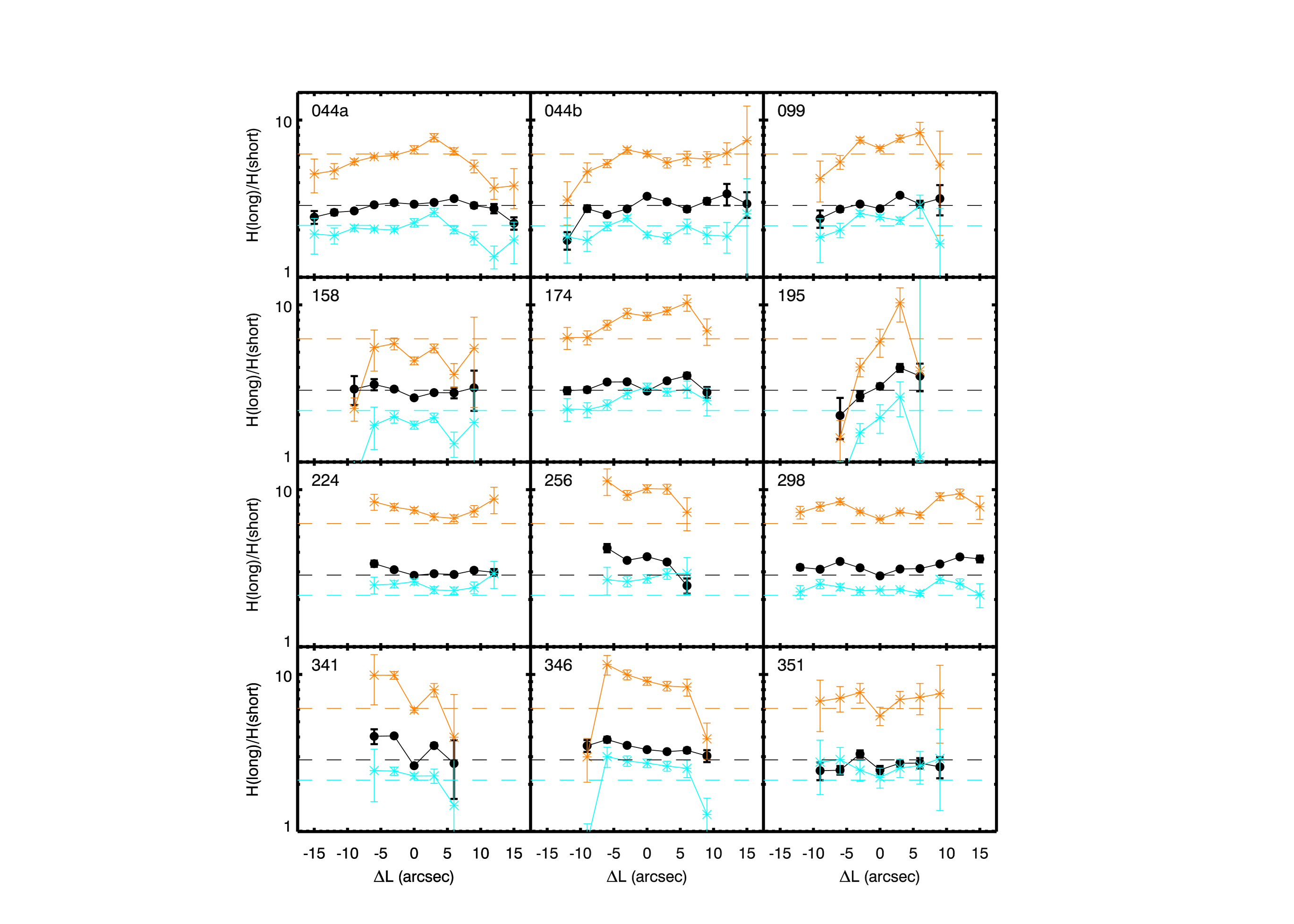
Figure 4.— Radial profiles of the observed flux ratios of H$\alpha$ to H$\beta$ (black filled circles), H$\alpha$ to H$\gamma$ (orange asterisks), and H$\beta$ to H$\gamma$ (cyan asterisks) in the individual H ii regions. Dashed lines mark the theoretically assumed lower limits for H$\alpha$/H$\beta$ (= 2.86, black), H$\alpha$/H$\gamma$ (= 6.09, orange), and H$\beta$/H$\gamma$ (= 2.13, cyan). In each panel, the abscissa is the spatial coordinate in units of arcseconds, where $\Delta$L = 0 represents the center of one H ii region defined in Section 3.

Table 2 presents the observed fluxes of the emission lines (relative to H$\beta$) for all the Spectrophotometric Units, and Table 3 presents the attenuation-corrected ones in the same form. We compared the attenuation-corrected flux ratios of $\hbox{[O\,{\sc ii}]}\lambda 3727$, $\hbox{[O\,{\sc iii}]}\lambda 4959$, $\hbox{[O\,{\sc iii}]}\lambda 5007$, and $\hbox{[N\,{\sc ii}]}\lambda 6583$, respectively, to H$\beta$ obtained through integrated measurements in our work, with those in Garnett et al. (1997, 1999); Berg et al. (2013), for the H ii regions commonly sampled in these studies. As depicted in Figure 5, the consistency between the normalized fluxes worked out by the different observations and measurements verifies the reliability of our work. Figure 6 shows radial profiles of attenuation-corrected luminosities in the form of logarithm for the emission lines, $\hbox{[O\,{\sc ii}]}\lambda 3727$, H$\beta$, $\hbox{[O\,{\sc iii}]}\lambda\lambda 4959,5007$, H$\alpha$, and $\hbox{[N\,{\sc ii}]}\lambda 6583$ in the H ii regions. The distributions of the luminosities are similar in general trend but distinct in detailed gradient for the different emission lines in each panel of the figure. The disparity between the gradients is likely to correlate with different sensitivities of these emission lines to the degree of ionization, which will be discussed in Section 5.

Table 2Observed Emission-line Fluxes for the Spectrophotometric Units

ID.	H$\beta$	$\hbox{[O\,{\sc ii}]}\lambda 3727$/H$\beta$	H$\gamma$/H$\beta$	$\hbox{[O\,{\sc iii}]}\lambda 4959$/H$\beta$	$\hbox{[O\,{\sc iii}]}\lambda 5007$/H$\beta$	H$\alpha$/H$\beta$	$\hbox{[N\,{\sc ii}]}\lambda 6583$/H$\beta$
044a_0	33.76 $\pm$ 0.66	3.00 $\pm$ 0.16	0.45 $\pm$ 0.03	0.49 $\pm$ 0.02	1.55 $\pm$ 0.04	2.92 $\pm$ 0.06	0.37 $\pm$ 0.01
044a_-3	70.74 $\pm$ 0.69	2.69 $\pm$ 0.08	0.50 $\pm$ 0.01	0.72 $\pm$ 0.01	2.18 $\pm$ 0.02	2.98 $\pm$ 0.03	0.32 $\pm$ 0.01
044a_-6	77.01 $\pm$ 0.68	2.69 $\pm$ 0.07	0.49 $\pm$ 0.01	0.71 $\pm$ 0.01	2.13 $\pm$ 0.02	2.89 $\pm$ 0.03	0.29 $\pm$ 0.01
044a_-9	29.23 $\pm$ 0.43	3.26 $\pm$ 0.13	0.49 $\pm$ 0.02	0.55 $\pm$ 0.01	1.62 $\pm$ 0.03	2.64 $\pm$ 0.04	0.36 $\pm$ 0.01
044a_-12	8.21 $\pm$ 0.30	3.52 $\pm$ 0.39	0.54 $\pm$ 0.06	0.37 $\pm$ 0.03	1.03 $\pm$ 0.05	2.58 $\pm$ 0.10	0.44 $\pm$ 0.03
044a_-15	3.09 $\pm$ 0.27	3.28 $\pm$ 0.86	0.53 $\pm$ 0.14	0.26 $\pm$ 0.08	0.79 $\pm$ 0.11	2.41 $\pm$ 0.23	0.39 $\pm$ 0.07
044a_3	27.22 $\pm$ 0.50	3.46 $\pm$ 0.17	0.39 $\pm$ 0.02	0.36 $\pm$ 0.02	1.05 $\pm$ 0.03	2.99 $\pm$ 0.06	0.43 $\pm$ 0.01
044a_6	19.93 $\pm$ 0.39	4.40 $\pm$ 0.21	0.50 $\pm$ 0.03	0.35 $\pm$ 0.02	1.01 $\pm$ 0.03	3.16 $\pm$ 0.07	0.49 $\pm$ 0.02
044a_9	8.67 $\pm$ 0.31	5.02 $\pm$ 0.47	0.56 $\pm$ 0.05	0.29 $\pm$ 0.03	0.86 $\pm$ 0.04	2.86 $\pm$ 0.11	0.51 $\pm$ 0.03
044a_12	4.38 $\pm$ 0.28	4.24 $\pm$ 0.76	0.74 $\pm$ 0.12	0.28 $\pm$ 0.06	0.73 $\pm$ 0.07	2.74 $\pm$ 0.19	0.50 $\pm$ 0.06
044a_15	3.48 $\pm$ 0.29	2.98 $\pm$ 0.68	0.58 $\pm$ 0.17	0.22 $\pm$ 0.07	0.61 $\pm$ 0.08	2.21 $\pm$ 0.20	0.44 $\pm$ 0.07
044a_wh	289.11 $\pm$ 1.72	2.93 $\pm$ 0.05	0.43 $\pm$ 0.01	0.61 $\pm$ 0.01	1.79 $\pm$ 0.01	2.88 $\pm$ 0.02	0.35 $\pm$ 0.00
$\cdots$

Note. — The fluxes in this table are in units of $10^{-15}~{}\mathrm{ergs~{}s^{-1}~{}cm^{-2}}$ and not corrected for internal dust attenuation. This table is available in its entirety in the online journal. A portion is shown here for guidance regarding its form and content.

It is worth pointing out that, in spectroscopic observations, apparent positions of observed objects are likely to be shifted by atmospheric refraction. The displacements of apparent from true positions will increase at larger airmasses or through shorter wavelength channels, or with a position-angle closer to 90^∘ for slit-spectrographs specifically. Notwithstanding, in our work, given that all the objects were observed near the zenith, at the airmasses $\sim 1.11-1.15$ as shown in Table 1, the impacts of atmospheric refraction are supposed to be trivial. In this case, during the process of data reduction, we did not correct the effects of the differential atmospheric refraction. Readers are referred to Filippenko (1982) for a comprehensive introduction about atmospheric refraction and its influences on slit spectrometry.

4. RESULTS

With the reduction and the measurements of the data described above, we derive oxygen abundances for each of the spectrophotometric units in the H ii regions from the four widely used strong-line indices, $R23$, $N2O2$, $N2$, and $O3N2$. These indices have been diversely calibrated to oxygen abundance, through empirical fits of not only observed relationships between $T_{\mathrm{e}}$ and the indices but also theoretical grids from photoionization models. The calibrations adopted in our work are listed as follows.

The $R23$ calibration addressed in Kobulnicky et al. (1999, hereafter denoted as $R23_{\mathrm{K99}}$),

$$12+\log(\mathrm{O/H})_{\mathrm{low}}=12.0-4.944+0.767x+0.602x^{2}$$ (1)

$$-y(0.29+0.332x-0.331x^{2}),$$

$$12+\log(\mathrm{O/H})_{\mathrm{high}}=12.0-2.939-0.2x-0.237x^{2}$$ (2)

$$-0.305x^{3}-0.0283x^{4}$$

$$-y(0.0047-0.0221x-0.102x^{2}-0.0817x^{3}-0.00717x^{4}),$$

where $x=\log[(\hbox{[O\,{\sc ii}]}\lambda 3727+\hbox{[O\,{\sc iii}]}\lambda\lambda 4959,5007)/\mathrm{H}\beta]$, $y=\log(\hbox{[O\,{\sc iii}]}\lambda\lambda 4959,5007/\hbox{[O\,{\sc ii}]}\lambda 3727)$;

The $R23$ calibration addressed in Pilyugin & Thuan (2005, hereafter denoted as $R23_{\mathrm{P05}}$),

$$12+\log(\mathrm{O/H})_{\mathrm{low}}=\frac{x+106.4+106.8y-3.40y^{2}}{17.72+6.60y+6.95y^{2}-0.302x},$$ (3)

$$12+\log(\mathrm{O/H})_{\mathrm{high}}=\frac{x+726.1+842.2y+337.5y^{2}}{85.96+82.76y+43.98y^{2}+1.793x},$$ (4)

where $x=(\hbox{[O\,{\sc ii}]}\lambda 3727+\hbox{[O\,{\sc iii}]}\lambda\lambda 4959,5007)/\mathrm{H}\beta$, $y=\hbox{[O\,{\sc iii}]}\lambda\lambda 4959,5007/(\hbox{[O\,{\sc ii}]}\lambda 3727+\hbox{[O\,{\sc iii}]}\lambda\lambda 4959,5007)$;

The $N2O2$ calibration addressed in Kewley & Dopita (2002, hereafter denoted as $N2O2_{\mathrm{K02}}$),

$$12+\log(\mathrm{O/H})=\log(1.54020+1.26602x+0.167977x^{2})+8.93,$$ (5)

where $x=\log(\hbox{[N\,{\sc ii}]}\lambda 6583/\hbox{[O\,{\sc ii}]}\lambda\lambda 3727)$;

The $N2O2$ calibration addressed in Bresolin (2007, hereafter denoted as $N2O2_{\mathrm{B07}}$),

$$12+\log(\mathrm{O/H})=8.66+0.36x-0.17x^{2},$$ (6)

where $x=\log(\hbox{[N\,{\sc ii}]}\lambda 6583/\hbox{[O\,{\sc ii}]}\lambda\lambda 3727)$;

The $N2$ calibration addressed in Pettini & Pagel (2004, hereafter denoted as $N2_{\mathrm{P04}}$),

$$12+\log(\mathrm{O/H})=9.37+2.03x+1.26x^{2}+0.32x^{3},$$ (7)

where $x=\log(\hbox{[N\,{\sc ii}]}\lambda 6583/\mathrm{H}\alpha)$;

The $O3N2$ calibration addressed in Pettini & Pagel (2004, hereafter denoted as $O3N2_{\mathrm{P04}}$),

$$12+\log(\mathrm{O/H})=8.73-0.32x,$$ (8)

where $x=\log[(\hbox{[O\,{\sc iii}]}\lambda 5007/\mathrm{H}\beta)/(\hbox{[N\,{\sc ii}]}\lambda 6583/\mathrm{H}\alpha)]$.

Since the $R23$ diagnostics suffer from a double-value problem (i.e., a fixed value for $R23$ corresponds to both a low value and a high value for $12+\log(\mathrm{O/H})$), we choose the upper branch of the $R23$ diagnostics throughout the work, except for the No. 158 H ii region behaving with apparent features of low metallicity to which we apply the lower branch, so as to avoid the degeneracy, in accordance with our existing knowledge cognizing NGC 2403 as a metal-rich galaxy. There are in total six sets of empirical oxygen abundances obtained for each nebula in our work. Among all the calibrations listed above, $R23_{\mathrm{P05}}$, $N2O2_{\mathrm{B07}}$, $N2_{\mathrm{P04}}$, and $O3N2_{\mathrm{P04}}$ are developed through observational approaches, while $R23_{\mathrm{K99}}$ and $N2O2_{\mathrm{K02}}$ are formulated theoretically on the basis of photoionization models. Some estimates from $R23$ or $N2O2$ are defined to be invalid. The invalidity of $R23$ occurs when the upper branch of the $R23$ diagnostics results in low abundances (or the lower branch leads to high values for the No. 158 H ii region); at the same time, estimates from $N2O2$ are picked out of valid results if $N2O2\leq 1.2$, since the calibrations of $N2O2$ were carried out with high-metallicity samples, or high-metallicity zones in model grids, and applicable to $N2O2>1.2$ for reliable estimates (Kewley & Dopita, 2002; Bresolin, 2007).

Figure 7 shows radial profiles of these ”strong-line” abundances in the H ii regions. The invalid estimates from $R23$ or $N2O2$ are marked in gray in the diagrams, including the rightmost $R23$ data points from the No. 099 H ii region, all the $R23$ and $N2O2$ data points from the No. 158 H ii region, the rightmost $R23_{\mathrm{P05}}$ data point and the $\Delta\mathrm{L}=\pm 3$ $N2O2$ data points from the No. 341 H ii region. Also in this figure, we do not plot the leftmost data points in the $N2O2$, $N2$, and $O3N2$ profiles for the No. 195 H ii region as well as the whole $N2O2$, $N2$, and $O3N2$ profiles for the No. 351 H ii region, because the $\hbox{[N\,{\sc ii}]}\lambda 6583$ emission lines were not well deblended from H$\alpha$ for these spectra in the flux measurements.

Systematic deviation between the diagnostics based on observations and models can be obviously seen from each of the diagrams in Figure 7. For the same spectral index, the calibrations on the basis of photoionization models leads to higher oxygen abundances (O/H) than the observation-based calibrations (i.e., $R23_{\mathrm{K99}}$ higher than $R23_{\mathrm{P05}}$, and $N2O2_{\mathrm{K02}}$ higher than $N2O2_{\mathrm{B07}}$) by 0.2$-$0.5 dex. The offsets appear to be constant at different nebular radii. On the other hand, the diagnostics with different spectral indices but identically calibrated via the observational relations with $T_{\mathrm{e}}$ (i.e., $R23_{\mathrm{P05}}$, $N2O2_{\mathrm{B07}}$, $N2_{\mathrm{P04}}$, and $O3N2_{\mathrm{P04}}$) result in approximately comparable abundance levels. The excesses of the model-based ”strong-line” abundances to the observation-based ones have also been found in many other studies with integrated measurements of H ii regions (e.g., Kennicutt et al., 2003; Pilyugin et al., 2010; Pilyugin & Grebel, 2016) or galaxies as a whole (e.g., Liang et al., 2006; Kewley & Ellison, 2008; Zahid et al., 2012).

A remarkable feature in Figure 7 is the similarity and disparity between radial distributions of these ”strong-line” abundances. We can see from each diagram that, $R23_{\mathrm{K99}}$ and $N2O2_{\mathrm{K02}}$ track each other exactly; $N2O2_{\mathrm{B07}}$ follows $R23_{\mathrm{K99}}$ and $N2O2_{\mathrm{K02}}$ in the shape of the profile despite the offset; the upturns and the downtrends of $R23_{\mathrm{P05}}$ roughly correlate with those of $R23_{\mathrm{K99}}$, $N2O2_{\mathrm{K02}}$, and $N2O2_{\mathrm{B07}}$, but the fluctuation is more intensive, yielding a radial variation $>0.2$ dex in most cases (even up to 0.4 dex for No. 044a H ii region); the estimates derived from $N2$ and $O3N2$ present an apparent gradient, increasing from the center to the edge of each nebula by $\sim 0.2-0.3$ dex on average.

Table 3Attenuation-corrected Emission-line Fluxes for the Spectrophotometric Units

ID.	H$\beta$	$\hbox{[O\,{\sc ii}]}\lambda 3727$/H$\beta$	H$\gamma$/H$\beta$	$\hbox{[O\,{\sc iii}]}\lambda 4959$/H$\beta$	$\hbox{[O\,{\sc iii}]}\lambda 5007$/H$\beta$	H$\alpha$/H$\beta$	$\hbox{[N\,{\sc ii}]}\lambda 6583$/H$\beta$
044a_0	35.69 $\pm$ 2.22	3.04 $\pm$ 0.34	0.45 $\pm$ 0.05	0.49 $\pm$ 0.04	1.54 $\pm$ 0.13	2.86 $\pm$ 0.21	0.36 $\pm$ 0.03
044a_-3	79.56 $\pm$ 2.55	2.78 $\pm$ 0.16	0.51 $\pm$ 0.03	0.71 $\pm$ 0.03	2.17 $\pm$ 0.09	2.86 $\pm$ 0.11	0.30 $\pm$ 0.01
044a_-6	79.36 $\pm$ 2.33	2.71 $\pm$ 0.14	0.50 $\pm$ 0.02	0.71 $\pm$ 0.03	2.13 $\pm$ 0.09	2.86 $\pm$ 0.10	0.29 $\pm$ 0.01
044a_-9	29.23 $\pm$ 0.43	3.26 $\pm$ 0.13	0.49 $\pm$ 0.02	0.55 $\pm$ 0.01	1.62 $\pm$ 0.03	2.64 $\pm$ 0.04	0.36 $\pm$ 0.01
044a_-12	8.21 $\pm$ 0.30	3.52 $\pm$ 0.39	0.54 $\pm$ 0.06	0.37 $\pm$ 0.03	1.03 $\pm$ 0.05	2.58 $\pm$ 0.10	0.44 $\pm$ 0.03
044a_-15	3.09 $\pm$ 0.27	3.28 $\pm$ 0.86	0.53 $\pm$ 0.14	0.26 $\pm$ 0.08	0.79 $\pm$ 0.11	2.41 $\pm$ 0.23	0.39 $\pm$ 0.07
044a_3	30.94 $\pm$ 1.87	3.60 $\pm$ 0.38	0.39 $\pm$ 0.04	0.36 $\pm$ 0.03	1.05 $\pm$ 0.09	2.86 $\pm$ 0.20	0.41 $\pm$ 0.03
044a_6	26.66 $\pm$ 1.71	4.78 $\pm$ 0.53	0.52 $\pm$ 0.06	0.34 $\pm$ 0.03	1.00 $\pm$ 0.09	2.86 $\pm$ 0.22	0.44 $\pm$ 0.04
044a_9	8.69 $\pm$ 1.00	5.02 $\pm$ 1.01	0.56 $\pm$ 0.11	0.29 $\pm$ 0.05	0.86 $\pm$ 0.14	2.86 $\pm$ 0.39	0.51 $\pm$ 0.07
044a_12	4.38 $\pm$ 0.28	4.24 $\pm$ 0.76	0.74 $\pm$ 0.12	0.28 $\pm$ 0.06	0.73 $\pm$ 0.07	2.74 $\pm$ 0.19	0.50 $\pm$ 0.06
044a_15	3.48 $\pm$ 0.29	2.98 $\pm$ 0.68	0.58 $\pm$ 0.17	0.22 $\pm$ 0.07	0.61 $\pm$ 0.08	2.21 $\pm$ 0.20	0.44 $\pm$ 0.07
044a_wh	295.18 $\pm$ 5.79	2.95 $\pm$ 0.10	0.43 $\pm$ 0.01	0.61 $\pm$ 0.02	1.79 $\pm$ 0.05	2.86 $\pm$ 0.07	0.35 $\pm$ 0.01
$\cdots$

Note. — The fluxes in this table are in units of $10^{-15}~{}\mathrm{ergs~{}s^{-1}~{}cm^{-2}}$ and have been corrected for internal dust attenuation. This table is available in its entirety in the online journal. A portion is shown here for guidance regarding its form and content.

In order to eliminate inevitable uncertainties propagated from the calibrations to the estimates during the derivation of the oxygen abundances and to analyze underlying causes of the diversity between the radial distributions in depth, we additionally plot radial profiles of the strong-line indices, $R23$, $N2O2$, $N2$, and $O3N2$, as well as $R2$ ( $\equiv$ $\log(\hbox{[O\,{\sc ii}]}\lambda 3727/\mathrm{H}\beta)$), $R3$ ( $\equiv$ $\log(\hbox{[O\,{\sc iii}]}\lambda\lambda 4959,5007/\mathrm{H}\beta)$), and $O3O2$ ( $\equiv$ $\log(\hbox{[O\,{\sc iii}]}\lambda\lambda 4959,5007/\hbox{[O\,{\sc ii}]}\lambda 3727)$, the other indices in the $R23$ diagnostics) for the H ii regions in Figure 8. Among the seven indices, $R2$, $R3$, and $N2$ represent relative fluxes for the collisionally excited lines $\hbox{[O\,{\sc ii}]}\lambda 3727$, $\hbox{[O\,{\sc iii}]}\lambda\lambda 4959,5007$, and $\hbox{[N\,{\sc ii}]}\lambda 6583$, respectively, which consolidate the indices $R23$, $N2O2$, $O3N2$, and $O3O2$ by means of certain combinations.

As can be seen from this figure, $R3$, $O3N2$, and $O3O2$ uniformly decrease with the nebular radius, while $R2$ and $N2$ increase from the center to the edge. In contrast to such obvious gradients, $R23$ and $N2O2$, in most cases of our study, appear with shallow distributions. It is easy to understand that, when combining $R2$ and $R3$ into $R23$, the opposite radial variations in the two indices will compensate the offsets between each other along the nebular radius and consequently flatten the $R23$ profile; similarly, a combination of $N2$ and $R2$ in a ratio form will also have a counteracting effect on the radial variation and generate $N2O2$ with a gentle or even no slope in the profile. Nevertheless, if the collisionally excited line in $R2$ or $R3$ or $N2$ is strong enough to effectively dominate the consolidated index $R23$ or $N2O2$, the radial profile of $R23$ or $N2O2$ is still likely to exhibit a gradient. In our work, this situation occurs in the Nos. 158 and 174 H ii regions, where $\hbox{[O\,{\sc ii}]}\lambda 3727$ is relatively overwhelming compared with other emission lines; $R23$ and $N2O2$ hence perform visible gradients as a result of the covariation with $R2$. On the other hand, the ratio of $R3$ to $N2$ (or $R2$) will inevitably produce an amplified radial variation, contributing the steepest gradients of $O3N2$ and $O3O2$ in all cases in Figure 8. The radial distributions of $R23$, $N2O2$, $N2$, $O3N2$, and $O3O2$ in our work coincide with earlier studies of the two H ii regions NGC 595 and NGC 588 inside M33, observed with integral field spectrographs, where $O3N2$, $N2$, and $O3O2$ obviously correlate with nebular radii, whereas $R23$ and $N2O2$ are constantly distributed from centers to edges (Relaño et al., 2010; Monreal-Ibero et al., 2011).

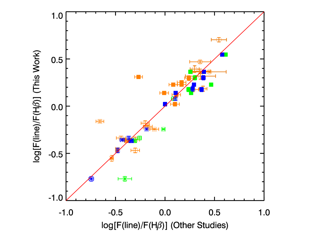
Figure 5.— Comparison of attenuation-corrected emission-line fluxes (relative to H$\beta$ flux) for the H ii regions obtained through integrated measurements in our work with those in previous studies, including Garnett et al. (1997, in orange), Garnett et al. (1999, in green), and Berg et al. (2013, in blue). The emission lines compared in this figure are $\hbox{[O\,{\sc ii}]}\lambda 3727$ (open circles), $\hbox{[O\,{\sc iii}]}\lambda 4959$ (open squares), $\hbox{[O\,{\sc iii}]}\lambda 5007$ (filled squares), and $\hbox{[N\,{\sc ii}]}\lambda 6583$ (asterisks). The line of unity is also shown as the red solid line.

Figure 8 provides a straightforward interpretation of the radial variations in the oxygen abundances in Figure 7, with a decrease or increase in relative fluxes for the collisionally excited lines at larger radii. Apart from the invalid data points from the Nos. 158 and 341 H ii regions as marked in gray in Figure 7, a complicated case appears in the index $R23$ from which the two estimates $R23_{\mathrm{K99}}$ and $R23_{\mathrm{P05}}$ clearly differ from each other in the radial fluctuation even if the offsets are neglected. In consideration of the consistency between $R23_{\mathrm{K99}}$, $N2O2_{\mathrm{K02}}$, and $N2O2_{\mathrm{B07}}$, the discrepancy of $R23_{\mathrm{P05}}$ from the three indices in the radial variations implies a possible problem lying in the $R23_{\mathrm{P05}}$ diagnostic. By comparing Figures 7 and 8 on a panel-by-panel basis, we find that the peaks or the valleys of $R23_{\mathrm{P05}}$ and $O3O2$ coincidentally occur one by one. Due to this behavior, we suspect that the $R23_{\mathrm{P05}}$ prescription is likely to overweigh $O3O2$ in terms of the parameterization and the formulation in Equations (3) and (4), compared to those in Equations (1) and (2) for $R23_{\mathrm{K99}}$ where the parameters $x$ and $y$ are actually different. We will attempt to make considerate inspections to validate or challenge this suspicion in our future work.

Besides the radial distributions presented above, the ”strong-line” abundances for the H ii regions with integrated measurements are also listed in Table 4. The deviation in the ”integrated” abundances for the same H ii region appears to be constant with uncertainties taken into account and not evidently related with other parameters. Integrated measurements of a large sample of H ii regions will be conducted and systematic differences between the strong-line diagnostics will be investigated in a separate study (Lin et al. 2018, in preparation). In this current work, we compare the results of the measurements by adopting large and small apertures. Table 5 lists the ”strong-line” abundances for the centers of the H ii regions (i.e., by employing the 3 arcsec length aperture). A comparison between Tables 4 and 5 manifests a trivial change within the range of error between the large- and small-aperture measurements, which suggests that the measurements with a small aperture are able to comply with the integrated measurements as long as the brightest part of the H ii region is enclosed.

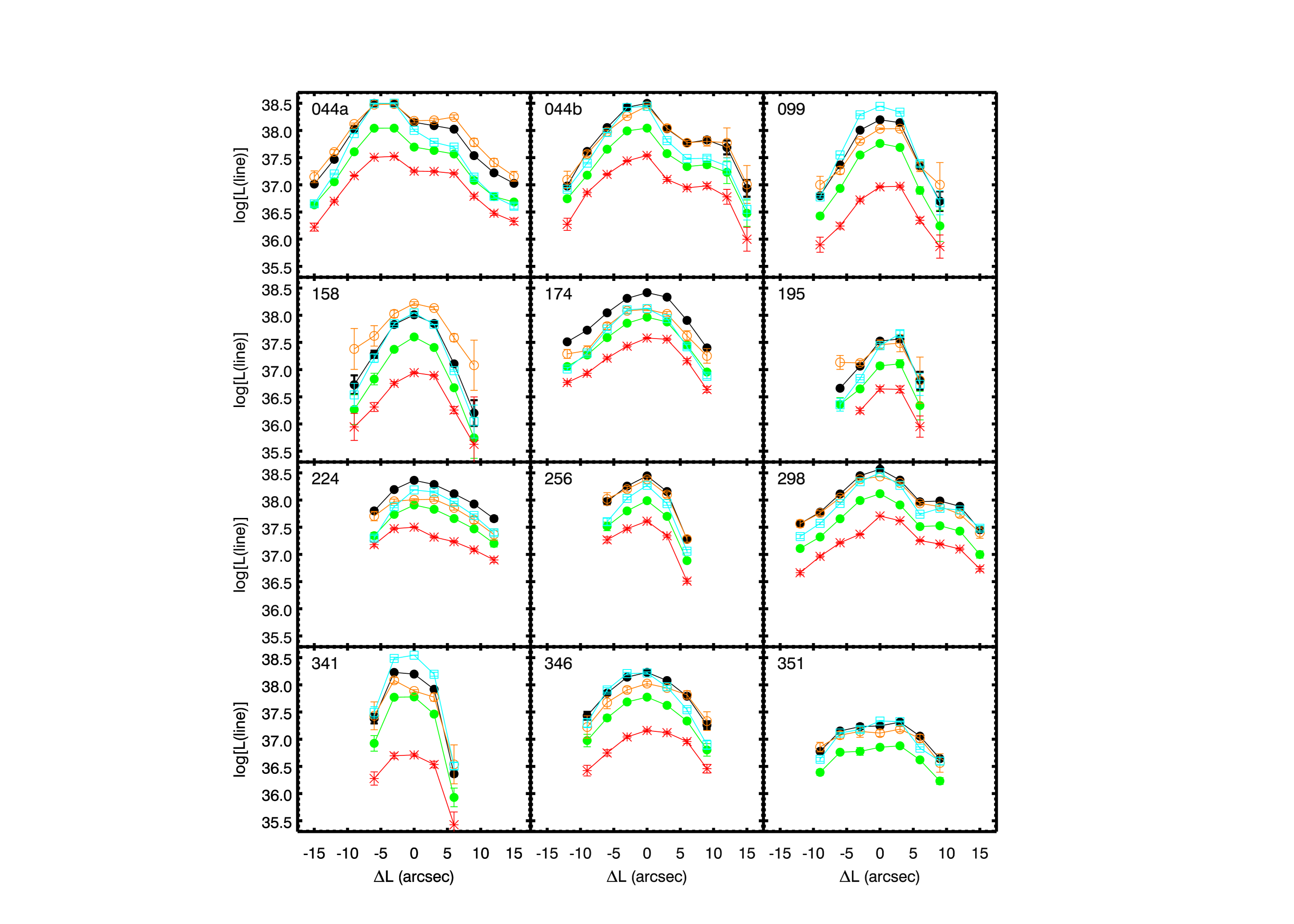
Figure 6.— Radial profiles of attenuation-corrected luminosities in the form of logarithm for the emission lines, $\hbox{[O\,{\sc ii}]}\lambda 3727$ (orange open circles), H$\beta$ (green filled circles), $\hbox{[O\,{\sc iii}]}\lambda\lambda 4959,5007$ (cyan open squares), H$\alpha$ (black filled circles), and $\hbox{[N\,{\sc ii}]}\lambda 6583$ (red asterisks), in the individual H ii regions. All the luminosities are in units of $\mathrm{ergs~{}s^{-1}}$) in the form of logarithm. In each panel, the abscissa is the spatial coordinate in units of arcsecond, where $\Delta$L = 0 represents the center of one H ii region defined in Section 3.

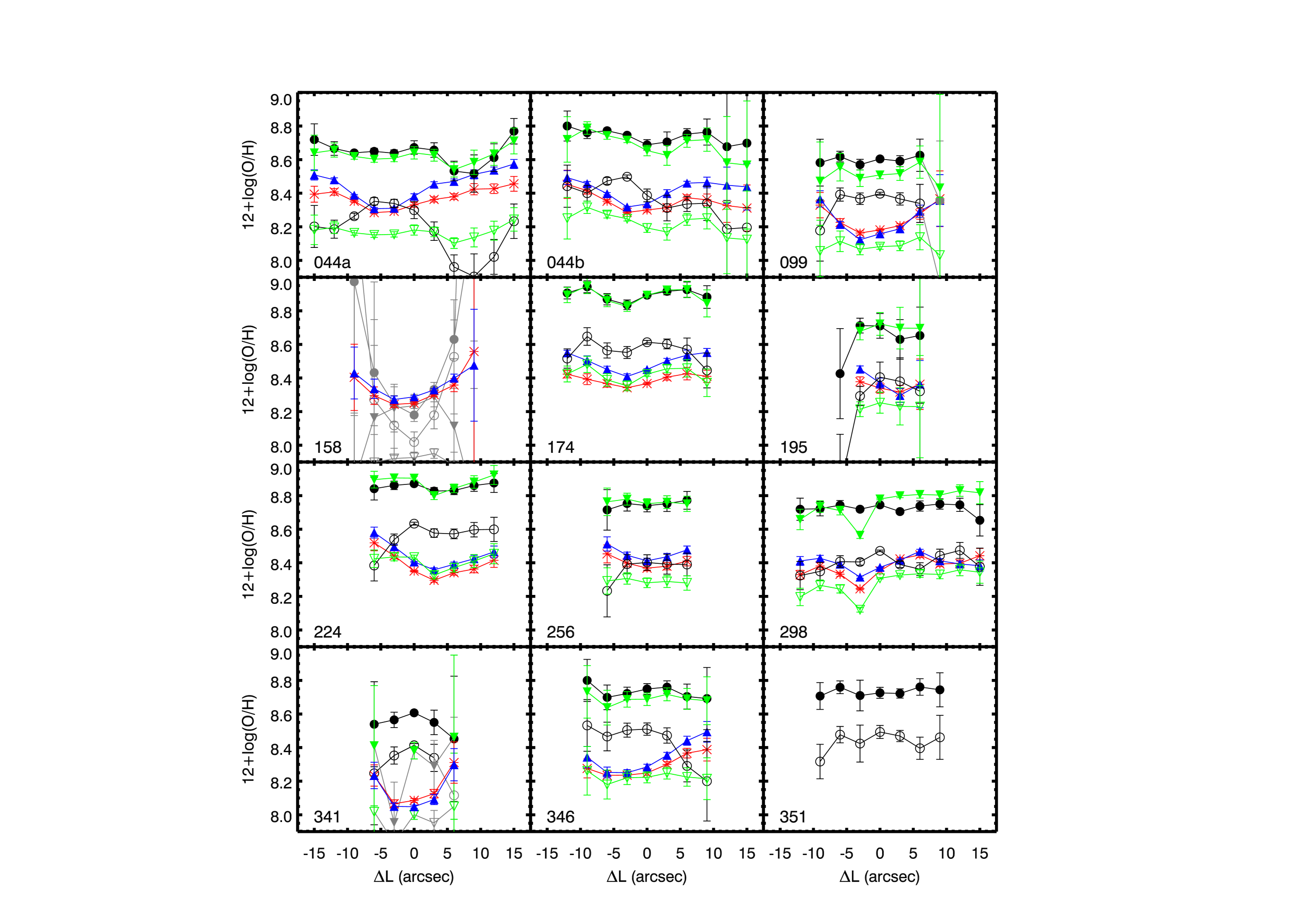
Figure 7.— Radial profiles of the oxygen abundances derived from $R23_{\mathrm{K99}}$ (black filled circles), $R23_{\mathrm{P05}}$ (black open circles), $N2_{\mathrm{P04}}$ (red asterisks), $O3N2_{\mathrm{P04}}$ (blue filled triangles), $N2O2_{\mathrm{K02}}$ (green filled upside-down triangles), and $N2O2_{\mathrm{B07}}$ (green open upside-down triangles) in the individual H ii regions. The gray color marks the data out of the calibration ranges, considered to be invalid results as explained in Section 4. In each panel, the abscissa is the spatial coordinate in units of arcseconds, where $\Delta$L = 0 represents the center of one H ii region defined in Section 3.

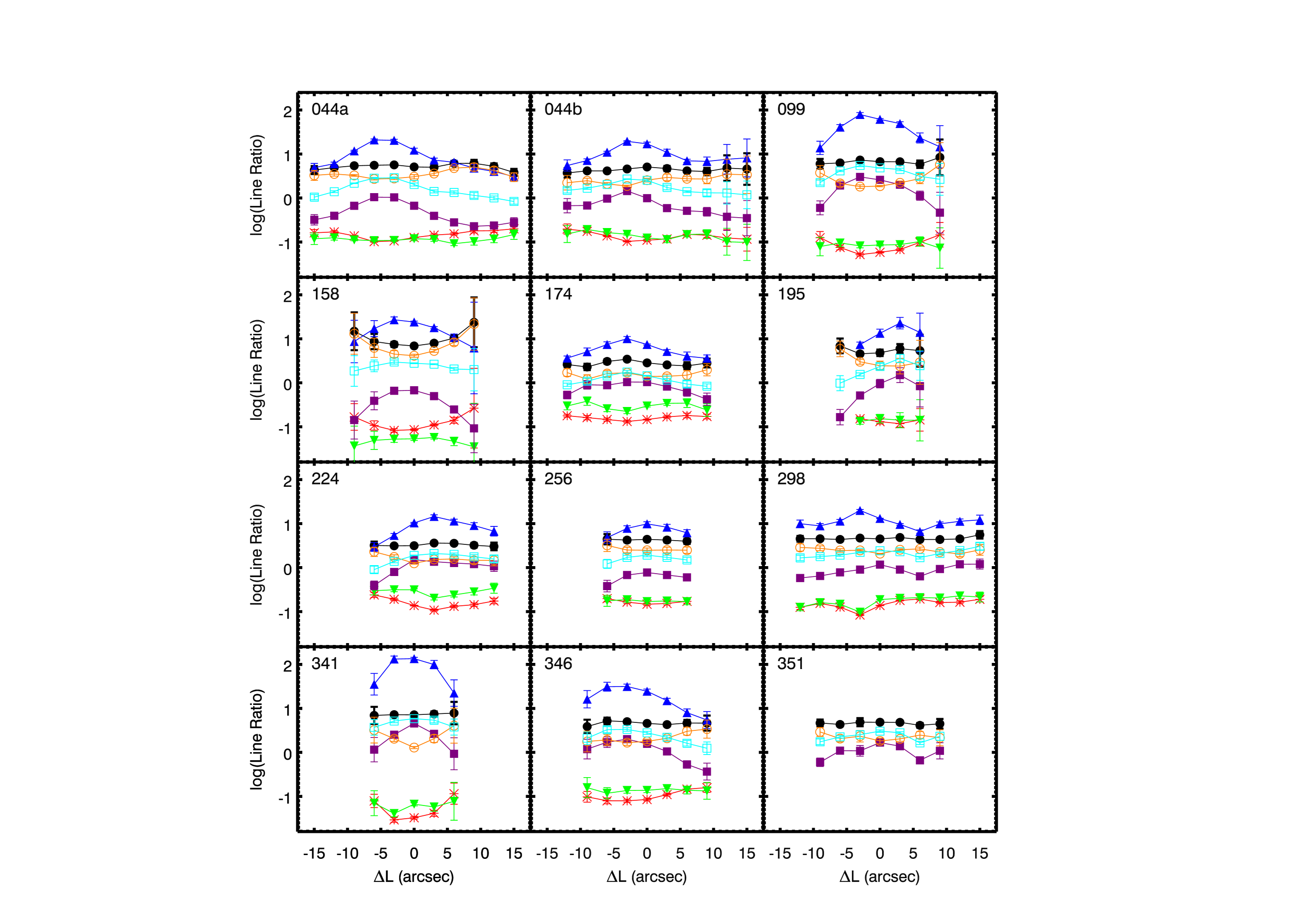
Figure 8.— Radial profiles of the spectral indices, $R23$ (black filled circles), $N2$ (red asterisks), $O3N2$ (blue filled triangles), $N2O2$ (green filled upside-down triangles), $R2$ (orange open circles), $R3$ (cyan open squares), and $O3O2$ (purple filled squares) in the individual H ii regions. In each panel, the abscissa is the spatial coordinate in units of arcseconds, where $\Delta$L = 0 represents the center of one H ii region defined in Section 3.

5. DISCUSSION

Table 4Empirical Oxygen Abundances ($12+\log(\mathrm{O/H})$) for the H ii Regions with Integrated Measurements

ID.	$R23_{\mathrm{K99}}$	$N2O2_{\mathrm{K02}}$	$R23_{\mathrm{P05}}$	$N2O2_{\mathrm{B07}}$	$O3N2_{\mathrm{P04}}$	$N2_{\mathrm{P04}}$
044a	8.655 $\pm$ 0.013	8.635 $\pm$ 0.012	8.317 $\pm$ 0.016	8.177 $\pm$ 0.010	8.356 $\pm$ 0.005	8.321 $\pm$ 0.005
044b	8.726 $\pm$ 0.017	8.702 $\pm$ 0.017	8.426 $\pm$ 0.020	8.236 $\pm$ 0.015	8.359 $\pm$ 0.007	8.315 $\pm$ 0.007
099	8.597 $\pm$ 0.018	8.513 $\pm$ 0.025	8.384 $\pm$ 0.020	8.084 $\pm$ 0.018	8.164 $\pm$ 0.008	8.187 $\pm$ 0.006
158	8.419 $\pm$ 0.025	8.205 $\pm$ 0.049	7.971 $\pm$ 0.032	7.915 $\pm$ 0.021	8.303 $\pm$ 0.005	8.269 $\pm$ 0.006
174	8.882 $\pm$ 0.013	8.879 $\pm$ 0.014	8.583 $\pm$ 0.017	8.408 $\pm$ 0.014	8.458 $\pm$ 0.008	8.372 $\pm$ 0.009
195	8.663 $\pm$ 0.071	8.677 $\pm$ 0.064	8.330 $\pm$ 0.089	8.214 $\pm$ 0.055	8.370 $\pm$ 0.026	8.345 $\pm$ 0.027
224	8.849 $\pm$ 0.011	8.885 $\pm$ 0.011	8.589 $\pm$ 0.014	8.414 $\pm$ 0.012	8.421 $\pm$ 0.007	8.373 $\pm$ 0.007
256	8.753 $\pm$ 0.027	8.770 $\pm$ 0.022	8.402 $\pm$ 0.034	8.298 $\pm$ 0.021	8.433 $\pm$ 0.012	8.384 $\pm$ 0.013
298	8.732 $\pm$ 0.008	8.781 $\pm$ 0.006	8.431 $\pm$ 0.009	8.309 $\pm$ 0.006	8.396 $\pm$ 0.003	8.378 $\pm$ 0.004
341	8.585 $\pm$ 0.027	8.320 $\pm$ 0.063	8.387 $\pm$ 0.030	7.967 $\pm$ 0.032	8.063 $\pm$ 0.013	8.095 $\pm$ 0.012
346	8.728 $\pm$ 0.023	8.678 $\pm$ 0.025	8.464 $\pm$ 0.027	8.214 $\pm$ 0.022	8.310 $\pm$ 0.010	8.273 $\pm$ 0.009
351	8.726 $\pm$ 0.018	…	8.456 $\pm$ 0.023	…	…	…

Note. — The table-head presents the six diagnostics adopted for estimating the oxygen abundances listed below.

Table 5Empirical Oxygen Abundances ($12+\log(\mathrm{O/H})$) for the Centers of the H ii Regions

ID.	$R23_{\mathrm{K99}}$	$N2O2_{\mathrm{K02}}$	$R23_{\mathrm{P05}}$	$N2O2_{\mathrm{B07}}$	$O3N2_{\mathrm{P04}}$	$N2_{\mathrm{P04}}$
044a	8.672 $\pm$ 0.040	8.640 $\pm$ 0.036	8.299 $\pm$ 0.051	8.181 $\pm$ 0.030	8.382 $\pm$ 0.015	8.331 $\pm$ 0.015
044b	8.688 $\pm$ 0.031	8.654 $\pm$ 0.031	8.387 $\pm$ 0.038	8.193 $\pm$ 0.026	8.336 $\pm$ 0.013	8.300 $\pm$ 0.012
099	8.604 $\pm$ 0.008	8.509 $\pm$ 0.023	8.397 $\pm$ 0.009	8.082 $\pm$ 0.016	8.158 $\pm$ 0.006	8.182 $\pm$ 0.006
158	8.509 $\pm$ 0.030	8.235 $\pm$ 0.067	8.120 $\pm$ 0.039	7.927 $\pm$ 0.030	8.288 $\pm$ 0.007	8.250 $\pm$ 0.008
174	8.893 $\pm$ 0.008	8.893 $\pm$ 0.012	8.613 $\pm$ 0.011	8.423 $\pm$ 0.012	8.451 $\pm$ 0.004	8.367 $\pm$ 0.006
195	8.710 $\pm$ 0.073	8.722 $\pm$ 0.068	8.405 $\pm$ 0.090	8.253 $\pm$ 0.062	8.370 $\pm$ 0.030	8.340 $\pm$ 0.031
224	8.871 $\pm$ 0.007	8.904 $\pm$ 0.011	8.633 $\pm$ 0.009	8.434 $\pm$ 0.011	8.405 $\pm$ 0.004	8.351 $\pm$ 0.005
256	8.740 $\pm$ 0.037	8.752 $\pm$ 0.030	8.402 $\pm$ 0.046	8.281 $\pm$ 0.029	8.412 $\pm$ 0.016	8.368 $\pm$ 0.016
298	8.745 $\pm$ 0.004	8.780 $\pm$ 0.005	8.471 $\pm$ 0.004	8.308 $\pm$ 0.004	8.373 $\pm$ 0.002	8.352 $\pm$ 0.003
341	8.607 $\pm$ 0.009	8.382 $\pm$ 0.049	8.414 $\pm$ 0.010	8.001 $\pm$ 0.028	8.048 $\pm$ 0.010	8.086 $\pm$ 0.012
346	8.749 $\pm$ 0.032	8.688 $\pm$ 0.037	8.510 $\pm$ 0.037	8.223 $\pm$ 0.033	8.285 $\pm$ 0.016	8.249 $\pm$ 0.013
351	8.726 $\pm$ 0.033	…	8.493 $\pm$ 0.039	…	…	…

Note. — The table-head presents the six diagnostics adopted for estimating the oxygen abundances listed below.

In this work, we confirm the systematic offsets between the empirical oxygen abundances separately estimated with the observation- and model-based prescriptions. Physical origins of the offsets are still unclear. Aside from inappropriate treatments of ionization structures in theoretical models, biased sampling of emission-line sources in the observation-based calibrations is suspected to be a possible cause (Kennicutt et al., 2003; Bresolin, 2007; Kewley & Ellison, 2008). The observational relationships between the strong lines and the $T_{\mathrm{e}}$-sensitive auroral lines are often obtained with integrated measurements of H ii regions or star-forming galaxies. However, due to temperature fluctuations within an ionized nebula, detected auroral lines in most cases actually indicate higher temperature and thus lower metallicity than measured strong lines for the same data point in calibration diagrams. Therefore, with the peak $T_{\mathrm{e}}$ referencing the averaged strong lines in a nebula, the empirical diagnostics are supposed to underestimate true oxygen abundances at certain degrees. The solution of this problem is to recalibrate the empirical abundance indicators by measuring both auroral and strong lines for identical positions inside one H ii region.

The radial variations in the empirical oxygen abundances, or more directly, the strong-line indices, are significant fruits of our investigation. It is not realistic for actual oxygen abundances to vary so sharply on a nebular scale ($\lesssim 330$ pc). Therefore, our results imply the existence of additional parameters affecting the widely used abundance indicators. The sensitivities of $\hbox{[O\,{\sc ii}]}\lambda 3727$, $\hbox{[O\,{\sc iii}]}\lambda\lambda 4959,5007$, and $\hbox{[N\,{\sc ii}]}\lambda 6583$ to ionization levels suggest the ionization parameter as a candidate to underlie the spectral indices, in addition to the oxygen abundance. Among these collisionally excited lines, $\hbox{[O\,{\sc iii}]}\lambda\lambda 4959,5007$ are more efficiently excited in regions with a high degree of ionization, while $\hbox{[O\,{\sc ii}]}\lambda 3727$ and $\hbox{[N\,{\sc ii}]}\lambda 6583$ are more related with a low-ionization state (Emerson, 1996; Osterbrock & Ferland, 2006). In this situation, a decrease in the ionization parameter is supposed to raise $R2$ and $N2$, to diminish $R3$, $O3N2$, and $O3O2$, and to ineffectively change $R23$ and $N2O2$, if intrinsic metallicities are constant. At the same time, ionization states are postulated to inherently decline at larger radii of an ionized nebula. In support of this postulation, 3-D nebular models configured with such an ionization structure have successfully reproduced 2-D multi-wavelength features of individual H ii regions (Pérez-Montero et al., 2011, 2014). As a consequence, the radial gradients of $N2$ and $O3N2$ in Figure 8 are consistent with the natural distribution of the ionization parameter within one H ii region and considered to be an imprint of the ionization parameter rather than the the oxygen abundance, whereas the flat profiles of $R23$ and $N2O2$ manifest the robustness of the two indices against ionization variations, which has been disclosed by several other observations of H ii regions in the Milky Way and the Magellanic Clouds (Kennicutt et al., 2000; Oey & Shields, 2000) as well as local galaxies (Bresolin, 2007; James et al., 2016), also in agreement with expectations of photoionization models (Kewley & Dopita, 2002; Dopita et al., 2013). Likewise, the different sensitivities of the emission lines to the radially decreasing ionization parameter offer an interpretation of the disparity between the gradients displayed in each panel of Figure 6, i.e., steeper for $\hbox{[O\,{\sc iii}]}\lambda\lambda 4959,5007$ and shallower for $\hbox{[O\,{\sc ii}]}\lambda 3727$ and $\hbox{[N\,{\sc ii}]}\lambda 6583$.

The reliability of $R23$ and $N2O2$, at least when the ionization parameter varies, which is the predominant situation in our study, is also reflected in our work by consistent fluctuations in the radial profiles of model-based $R23_{\mathrm{K99}}$ and $N2O2_{\mathrm{K02}}$ shown in each panel of Figure 7, albeit the same emission line $\hbox{[O\,{\sc ii}]}\lambda 3727$ is located in the numerator of one index ($R23$) but the denominator of the other ($N2O2$). In contrast to the proximate overlap between $R23_{\mathrm{K99}}$ and $N2O2_{\mathrm{K02}}$, $R23_{\mathrm{P05}}$ deviates from $N2O2_{\mathrm{B07}}$ by even up to 0.4 dex, as depicted in Figure 7. As a commonly accepted probe of ionization levels, $O3O2$ is combined with $R23$ into the diagnostics for correcting the influences of the ionization parameter on $R23$. However, in our work, the flat distributions of $R23$ in Figure 8 and the intensive fluctuations of $R23_{\mathrm{P05}}$ in Figure 8 suggest that, $R23$, neutralized by $R2$ and $R3$ though incompletely in many cases, appears not so sensitive to the degree of ionization as $N2$ and $O3N2$, and the ionization correction in the $R23_{\mathrm{P05}}$ diagnostic needs to be reexamined in a high variety of ionization states.

The failure of applying $N2$ and $O3N2$ to various ionization states has been predicted by photoionization models (e.g., Kewley & Dopita, 2002), yet there has not been direct observational evidence demonstrating the correlation of $N2$ or $O3N2$ with the ionization parameter. Nevertheless, observations of H ii regions in the Magellanic Clouds have revealed more spatially extended contours for low-ionization emission lines than high-ionization ones (Pellegrini et al., 2012), which actually implies potential deviation in abundance estimates from ionization-sensitive emission lines such as $\hbox{[O\,{\sc iii}]}\lambda\lambda 4959,5007$ and $\hbox{[N\,{\sc ii}]}\lambda 6583$. Despite this drawback of $N2$ and $O3N2$, in the case that ionization states are not quite variable, $N2$ and $O3N2$ are still applicable, in particular to heavily dust-obscured regions since both of the indices are independent of dust attenuation.

In a short summary, through spatially resolved spectrophotometry of 11 H ii regions in NGC 2403 and thereby naturally sampling various ionization states, our study corroborates the theoretical expectation and offers the observational evidence of the similarities and differences between the empirical diagnostics of the oxygen abundance. Further confirmation of the interpretations of the discrepancies, such as the temperature fluctuations and the ionization diversities, will rest on comparison of the empirical estimates with the $T_{\mathrm{e}}$-based oxygen abundance, which requires successful detection of the auroral lines. However, in this present work, for NGC 2403 with the metallicity $>0.5Z_{\odot}$ (Berg et al., 2013), the auroral lines are undetectable with the 2.16 m telescope, which hampers us to recalibrate the strong-line indices or obtain the internal distributions of $T_{\mathrm{e}}$ for the H ii regions. In future work, we plan to target metal-poor H ii regions in nearby galaxies or in the Milky Way, where the auroral lines are observable, aimed at an in-depth exploration on the factors affecting the empirical abundance diagnostics.

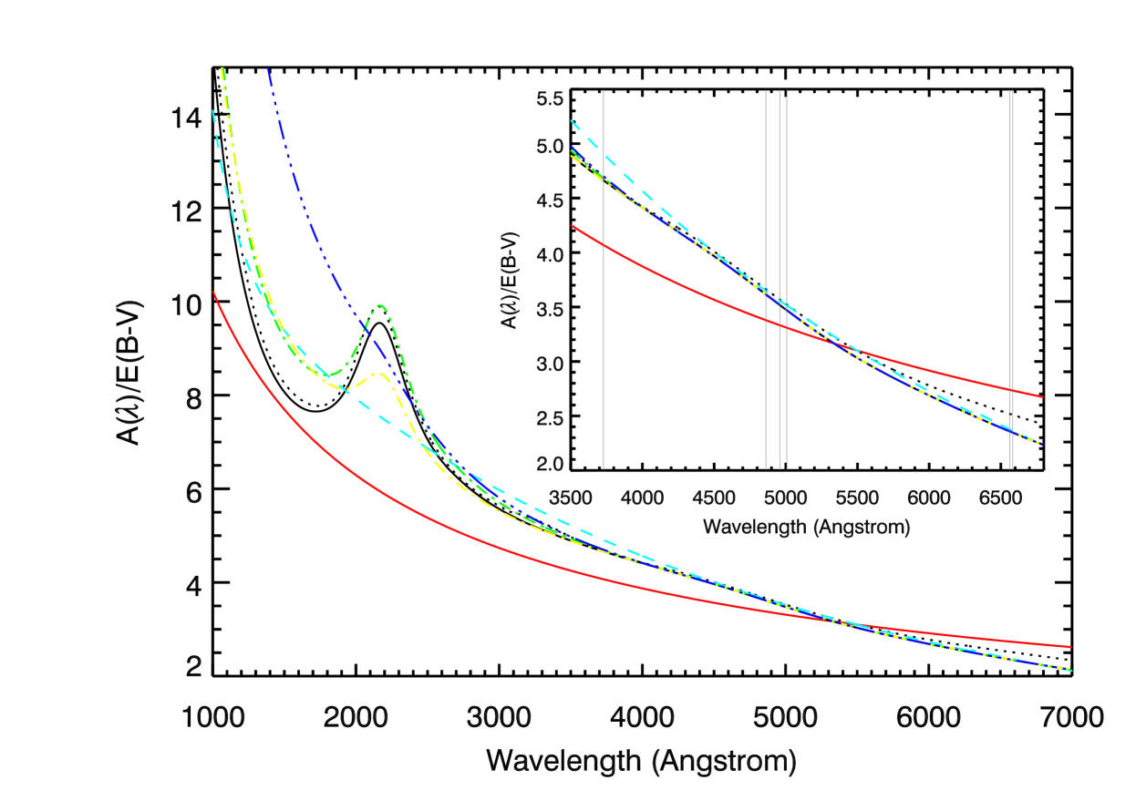
Figure 9.— Seven attenuation/extinction curves in a wavelength range from UV to optical bands with $R_{\mathrm{V}}=3.1$, including the Fitzpatrick (1999) curve (black solid line), the Calzetti et al. (2000) curve (cyan dashed line), the Cardelli et al. (1989) curve (black dotted line), the Gordon et al. (2003) curve for the Large Magellanic Cloud (green dotted-dashed line), the Gordon et al. (2003) curve for the supershell area in the Large Magellanic Cloud (yellow dotted-dashed line), the Gordon et al. (2003) curve for the Small Magellanic Cloud (blue triple-dotted-dashed line), and the Charlot & Fall (2000) curve of $\lambda^{-0.7}$ (red solid line). The internal panel is plotted to highlight the difference between these curves in the optical range relevant to our work, where the gray solid lines mark the wavelength-positions for the emission lines, $\hbox{[O\,{\sc ii}]}\lambda 3727$, H$\beta$, $\hbox{[O\,{\sc iii}]}\lambda\lambda 4959,5007$, H$\alpha$, and $\hbox{[N\,{\sc ii}]}\lambda 6583$, from left to right on the horizontal axis.

Appendix A AN INSPECTION OF DIFFERENT ATTENUATION CURVES

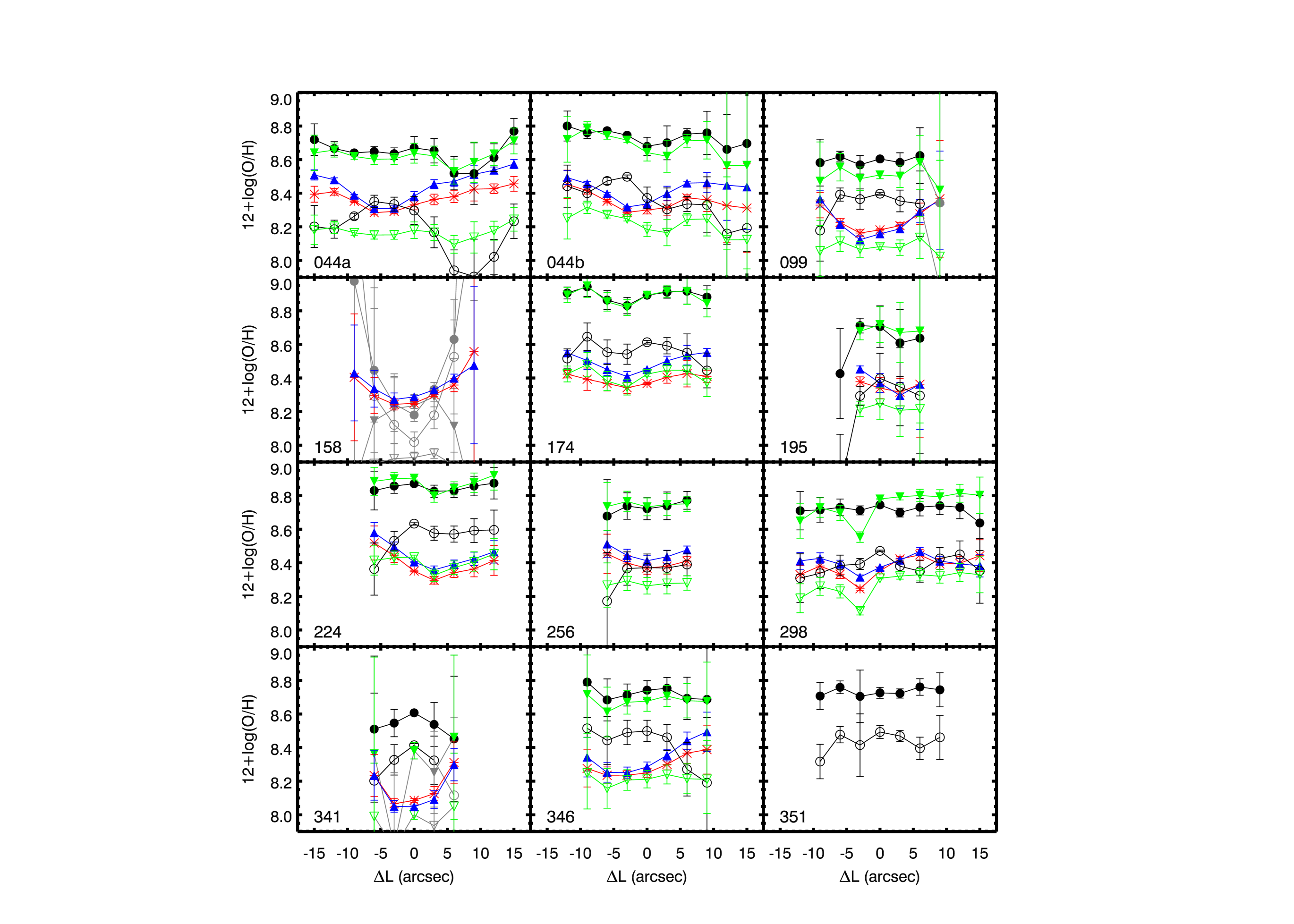
Figure 10.— Same diagrams with Figure 7 but the fluxes for the emission lines are corrected for the internal dust attenuation by adopting the Charlot & Fall (2000) curve of $\lambda^{-0.7}$.

Attenuation curves, depicting dust attenuation as a function of wavelength, are a necessary material for compensating dust attenuation and recovering intrinsic spectra in observational astrophysics. At present, attenuation curves have been found to be various in form. In this work, we apply the Fitzpatrick (1999) attenuation curve to the H ii regions observed in NGC 2403. The basic frame of this curve consists of three components parameterized with five coefficients (Fitzpatrick & Massa, 1988, 1990). This three-component parameterization has been tested to be feasible by a number of studies of the Milky Way (e.g., Whittet et al., 2004; Sofia et al., 2005; Gordon et al., 2009), the Magellanic Clouds (e.g., Gordon et al., 2003; Cartledge et al., 2005; Maíz Apellániz & Rubio, 2012), and galaxies from low to high redshifts (e.g., Rosa & Benvenuti, 1994; Zafar et al., 2012; Clayton et al., 2015). The Fitzpatrick (1999) curve is the specific parameterization by mean values for a number of sightlines in the Milky May, as is adopted in our work.

Another form of attenuation curves is provided by Cardelli et al. (1989), parameterized with $R_{\mathrm{V}}$ only, and widely used for Galactic extinction correction. We employed the Cardelli et al. (1989) curve for correcting Galactic extinction in this work. The Cardelli et al. (1989) curve is in agreement with the Fitzpatrick (1999) curve when $R_{\mathrm{V}}\sim 3.1$. However, the $R_{\mathrm{V}}$-dependent property for the attenuation curve has never been discovered in galaxies other than the Milky Way. Thus, application of the Cardelli et al. (1989) curve to extraGalactic environments is likely to render a mistake.

Through an investigation of galaxies as a whole, Calzetti et al. (2000) have obtained an attenuation curve expressed by a polynomial equation and exhibiting a smooth shape; a similarly featureless attenuation curve in a power-law form of $\lambda^{-0.7}$ has been produced with modeling by Charlot & Fall (2000). Both of the Calzetti et al. (2000) and Charlot & Fall (2000) curves are interpreted to be a statistical approximation of ”age-selective attenuation” which describes heavier dust obscuration for younger stellar populations (Granato et al., 2000; Panuzzo et al., 2007). Consequently, they are more suitable for statistic censuses of galaxies with integrated measurements. For studies of certain objects, these two curves appear to oversimplify the actual properties of dust obscuration.

In most cases, people are not able to ascertain an attenuation curve in a straightforward way but only presume one instead. The applicabilities of the attenuation curves presented above will help to make the choice in specific studies. In order to better illustrate respective characteristics of various attenuation curves, we perform a visual comparison by displaying seven typical attenuation curves, including the Fitzpatrick (1999) curve adopted in our work, the Cardelli et al. (1989) curve, the Calzetti et al. (2000) curve, the Charlot & Fall (2000) curve, and the curves for the Magellanic Clouds developed by Gordon et al. (2003), in Figure 9. As can be obviously seen, the most striking distinction of these attenuation curves lies in the wavelength range shorter than 2500 Å, which is due to differences in not only the slope of the curves but also the strength of the 2175 Å bump (see Mao et al., 2014, for elaborated influences of altering attenuation curves on UV-band observations). However, in the optical range, where our study is carried out, there is a high degree of consistency between all the curves except the Charlot & Fall (2000) one. In order to further inspect the influence of replacing the Fitzpatrick (1999) curve with the Charlot & Fall (2000) curve on the results, we replot the radial profiles of the oxygen abundances on the basis of the correction for internal dust attenuation with the Charlot & Fall (2000) curve in Figure 10, which shows that the change in the attenuation curve leads to very slight shifts for a few data points and does not affect our conclusions.

References

- Alloin et al. (1979) Alloin, D., Collin-Souffrin, S., Joly, M., & Vigroux, L. 1979, A&A, 78, 200
- Berg et al. (2013) Berg, D. A., Skillman, E. D., Garnett, D. R., et al. 2013, ApJ, 775, 128
- Bresolin (2007) Bresolin, F. 2007, ApJ, 656, 186
- Bresolin et al. (2009) Bresolin, F., Gieren, W., Kudritzki, R.-P., et al. 2009, ApJ, 700, 309
- Bresolin et al. (1999) Bresolin, F., Kennicutt, R. C., Jr., & Garnett, D. R. 1999, ApJ, 510, 104
- Calzetti (2001) Calzetti, D. 2001, PASP, 113, 1449
- Calzetti et al. (2000) Calzetti, D., Armus, L., Bohlin, R. C., et al. 2000, ApJ, 533, 682
- Cardelli et al. (1989) Cardelli, J. A., Clayton, G. C., & Mathis, J. S. 1989, ApJ, 345, 245
- Cartledge et al. (2005) Cartledge, S. I. B., Clayton, G. C., Gordon, K. D., et al. 2005, ApJ, 630, 355
- Castellanos et al. (2002) Castellanos, M., Díaz, A. I., & Terlevich, E. 2002, MNRAS, 329, 315
- Clayton et al. (2015) Clayton, G. C., Gordon, K. D., Bianchi, L. C., et al. 2015, ApJ, 815, 14
- Denicoló et al. (2002) Denicoló, G., Terlevich, R., & Terlevich, E. 2002, MNRAS, 330, 69
- Charlot & Fall (2000) Charlot, S., & Fall, S. M. 2000, ApJ, 539, 718
- Corbin & Warren (1991) Corbin, T. E., & Warren, W. H., Jr. 1991, International Reference Stars Catalog (Corbin 1991). Documentation for the machine-readable version., by Corbin, T. E.; Warren, W. H., Jr.. National Aeronautics and Space Administration (NASA), Greenbelt, MD (USA). National Space Science Data Center / World Data Center A for Rockets and Satellites, Apr 1991, 22 p.
- Dopita et al. (2000) Dopita, M. A., Kewley, L. J., Heisler, C. A., & Sutherland, R. S. 2000, ApJ, 542, 224
- Dopita et al. (2013) Dopita, M. A., Sutherland, R. S., Nicholls, D. C., Kewley, L. J., & Vogt, F. P. A. 2013, ApJS, 208, 10
- Drissen et al. (1999) Drissen, L., Roy, J.-R., Moffat, A. F. J., & Shara, M. M. 1999, AJ, 117, 1249
- Dutil & Roy (1999) Dutil, Y., & Roy, J.-R. 1999, ApJ, 516, 62
- Emerson (1996) Emerson, D. 1996, Interpreting Astronomical Spectra, by D. Emerson, pp. 472. John Wiley & Sons Ltd., June 1996., 187-251
- Fan et al. (2016) Fan, Z., Wang, H., Jiang, X., et al. 2016, PASP, 128, 115005
- Filippenko (1982) Filippenko, A. V. 1982, PASP, 94, 715
- Fitzpatrick (1999) Fitzpatrick, E. L. 1999, PASP, 111, 63
- Fitzpatrick & Massa (1988) Fitzpatrick, E. L., & Massa, D. 1988, ApJ, 328, 734
- Fitzpatrick & Massa (1990) Fitzpatrick, E. L., & Massa, D. 1990, ApJS, 72, 163
- Garnett (1992) Garnett, D. R. 1992, AJ, 103, 1330
- Garnett et al. (1999) Garnett, D. R., Shields, G. A., Peimbert, M., et al. 1999, ApJ, 513, 168
- Garnett et al. (1997) Garnett, D. R., Shields, G. A., Skillman, E. D., Sagan, S. P., & Dufour, R. J. 1997, ApJ, 489, 63
- Gordon et al. (2009) Gordon, K. D., Cartledge, S., & Clayton, G. C. 2009, ApJ, 705, 1320-1335
- Gordon et al. (2003) Gordon, K. D., Clayton, G. C., Misselt, K. A., Landolt, A. U., & Wolff, M. J. 2003, ApJ, 594, 279
- Granato et al. (2000) Granato, G. L., Lacey, C. G., Silva, L., et al. 2000, ApJ, 542, 710
- Hummer & Storey (1987) Hummer, D. G., & Storey, P. J. 1987, MNRAS, 224, 801
- Hodge & Kennicutt (1983) Hodge, P. W., & Kennicutt, R. C., Jr. 1983, AJ, 88, 296
- James et al. (2016) James, B. L., Auger, M., Aloisi, A., Calzetti, D., & Kewley, L. 2016, ApJ, 816, 40
- Kewley & Dopita (2002) Kewley, L. J., & Dopita, M. A. 2002, ApJS, 142, 35
- Kewley & Ellison (2008) Kewley, L. J., & Ellison, S. L. 2008, ApJ, 681, 1183
- Kennicutt et al. (2000) Kennicutt, R. C., Jr., Bresolin, F., French, H., & Martin, P. 2000, ApJ, 537, 589
- Kennicutt et al. (2003) Kennicutt, R. C., Jr., Bresolin, F., & Garnett, D. R. 2003, ApJ, 591, 801
- Kobulnicky et al. (1999) Kobulnicky, H. A., Kennicutt, R. C., Jr., & Pizagno, J. L. 1999, ApJ, 514, 544
- Kong et al. (2014) Kong, X., Lin, L., Li, J.-r., et al. 2014, Chinese Astron. Astrophys., 38, 427
- Liang et al. (2006) Liang, Y. C., Yin, S. Y., Hammer, F., et al. 2006, ApJ, 652, 257
- Mao et al. (2014) Mao, Y.-W., Kong, X., & Lin, L. 2014, ApJ, 789, 76
- Markwardt (2009) Markwardt, C. B. 2009, Astronomical Data Analysis Software and Systems XVIII, ASP Conference Series, 411, 251
- Maíz Apellániz & Rubio (2012) Maíz Apellániz, J., & Rubio, M. 2012, A&A, 541, A54
- McCall et al. (1985) McCall, M. L., Rybski, P. M., & Shields, G. A. 1985, ApJS, 57, 1
- McGaugh (1991) McGaugh, S. S. 1991, ApJ, 380, 140
- Monreal-Ibero et al. (2011) Monreal-Ibero, A., Relaño, M., Kehrig, C., et al. 2011, MNRAS, 413, 2242
- Moustakas et al. (2010) Moustakas, J., Kennicutt, R. C., Jr., Tremonti, C. A., Dale, D. A., Smith, J.-D. T., & Calzetti, D. 2010, ApJS, 190, 233
- Oey & Shields (2000) Oey, M. S., & Shields, J. C. 2000, ApJ, 539, 687
- Osterbrock & Ferland (2006) Osterbrock, D. E., & Ferland, G. J. 2006, Astrophysics of gaseous nebulae and active galactic nuclei, 2nd. ed. by D.E. Osterbrock and G.J. Ferland. Sausalito, CA: University Science Books, 2006, 67-106
- Panuzzo et al. (2007) Panuzzo, P., Granato, G. L., Buat, V., et al. 2007, MNRAS, 375, 640
- Pagel et al. (1979) Pagel, B. E. J., Edmunds, M. G., Blackwell, D. E., Chun, M. S., & Smith, G. 1979, MNRAS, 189, 95
- Pellegrini et al. (2012) Pellegrini, E. W., Oey, M. S., Winkler, P. F., et al. 2012, ApJ, 755, 40
- Pérez-Montero (2017) Pérez-Montero, E. 2017, PASP, 129, 043001
- Pérez-Montero et al. (2014) Pérez-Montero, E., Monreal-Ibero, A., Relaño, M., et al. 2014, A&A, 566, A12
- Pérez-Montero et al. (2011) Pérez-Montero, E., Relaño, M., Vílchez, J. M., & Monreal-Ibero, A. 2011, MNRAS, 412, 675
- Pettini & Pagel (2004) Pettini, M., & Pagel, B. E. J. 2004, MNRAS, 348, L59
- Pilyugin & Grebel (2016) Pilyugin, L. S., & Grebel, E. K. 2016, MNRAS, 457, 3678
- Pilyugin & Thuan (2005) Pilyugin, L. S., & Thuan, T. X. 2005, ApJ, 631, 231
- Pilyugin et al. (2010) Pilyugin, L. S., Vílchez, J. M., & Thuan, T. X. 2010, ApJ, 720, 1738
- Relaño et al. (2010) Relaño, M., Monreal-Ibero, A., Vílchez, J. M., & Kennicutt, R. C. 2010, MNRAS, 402, 1635
- Rosa & Benvenuti (1994) Rosa, M. R., & Benvenuti, P. 1994, A&A, 291, 1
- Schlegel et al. (1998) Schlegel, D. J., Finkbeiner, D. P., & Davis, M. 1998, ApJ, 500, 525
- Sivan et al. (1990) Sivan, J.-P., Maucherat, A. J., Petit, H., & Comte, G. 1990, A&A, 237, 23
- Skillman & Kennicutt (1993) Skillman, E. D., & Kennicutt, R. C., Jr. 1993, ApJ, 411, 655
- Sofia et al. (2005) Sofia, U. J., Wolff, M. J., Rachford, B., et al. 2005, ApJ, 625, 167
- van Zee et al. (1998) van Zee, L., Salzer, J. J., Haynes, M. P., O’Donoghue, A. A., & Balonek, T. J. 1998, AJ, 116, 2805
- Vinkó et al. (2006) Vinkó, J., Takáts, K., Sárneczky, K., et al. 2006, MNRAS, 369, 1780
- Whittet et al. (2004) Whittet, D. C. B., Shenoy, S. S., Clayton, G. C., & Gordon, K. D. 2004, ApJ, 602, 291
- Zafar et al. (2012) Zafar, T., Watson, D., Elíasdóttir, Á., et al. 2012, ApJ, 753, 82
- Zahid et al. (2012) Zahid, H. J., Bresolin, F., Kewley, L. J., Coil, A. L., & Davé, R. 2012, ApJ, 750, 120