Super-Resolution mmWave Channel Estimation using Atomic Norm Minimization

Hongyun Chu,  Le Zheng,  and Xiaodong Wang H. Chu is with the Wireless Energy and Information Transmission Lab, Shenzhen Institutes of Advanced Technology, Chinese Academy of Sciences, Shenzhen, 518055, China.L. Zheng and X. Wang are with the Electrical Engineering Department, Columbia University, New York 10027, USA, e-mail: le.zheng.cn@gmail.com; wangx@ee.columbia.edu.
Abstract

We propose super-resolution MIMO channel estimators for millimeter-wave (mmWave) systems that employ hybrid analog and digital beamforming and generalized spatial modulation, respectively. Exploiting the inherent sparsity of mmWave channels, the channel estimation problem is formulated as an atomic norm minimization that enhances sparsity in the continuous angles of departure and arrival. Both pilot-assisted and data-aided channel estimators are developed, with the former one formulated as a convex problem and the latter as a non-convex problem. To solve these formulated channel estimation problems, we develop a computationally efficient conjugate gradient descent method based on non-convex factorization which restricts the search space to low-rank matrices. Simulation results are presented to illustrate the superior channel estimation performance of the proposed algorithms for both types of mmWave systems compared to the existing compressed-sensing-based estimators with finely quantized angle grids.

Index Terms:
Millimeter-wave, channel estimation, hybrid beamforming, generalized spatial modulation, atomic norm minimization, sparsity, conjugate gradient descent, non-convex factorization.

I Introduction

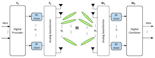
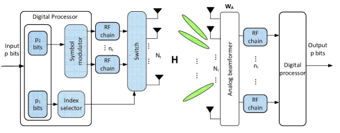
The millimeter-wave (mmWave) spectrum band has been made available for future 5G wireless communication systems [1]. To compensate for the severe signal propagation loss at mmWave band and to achieve data rates on the order of gigabits per second, the mmWave systems are expected to employ large antenna arrays at transceivers to provide sufficient beamforming gains. However, due to the high cost of mmWave radio frequency (RF) units, it is infeasible to associate an RF chain with each antenna element in such large mmWave MIMO systems in practice. Two large MIMO architectures have been proposed for mmWave systems that employ a much smaller number of RF chains than the number of antennas at the transceivers. One is the hybrid beamforming (HB) system [2, 12], shown in Fig. 1(a), that employs a cascade of analog and digital beamformers at both the transmitter and receiver. The other is the generalized spatial modulation (GSM) system [3], shown in Fig. 1(b), that only activates antennas that are linked to RF chains. Note that in the HB system information bits are carried on the transmitted modulation symbols, whereas in the GSM system information bits are conveyed by both the index set of the activated transmit antennas and the transmitted modulation symbols. It is well known that in MIMO systems the channel state information (CSI) is indispensable for reliable signal transmission and reception, and especially useful for designing efficient beamformers in mmWave band [18]. However, channel estimation is challenging for mmWave systems with a large number of antennas, and conventional channel estimation methods based on the rich scattering assumption developed for microwave systems are rather inefficient due to high training overhead and high computational cost.

In [5], it is pointed out that the parametric channel model for mmWave systems leads to a sparse representation of the MIMO channel, which can be exploited for channel estimation purpose - i.e., instead of estimating the full channel matrix, one would estimate only the angles of departure/arrival (AoD/AoA) of dominant paths and the corresponding path gains. Leveraging on this, various channel estimators have been proposed in [4, 5, 6, 7, 8, 9, 10, 11, 12] that capitalize on the spatial sparsity of mmWave channels. In particular, in [4, 5], closed-loop beam training based methods such as multistage beam search are proposed for channel estimation. While such closed-loop methods have been adopted in practical systems, their performance tends to be limited by the training beam patterns.

As an alternative to the closed-loop based beam training techniques, the open-loop techniques perform explicit channel estimation using MUSIC and compressive sensing (CS) methods, by transmitting pilot symbols. In [6], a subspace-based mmWave channel estimation method that makes use of the MUSIC algorithm is proposed. A two-dimensional (2D) MUSIC algorithm for beamformed mmWave MIMO channel estimation is proposed in [7]. The MUSIC algorithm is able to identify multiple paths with high resolution but it is sensitive to antenna position, gain, and phase error. On the other hand, a number of CS-based channel estimators [8, 9, 12, 10, 11] have been proposed based on the virtual angular domain representation of MIMO channels [10, 11], which describes the channel with respect to some fixed basis functions of angles whose resolution is determined by the spatial resolution of arrays.

Different from the traditional grid-based CS techniques, a gridless approach, which uses atomic norm minimization to manifest the signal sparsity in the continuous parameter domain, has been proposed for several signal processing applications [13]. Under certain conditions, atomic norm minimization can achieve exact sparse signals reconstruction, avoiding the effects of basis mismatch which can plague grid-based CS techniques.

In this paper, we propose super-resolution mmWave channel estimators based on atomic norm minimization for both the HB system and GSM system. First, the pilot-assisted channel estimator is formulated as a convex optimization problem under the atomic norm minimization framework that exploits the sparsity in the continuous AoD/AoA domains. Then to account for the slowly time-varying nature of the block-fading channels, the data-aided channel estimator is formulated as a combined atomic norm and 1subscript1\ell_{1}-norm minimization problem, which is non-convex. Here the 1subscript1\ell_{1}-norm is to exploit the sparsity in the demodulation errors. Moreover, we develop computationally efficient non-convex methods to solve both channel estimation formulations based on non-convex factorization and conjugate gradient descent (CGD). Extensive simulation results are provided to illustrate the superior performance of the proposed new channel estimators compared with the existing CS-based methods.

The remainder of this paper is organized as follows. Section II describes the mmWave channel model and the signal models for both the HB system and GSM system. Section III gives the formulations of both pilot-assisted and data-aided channel estimators. Section IV presents the proposed non-convex method for solving both channel estimation formulations. Simulation results are given in Section V. Finally, Section VI concludes the paper.

II System Descriptions

In this section, we first present the mmWave channel model and then the signal models for the HB system and GSM system, respectively.

II-A Channel Model

We consider a wireless communication system operating at mmWave band. The transmitter has Ntsubscript𝑁𝑡N_{t} antennas and ntsubscript𝑛𝑡n_{t} RF chains, and the receiver has Nrsubscript𝑁𝑟N_{r} antennas and nrsubscript𝑛𝑟n_{r} RF chains, where max(nt,nr)subscript𝑛𝑡subscript𝑛𝑟absent(n_{t},n_{r})\leq min(Nt,Nr)subscript𝑁𝑡subscript𝑁𝑟(N_{t},N_{r}). Both the transmit and receive antennas are uniform linear arrays.

We assume a geometric MIMO channel model [14] that has L𝐿L scatterers during a time block. Thus, the channel matrix in a time block can be expressed as

𝐇=l=1Lαl𝐚R(ϕl)𝐚TH(θl)Nr×Nt,𝐇superscriptsubscript𝑙1𝐿subscript𝛼𝑙subscript𝐚𝑅subscriptitalic-ϕ𝑙superscriptsubscript𝐚𝑇𝐻subscript𝜃𝑙superscriptsubscript𝑁𝑟subscript𝑁𝑡\displaystyle\mathbf{H}=\sum\limits_{l=1}^{L}{\alpha_{l}}\mathbf{a}_{R}(\phi_{l})\mathbf{a}_{T}^{H}(\theta_{l})\in\mathbb{C}^{N_{r}\times N_{t}}, (1)

where αl𝒞𝒩(0,σl2)similar-tosubscript𝛼𝑙𝒞𝒩0superscriptsubscript𝜎𝑙2\alpha_{l}\sim\mathcal{CN}(0,\sigma_{l}^{2}) is the complex gain of the l𝑙l-th path, σl2superscriptsubscript𝜎𝑙2\sigma_{l}^{2} is the average power gain of the l𝑙l-th path. Assuming that the antenna arrays are installed in the horizontal direction, we denote ϕl=sin(ϕ¯l)[0,1)subscriptitalic-ϕ𝑙subscript¯italic-ϕ𝑙01\phi_{l}=\sin(\bar{\phi}_{l})\in[0,1) and θl=sin(θ¯l)[0,1)subscript𝜃𝑙subscript¯𝜃𝑙01\theta_{l}=\sin(\bar{\theta}_{l})\in[0,1) as the departure and arrival directions of the l𝑙l-th path, respectively, where ϕ¯lsubscript¯italic-ϕ𝑙\bar{\phi}_{l} and θ¯lsubscript¯𝜃𝑙\bar{\theta}_{l} are the physical azimuth angles of departure and arrival (AoD/AoA), respectively. 𝐚T(θl)subscript𝐚𝑇subscript𝜃𝑙{\mathbf{a}_{T}}(\theta_{l}) represents the normalized transmit array response vector at the direction of θlsubscript𝜃𝑙\theta_{l} given by

𝐚T(θl)=1Nt[1,ej2πλdθl,,ej(Nt1)2πλdθl]TNt×1,subscript𝐚𝑇subscript𝜃𝑙1subscript𝑁𝑡superscript1superscript𝑒𝑗2𝜋𝜆𝑑subscript𝜃𝑙superscript𝑒𝑗subscript𝑁𝑡12𝜋𝜆𝑑subscript𝜃𝑙𝑇superscriptsubscript𝑁𝑡1\mathbf{a}_{T}(\theta_{l})=\frac{1}{\sqrt{N_{t}}}{\left[{1,{e^{j\frac{2\pi}{\lambda}d\theta_{l}}},...,{e^{j(N_{t}-1)\frac{{2\pi}}{\lambda}d\theta_{l}}}}\right]^{T}}\in\mathbb{C}^{N_{t}\times 1}, (2)

where λ𝜆\lambda is the wavelength, d𝑑d is the inter-antenna element spacing with dλ/2𝑑𝜆2d\geq\lambda/2. The antenna array response 𝐚R(ϕl)subscript𝐚𝑅subscriptitalic-ϕ𝑙\mathbf{a}_{R}(\phi_{l}) at the receiver can be written similarly.

Thus, (1) can be expressed compactly as

𝐇=𝐀R𝚲𝐀THNr×Nt,𝐇subscript𝐀𝑅𝚲superscriptsubscript𝐀𝑇𝐻superscriptsubscript𝑁𝑟subscript𝑁𝑡\mathbf{H}=\mathbf{A}_{R}\mathbf{\Lambda}\mathbf{A}_{T}^{H}\in\mathbb{C}^{N_{r}\times N_{t}}, (3)

where 𝚲=diag([α1,α2,,αL]T)𝚲diagsuperscriptsubscript𝛼1subscript𝛼2subscript𝛼𝐿𝑇\mathbf{\Lambda}=\mathrm{diag}([\alpha_{1},\alpha_{2},...,\alpha_{L}]^{T}), and

𝐀Tsubscript𝐀𝑇\displaystyle\mathbf{A}_{T} =\displaystyle= [𝐚T(θ1),,𝐚T(θL)]Nt×L,subscript𝐚𝑇subscript𝜃1subscript𝐚𝑇subscript𝜃𝐿superscriptsubscript𝑁𝑡𝐿\displaystyle[\mathbf{a}_{T}(\theta_{1}),...,\mathbf{a}_{T}(\theta_{L})]\in\mathbb{C}^{N_{t}\times L}, (4)
𝐀Rsubscript𝐀𝑅\displaystyle\mathbf{A}_{R} =\displaystyle= [𝐚R(ϕ1),,𝐚R(ϕL)]Nr×L.subscript𝐚𝑅subscriptitalic-ϕ1subscript𝐚𝑅subscriptitalic-ϕ𝐿superscriptsubscript𝑁𝑟𝐿\displaystyle[\mathbf{a}_{R}(\phi_{1}),...,\mathbf{a}_{R}(\phi_{L})]\in\mathbb{C}^{N_{r}\times L}. (5)

II-B Signal Models

In this paper, we will consider both the HB system and GSM system illustrated in Fig. 1(a) and Fig. 1(b), respectively.
Refer to caption
(a) The HB system.
Refer to caption
(b) The GSM system.
Figure 1: The HB system and GSM system.

For both systems, the transmitted signal during the k𝑘k-th time slot is denoted by 𝐱kNt×1,k=1,2,,Kformulae-sequencesubscript𝐱𝑘superscriptsubscript𝑁𝑡1𝑘12𝐾\mathbf{x}_{k}\in\mathbb{C}^{N_{t}\times 1},k=1,2,...,K. The Nrsubscript𝑁𝑟N_{r}-dimensional signal at the receive antenna array is processed by a linear filter 𝐖Nr×nr𝐖superscriptsubscript𝑁𝑟subscript𝑛𝑟\mathbf{W}\in\mathbb{C}^{N_{r}\times n_{r}}, resulting in the following signal at the output of the receive RF chain

𝐲k=𝐖H𝐇𝐱k+𝐖H𝐧knr×1,subscript𝐲𝑘superscript𝐖𝐻subscript𝐇𝐱𝑘superscript𝐖𝐻subscript𝐧𝑘superscriptsubscript𝑛𝑟1\mathbf{y}_{k}=\mathbf{W}^{H}\mathbf{H}\mathbf{x}_{k}+\mathbf{W}^{H}\mathbf{n}_{k}\in\mathbb{C}^{{n_{r}}\times 1}, (6)

where 𝐧k𝒞𝒩(0,σ2𝐈Nr)Nr×1similar-tosubscript𝐧𝑘𝒞𝒩0superscript𝜎2subscript𝐈subscript𝑁𝑟superscriptsubscript𝑁𝑟1\mathbf{n}_{k}\sim\mathcal{CN}(0,\sigma^{2}\mathbf{I}_{N_{r}})\in\mathbb{C}^{N_{r}\times 1} is the additive white Gaussian noise and 𝐈Nrsubscript𝐈subscript𝑁𝑟\mathbf{I}_{N_{r}} denotes a Nr×Nrsubscript𝑁𝑟subscript𝑁𝑟N_{r}\times N_{r} identity matrix. Denoting 𝐗=[𝐱1,𝐱2,,𝐱K]𝐗subscript𝐱1subscript𝐱2subscript𝐱𝐾\mathbf{X}=[\mathbf{x}_{1},\mathbf{x}_{2},...,\mathbf{x}_{K}], 𝐘=[𝐲1,𝐲2,,𝐲K]𝐘subscript𝐲1subscript𝐲2subscript𝐲𝐾\mathbf{Y}=[\mathbf{y}_{1},\mathbf{y}_{2},...,\mathbf{y}_{K}] and 𝐐=𝐖H[𝐧1,𝐧2,,𝐧K]𝐐superscript𝐖𝐻subscript𝐧1subscript𝐧2subscript𝐧𝐾\mathbf{Q}=\mathbf{W}^{H}[\mathbf{n}_{1},\mathbf{n}_{2},...,\mathbf{n}_{K}], then (5) can be written as

𝐘=𝐖H𝐇𝐗+𝐐.𝐘superscript𝐖𝐻𝐇𝐗𝐐\mathbf{Y}=\mathbf{W}^{H}\mathbf{H}\mathbf{X}+\mathbf{Q}. (7)

II-B1 HB System

In the HB system, the transmitted signal is given by 𝐱k=𝐅𝐬k=𝐅A𝐅D𝐬ksubscript𝐱𝑘subscript𝐅𝐬𝑘subscript𝐅𝐴subscript𝐅𝐷subscript𝐬𝑘\mathbf{x}_{k}=\mathbf{F}\mathbf{s}_{k}=\mathbf{F}_{A}\mathbf{F}_{D}\mathbf{s}_{k}, where 𝐬kMssubscript𝐬𝑘superscriptsubscript𝑀𝑠\mathbf{s}_{k}\in{\cal M}^{M_{s}} is the data symbol vector, with {\cal M} being the symbol constellation set, Msntsubscript𝑀𝑠subscript𝑛𝑡M_{s}\leq n_{t} is the number of data streams, 𝐅Dnt×Mssubscript𝐅𝐷superscriptsubscript𝑛𝑡subscript𝑀𝑠\mathbf{F}_{D}\in\mathbb{C}^{n_{t}\times M_{s}} is the digital precoder that adjusts both amplitudes and phases, and 𝐅ANt×ntsubscript𝐅𝐴superscriptsubscript𝑁𝑡subscript𝑛𝑡\mathbf{F}_{A}\in\mathbb{C}^{N_{t}\times n_{t}} is the analog RF precoder that only adjusts phases. At the receiver, the received signal is firstly passed through the analog RF combiner 𝐖ANr×nrsubscript𝐖𝐴superscriptsubscript𝑁𝑟subscript𝑛𝑟\mathbf{W}_{A}\in\mathbb{C}^{N_{r}\times n_{r}} and then the baseband combiner 𝐖Dnr×Mssubscript𝐖𝐷superscriptsubscript𝑛𝑟subscript𝑀𝑠\mathbf{W}_{D}\in\mathbb{C}^{n_{r}\times M_{s}}. Hence the combiner 𝐖𝐖\mathbf{W} in (6) can be written as 𝐖=𝐖A𝐖D𝐖subscript𝐖𝐴subscript𝐖𝐷\mathbf{W}=\mathbf{W}_{A}\mathbf{W}_{D}. Note that all elements of 𝐅Asubscript𝐅𝐴\mathbf{F}_{A} and 𝐖Asubscript𝐖𝐴\mathbf{W}_{A} should have constant amplitudes. Examples of the analog filters 𝐅Asubscript𝐅𝐴\mathbf{F}_{A}, 𝐖Asubscript𝐖𝐴\mathbf{W}_{A}, and digital filters 𝐅Dsubscript𝐅𝐷\mathbf{F}_{D}, 𝐖Dsubscript𝐖𝐷\mathbf{W}_{D} can be found in [18].

In particular, during the pilot training stage, we set Ms=nt=nrsubscript𝑀𝑠subscript𝑛𝑡subscript𝑛𝑟M_{s}=n_{t}=n_{r} and the digital filters 𝐅D=𝐈ntsubscript𝐅𝐷subscript𝐈subscript𝑛𝑡\mathbf{F}_{D}=\mathbf{I}_{n_{t}}, 𝐖D=𝐈nrsubscript𝐖𝐷subscript𝐈subscript𝑛𝑟\mathbf{W}_{D}=\mathbf{I}_{n_{r}}. The DFT beamformers can be employed as the analog filters, given by

𝐅Asubscript𝐅𝐴\displaystyle\mathbf{F}_{A} =\displaystyle= [𝐚T(θ¯1),,𝐚T(θ¯nt)]Nt×nt,subscript𝐚𝑇subscript¯𝜃1subscript𝐚𝑇subscript¯𝜃subscript𝑛𝑡superscriptsubscript𝑁𝑡subscript𝑛𝑡\displaystyle[\mathbf{a}_{T}(\bar{\theta}_{1}),...,\mathbf{a}_{T}(\bar{\theta}_{n_{t}})]\in\mathbb{C}^{N_{t}\times n_{t}}, (8)
𝐖Asubscript𝐖𝐴\displaystyle\mathbf{W}_{A} =\displaystyle= [𝐚R(ϕ¯1),,𝐚R(ϕ¯nr)]Nr×nr,subscript𝐚𝑅subscript¯italic-ϕ1subscript𝐚𝑅subscript¯italic-ϕsubscript𝑛𝑟superscriptsubscript𝑁𝑟subscript𝑛𝑟\displaystyle[\mathbf{a}_{R}(\bar{\phi}_{1}),...,\mathbf{a}_{R}(\bar{\phi}_{n_{r}})]\in\mathbb{C}^{N_{r}\times n_{r}}, (9)

where

θ¯isubscript¯𝜃𝑖\displaystyle\bar{\theta}_{i} =\displaystyle= θ¯1+2Nt(i1),i=1,2,,nt,formulae-sequencesubscript¯𝜃12subscript𝑁𝑡𝑖1𝑖12subscript𝑛𝑡\displaystyle\bar{\theta}_{1}+\frac{2}{N_{t}}(i-1),~{}~{}i=1,2,...,n_{t}, (10)
ϕ¯jsubscript¯italic-ϕ𝑗\displaystyle\bar{\phi}_{j} =\displaystyle= ϕ¯1+2Nr(j1),j=1,2,,nr,formulae-sequencesubscript¯italic-ϕ12subscript𝑁𝑟𝑗1𝑗12subscript𝑛𝑟\displaystyle\bar{\phi}_{1}+\frac{2}{N_{r}}(j-1),j=1,2,...,n_{r}, (11)

with θ¯isubscript¯𝜃𝑖\bar{\theta}_{i}, ϕ¯j[0,1)subscript¯italic-ϕ𝑗01\bar{\phi}_{j}\in[0,1) denoting the pointing directions of the i𝑖i-th transmit beam and the j𝑗j-th receive beam, respectively.

II-B2 GSM System

In the GSM system, in each time slot, only ntsubscript𝑛𝑡n_{t} out of Ntsubscript𝑁𝑡N_{t} transmit antennas are activated to transmit data while the other Ntntsubscript𝑁𝑡subscript𝑛𝑡N_{t}-n_{t} transmit antennas remain idle. The information bits are conveyed by not only the modulation symbols but also the indices of the active antennas. As shown in Fig. 1(b), at the transmitter, a block of p=p1+p2𝑝subscript𝑝1subscript𝑝2p=p_{1}+p_{2} information bits is divided into two parts. The first p1=log2(Ntnt)subscript𝑝1subscript2binomialsubscript𝑁𝑡subscript𝑛𝑡p_{1}=\lfloor\log_{2}{N_{t}\choose n_{t}}\rfloor bits are fed to the index selector to determine the indices of ntsubscript𝑛𝑡n_{t} active antennas 𝒰𝒰\cal{U}={u1,u2,,unt}absentsubscript𝑢1subscript𝑢2subscript𝑢subscript𝑛𝑡=\{u_{1},u_{2},...,u_{n_{t}}\}, where um{1,2,,Nt}subscript𝑢𝑚12subscript𝑁𝑡u_{m}\in\{1,2,...,N_{t}\} for m=1,2,,nt𝑚12subscript𝑛𝑡m=1,2,...,n_{t} and u1<u2<<untsubscript𝑢1subscript𝑢2subscript𝑢subscript𝑛𝑡u_{1}<u_{2}<...<u_{n_{t}}. Note that among (Ntnt)binomialsubscript𝑁𝑡subscript𝑛𝑡N_{t}\choose n_{t} possible transmit antenna combinations, only 2p1superscript2subscript𝑝12^{p_{1}} transmit antenna combinations are permitted and the other (Ntnt2p1)binomialsubscript𝑁𝑡subscript𝑛𝑡superscript2subscript𝑝1N_{t}\choose n_{t}-2^{p_{1}} combinations are illegal. The remaining p2=ntlog2Msubscript𝑝2subscript𝑛𝑡subscript2𝑀p_{2}=n_{t}\log_{2}M bits are then fed to the symbol modulator to generate ntsubscript𝑛𝑡n_{t} modulation symbols each drawn from a constellation alphabet \cal M of cardinality M𝑀M and carried on an antenna indexed by an element in 𝒰𝒰\cal U, resulting in the transmitted signal 𝐱k=[xk(1),xk(2),,xk(Nt)]Tsubscript𝐱𝑘superscriptsubscript𝑥𝑘1subscript𝑥𝑘2subscript𝑥𝑘subscript𝑁𝑡𝑇\mathbf{x}_{k}=[x_{k}(1),x_{k}(2),...,x_{k}(N_{t})]^{T} in (6)-(7), where

xk(n)={sm,n=um𝒰,0,n𝒰,n=1,2,,Nt.\displaystyle{{x}_{k}}(n)=\left\{\begin{gathered}{s_{m}}\in{\cal M},~{}n={u_{m}}\in\cal U,\hfill\\ 0,~{}~{}~{}~{}~{}~{}~{}~{}~{}~{}n\notin\cal U,\hfill\end{gathered}\right.\quad n=1,2,\ldots,N_{t}. (14)

Hence xk(n){0}subscript𝑥𝑘𝑛0x_{k}(n)\in{{\cal M}\cup\{0\}} and 𝐱k0=ntsubscriptnormsubscript𝐱𝑘0subscript𝑛𝑡\|\mathbf{x}_{k}\|_{0}=n_{t}. The mapping of p1subscript𝑝1p_{1} bits for index selection can be implemented by using a look-up table or the combinatorial method [21]. In the signal model (6)-(7), for the GSM system, we have 𝐖=𝐖ANr×nr𝐖subscript𝐖𝐴superscriptsubscript𝑁𝑟subscript𝑛𝑟\mathbf{W}=\mathbf{W}_{A}\in{\mathbb{C}}^{N_{r}\times n_{r}}. For example, the DFT beamformers in (8)-(9) can be employed.

III Channel Estimation Based on Atomic Norm Minimization

In this section, we formulate the mmWave channel estimation problem as an atomic norm based sparse recovery problem in the continuous AoD/AoA domains. Both the pilot-assisted and data-aided channel estimators are developed.

From (1), estimating the channel matrix 𝐇𝐇\mathbf{H} is equivalent to estimating the parameters of the L𝐿L paths, i.e., {αl,ϕl,θl}l=1L.superscriptsubscriptsubscript𝛼𝑙subscriptitalic-ϕ𝑙subscript𝜃𝑙𝑙1𝐿\{\alpha_{l},\phi_{l},\theta_{l}\}_{l=1}^{L}. Since the number of scatters L𝐿L in the mmWave channel is typically small, the system exhibits sparsity that can be exploited for channel estimation purpose. To begin with, we vectorize 𝐘𝐘\mathbf{Y} in (7) to obtain

𝐲~=vec(𝐘)=(𝐗T𝐖H)𝐡~+𝐪~=(𝐗T𝐖H)(𝐀T𝐀R)𝜶+𝐪~,~𝐲vec𝐘tensor-productsuperscript𝐗𝑇superscript𝐖𝐻~𝐡~𝐪tensor-productsuperscript𝐗𝑇superscript𝐖𝐻direct-productsubscriptsuperscript𝐀𝑇subscript𝐀𝑅𝜶~𝐪\tilde{\mathbf{y}}=\mathrm{vec}(\mathbf{Y})=(\mathbf{X}^{T}\otimes\mathbf{W}^{H})\mathbf{\tilde{h}}+\mathbf{\tilde{q}}=(\mathbf{X}^{T}\otimes\mathbf{W}^{H})(\mathbf{A}^{\ast}_{T}\odot\mathbf{A}_{R})\bm{\alpha}+\mathbf{\tilde{q}}, (15)

where 𝜶=[α1,α2,,αL]T𝜶superscriptsubscript𝛼1subscript𝛼2subscript𝛼𝐿𝑇\bm{\alpha}=[\alpha_{1},\alpha_{2},...,\alpha_{L}]^{T}, 𝐗T𝐖HnrK×NtNrtensor-productsuperscript𝐗𝑇superscript𝐖𝐻superscriptsubscript𝑛𝑟𝐾subscript𝑁𝑡subscript𝑁𝑟\mathbf{X}^{T}\otimes\mathbf{W}^{H}\in\mathbb{C}^{n_{r}K\times{N_{t}N_{r}}} with tensor-product\otimes being the Kronecker product, 𝐡~=vec(𝐇)NtNr×1~𝐡vec𝐇superscriptsubscript𝑁𝑡subscript𝑁𝑟1\tilde{\mathbf{h}}=\mathrm{vec}(\mathbf{H})\in\mathbb{C}^{N_{t}N_{r}\times 1} and 𝐪~=vec(𝐐)NtNr×1~𝐪vec𝐐superscriptsubscript𝑁𝑡subscript𝑁𝑟1\mathbf{\tilde{q}}=\mathrm{vec}(\mathbf{Q})\in\mathbb{C}^{N_{t}N_{r}\times 1}. 𝐀T𝐀Rdirect-productsubscriptsuperscript𝐀𝑇subscript𝐀𝑅\mathbf{A}^{\ast}_{T}\odot\mathbf{A}_{R} is an NtNr×Lsubscript𝑁𝑡subscript𝑁𝑟𝐿N_{t}N_{r}\times L matrix in which each column has the form 𝐚T(θl)𝐚R(ϕl)tensor-productsubscriptsuperscript𝐚𝑇subscript𝜃𝑙subscript𝐚𝑅subscriptitalic-ϕ𝑙\mathbf{a}^{\ast}_{T}(\theta_{l})\otimes\mathbf{a}_{R}(\phi_{l}), with \ast being the conjugation operation and direct-product\odot being the Khatri-Rao product.

III-A Channel Estimation Based on On-grid CS Algorithm

Before describing our proposed mmWave channel estimators, we briefly discuss some existing CS-based mmWave channel estimation methods [12]. Estimating 𝐇𝐇\mathbf{H} is equivalent to jointly estimating the unknown parameters 𝜶𝜶\bm{\alpha}, 𝐀Tsubscript𝐀𝑇\mathbf{A}_{T} and 𝐀Rsubscript𝐀𝑅\mathbf{A}_{R} from the noisy observations 𝐲~~𝐲\tilde{\mathbf{y}} in (15), which is a non-linear problem. However, it can be linearized by using an overcomplete dictionary matrix defined as 𝐀~T𝐀~Rdirect-productsuperscriptsubscript~𝐀𝑇subscript~𝐀𝑅\mathbf{\tilde{A}}_{T}^{\ast}\odot\mathbf{\tilde{A}}_{R} [22] with

𝐀~Tsubscript~𝐀𝑇\displaystyle\mathbf{\tilde{A}}_{T} =\displaystyle= [𝐚T(θ~1),𝐚T(θ~2),,𝐚T(θ~J~)]Nt×J~,subscript𝐚𝑇superscriptsubscript~𝜃1subscript𝐚𝑇superscriptsubscript~𝜃2subscript𝐚𝑇superscriptsubscript~𝜃~𝐽superscriptsubscript𝑁𝑡~𝐽\displaystyle[\mathbf{a}_{T}(\tilde{\theta}_{1}^{\prime}),\mathbf{a}_{T}(\tilde{\theta}_{2}^{\prime}),...,\mathbf{a}_{T}(\tilde{\theta}_{\tilde{J}}^{\prime})]\in\mathbb{C}^{N_{t}\times\tilde{J}}, (16)
𝐀~Rsubscript~𝐀𝑅\displaystyle\mathbf{\tilde{A}}_{R} =\displaystyle= [𝐚R(ϕ~1),𝐚R(ϕ~2),,𝐚R(ϕ~J~)]Nr×J~,subscript𝐚𝑅superscriptsubscript~italic-ϕ1subscript𝐚𝑅superscriptsubscript~italic-ϕ2subscript𝐚𝑅superscriptsubscript~italic-ϕ~𝐽superscriptsubscript𝑁𝑟~𝐽\displaystyle[\mathbf{a}_{R}(\tilde{\phi}_{1}^{\prime}),\mathbf{a}_{R}(\tilde{\phi}_{2}^{\prime}),...,\mathbf{a}_{R}(\tilde{\phi}_{\tilde{J}}^{\prime})]\in\mathbb{C}^{N_{r}\times\tilde{J}}, (17)

where {θ~j}j=1J~superscriptsubscriptsuperscriptsubscript~𝜃𝑗𝑗1~𝐽\{\tilde{\theta}_{j}^{\prime}\}_{j=1}^{\tilde{J}} and {ϕ~j}j=1J~superscriptsubscriptsuperscriptsubscript~italic-ϕ𝑗𝑗1~𝐽\{\tilde{\phi}_{j}^{\prime}\}_{j=1}^{\tilde{J}} denote sets of uniformly spaced points in the interval [0,1)01[0,1), and J~~𝐽\tilde{J} is the number of columns of 𝐀~Tsubscript~𝐀𝑇\mathbf{\tilde{A}}_{T} or 𝐀~Rsubscript~𝐀𝑅\mathbf{\tilde{A}}_{R} where J~Lmuch-greater-than~𝐽𝐿\tilde{J}\gg L. For sufficiently large J~~𝐽\tilde{J}, the angles are densely sampled. Let 𝜶~=[α~1,α~2,,α~J~]TJ~×1~𝜶superscriptsuperscriptsubscript~𝛼1superscriptsubscript~𝛼2superscriptsubscript~𝛼~𝐽𝑇superscript~𝐽1\tilde{\bm{\alpha}}=[\tilde{\alpha}_{1}^{\prime},\tilde{\alpha}_{2}^{\prime},...,\tilde{\alpha}_{\tilde{J}}^{\prime}]^{T}\in\mathbb{C}^{\tilde{J}\times 1} be the sparse vector whose non-zero elements correspond to 𝜶𝜶\bm{\alpha} in (15). Thus, the non-linear parameter estimation problem is reduced to the following problem [15]:

𝜶^=superscript^𝜶absent\displaystyle\hat{\bm{\alpha}}^{\prime}= argmin𝜶~J~×1𝜶~0subscript~𝜶superscript~𝐽1subscriptnorm~𝜶0\displaystyle\arg\min\limits_{\tilde{\bm{\alpha}}\in\mathbb{C}^{\tilde{J}\times 1}}\left\|{\tilde{\bm{\alpha}}}\right\|_{0} (18)
s.t.formulae-sequencest\displaystyle\rm{s.t.}{}{}{} 𝐲~(𝐗T𝐖H)(𝐀~T𝐀~R)𝜶~22<ϵ.superscriptsubscriptnorm~𝐲tensor-productsuperscript𝐗𝑇superscript𝐖𝐻direct-productsubscriptsuperscript~𝐀𝑇subscript~𝐀𝑅~𝜶22italic-ϵ\displaystyle\left\|{{{\tilde{\mathbf{y}}}}-(\mathbf{X}^{T}\otimes\mathbf{W}^{H})(\tilde{\mathbf{A}}^{\ast}_{T}\odot\tilde{\mathbf{A}}_{R})\tilde{\bm{\alpha}}}\right\|_{2}^{2}<\epsilon.

Note that (18) is non-convex. In practice, greedy algorithms such as orthogonal matching pursuit (OMP) [12] can be used to find a suboptimal solution to (18).

Alternatively, the 1subscript1\ell_{1}-norm regularization, i.e., 𝜶~1=j=1J~|α~j|subscriptnorm~𝜶1superscriptsubscript𝑗1~𝐽subscript~𝛼𝑗\|\tilde{\bm{\alpha}}\|_{1}=\sum_{j=1}^{\tilde{J}}|\tilde{\alpha}_{j}|, can be employed and the optimization problem can be written as:

𝜶^=argmin𝜶~J~×112𝐲~(𝐗T𝐖H)(𝐀~T𝐀~R)𝜶~22+μ𝜶~1,superscript^𝜶subscript~𝜶superscript~𝐽112superscriptsubscriptnorm~𝐲tensor-productsuperscript𝐗𝑇superscript𝐖𝐻direct-productsubscriptsuperscript~𝐀𝑇subscript~𝐀𝑅~𝜶22𝜇subscriptnorm~𝜶1\hat{\bm{\alpha}}^{\prime}=\arg\min\limits_{\tilde{\bm{\alpha}}\in\mathbb{C}^{\tilde{J}\times 1}}\frac{1}{2}\left\|{{{\tilde{\mathbf{y}}}}-(\mathbf{X}^{T}\otimes\mathbf{W}^{H})(\tilde{\mathbf{A}}^{\ast}_{T}\odot\tilde{\mathbf{A}}_{R})\tilde{\bm{\alpha}}}\right\|_{2}^{2}+\mu{\left\|{\tilde{\bm{\alpha}}}\right\|_{1}}, (19)

where μ>0𝜇0\mu>0 is the weight factor. As (19) is convex, it can be solved with standard convex solvers. In this paper, we name the algorithm that solves (19) the CS-L1 algorithm.

Both the OMP and CS-L1 algorithms can super-resolve the angles of the sparse signal under certain conditions on the dictionary matrix 𝐀~T𝐀~Rdirect-productsuperscriptsubscript~𝐀𝑇subscript~𝐀𝑅\mathbf{\tilde{A}}_{T}^{\ast}\odot\mathbf{\tilde{A}}_{R}. The estimated channel is then given by

𝐇^=𝐀~Rdiag(𝜶^)𝐀~TH.^𝐇subscript~𝐀𝑅diagsuperscript^𝜶superscriptsubscript~𝐀𝑇𝐻\hat{\mathbf{H}}=\mathbf{\tilde{A}}_{R}{\rm diag}(\hat{\bm{\alpha}}^{\prime})\mathbf{\tilde{A}}_{T}^{H}. (20)

However, the angles of interest are discretized into a number of grids, and the actual angles may not exactly reside on the grid points. Such an off-grid problem can deteriorate the channel estimation performance.

III-B Sparsity Enforcement Via Atomic Norm Minimization

To solve the off-grid problem, we employ the 2D atomic norm to enforce the sparsity of 𝐡~~𝐡\tilde{\mathbf{h}}. First, we briefly introduce the concept of 2D atomic norm [19]. Suppose that 𝐜(θ,ϕ)𝐜𝜃italic-ϕ\mathbf{c}(\theta,\phi) is the building block (called 2D atom) of a class of signals. The 2D atomic set is defined as 𝒜={𝐜(θ,ϕ)|θ[0,1),ϕ[0,1)}𝒜conditional-set𝐜𝜃italic-ϕformulae-sequence𝜃01italic-ϕ01\mathcal{A}=\{\mathbf{c}(\theta,\phi)|\theta\in[0,1),\phi\in[0,1)\}.

Then the 2D atomic norm of any signal 𝐩𝐩\mathbf{p} in the mentioned signal class with respect to 𝒜𝒜\mathcal{A} is defined as

𝐩𝒜=inf{γ>0:𝐩γconv(𝒜)}=infθj[0,1),ϕj[0,1),αj{j=1J|αj|:𝐩=j=1Jαj𝐜(θj,ϕj)},\begin{split}\|\mathbf{p}\|_{\mathcal{A}}&=\inf\{\gamma>0:\mathbf{p}\in\gamma\mathrm{conv}(\mathcal{A})\}\\ &=\inf\limits_{\theta_{j}\in[0,1),\phi_{j}\in[0,1),\alpha_{j}\in\mathbb{C}}\biggl{\{}\sum_{j=1}^{J}|\alpha_{j}|:\mathbf{p}=\sum_{j=1}^{J}\alpha_{j}\mathbf{c}(\theta_{j},\phi_{j})\biggr{\}},\end{split} (21)

where inf{}infimum\inf\{\cdot\} denotes the infimum of the input set, and conv(𝒜)conv𝒜\mathrm{conv}(\mathcal{A}) denotes the convex hull of 𝒜𝒜\mathcal{A}. From (15), the class of signals is 𝐡~=(𝐀T𝐀R)𝜶=l=1Lαl𝐜(θl,ϕl)~𝐡direct-productsubscriptsuperscript𝐀𝑇subscript𝐀𝑅𝜶superscriptsubscript𝑙1𝐿subscript𝛼𝑙𝐜subscript𝜃𝑙subscriptitalic-ϕ𝑙\tilde{\mathbf{h}}=(\mathbf{A}^{\ast}_{T}\odot\mathbf{A}_{R})\bm{\alpha}=\sum\limits_{l=1}^{L}{\alpha_{l}}\mathbf{c}(\theta_{l},\phi_{l}). Therefore the atom is of the form 𝐜(θl,ϕl)=𝐚T(θl)𝐚R(ϕl)NtNr×1𝐜subscript𝜃𝑙subscriptitalic-ϕ𝑙tensor-productsubscriptsuperscript𝐚𝑇subscript𝜃𝑙subscript𝐚𝑅subscriptitalic-ϕ𝑙superscriptsubscript𝑁𝑡subscript𝑁𝑟1\mathbf{c}(\theta_{l},\phi_{l})=\mathbf{a}^{\ast}_{T}(\theta_{l})\otimes\mathbf{a}_{R}(\phi_{l})\in\mathbb{C}^{N_{t}N_{r}\times 1}. The 2D atomic norm for 𝐡~~𝐡\tilde{\mathbf{h}} is then

𝐡~𝒜=inf𝐜(θl,ϕl)𝒜αl{l=1L|αl|:𝐡~=l=1Lαl𝐜(θl,ϕl)}.\begin{array}[]{l}{\left\|{\tilde{\mathbf{h}}}\right\|_{\mathcal{A}}}=\mathop{\inf}\limits_{\scriptstyle{\mathbf{c}(\theta_{l},\phi_{l})}\in\mathcal{A}\hfill\atop\scriptstyle{\alpha_{l}}\in\mathbb{C}}\left\{\sum\limits_{l=1}^{L}|{\alpha_{l}}|:\tilde{\mathbf{h}}=\sum\limits_{l=1}^{L}{{\alpha_{l}}\mathbf{c}(\theta_{l},\phi_{l})}\right\}.\end{array} (22)

On this basis, an optimization problem for channel estimation will be formulated using the following equivalent form of the 2D atomic norm [26]:

𝐡~𝒜subscriptnorm~𝐡𝒜\displaystyle{\left\|{\tilde{\mathbf{h}}}\right\|_{\mathcal{A}}} =inf𝐕(2Nt1)×(2Nr1)ε12NtNrTr(𝒯(𝐕))+ε2absentsubscriptinfimumFRACOP𝐕superscript2subscript𝑁𝑡12subscript𝑁𝑟1𝜀12subscript𝑁𝑡subscript𝑁𝑟Tr𝒯𝐕𝜀2\displaystyle=\mathop{\inf}\limits_{\mathbf{V}\in\mathbb{C}^{(2N_{t}-1)\times(2N_{r}-1)}\hfill\atop\varepsilon\in\mathbb{R}}\frac{1}{2N_{t}N_{r}}\mathrm{Tr}({\mathcal{T}}(\mathbf{V}))+\frac{\varepsilon}{2} (23)
s.t.𝚿formulae-sequencest𝚿\displaystyle\rm{s.t.}~{}~{}\mathbf{\Psi}{}{} =[𝒯(𝐕)𝐡~𝐡~Hε]0,absentdelimited-[]𝒯𝐕~𝐡missing-subexpressionmissing-subexpressionmissing-subexpressionmissing-subexpressionmissing-subexpressionmissing-subexpressionmissing-subexpressionmissing-subexpressionmissing-subexpressionmissing-subexpressionmissing-subexpressionmissing-subexpressionmissing-subexpressionmissing-subexpressionmissing-subexpressionmissing-subexpressionmissing-subexpressionmissing-subexpressionsuperscript~𝐡𝐻𝜀missing-subexpressionmissing-subexpressionmissing-subexpressionmissing-subexpressionmissing-subexpressionmissing-subexpressionmissing-subexpressionmissing-subexpressionmissing-subexpressionmissing-subexpressionmissing-subexpressionmissing-subexpressionmissing-subexpressionmissing-subexpressionmissing-subexpressionmissing-subexpressionmissing-subexpressionmissing-subexpressionsucceeds-or-equals0\displaystyle=\left[{\begin{array}[]{*{20}{c}}{{\mathcal{T}}(\mathbf{V})}&{\tilde{\mathbf{h}}}\\ {{{\tilde{\mathbf{h}}}^{H}}}&\varepsilon\end{array}}\right]\succeq 0,

where Tr()Tr\mathrm{Tr}(\cdot) is the trace operator and 𝐕(2Nt1)×(2Nr1)𝐕superscript2subscript𝑁𝑡12subscript𝑁𝑟1\mathbf{V}\in\mathbb{C}^{(2N_{t}-1)\times(2N_{r}-1)} is defined as

𝐕=[𝐯Nr+1,𝐯Nr+2,,𝐯Nr1]𝐕subscript𝐯subscript𝑁𝑟1subscript𝐯subscript𝑁𝑟2subscript𝐯subscript𝑁𝑟1\mathbf{V}=[\mathbf{v}_{-N_{r}+1},\mathbf{v}_{-N_{r}+2},...,\mathbf{v}_{N_{r}-1}] (24)

with 𝐯g=[vg(Nt+1),vg(Nt+2),,vg(Nt1)]T(2Nt1)×1,g=Nr+1,Nr+2,,Nr1formulae-sequencesubscript𝐯𝑔superscriptsubscript𝑣𝑔subscript𝑁𝑡1subscript𝑣𝑔subscript𝑁𝑡2subscript𝑣𝑔subscript𝑁𝑡1𝑇superscript2subscript𝑁𝑡11𝑔subscript𝑁𝑟1subscript𝑁𝑟2subscript𝑁𝑟1\mathbf{v}_{g}=[v_{g}(-N_{t}+1),v_{g}(-N_{t}+2),...,v_{g}(N_{t}-1)]^{T}\in\mathbb{C}^{(2N_{t}-1)\times 1},g=-N_{r}+1,-N_{r}+2,...,N_{r}-1. 𝒯(𝐕)𝒯𝐕\mathcal{T}(\mathbf{V}) is a block Toeplitz matrix defined as

𝒯(𝐕)=[Toep(𝐯0)Toep(𝐯1)Toep(𝐯Nr+1)Toep(𝐯1)Toep(𝐯0)Toep(𝐯Nr+2)Toep(𝐯Nr1)Toep(𝐯Nr2)Toep(𝐯0)]NtNr×NtNr,𝒯𝐕delimited-[]Toepsubscript𝐯0Toepsubscript𝐯1Toepsubscript𝐯subscript𝑁𝑟1missing-subexpressionmissing-subexpressionmissing-subexpressionmissing-subexpressionmissing-subexpressionmissing-subexpressionmissing-subexpressionmissing-subexpressionmissing-subexpressionmissing-subexpressionmissing-subexpressionmissing-subexpressionmissing-subexpressionmissing-subexpressionmissing-subexpressionmissing-subexpressionToepsubscript𝐯1Toepsubscript𝐯0Toepsubscript𝐯subscript𝑁𝑟2missing-subexpressionmissing-subexpressionmissing-subexpressionmissing-subexpressionmissing-subexpressionmissing-subexpressionmissing-subexpressionmissing-subexpressionmissing-subexpressionmissing-subexpressionmissing-subexpressionmissing-subexpressionmissing-subexpressionmissing-subexpressionmissing-subexpressionmissing-subexpressionmissing-subexpressionmissing-subexpressionmissing-subexpressionmissing-subexpressionmissing-subexpressionmissing-subexpressionmissing-subexpressionmissing-subexpressionmissing-subexpressionmissing-subexpressionmissing-subexpressionmissing-subexpressionmissing-subexpressionmissing-subexpressionmissing-subexpressionmissing-subexpressionmissing-subexpressionmissing-subexpressionmissing-subexpressionmissing-subexpressionmissing-subexpressionmissing-subexpressionmissing-subexpressionmissing-subexpressionmissing-subexpressionmissing-subexpressionmissing-subexpressionmissing-subexpressionmissing-subexpressionmissing-subexpressionmissing-subexpressionmissing-subexpressionmissing-subexpressionmissing-subexpressionmissing-subexpressionToepsubscript𝐯subscript𝑁𝑟1Toepsubscript𝐯subscript𝑁𝑟2Toepsubscript𝐯0missing-subexpressionmissing-subexpressionmissing-subexpressionmissing-subexpressionmissing-subexpressionmissing-subexpressionmissing-subexpressionmissing-subexpressionmissing-subexpressionmissing-subexpressionmissing-subexpressionmissing-subexpressionmissing-subexpressionmissing-subexpressionmissing-subexpressionmissing-subexpressionsuperscriptsubscript𝑁𝑡subscript𝑁𝑟subscript𝑁𝑡subscript𝑁𝑟\begin{array}[]{l}{\mathcal{T}}(\mathbf{V})=\left[{\begin{array}[]{*{20}{c}}{\mathrm{Toep}({\mathbf{v}_{0}})}&{\mathrm{Toep}({\mathbf{v}_{-1}})}&{...}&{\mathrm{Toep}({\mathbf{v}_{-N_{r}+1}})}\\ {\mathrm{Toep}({\mathbf{v}_{1}})}&{\mathrm{Toep}({\mathbf{v}_{0}})}&{...}&{\mathrm{Toep}({\mathbf{v}_{-N_{r}+2}})}\\ {\begin{array}[]{*{20}{c}}\vdots\end{array}}&\vdots&\ddots&\vdots\\ {\mathrm{Toep}({\mathbf{v}_{N_{r}-1}})}&{\mathrm{Toep}({\mathbf{v}_{N_{r}-2}})}&{...}&{\mathrm{Toep}({\mathbf{v}_{0}})}\end{array}}\right]\in\mathbb{C}^{N_{t}N_{r}\times N_{t}N_{r}},\end{array} (25)

where Toep()Toep\mathrm{Toep}(\cdot) denotes the Toeplitz matrix whose first column is the last Ntsubscript𝑁𝑡N_{t} elements of the input vector. More specifically, we have

Toep(𝐯g)=[vg(0)vg(1)vg(Nt+1)vg(1)vg(0)vg(Nt+2)vg(Nt1)vg(Nt2)vg(0)]Nt×Nt,g=Nr+1,Nr+2,,Nr1.Toepsubscript𝐯𝑔delimited-[]subscriptv𝑔0subscriptv𝑔1subscriptv𝑔subscript𝑁𝑡1missing-subexpressionmissing-subexpressionmissing-subexpressionmissing-subexpressionmissing-subexpressionmissing-subexpressionmissing-subexpressionmissing-subexpressionmissing-subexpressionmissing-subexpressionmissing-subexpressionmissing-subexpressionmissing-subexpressionmissing-subexpressionmissing-subexpressionmissing-subexpressionsubscriptv𝑔1subscriptv𝑔0subscriptv𝑔subscript𝑁𝑡2missing-subexpressionmissing-subexpressionmissing-subexpressionmissing-subexpressionmissing-subexpressionmissing-subexpressionmissing-subexpressionmissing-subexpressionmissing-subexpressionmissing-subexpressionmissing-subexpressionmissing-subexpressionmissing-subexpressionmissing-subexpressionmissing-subexpressionmissing-subexpressionmissing-subexpressionmissing-subexpressionmissing-subexpressionmissing-subexpressionmissing-subexpressionmissing-subexpressionmissing-subexpressionmissing-subexpressionmissing-subexpressionmissing-subexpressionmissing-subexpressionmissing-subexpressionmissing-subexpressionmissing-subexpressionmissing-subexpressionmissing-subexpressionmissing-subexpressionmissing-subexpressionmissing-subexpressionmissing-subexpressionmissing-subexpressionmissing-subexpressionmissing-subexpressionmissing-subexpressionmissing-subexpressionmissing-subexpressionmissing-subexpressionmissing-subexpressionmissing-subexpressionmissing-subexpressionmissing-subexpressionmissing-subexpressionmissing-subexpressionmissing-subexpressionmissing-subexpressionsubscriptv𝑔subscript𝑁𝑡1subscriptv𝑔subscript𝑁𝑡2subscriptv𝑔0missing-subexpressionmissing-subexpressionmissing-subexpressionmissing-subexpressionmissing-subexpressionmissing-subexpressionmissing-subexpressionmissing-subexpressionmissing-subexpressionmissing-subexpressionmissing-subexpressionmissing-subexpressionmissing-subexpressionmissing-subexpressionmissing-subexpressionmissing-subexpressionsuperscriptsubscript𝑁𝑡subscript𝑁𝑡𝑔subscript𝑁𝑟1subscript𝑁𝑟2subscript𝑁𝑟1\begin{array}[]{l}\mathrm{Toep}(\mathbf{v}_{g})=\left[{\begin{array}[]{*{20}{c}}{{\mathrm{v}_{g}}(0)}&{{\mathrm{v}_{g}}(-1)}&{...}&{{\mathrm{v}_{g}}(-N_{t}+1)}\\ {{\mathrm{v}_{g}}(1)}&{{\mathrm{v}_{g}}(0)}&{...}&{{\mathrm{v}_{g}}(-N_{t}+2)}\\ {\begin{array}[]{*{20}{c}}\vdots\end{array}}&\vdots&\ddots&\vdots\\ {{\mathrm{v}_{g}}(N_{t}-1)}&{{\mathrm{v}_{g}}(N_{t}-2)}&{...}&{{\mathrm{v}_{g}}(0)}\end{array}}\right]\in\mathbb{C}^{N_{t}\times N_{t}},\\ ~{}~{}~{}~{}~{}~{}~{}~{}~{}~{}g=-N_{r}+1,-N_{r}+2,...,N_{r}-1.\end{array} (26)

III-C Pilot-assisted Channel Estimator

Assuming that 𝐗𝐗\mathbf{X} in (15) contains known pilot symbols either for the HB system or the GSM system, we can formulate the following optimization problem for the pilot-assisted channel estimator:

𝐡^=argmin𝐡~NtNr×112𝐲~(𝐗T𝐖H)𝐡~22+μ𝐡~𝒜.^𝐡subscript~𝐡superscriptsubscript𝑁𝑡subscript𝑁𝑟112superscriptsubscriptnorm~𝐲tensor-productsuperscript𝐗𝑇superscript𝐖𝐻~𝐡22𝜇subscriptnorm~𝐡𝒜\begin{array}[]{l}{\hat{\mathbf{h}}}=\arg\min\limits_{\tilde{\mathbf{h}}\in\mathbb{C}^{N_{t}N_{r}\times 1}}\frac{1}{2}\left\|{{{\tilde{\mathbf{y}}}}-(\mathbf{X}^{T}\otimes\mathbf{W}^{H}){{\tilde{\mathbf{h}}}}}\right\|_{2}^{2}+\mu{\left\|{{{\tilde{\mathbf{h}}}}}\right\|_{\mathcal{A}}}.\end{array} (27)

Applying (23), then (27) can be transformed to the following semidefinite program (SDP):

𝐡^=^𝐡absent\displaystyle{\hat{\mathbf{h}}}= argmin𝐡~NtNr×1,ε𝐕(2Nt1)×(2Nr1)12𝐲~(𝐗T𝐖H)𝐡~22+μ2NtNrTr(𝒯(𝐕))+με2subscriptFRACOPformulae-sequence~𝐡superscriptsubscript𝑁𝑡subscript𝑁𝑟1𝜀𝐕superscript2subscript𝑁𝑡12subscript𝑁𝑟112superscriptsubscriptnorm~𝐲tensor-productsuperscript𝐗𝑇superscript𝐖𝐻~𝐡22𝜇2subscript𝑁𝑡subscript𝑁𝑟Tr𝒯𝐕𝜇𝜀2\displaystyle\arg\min\limits_{\tilde{\mathbf{h}}\in\mathbb{C}^{N_{t}N_{r}\times 1},\varepsilon\in\mathbb{R}\hfill\atop\mathbf{V}\in\mathbb{C}^{(2N_{t}-1)\times(2N_{r}-1)}}\frac{1}{2}\left\|{{{\tilde{\mathbf{y}}}}-(\mathbf{X}^{T}\otimes\mathbf{W}^{H}){{\tilde{\mathbf{h}}}}}\right\|_{2}^{2}+\frac{\mu}{2N_{t}N_{r}}\mathrm{Tr}({\mathcal{T}}({\mathbf{V}}))+\frac{\mu\varepsilon}{2} (28)
s.t.formulae-sequencest\displaystyle\rm{s.t.}{}{} [𝒯(𝐕)𝐡~𝐡~Hε]0.succeeds-or-equalsdelimited-[]𝒯𝐕~𝐡missing-subexpressionmissing-subexpressionmissing-subexpressionmissing-subexpressionmissing-subexpressionmissing-subexpressionmissing-subexpressionmissing-subexpressionmissing-subexpressionmissing-subexpressionmissing-subexpressionmissing-subexpressionmissing-subexpressionmissing-subexpressionmissing-subexpressionmissing-subexpressionmissing-subexpressionmissing-subexpressionsuperscript~𝐡𝐻𝜀missing-subexpressionmissing-subexpressionmissing-subexpressionmissing-subexpressionmissing-subexpressionmissing-subexpressionmissing-subexpressionmissing-subexpressionmissing-subexpressionmissing-subexpressionmissing-subexpressionmissing-subexpressionmissing-subexpressionmissing-subexpressionmissing-subexpressionmissing-subexpressionmissing-subexpressionmissing-subexpression0\displaystyle\left[{\begin{array}[]{*{20}{c}}{{\mathcal{T}}({\mathbf{V}})}&{\tilde{\mathbf{h}}}\\ {{\tilde{\mathbf{h}}}^{H}}&{\varepsilon}\end{array}}\right]\succeq 0.

The above problem is convex, so it can be solved efficiently using a convex solver. We denote the solution to (28) as 𝐡^^𝐡\hat{\mathbf{h}}. The estimate of the channel matrix is then ^=vec1(𝐡^)^superscriptvec1^𝐡\hat{\mathbb{H}}={\mathrm{vec}}^{-1}(\hat{\mathbf{h}}). Note that the number of paths L𝐿L is not needed in the above formulationn. We name the channel estimator given by (28) as the pilot-assisted estimator based on 2D atomic norm (Atom-pilot).

III-D Data-aided Channel Estimator

We now consider a total of T+1𝑇1T+1 transmission blocks of the form of (7), i.e.,

𝐘t=𝐖tH𝐇t𝐗t+𝐐t,t=0,1,,T,formulae-sequencesubscript𝐘𝑡superscriptsubscript𝐖𝑡𝐻subscript𝐇𝑡subscript𝐗𝑡subscript𝐐𝑡𝑡01𝑇\mathbf{Y}_{t}=\mathbf{W}_{t}^{H}\mathbf{H}_{t}\mathbf{X}_{t}+\mathbf{Q}_{t},~{}t=0,1,...,T, (29)

where t=0𝑡0t=0 corresponds to the pilot block, i.e., 𝐗0subscript𝐗0\mathbf{X}_{0} contains known pilot symbols and all other blocks, i.e., 𝐗tsubscript𝐗𝑡\mathbf{X}_{t} for t=1,2,,T𝑡12𝑇t=1,2,...,T are data blocks. Traditionally, it is assumed that the channel remains invariant during the T+1𝑇1T+1 blocks, i.e., 𝐇0=𝐇1==𝐇Tsubscript𝐇0subscript𝐇1subscript𝐇𝑇\mathbf{H}_{0}=\mathbf{H}_{1}=...=\mathbf{H}_{T} and the estimated channel 𝐇^0subscript^𝐇0\hat{\mathbf{H}}_{0} during the pilot block is used to demodulate the data symbols (𝐒tsubscript𝐒𝑡\mathbf{S}_{t} for HB system and 𝐗tsubscript𝐗𝑡\mathbf{X}_{t} for GSM system) during all data blocks t=1,2,,T𝑡12𝑇t=1,2,...,T. However, in practice, the channel may be slowly varying across different time blocks, i.e., 𝐇t=𝐇t1+Δ𝐇tsubscript𝐇𝑡subscript𝐇𝑡1Δsubscript𝐇𝑡\mathbf{H}_{t}=\mathbf{H}_{t-1}+\Delta\mathbf{H}_{t}, t=1,2,,T𝑡12𝑇t=1,2,...,T. Here we consider a data-aided channel estimation scheme, where at t=0𝑡0t=0 pilot symbols are used to estimate 𝐇0subscript𝐇0\mathbf{H}_{0}. In the subsequent data blocks, t=1,2,,T𝑡12𝑇t=1,2,...,T, first the previous channel estimate 𝐇^t1subscript^𝐇𝑡1\hat{\mathbf{H}}_{t-1} is used to demodulate the data in the current block; then the demodulated data symbols in the current block are employed to obtain the current channel estimate 𝐇^tsubscript^𝐇𝑡\hat{\mathbf{H}}_{t}. Next we describe the corresponding formulations for the HB and GSM systems, respectively.

III-D1 HB System

For the HB system, we first perform an initial estimate of 𝐗tsubscript𝐗𝑡\mathbf{X}_{t} using the channel estimate 𝐇^t1subscript^𝐇𝑡1\hat{\mathbf{H}}_{t-1} from the previous time block, t=1,2,,T𝑡12𝑇t=1,2,...,T. Recall that 𝐗t=𝐅t𝐒tsubscript𝐗𝑡subscript𝐅𝑡subscript𝐒𝑡\mathbf{X}_{t}=\mathbf{F}_{t}\mathbf{S}_{t} where the transmit beamformer 𝐅tsubscript𝐅𝑡\mathbf{F}_{t} is formed based on the channel estimate 𝐇^t1subscript^𝐇𝑡1\hat{\mathbf{H}}_{t-1}. We then demodulate the data symbols 𝐒tsubscript𝐒𝑡\mathbf{S}_{t} by solving

𝐒ˇt=argmin𝐒tnt×K𝐘t𝐖tH𝐇^t1𝐅t𝐒tFsubscriptˇ𝐒𝑡subscriptsubscript𝐒𝑡superscriptsubscript𝑛𝑡𝐾subscriptdelimited-∥∥subscript𝐘𝑡superscriptsubscript𝐖𝑡𝐻subscript^𝐇𝑡1subscript𝐅𝑡subscript𝐒𝑡𝐹\begin{split}\check{\mathbf{S}}_{t}=&\arg\min_{\mathbf{S}_{t}\in{\cal M}^{n_{t}\times K}}\|\mathbf{Y}_{t}-\mathbf{W}_{t}^{H}\hat{\mathbf{H}}_{t-1}\mathbf{F}_{t}\mathbf{S}_{t}\|_{F}\end{split} (30)

either optimally or suboptimally. Define the data symbol error matrix as 𝐄t=𝐒t𝐒ˇt.subscript𝐄𝑡subscript𝐒𝑡subscriptˇ𝐒𝑡\mathbf{E}_{t}=\mathbf{S}_{t}-\check{\mathbf{S}}_{t}. Then (29) can be written as

𝐘t=𝐖tH𝐇t𝐅t(𝐒ˇt+𝐄t)+𝐐t.subscript𝐘𝑡superscriptsubscript𝐖𝑡𝐻subscript𝐇𝑡subscript𝐅𝑡subscriptˇ𝐒𝑡subscript𝐄𝑡subscript𝐐𝑡\mathbf{Y}_{t}=\mathbf{W}_{t}^{H}\mathbf{H}_{t}\mathbf{F}_{t}(\check{\mathbf{S}}_{t}+\mathbf{E}_{t})+\mathbf{Q}_{t}. (31)

Note that the combiner 𝐖tsubscript𝐖𝑡\mathbf{W}_{t} in (30) and (31) is also formed based on 𝐇^t1subscript^𝐇𝑡1\hat{\mathbf{H}}_{t-1}. Under the normal system operating condition, the demodulation error rate should be low; that is, the error matrix 𝐄tsubscript𝐄𝑡\mathbf{E}_{t} is sparse. Thus, to estimate 𝐇tsubscript𝐇𝑡\mathbf{H}_{t} and 𝐄tsubscript𝐄𝑡\mathbf{E}_{t} from (31), we formulate the following optimization problem, where for notational simplicity we drop the subscript t𝑡t:

(𝐡^,𝐞^)=argmin𝐡~NtNr×1𝐞KMs×112𝐲~((𝐒ˇT+[vec1(𝐞)]T)𝐅T𝐖H)𝐡~22+μ𝐡~𝒜+λ𝐞1,^𝐡^𝐞subscriptFRACOP~𝐡superscriptsubscript𝑁𝑡subscript𝑁𝑟1𝐞superscript𝐾subscript𝑀𝑠112superscriptsubscriptnorm~𝐲tensor-productsuperscriptˇ𝐒𝑇superscriptdelimited-[]superscriptvec1𝐞𝑇superscript𝐅𝑇superscript𝐖𝐻~𝐡22𝜇subscriptnorm~𝐡𝒜𝜆subscriptnorm𝐞1(\hat{\mathbf{h}},\hat{\mathbf{e}})=\arg\min\limits_{\tilde{\mathbf{h}}\in\mathbb{C}^{N_{t}N_{r}\times 1}\hfill\atop\mathbf{e}\in\mathbb{C}^{KM_{s}\times 1}}\frac{1}{2}\left\|{{{\tilde{\mathbf{y}}}}-\left((\check{\mathbf{S}}^{T}+[\mathrm{vec}^{-1}(\mathbf{e})]^{T})\mathbf{F}^{T}\otimes\mathbf{W}^{H}\right){{\tilde{\mathbf{h}}}}}\right\|_{2}^{2}+\mu{\left\|{{{\tilde{\mathbf{h}}}}}\right\|_{\mathcal{A}}}+\lambda\|\mathbf{e}\|_{1}, (32)

where 𝐞=vec(𝐄)KMs×1𝐞vec𝐄superscript𝐾subscript𝑀𝑠1\mathbf{e}=\mathrm{vec}(\mathbf{E})\in\mathbb{C}^{KM_{s}\times 1}, λ>0𝜆0\lambda>0 is the weight factor. Substituting (23) to (32), we obtain the following constrained optimization problem:

(𝐡^,𝐞^)=^𝐡^𝐞absent\displaystyle(\hat{\mathbf{h}},\hat{\mathbf{e}})= argmin𝐡~NtNr×1,𝐞KMs×1𝐕(2Nt1)×(2Nr1),ε12𝐲~((𝐒ˇT+[vec1(𝐞)]T)𝐅T𝐖H)𝐡~22+μ2NtNrTr(𝒯(𝐕))subscriptFRACOPformulae-sequence~𝐡superscriptsubscript𝑁𝑡subscript𝑁𝑟1𝐞superscript𝐾subscript𝑀𝑠1formulae-sequence𝐕superscript2subscript𝑁𝑡12subscript𝑁𝑟1𝜀12superscriptsubscriptnorm~𝐲tensor-productsuperscriptˇ𝐒𝑇superscriptdelimited-[]superscriptvec1𝐞𝑇superscript𝐅𝑇superscript𝐖𝐻~𝐡22𝜇2subscript𝑁𝑡subscript𝑁𝑟Tr𝒯𝐕\displaystyle\arg\min\limits_{\tilde{\mathbf{h}}\in\mathbb{C}^{N_{t}N_{r}\times 1},\mathbf{e}\in\mathbb{C}^{KM_{s}\times 1}\hfill\atop\mathbf{V}\in\mathbb{C}^{(2N_{t}-1)\times(2N_{r}-1)},\varepsilon\in\mathbb{R}}\frac{1}{2}\left\|{{{\tilde{\mathbf{y}}}}-((\check{\mathbf{S}}^{T}+[\mathrm{vec}^{-1}(\mathbf{e})]^{T})\mathbf{F}^{T}\otimes\mathbf{W}^{H}){{\tilde{\mathbf{h}}}}}\right\|_{2}^{2}+\frac{\mu}{2N_{t}N_{r}}\mathrm{Tr}({\mathcal{T}}({\mathbf{V}})) (33)
+με2+λ𝐞1𝜇𝜀2𝜆subscriptnorm𝐞1\displaystyle+\frac{\mu\varepsilon}{2}+\lambda\|\mathbf{e}\|_{1}
s.t.formulae-sequencest\displaystyle\rm{s.t.}{}{}{}{} 𝚿=[𝒯(𝐕)𝐡~𝐡~Hε]0.𝚿delimited-[]𝒯𝐕~𝐡missing-subexpressionmissing-subexpressionmissing-subexpressionmissing-subexpressionmissing-subexpressionmissing-subexpressionmissing-subexpressionmissing-subexpressionmissing-subexpressionmissing-subexpressionmissing-subexpressionmissing-subexpressionmissing-subexpressionmissing-subexpressionmissing-subexpressionmissing-subexpressionmissing-subexpressionmissing-subexpressionsuperscript~𝐡𝐻𝜀missing-subexpressionmissing-subexpressionmissing-subexpressionmissing-subexpressionmissing-subexpressionmissing-subexpressionmissing-subexpressionmissing-subexpressionmissing-subexpressionmissing-subexpressionmissing-subexpressionmissing-subexpressionmissing-subexpressionmissing-subexpressionmissing-subexpressionmissing-subexpressionmissing-subexpressionmissing-subexpressionsucceeds-or-equals0\displaystyle\mathbf{\Psi}=\left[{\begin{array}[]{*{20}{c}}{{\mathcal{T}}({\mathbf{V}})}&{\tilde{\mathbf{h}}}\\ {{\tilde{\mathbf{h}}}^{H}}&{\varepsilon}\end{array}}\right]\succeq 0.

Note that the above problem is non-convex due to the product term of 𝐡~~𝐡\tilde{\mathbf{h}} and 𝐞𝐞\mathbf{e}. We will propose an efficient method to solve (33) in the next section. Given the solution 𝐡^^𝐡\hat{\mathbf{h}} and 𝐞^^𝐞\hat{\mathbf{e}} to (33), we can obtain the estimates of the channel matrix 𝐇^=vec1(𝐡^)^𝐇superscriptvec1^𝐡\hat{\mathbf{H}}={\mathrm{vec}}^{-1}(\hat{\mathbf{h}}) and the sparse error matrix 𝐄^=vec1(𝐞^)^𝐄superscriptvec1^𝐞\hat{\mathbf{E}}={\mathrm{vec}}^{-1}(\hat{\mathbf{e}}). Finally we can refine the demodulation of the data symbols by solving

𝐒^=argmin𝐒nt×K𝐒(𝐒ˇ+𝐄^)F.^𝐒subscript𝐒superscriptsubscript𝑛𝑡𝐾subscriptdelimited-∥∥𝐒ˇ𝐒^𝐄𝐹\begin{split}\hat{\mathbf{S}}=&\arg\min_{\mathbf{S}\in{\cal M}^{n_{t}\times K}}\|\mathbf{S}-(\check{\mathbf{S}}+\hat{\mathbf{E}})\|_{F}.\end{split} (34)

III-D2 GSM System

For the GSM system, we first demodulate the GSM signal 𝐗tsubscript𝐗𝑡\mathbf{X}_{t} directly, i.e.,

𝐗ˇt=argmin𝐗t{{0}}Nt×K𝐘t𝐖tH𝐇^t1𝐗tF,subscriptˇ𝐗𝑡subscriptsubscript𝐗𝑡superscript0subscript𝑁𝑡𝐾subscriptdelimited-∥∥subscript𝐘𝑡superscriptsubscript𝐖𝑡𝐻subscript^𝐇𝑡1subscript𝐗𝑡𝐹\begin{split}\check{\mathbf{X}}_{t}=&\arg\min_{\mathbf{X}_{t}\in\{\mathcal{M}\cup\{0\}\}^{N_{t}\times K}}\|\mathbf{Y}_{t}-\mathbf{W}_{t}^{H}\hat{\mathbf{H}}_{t-1}\mathbf{X}_{t}\|_{F},\end{split} (35)

such that each column of 𝐗ˇtsubscriptˇ𝐗𝑡\check{\mathbf{X}}_{t} has ntsubscript𝑛𝑡n_{t} non-zero elements. Denote 𝐄t=𝐗t𝐗ˇtsubscript𝐄𝑡subscript𝐗𝑡subscriptˇ𝐗𝑡\mathbf{E}_{t}=\mathbf{X}_{t}-\check{\mathbf{X}}_{t}. Then (29) becomes

𝐘t=𝐖tH𝐇t(𝐗ˇt+𝐄t)+𝐐t.subscript𝐘𝑡superscriptsubscript𝐖𝑡𝐻subscript𝐇𝑡subscriptˇ𝐗𝑡subscript𝐄𝑡subscript𝐐𝑡\mathbf{Y}_{t}=\mathbf{W}_{t}^{H}\mathbf{H}_{t}(\check{\mathbf{X}}_{t}+\mathbf{E}_{t})+\mathbf{Q}_{t}. (36)

Similarly to (33), after dropping the subscript t𝑡t, we have the following optimization problem for the GSM system, which is also non-convex:

(𝐡^,𝐞^)=^𝐡^𝐞absent\displaystyle(\hat{\mathbf{h}},\hat{\mathbf{e}})= argmin𝐡~NtNr×1,𝐞KMs×1𝐕(2Nt1)×(2Nr1),ε12𝐲~((𝐗ˇT+[vec1(𝐞)]T)𝐖H)𝐡~22+μ2NtNrTr(𝒯(𝐕))subscriptFRACOPformulae-sequence~𝐡superscriptsubscript𝑁𝑡subscript𝑁𝑟1𝐞superscript𝐾subscript𝑀𝑠1formulae-sequence𝐕superscript2subscript𝑁𝑡12subscript𝑁𝑟1𝜀12superscriptsubscriptnorm~𝐲tensor-productsuperscriptˇ𝐗𝑇superscriptdelimited-[]superscriptvec1𝐞𝑇superscript𝐖𝐻~𝐡22𝜇2subscript𝑁𝑡subscript𝑁𝑟Tr𝒯𝐕\displaystyle\arg\min\limits_{\tilde{\mathbf{h}}\in\mathbb{C}^{N_{t}N_{r}\times 1},\mathbf{e}\in\mathbb{C}^{KM_{s}\times 1}\hfill\atop\mathbf{V}\in\mathbb{C}^{(2N_{t}-1)\times(2N_{r}-1)},\varepsilon\in\mathbb{R}}\frac{1}{2}\left\|{{{\tilde{\mathbf{y}}}}-((\check{\mathbf{X}}^{T}+[\mathrm{vec}^{-1}(\mathbf{e})]^{T})\otimes\mathbf{W}^{H}){{\tilde{\mathbf{h}}}}}\right\|_{2}^{2}+\frac{\mu}{2N_{t}N_{r}}\mathrm{Tr}({\mathcal{T}}({\mathbf{V}})) (37)
+με2+λ𝐞1𝜇𝜀2𝜆subscriptnorm𝐞1\displaystyle+\frac{\mu\varepsilon}{2}+\lambda\|\mathbf{e}\|_{1}
s.t.formulae-sequencest\displaystyle\rm{s.t.}{}{}{} [𝒯(𝐕)𝐡~𝐡~Hε]0.succeeds-or-equalsdelimited-[]𝒯𝐕~𝐡missing-subexpressionmissing-subexpressionmissing-subexpressionmissing-subexpressionmissing-subexpressionmissing-subexpressionmissing-subexpressionmissing-subexpressionmissing-subexpressionmissing-subexpressionmissing-subexpressionmissing-subexpressionmissing-subexpressionmissing-subexpressionmissing-subexpressionmissing-subexpressionmissing-subexpressionmissing-subexpressionsuperscript~𝐡𝐻𝜀missing-subexpressionmissing-subexpressionmissing-subexpressionmissing-subexpressionmissing-subexpressionmissing-subexpressionmissing-subexpressionmissing-subexpressionmissing-subexpressionmissing-subexpressionmissing-subexpressionmissing-subexpressionmissing-subexpressionmissing-subexpressionmissing-subexpressionmissing-subexpressionmissing-subexpressionmissing-subexpression0\displaystyle\left[{\begin{array}[]{*{20}{c}}{{\mathcal{T}}({\mathbf{V}})}&{\tilde{\mathbf{h}}}\\ {{\tilde{\mathbf{h}}}^{H}}&{\varepsilon}\end{array}}\right]\succeq 0.

Given the solution 𝐡^^𝐡\hat{\mathbf{h}} and 𝐞^^𝐞\hat{\mathbf{e}} to (37), we obtain the estimates of the channel matrix 𝐇^=vec1(𝐡^)^𝐇superscriptvec1^𝐡\hat{\mathbf{H}}={\mathrm{vec}}^{-1}(\hat{\mathbf{h}}) and the sparse error matrix 𝐄^=vec1(𝐞^)^𝐄superscriptvec1^𝐞\hat{\mathbf{E}}={\mathrm{vec}}^{-1}(\hat{\mathbf{e}}). Finally the demodulation of the data symbols is refined by solving

𝐗^=argmin𝐗{{0}}Nt×K,𝐗ˇ(:,k)0=nt,k=1,2,,K𝐗(𝐗ˇ+𝐄^)F.^𝐗subscriptformulae-sequence𝐗superscript0subscript𝑁𝑡𝐾formulae-sequencesubscriptnormˇ𝐗:𝑘0subscript𝑛𝑡𝑘12𝐾subscriptnorm𝐗ˇ𝐗^𝐄𝐹\hat{\mathbf{X}}=\arg\min_{\mathbf{X}\in\{\mathcal{M}\cup\{0\}\}^{N_{t}\times K},~{}\|\check{\mathbf{X}}(:,k)\|_{0}=n_{t},k=1,2,...,K}\|\mathbf{X}-(\check{\mathbf{X}}+\hat{\mathbf{E}})\|_{F}. (38)

We name the channel estimators given by (33) and (37) as the data-aided estimators based on atomic norm and 1subscript1\ell_{1}-norm for the HB system (Atom-DA-HB) and GSM system (Atom-DA-GSM), respectively.

IV Efficient Non-convex Algorithms

In the previous section, the proposed pilot-assisted channel estimator (28) is an SDP, which can be solved by off-the-shelf solvers such as SeDuMi [28] and SDPT3 [29]. However, these solvers tend to be slow, especially for high-dimensional problems. Even though it is possible to develop a more efficient iterative algorithm based the alternating direction method of multipliers (ADMM) [24], it needs to perform eigenvalue decomposition at each iteration, entailing a computational complexity 𝒪(Nt3Nr3)𝒪superscriptsubscript𝑁𝑡3superscriptsubscript𝑁𝑟3\mathcal{O}(N_{t}^{3}N_{r}^{3}), again posing a complexity issue for large-scale problems. Moreover, the data-aided channel estimators in (33) and (37) are non-convex and hence efficient solvers need to be developed. In this section, we develop efficient non-convex solvers for (28), (33) and (37). First, we take the Atom-DA-HB case as an example to derive the proposed non-convex solver, and then the non-convex solver is directly extended to the Atom-pilot and Atom-DA-GSM cases. Note that for the Atom-pilot case, the proposed non-convex solver has a much lower complexity than the convex counterpart, at the expense of slight performance degradation.

IV-A Non-convex Factorization

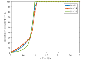
According to Lemma 2 in [23], suppose 𝐡~=l=1Lαl(𝐚R(ϕl)𝐚TH(θl))~𝐡superscriptsubscript𝑙1𝐿subscript𝛼𝑙tensor-productsubscript𝐚𝑅subscriptitalic-ϕ𝑙superscriptsubscript𝐚𝑇𝐻subscript𝜃𝑙\mathbf{\tilde{h}}=\sum\limits_{l=1}^{L}\alpha_{l}(\mathbf{a}_{R}(\phi_{l})\otimes\mathbf{a}_{T}^{H}(\theta_{l})) is the solution to (33). If N¯=min(Nt,Nr)1025¯𝑁subscript𝑁𝑡subscript𝑁𝑟1025\bar{N}=\min(N_{t},N_{r})\geq 1025 and Δ=infmnsup{|θmθn|,|ϕmϕn|}4.76N¯1Δsubscriptinfimum𝑚𝑛supremumsubscript𝜃𝑚subscript𝜃𝑛subscriptitalic-ϕ𝑚subscriptitalic-ϕ𝑛4.76¯𝑁1\Delta=\inf\limits_{m\neq n}\sup\left\{|\theta_{m}-\theta_{n}|,|\phi_{m}-\phi_{n}|\right\}\geq\frac{4.76}{\bar{N}-1}, then 𝚿𝚿\mathbf{\Psi} given by (33) satisfies rank(𝚿)=L𝚿𝐿(\mathbf{\Psi})=L. It is worth noting that the condition N¯1025¯𝑁1025\bar{N}\geq 1025 is a technical requirement that originally comes from Theorem 1.3 of [33]. In Fig. 2, we illustrate via simulations that rank(𝚿)=L𝚿𝐿(\mathbf{\Psi})=L holds even for small N¯¯𝑁\bar{N} as long as (N¯1)Δ¯𝑁1Δ(\bar{N}-1)\Delta is larger than a certain threshold.

Refer to caption
Figure 2: The probability that rank(𝚿)=L𝚿𝐿(\mathbf{\Psi})=L vs. (N¯1)Δ¯𝑁1Δ(\bar{N}-1)\Delta. We set L=4𝐿4L=4 in the simulations.

Hence, given the upper bound on the number of paths, say L¯¯𝐿\bar{L}, we can introduce the constraint of rank(𝚿𝚿\mathbf{\Psi}) L¯absent¯𝐿\leq\bar{L} into (33), whereby reducing the dimension of the positive semidefinite matrix in (33) to (NtNr+1)×L¯(NtNr+1)2much-less-thansubscript𝑁𝑡subscript𝑁𝑟1¯𝐿superscriptsubscript𝑁𝑡subscript𝑁𝑟12(N_{t}N_{r}+1)\times\bar{L}\ll{(N_{t}N_{r}+1)}^{2}.

In particular, we introduce the following non-convex factorization [30]. Let 𝚿=𝚪𝚪H𝚿𝚪superscript𝚪𝐻\mathbf{\Psi}=\mathbf{\Gamma}\mathbf{\Gamma}^{H}, with 𝚪=[𝚪0T𝚪1T]T(NtNr+1)×L¯𝚪superscriptdelimited-[]superscriptsubscript𝚪0𝑇superscriptsubscript𝚪1𝑇𝑇superscriptsubscript𝑁𝑡subscript𝑁𝑟1¯𝐿\mathbf{\Gamma}=[\mathbf{\Gamma}_{0}^{T}~{}~{}\mathbf{\Gamma}_{1}^{T}]^{T}\in\mathbb{C}^{(N_{t}N_{r}+1)\times\bar{L}}, 𝚪0NtNr×L¯subscript𝚪0superscriptsubscript𝑁𝑡subscript𝑁𝑟¯𝐿\mathbf{\Gamma}_{0}\in\mathbb{C}^{N_{t}N_{r}\times\bar{L}} and 𝚪11×L¯subscript𝚪1superscript1¯𝐿\mathbf{\Gamma}_{1}\in\mathbb{C}^{1\times\bar{L}}, then we have 𝒯(𝐕)=𝚿0=𝚪0𝚪0H𝒯𝐕subscript𝚿0subscript𝚪0superscriptsubscript𝚪0𝐻{\mathcal{T}}({\mathbf{V}})=\mathbf{\Psi}_{0}=\mathbf{\Gamma}_{0}\mathbf{\Gamma}_{0}^{H}, 𝐡~=𝚪0𝚪1H~𝐡subscript𝚪0superscriptsubscript𝚪1𝐻\mathbf{\tilde{h}}=\mathbf{\Gamma}_{0}\mathbf{\Gamma}_{1}^{H} and ε=𝚪1𝚪1H𝜀subscript𝚪1superscriptsubscript𝚪1𝐻\varepsilon=\mathbf{\Gamma}_{1}\mathbf{\Gamma}_{1}^{H}. This way the constraints 𝚿0succeeds-or-equals𝚿0{\mathbf{\Psi}}\succeq 0 in (33) and rank(𝚿)L¯𝚿¯𝐿(\mathbf{\Psi})\leq\bar{L} are both satisfied. Moreover since 𝒯(𝐕)=𝚿0𝒯𝐕subscript𝚿0{\mathcal{T}}({\mathbf{V}})=\mathbf{\Psi}_{0}, the constraint 𝒫𝒯(𝚿𝟎)=𝚿0subscript𝒫𝒯subscript𝚿0subscript𝚿0\mathbf{\mathcal{P}}_{\mathbf{\mathcal{T}}}(\mathbf{\Psi_{0}})=\mathbf{\Psi}_{0} need to be imposed, where 𝒫𝒯()subscript𝒫𝒯\mathbf{\mathcal{P}}_{\mathbf{\mathcal{T}}}(\cdot) denotes the projection of the input matrix onto a block Toeplitz matrix defined as the same as (25). Specifically, let 𝒫𝒯(𝚿0)=𝒯(𝔾(𝚿0))subscript𝒫𝒯subscript𝚿0𝒯𝔾subscript𝚿0\mathbf{\mathcal{P}}_{\mathbf{\mathcal{T}}}(\mathbf{\Psi}_{0})=\mathbf{\mathcal{T}}(\mathds{G}(\mathbf{\Psi}_{0})), where G()𝐺G(\cdot) outputs an (2Nt1)×(2Nr1)2subscript𝑁𝑡12subscript𝑁𝑟1(2N_{t}-1)\times(2N_{r}-1) matrix with an NtNr×NtNrsubscript𝑁𝑡subscript𝑁𝑟subscript𝑁𝑡subscript𝑁𝑟N_{t}N_{r}\times N_{t}N_{r} matrix input 𝚿0subscript𝚿0\mathbf{\Psi}_{0}. In particular, if we partition 𝚿0subscript𝚿0\mathbf{\Psi}_{0} into Nr×Nrsubscript𝑁𝑟subscript𝑁𝑟N_{r}\times N_{r} blocks, i.e.,

𝚿0=[𝐃1,1𝐃1,2𝐃1,Nr𝐃2,1𝐃2,2𝐃2,Nr𝐃Nr,1𝐃Nr,2𝐃Nr,Nr]NtNr×NtNr,subscript𝚿0delimited-[]subscript𝐃11subscript𝐃12subscript𝐃1subscript𝑁𝑟missing-subexpressionmissing-subexpressionmissing-subexpressionmissing-subexpressionmissing-subexpressionmissing-subexpressionmissing-subexpressionmissing-subexpressionmissing-subexpressionmissing-subexpressionmissing-subexpressionmissing-subexpressionmissing-subexpressionmissing-subexpressionmissing-subexpressionmissing-subexpressionsubscript𝐃21subscript𝐃22subscript𝐃2subscript𝑁𝑟missing-subexpressionmissing-subexpressionmissing-subexpressionmissing-subexpressionmissing-subexpressionmissing-subexpressionmissing-subexpressionmissing-subexpressionmissing-subexpressionmissing-subexpressionmissing-subexpressionmissing-subexpressionmissing-subexpressionmissing-subexpressionmissing-subexpressionmissing-subexpressionmissing-subexpressionmissing-subexpressionmissing-subexpressionmissing-subexpressionmissing-subexpressionmissing-subexpressionmissing-subexpressionmissing-subexpressionmissing-subexpressionmissing-subexpressionmissing-subexpressionmissing-subexpressionmissing-subexpressionmissing-subexpressionmissing-subexpressionmissing-subexpressionsubscript𝐃subscript𝑁𝑟1subscript𝐃subscript𝑁𝑟2subscript𝐃subscript𝑁𝑟subscript𝑁𝑟missing-subexpressionmissing-subexpressionmissing-subexpressionmissing-subexpressionmissing-subexpressionmissing-subexpressionmissing-subexpressionmissing-subexpressionmissing-subexpressionmissing-subexpressionmissing-subexpressionmissing-subexpressionmissing-subexpressionmissing-subexpressionmissing-subexpressionmissing-subexpressionsuperscriptsubscript𝑁𝑡subscript𝑁𝑟subscript𝑁𝑡subscript𝑁𝑟\displaystyle\mathbf{\Psi}_{0}=\left[{\begin{array}[]{*{20}{c}}{{\mathbf{D}_{1,1}}}&{{\mathbf{D}_{1,2}}}&\cdots&{{\mathbf{D}_{1,{N_{r}}}}}\\ {{\mathbf{D}_{2,1}}}&{{\mathbf{D}_{2,2}}}&\cdots&{{\mathbf{D}_{2,{N_{r}}}}}\\ \vdots&\vdots&\ddots&\vdots\\ {{\mathbf{D}_{{N_{r}},1}}}&{{\mathbf{D}_{{N_{r}},2}}}&\cdots&{{\mathbf{D}_{{N_{r}},{N_{r}}}}}\end{array}}\right]\in\mathbb{C}^{N_{t}N_{r}\times N_{t}N_{r}}, (43)

with the (p,q)𝑝𝑞(p,q)-th element of 𝐃m,nsubscript𝐃𝑚𝑛\mathbf{D}_{m,n} denoted as dp,qm,nsuperscriptsubscript𝑑𝑝𝑞𝑚𝑛d_{p,q}^{m,n}, p,q=1,2,,Nt;m,n=1,2,,Nrformulae-sequence𝑝𝑞12subscript𝑁𝑡𝑚𝑛12subscript𝑁𝑟p,q=1,2,...,N_{t};m,n=1,2,...,N_{r}, then the (i,j)𝑖𝑗(i,j)-th element of 𝔾(𝚿0)𝔾subscript𝚿0\mathds{G}(\mathbf{\Psi}_{0}) is pq=imn=jdp,qm,nκi,jsuperscriptsubscript𝑝𝑞𝑖𝑚𝑛𝑗superscriptsubscript𝑑𝑝𝑞𝑚𝑛subscript𝜅𝑖𝑗\frac{\sum\limits_{p-q=i}^{m-n=j}d_{p,q}^{m,n}}{\kappa_{i,j}}, κi,j=(Nt|i|)(Nr|j|)subscript𝜅𝑖𝑗subscript𝑁𝑡𝑖subscript𝑁𝑟𝑗\kappa_{i,j}=(N_{t}-|i|)(N_{r}-|j|), i=Nt+1,Nt+2,,Nt1,j=Nr+1,Nr+2,,Nr1formulae-sequence𝑖subscript𝑁𝑡1subscript𝑁𝑡2subscript𝑁𝑡1𝑗subscript𝑁𝑟1subscript𝑁𝑟2subscript𝑁𝑟1i=-N_{t}+1,-N_{t}+2,...,N_{t}-1,j=-N_{r}+1,-N_{r}+2,...,N_{r}-1. If we partition 𝒯(𝔾(𝚿0))𝒯𝔾subscript𝚿0\mathbf{\mathcal{T}}(\mathds{G}(\mathbf{\Psi}_{0})) into Nr×Nrsubscript𝑁𝑟subscript𝑁𝑟N_{r}\times N_{r} blocks, e.g., 𝐃~m,nNt×Ntsubscript~𝐃𝑚𝑛superscriptsubscript𝑁𝑡subscript𝑁𝑡\mathbf{\tilde{D}}_{m,n}\in\mathbb{C}^{N_{t}\times N_{t}} with the (p,q)𝑝𝑞(p,q)-th element of 𝐃~m,nsubscript~𝐃𝑚𝑛\mathbf{\tilde{D}}_{m,n} denoted as d~p,qm,nsuperscriptsubscript~𝑑𝑝𝑞𝑚𝑛\tilde{d}_{p,q}^{m,n}, then d~p,qm,n=pq=imn=jdp,qm,nκi,jsuperscriptsubscript~𝑑𝑝𝑞𝑚𝑛superscriptsubscript𝑝𝑞𝑖𝑚𝑛𝑗superscriptsubscript𝑑𝑝𝑞𝑚𝑛subscript𝜅𝑖𝑗\tilde{d}_{p,q}^{m,n}=\frac{\sum\limits_{p-q=i}^{m-n=j}d_{p,q}^{m,n}}{\kappa_{i,j}}. Therefore, the problem defined in (33) can be transformed into

argmin𝚪NtNr×L¯𝐞KMs×1μ2NtNrTr(𝚿0)+12𝐲~((𝐒ˇT+[vec1(𝐞)]T)𝐅T𝐖H)𝐡~22+με2+λ𝐞1subscriptFRACOP𝚪superscriptsubscript𝑁𝑡subscript𝑁𝑟¯𝐿𝐞superscript𝐾subscript𝑀𝑠1𝜇2subscript𝑁𝑡subscript𝑁𝑟Trsubscript𝚿012superscriptsubscriptnorm~𝐲tensor-productsuperscriptˇ𝐒𝑇superscriptdelimited-[]superscriptvec1𝐞𝑇superscript𝐅𝑇superscript𝐖𝐻~𝐡22𝜇𝜀2𝜆subscriptnorm𝐞1\displaystyle\arg\min\limits_{\mathbf{\Gamma}\in\mathbb{C}^{N_{t}N_{r}\times\bar{L}}\hfill\atop\mathbf{e}\in\mathbb{C}^{KM_{s}\times 1}}\frac{\mu}{2N_{t}N_{r}}\mathrm{Tr}(\mathbf{\Psi}_{0})+\frac{1}{2}\left\|{{{\tilde{\mathbf{y}}}}-((\check{\mathbf{S}}^{T}+[\mathrm{vec}^{-1}(\mathbf{e})]^{T})\mathbf{F}^{T}\otimes\mathbf{W}^{H}){{\tilde{\mathbf{h}}}}}\right\|_{2}^{2}+\frac{\mu\varepsilon}{2}+\lambda\|\mathbf{e}\|_{1} (44)
s.t.𝒯(𝔾(𝚿0))=𝚿0.\displaystyle\rm{s.t.}~{}~{}~{}~{}\mathbf{\mathcal{T}}(\mathds{G}(\mathbf{\Psi}_{0}))=\mathbf{\Psi}_{0}.

IV-B Conjugate Gradient Descent Algorithm

To solve (44), we first transform it into a smooth unconstrained optimization problem and then apply the CGD method to solve it. In particular we replace the constraint 𝒫𝒯(𝚿0)=𝚿0subscript𝒫𝒯subscript𝚿0subscript𝚿0\mathbf{\mathcal{P}}_{\mathbf{\mathcal{T}}}(\mathbf{\Psi}_{0})=\mathbf{\Psi}_{0} with the penalty term ϱ2𝒫𝒯(𝚿0)𝚿0F2italic-ϱ2superscriptsubscriptnormsubscript𝒫𝒯subscript𝚿0subscript𝚿0𝐹2\frac{\varrho}{2}\|\mathbf{\mathcal{P}}_{\mathbf{\mathcal{T}}}(\mathbf{\Psi}_{0})-\mathbf{\Psi}_{0}\|_{F}^{2} in the objective function. Moreover, since 1\|\cdot\|_{1} in the objective function is non-smooth, we approximate it with

𝐞1ψτ(𝐞)=τm=1KMslogcosh(|em|/τ),subscriptnorm𝐞1subscript𝜓𝜏𝐞𝜏superscriptsubscript𝑚1𝐾subscript𝑀𝑠subscript𝑒𝑚𝜏\|\mathbf{e}\|_{1}\approx\psi_{\tau}(\mathbf{e})=\tau\sum\limits_{m=1}^{KM_{s}}\log\cosh(|e_{m}|/\tau), (45)

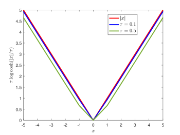
where 𝐞=[e1,e2,,eKMs]T𝐞superscriptsubscript𝑒1subscript𝑒2subscript𝑒𝐾subscript𝑀𝑠𝑇\mathbf{e}=[e_{1},e_{2},...,e_{KM_{s}}]^{T} and the parameter τ𝜏\tau controls the smoothing level as illustrated in Fig. 3.
Refer to caption
Figure 3: The smooth 1subscript1\ell_{1}-norm surrogate defined in (45). The surrogate approximates the 1subscript1\ell_{1}-norm more closely when τ𝜏\tau gets smaller.

Hence, (44) is replaced by the following unconstrained optimization problem

min𝚪(NtNr+1)×L¯𝐞KMs×1ζ(𝚪𝚪H,𝐞),subscriptFRACOP𝚪superscriptsubscript𝑁𝑡subscript𝑁𝑟1¯𝐿𝐞superscript𝐾subscript𝑀𝑠1𝜁𝚪superscript𝚪𝐻𝐞\min\limits_{\mathbf{\Gamma}\in\mathbb{C}^{(N_{t}N_{r}+1)\times\bar{L}}\hfill\atop\mathbf{e}\in\mathbb{C}^{KM_{s}\times 1}}~{}~{}\zeta(\mathbf{\Gamma}\mathbf{\Gamma}^{H},\mathbf{e}), (46)

where

ζ(𝚪𝚪H,𝐞)𝜁𝚪superscript𝚪𝐻𝐞\displaystyle\zeta(\mathbf{\Gamma}\mathbf{\Gamma}^{H},\mathbf{e}) =μ2NtNrTr(𝚿0)+με2+12𝐲~((𝐒ˇT+[vec1(𝐞)]T)𝐅T𝐖H𝚯)𝐡~22absent𝜇2subscript𝑁𝑡subscript𝑁𝑟Trsubscript𝚿0𝜇𝜀212superscriptsubscriptnorm~𝐲subscripttensor-productsuperscriptˇ𝐒𝑇superscriptdelimited-[]superscriptvec1𝐞𝑇superscript𝐅𝑇superscript𝐖𝐻𝚯~𝐡22\displaystyle=\frac{\mu}{2N_{t}N_{r}}\mathrm{Tr}(\mathbf{\Psi}_{0})+\frac{\mu\varepsilon}{2}+\frac{1}{2}\left\|{{{\tilde{\mathbf{y}}}}-(\underbrace{(\check{\mathbf{S}}^{T}+[\mathrm{vec}^{-1}(\mathbf{e})]^{T})\mathbf{F}^{T}\otimes\mathbf{W}^{H}}_{\mathbf{\Theta}}){\tilde{\mathbf{h}}}}\right\|_{2}^{2} (47)
+ϱ2𝒯(𝔾(𝚿0))𝚿0F2+λψτ(𝐞).italic-ϱ2superscriptsubscriptnorm𝒯𝔾subscript𝚿0subscript𝚿0𝐹2𝜆subscript𝜓𝜏𝐞\displaystyle+\frac{\varrho}{2}\|\mathbf{\mathcal{T}}(\mathds{G}(\mathbf{\Psi}_{0}))-\mathbf{\Psi}_{0}\|_{F}^{2}+\lambda\psi_{\tau}(\mathbf{e}).

The CGD algorithm [31] for solving (47) performs the following iterations

𝚪superscript𝚪\displaystyle\mathbf{\Gamma}^{\ell} =\displaystyle= 𝚪1+ς𝐁,superscript𝚪1superscript𝜍superscript𝐁\displaystyle\mathbf{\Gamma}^{\ell-1}+\varsigma^{\ell}\mathbf{B}^{\ell}, (48)
𝐞superscript𝐞\displaystyle\mathbf{e}^{\ell} =\displaystyle= 𝐞1+ς𝐛,superscript𝐞1superscript𝜍superscript𝐛\displaystyle\mathbf{e}^{\ell-1}+\varsigma^{\ell}\mathbf{b}^{\ell}, (49)

where ςsuperscript𝜍\varsigma^{\ell} is the step size, 𝐛superscript𝐛\mathbf{b}^{\ell} and 𝐁superscript𝐁\mathbf{B}^{\ell} are the search directions at step \ell, evaluated as the weighted sum of the gradient at present iteration and the search direction used at the previous iteration. Specifically, let 𝚪ζsuperscriptsubscript𝚪𝜁\nabla_{\mathbf{\Gamma}}^{\ell}\zeta and 𝐞ζsuperscriptsubscript𝐞𝜁\nabla_{\mathbf{e}}^{\ell}\zeta be the gradients of ζ(𝚪𝚪H,𝐞)𝜁𝚪superscript𝚪𝐻𝐞\zeta(\mathbf{\Gamma}\mathbf{\Gamma}^{H},\mathbf{e}) at the \ell-th iteration, then we have

𝐁superscript𝐁\displaystyle\mathbf{B}^{\ell} =\displaystyle= 𝚪ζ+ω𝐁1,superscriptsubscript𝚪𝜁superscript𝜔superscript𝐁1\displaystyle-\nabla_{\mathbf{\Gamma}}^{\ell}\zeta+\omega^{\ell}\mathbf{B}^{\ell-1}, (50)
𝐛superscript𝐛\displaystyle\mathbf{b}^{\ell} =\displaystyle= 𝐞ζ+ω𝐛1,superscriptsubscript𝐞𝜁superscript𝜔superscript𝐛1\displaystyle-\nabla_{\mathbf{e}}^{\ell}\zeta+\omega^{\ell}\mathbf{b}^{\ell-1}, (51)

where

ω=𝚪ζ,𝐑+𝐞ζ,𝐫𝐁1,𝐑+𝐛1,𝐫,superscript𝜔superscriptsubscript𝚪𝜁superscript𝐑superscriptsubscript𝐞𝜁superscript𝐫superscript𝐁1superscript𝐑superscript𝐛1superscript𝐫\omega^{\ell}=\frac{\langle\nabla_{\mathbf{\Gamma}}^{\ell}\zeta,\mathbf{R}^{\ell}\rangle+\langle\nabla_{\mathbf{e}}^{\ell}\zeta,\mathbf{r}^{\ell}\rangle}{\langle\mathbf{B}^{\ell-1},\mathbf{R}^{\ell}\rangle+\langle\mathbf{b}^{\ell-1},\mathbf{r}^{\ell}\rangle}, (52)

with 𝐀,𝐂𝐀𝐂\langle\mathbf{A},\mathbf{C}\rangle being defined as 𝐀,𝐂=Tr(𝐂H𝐀)𝐀𝐂Trsuperscript𝐂𝐻𝐀\langle\mathbf{A},\mathbf{C}\rangle=\mathrm{Tr}(\mathbf{C}^{H}\mathbf{A}), and

𝐑superscript𝐑\displaystyle\mathbf{R}^{\ell} =\displaystyle= 𝚪ζ𝚪1ζ,superscriptsubscript𝚪𝜁superscriptsubscript𝚪1𝜁\displaystyle\nabla_{\mathbf{\Gamma}}^{\ell}\zeta-\nabla_{\mathbf{\Gamma}}^{\ell-1}\zeta, (53)
𝐫superscript𝐫\displaystyle\mathbf{r}^{\ell} =\displaystyle= 𝐞ζ𝐞1ζ.superscriptsubscript𝐞𝜁superscriptsubscript𝐞1𝜁\displaystyle\nabla_{\mathbf{e}}^{\ell}\zeta-\nabla_{\mathbf{e}}^{\ell-1}\zeta. (54)

The expressions of the gradients 𝚪ζsuperscriptsubscript𝚪𝜁\nabla_{\mathbf{\Gamma}}^{\ell}\zeta and 𝐞ζsuperscriptsubscript𝐞𝜁\nabla_{\mathbf{e}}^{\ell}\zeta are derived in Appendix.

Note that the above CGD algorithm can also be used to solve the data-aided channel estimation problem for the GSM system, by replacing 𝚯𝚯\mathbf{\Theta} in (47) with (𝐗ˇT+𝐄T)𝐖Htensor-productsuperscriptˇ𝐗𝑇superscript𝐄𝑇superscript𝐖𝐻(\check{\mathbf{X}}^{T}+\mathbf{E}^{T})\otimes\mathbf{W}^{H}. Moreover, the CGD algorithm can be used to solve the pilot-assisted channel estimation problem in (27) as well, i.e., using 𝐞=𝟎KMs×1𝐞subscript0𝐾subscript𝑀𝑠1\mathbf{e}=\mathbf{0}_{KM_{s}\times 1}, 𝚯=(𝐒T𝐅T)𝐖H𝚯tensor-productsuperscript𝐒𝑇superscript𝐅𝑇superscript𝐖𝐻\mathbf{\Theta}=(\mathbf{S}^{T}\mathbf{F}^{T})\otimes\mathbf{W}^{H} for the HB system and 𝚯=𝐗T𝐖H𝚯tensor-productsuperscript𝐗𝑇superscript𝐖𝐻\mathbf{\Theta}=\mathbf{X}^{T}\otimes\mathbf{W}^{H} for the GSM system, respectively.

For clarity, we summarize the proposed non-convex solver for the Atom-DA-HB estimator in Algorithm 1, Algorithm 2 and Algorithm 3, and the algorithms of the Atom-DA-GSM estimator and the Atom-pilot estimator are similar. To guarantee that the objective function does not increase with \ell, the Armijo line search [32] is employed (line 10 of Algorithm 2 and line 11 of Algorithm 3), so that the algorithm converges to a stationary point of the surrogate problem, namely, the point where the smoothed objective function (47) has vanishing gradient.

Algorithm 1 Atom-DA-HB estimator
0:  T𝑇T, K𝐾K, Mssubscript𝑀𝑠M_{s}, 𝐒0subscript𝐒0\mathbf{S}_{0} and {𝐘t}t=0Tsuperscriptsubscriptsubscript𝐘𝑡𝑡0𝑇\{\mathbf{Y}_{t}\}_{t=0}^{T}
0:  𝐇^=[𝐇^1,𝐇^2,,𝐇^T]^𝐇subscript^𝐇1subscript^𝐇2subscript^𝐇𝑇\hat{\mathbf{H}}=[\hat{\mathbf{H}}_{1},\hat{\mathbf{H}}_{2},...,\hat{\mathbf{H}}_{T}]
1:  t=0𝑡0t=0.
2:  𝐡^0=CGPilot(K,Ms,𝐒0,𝐅0,𝐖0,𝐘0)subscript^𝐡0CGPilot𝐾subscript𝑀𝑠subscript𝐒0subscript𝐅0subscript𝐖0subscript𝐘0\hat{\mathbf{h}}_{0}=\mathrm{CGPilot}(K,M_{s},\mathbf{S}_{0},\mathbf{F}_{0},\mathbf{W}_{0},\mathbf{Y}_{0}), 𝐇^0=vec1(𝐡^0)subscript^𝐇0superscriptvec1subscript^𝐡0\hat{\mathbf{H}}_{0}=\mathrm{vec}^{-1}(\hat{\mathbf{h}}_{0}).
3:  Set 𝐅1subscript𝐅1\mathbf{F}_{1} and 𝐖1subscript𝐖1\mathbf{W}_{1} using 𝐇^0subscript^𝐇0\mathbf{\hat{H}}_{0} according to, e.g., [18].
4:  for t=1𝑡1t=1 to T𝑇T do
5:     Obtain 𝐒ˇtsubscriptˇ𝐒𝑡\check{\mathbf{S}}_{t} using (30).
6:     (𝐡^t,𝐞^t)=CGData(K,Ms,𝐒ˇt,𝐅t,𝐖t,𝐘t)subscript^𝐡𝑡subscript^𝐞𝑡CGData𝐾subscript𝑀𝑠subscriptˇ𝐒𝑡subscript𝐅𝑡subscript𝐖𝑡subscript𝐘𝑡(\hat{\mathbf{h}}_{t},\hat{\mathbf{e}}_{t})=\mathrm{CGData}(K,M_{s},\check{\mathbf{S}}_{t},\mathbf{F}_{t},\mathbf{W}_{t},\mathbf{Y}_{t}).
7:     𝐇^t=vec1(𝐡^t)subscript^𝐇𝑡superscriptvec1subscript^𝐡𝑡\hat{\mathbf{H}}_{t}=\mathrm{vec}^{-1}(\hat{\mathbf{h}}_{t}), 𝐄^t=vec1(𝐞^t)subscript^𝐄𝑡superscriptvec1subscript^𝐞𝑡\hat{\mathbf{E}}_{t}=\mathrm{vec}^{-1}(\hat{\mathbf{e}}_{t}), and update 𝐒^tsubscript^𝐒𝑡\hat{\mathbf{S}}_{t} using (34);
8:     Update 𝐅t+1subscript𝐅𝑡1\mathbf{F}_{t+1} and 𝐖t+1subscript𝐖𝑡1\mathbf{W}_{t+1} using 𝐇^tsubscript^𝐇𝑡\mathbf{\hat{H}}_{t} according to, e.g., [18].
9:  end for
Algorithm 2   𝐡^^𝐡\hat{\mathbf{h}} = CGPilot(K,Ms,𝐒0,𝐅0,𝐖0,𝐘0)𝐾subscript𝑀𝑠subscript𝐒0subscript𝐅0subscript𝐖0subscript𝐘0(K,M_{s},\mathbf{S}_{0},\mathbf{F}_{0},\mathbf{W}_{0},\mathbf{Y}_{0})
0:  ϵitalic-ϵ\epsilon, K𝐾K, Mssubscript𝑀𝑠M_{s}, ϱitalic-ϱ\varrho, μ𝜇\mu, 𝐘0subscript𝐘0\mathbf{Y}_{0} and 𝐒0subscript𝐒0\mathbf{S}_{0}
0:  𝐡^^𝐡\hat{\mathbf{h}}
1:  =00\ell=0.
2:  Do
3:  +11\ell\leftarrow\ell+1.
4:  Calculate 𝚪ζsuperscriptsubscript𝚪𝜁\nabla_{\mathbf{\Gamma}}^{\ell}\zeta using (59), (62), (63) and (71).
5:  if =11\ell=1 then
6:     𝐁=𝚪ζsuperscript𝐁superscriptsubscript𝚪𝜁\mathbf{B}^{\ell}=-\nabla_{\mathbf{\Gamma}}^{\ell}\zeta,
7:  else
8:     Calculate 𝐁superscript𝐁\mathbf{B}^{\ell} using (50), (52)-(48).
9:  end if
10:  Update 𝚪superscript𝚪\mathbf{\Gamma}^{\ell} using (48) with ςsuperscript𝜍\varsigma^{\ell} obtained via Armijo line search.
11:  While 𝚪ζF>ϵsubscriptnormsuperscriptsubscript𝚪𝜁𝐹italic-ϵ\|\nabla_{\mathbf{\Gamma}}^{\ell}\zeta\|_{F}>\epsilon.
12:  𝐡^=𝚪0(𝚪1)H^𝐡superscriptsubscript𝚪0superscriptsuperscriptsubscript𝚪1𝐻\hat{\mathbf{h}}=\mathbf{\Gamma}_{0}^{\ell}(\mathbf{\Gamma}_{1}^{\ell})^{H} with 𝚪=[(𝚪0)T(𝚪1)T]Tsuperscript𝚪superscriptdelimited-[]superscriptsuperscriptsubscript𝚪0𝑇superscriptsuperscriptsubscript𝚪1𝑇𝑇\mathbf{\Gamma}^{\ell}=[(\mathbf{\Gamma}_{0}^{\ell})^{T}~{}(\mathbf{\Gamma}_{1}^{\ell})^{T}]^{T}.
Algorithm 3   (𝐡^,𝐞^)^𝐡^𝐞(\hat{\mathbf{h}},\hat{\mathbf{e}}) = CGData(K,Ms,𝐒ˇt,𝐅t,𝐖t,𝐘t)𝐾subscript𝑀𝑠subscriptˇ𝐒𝑡subscript𝐅𝑡subscript𝐖𝑡subscript𝐘𝑡(K,M_{s},\check{\mathbf{S}}_{t},\mathbf{F}_{t},\mathbf{W}_{t},\mathbf{Y}_{t})
0:  ϵitalic-ϵ\epsilon, K𝐾K, Mssubscript𝑀𝑠M_{s}, ϱitalic-ϱ\varrho, μ𝜇\mu, τ𝜏\tau, λ𝜆\lambda, 𝐘tsubscript𝐘𝑡\mathbf{Y}_{t} and 𝐒ˇtsubscriptˇ𝐒𝑡\check{\mathbf{S}}_{t}
0:  𝐡^^𝐡\hat{\mathbf{h}}, 𝐞^^𝐞\hat{\mathbf{e}}
1:  =00\ell=0.
2:  Do
3:  =+11\ell=\ell+1.
4:  Calculate 𝐞ζsuperscriptsubscript𝐞𝜁\nabla_{\mathbf{e}}^{\ell}\zeta using (57) and (58).
5:  Calculate 𝚪ζsuperscriptsubscript𝚪𝜁\nabla_{\mathbf{\Gamma}}^{\ell}\zeta using (59), (62), (63) and (71).
6:  if =11\ell=1 then
7:     𝐁=𝚪ζsuperscript𝐁superscriptsubscript𝚪𝜁\mathbf{B}^{\ell}=-\nabla_{\mathbf{\Gamma}}^{\ell}\zeta, 𝐛=𝐞ζsuperscript𝐛superscriptsubscript𝐞𝜁\mathbf{b}^{\ell}=-\nabla_{\mathbf{e}}^{\ell}\zeta,
8:  else
9:     Calculate 𝐁superscript𝐁\mathbf{B}^{\ell} and 𝐛superscript𝐛\mathbf{b}^{\ell} using (50)-(48).
10:  end if
11:  Update 𝚪superscript𝚪\mathbf{\Gamma}^{\ell} and 𝐞superscript𝐞\mathbf{e}^{\ell} using (48) and (43) with ςsuperscript𝜍\varsigma^{\ell} obtained via Armijo line search.
12:  While 𝚪ζF>ϵsubscriptnormsuperscriptsubscript𝚪𝜁𝐹italic-ϵ\|\nabla_{\mathbf{\Gamma}}^{\ell}\zeta\|_{F}>\epsilon.
13:  𝐡^=𝚪0(𝚪1)H^𝐡superscriptsubscript𝚪0superscriptsuperscriptsubscript𝚪1𝐻\hat{\mathbf{h}}=\mathbf{\Gamma}_{0}^{\ell}(\mathbf{\Gamma}_{1}^{\ell})^{H} with 𝚪=[(𝚪0)T(𝚪1)T]Tsuperscript𝚪superscriptdelimited-[]superscriptsuperscriptsubscript𝚪0𝑇superscriptsuperscriptsubscript𝚪1𝑇𝑇\mathbf{\Gamma}^{\ell}=[(\mathbf{\Gamma}_{0}^{\ell})^{T}~{}(\mathbf{\Gamma}_{1}^{\ell})^{T}]^{T}, 𝐞^=𝐞^𝐞superscript𝐞\hat{\mathbf{e}}=\mathbf{e}^{\ell}.

V Simulation Results

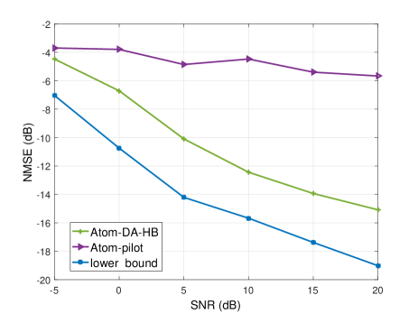
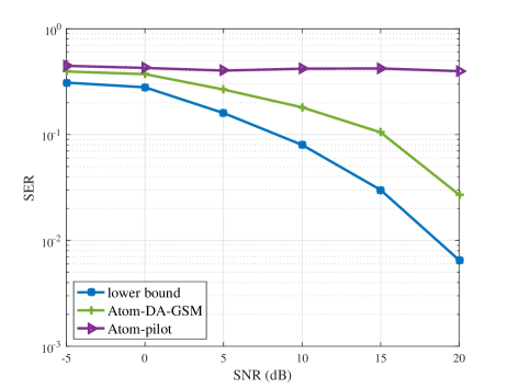
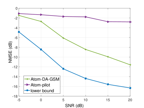
In this section, we use simulations to illustrate the performance of the proposed algorithms in both the HB and GSM systems. The uniform linear arrays at the transmitter and receiver are equipped with Nt=Nr=16subscript𝑁𝑡subscript𝑁𝑟16N_{t}=N_{r}=16 antennas and nt=nr=2subscript𝑛𝑡subscript𝑛𝑟2n_{t}=n_{r}=2 RF chains, respectively. The channel matrix is generated according to (1) where {θl,ϕl}l=1Lsuperscriptsubscriptsubscript𝜃𝑙subscriptitalic-ϕ𝑙𝑙1𝐿\{\theta_{l},\phi_{l}\}_{l=1}^{L} are uniformly generated within the interval of [0,1)01[0,1) and the path amplitudes {αl}l=1Lsuperscriptsubscriptsubscript𝛼𝑙𝑙1𝐿\{\alpha_{l}\}_{l=1}^{L} are randomly generated according to distribution 𝒞𝒩(0,σl2)𝒞𝒩0superscriptsubscript𝜎𝑙2\mathcal{CN}(0,\sigma_{l}^{2}) with equal variances, i.e., σl2=1,l=1,2,,Lformulae-sequencesuperscriptsubscript𝜎𝑙21𝑙12𝐿\sigma_{l}^{2}=1,l=1,2,...,L. Following the setting of [16], the average number of resolvable paths ranges from 1 to 8. The number of time blocks is T=100𝑇100T=100 and QPSK modulation is employed. The signal-to-noise ratio (SNR) is defined as PNtσ2𝑃subscript𝑁𝑡superscript𝜎2\frac{P}{N_{t}\sigma^{2}} with P𝑃P denoting the average transmission power. We use the normalized mean-square error (NMSE) defined as 10log10(𝔼[𝐇𝐇^F2/𝐇F2])10subscript10𝔼delimited-[]superscriptsubscriptnorm𝐇^𝐇𝐹2superscriptsubscriptnorm𝐇𝐹210\log_{10}(\mathbb{E}[\|\mathbf{H}-\hat{\mathbf{H}}\|_{F}^{2}/\|\mathbf{H}\|_{F}^{2}]) to evaluate the performance of channel estimation, and the symbol error rates (SERs) defined as 𝔼[k=1Kη(𝐬k𝐬^k)/K]𝔼delimited-[]superscriptsubscript𝑘1𝐾𝜂subscript𝐬𝑘subscript^𝐬𝑘𝐾\mathbb{E}[\sum_{k=1}^{K}\eta(\mathbf{s}_{k}-\hat{\mathbf{s}}_{k})/K] for the HB system and 𝔼[k=1Kη(𝐱k𝐱^k)/K]𝔼delimited-[]superscriptsubscript𝑘1𝐾𝜂subscript𝐱𝑘subscript^𝐱𝑘𝐾\mathbb{E}[\sum_{k=1}^{K}\eta(\mathbf{x}_{k}-\hat{\mathbf{x}}_{k})/K] for the GSM system with η(𝐟,𝐟^)=0𝜂𝐟^𝐟0\eta(\mathbf{f},\hat{\mathbf{f}})=0 if 𝐟=𝐟^𝐟^𝐟\mathbf{f}=\hat{\mathbf{f}}; else η(𝐟,𝐟^)=1𝜂𝐟^𝐟1\eta(\mathbf{f},\hat{\mathbf{f}})=1, to evaluate the performance of symbol demodulation.

V-A Convergence of the Conjugate Gradient Descent Algorithm

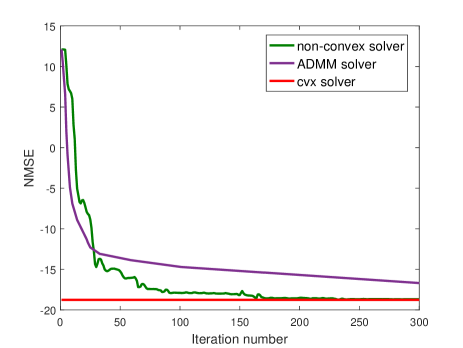
The computational complexity of the proposed CGD algorithm at each iteration is mainly determined by the calculation of 𝚪𝚪H𝚪superscript𝚪𝐻\mathbf{\Gamma}\mathbf{\Gamma}^{H}, whose complexity is 𝒪(Nt2Nr2L¯)𝒪superscriptsubscript𝑁𝑡2superscriptsubscript𝑁𝑟2¯𝐿\mathcal{O}(N_{t}^{2}N_{r}^{2}\bar{L}). As L¯NtNrmuch-less-than¯𝐿subscript𝑁𝑡subscript𝑁𝑟\bar{L}\ll N_{t}N_{r}, the complexity per iteration is much smaller than that of a classical eigenvalue decomposition, whereby, for large-dimensional problems, the proposed non-convex approach can be faster than those based on the first-order methods such as ADMM. We illustrate this fact through simulation examples, whose results are reported in Fig. 4. The parameters are SNR = 101010dB, L=5𝐿5L=5 and K=8𝐾8K=8. The non-convex solver is implemented by solving (46) with the CGD algorithm. We compare the NMSE of the proposed algorithm with that given by solving (28) with the CVX [34] and ADMM [24] solvers. As can be seen from Fig. 4, the results of the proposed algorithm is close to the solution given by the CVX after 300 iterations. Because the proposed algorithm runs much faster than the ADMM, it appears much more suitable for real-time implementation.
Refer to caption
Figure 4: Convergence behavior of the proposed non-convex solver. The non-convex solver takes 34 seconds with 300 iterations, the ADMM solver takes 142 seconds with 300 iterations, and the CVX solver of the Atom-pilot estimator takes 359 seconds in the HB system.

V-B Pilot-assisted Channel Estimation

To compared with the proposed Atom-pilot estimators, we consider two grid-based compressed sensing methods for performance comparison with the Atom-pilot estimators, i.e., the OMP and CS-L1 algorithms discussed in Section III, where the continuous parameter space [0,1)×[0,1)0101[0,1)\times[0,1) is discretized into a finite set of grids with Ngsubscript𝑁𝑔N_{g} grid points. For the Atom-pilot estimator, we use the CVX solver to solve (28), and the proposed non-convex solver to solve (46) with 𝐞=𝟎KMs×1𝐞subscript0𝐾subscript𝑀𝑠1\mathbf{e}=\mathbf{0}_{KM_{s}\times 1}, randomly initialized 𝚪0superscript𝚪0\mathbf{\Gamma}^{0}, L¯=9¯𝐿9\bar{L}=9 and ϱ=5italic-ϱ5\varrho=5. The algorithm stops as the gradient norm is smaller than ϵ=0.01italic-ϵ0.01\epsilon=0.01. The weighting parameter is set as μ=σNtNrlog(NtNr)𝜇𝜎subscript𝑁𝑡subscript𝑁𝑟subscript𝑁𝑡subscript𝑁𝑟\mu=\sigma\sqrt{N_{t}N_{r}\log(N_{t}N_{r})} [25].

During the pilot training stage, for the HB system, the analog filters 𝐅Asubscript𝐅𝐴\mathbf{F}_{A} and 𝐖Asubscript𝐖𝐴\mathbf{W}_{A} are designed according to (8) and (9) respectively; for the GSM system, 𝐖Asubscript𝐖𝐴\mathbf{W}_{A} is designed according to (9).

Refer to caption

(a)

Refer to caption

(b)

Refer to caption

(c)

Refer to caption

(d)

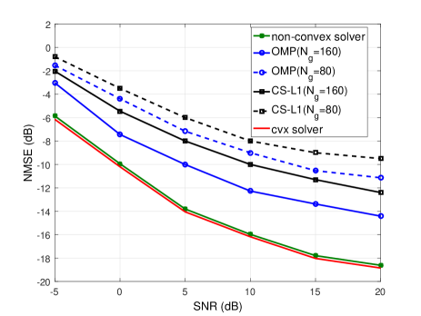
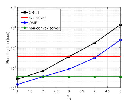
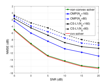
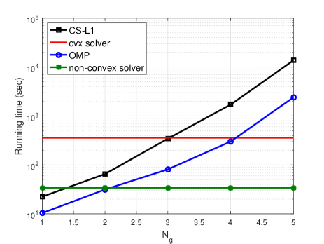
Figure 5: (a) NMSE performance of the Atom-pilot estimator in the HB system, L𝐿L=3, K𝐾K=8; (b) Running times for different estimators in the HB system, SNR=10dB; (c) NMSE performance of the Atom-pilot estimator in the GSM system, L𝐿L=3, K𝐾K=8; (d) Running times for different estimator in the GSM system, SNR=10dB.

As shown in Fig. 5(a), under the same Ngsubscript𝑁𝑔N_{g}, the accuracy of the OMP is always better than that of the CS-L1 algorithm, partly because the number of paths is very small, i.e., L=3𝐿3L=3, for which 0subscript0\ell_{0}-minimization usually results in better accuracy [17]. The OMP estimator is outperformed by the proposed Atom-pilot estimator, especially in the high SNR region. This is due to the fact that, both the CS-L1 and OMP estimators tend to mis-estimate the channel parameters due to basis mismatch. When the grids become denser, the NMSE of the OMP and CS-L1 estimators become smaller. However, the computational complexity becomes higher as shown in Fig. 5(b). Fig. 5(c) and Fig. 5(d) show the performance comparisons in the GSM system. The results are similar to those of the HB system.

V-C Data-aided Channel Estimation

Now we consider the performance of the proposed data-aided estimators with slowly time-varying channels. The channel matrices 𝐇t,t=0,1,,Tformulae-sequencesubscript𝐇𝑡𝑡01𝑇\mathbf{H}_{t},t=0,1,...,T are generated according to (1) at the t𝑡t-th time block. More specifically, for t=0𝑡0t=0, αl0superscriptsubscript𝛼𝑙0\alpha_{l}^{0} are generated following complex Gaussian distribution, i.e., αl0𝒞𝒩(0,σl2)similar-tosuperscriptsubscript𝛼𝑙0𝒞𝒩0superscriptsubscript𝜎𝑙2\alpha_{l}^{0}\sim\mathcal{CN}(0,\sigma_{l}^{2}), ϕl0superscriptsubscriptitalic-ϕ𝑙0\phi_{l}^{0} and θl0superscriptsubscript𝜃𝑙0\theta_{l}^{0} are generated following uniform distribution, i.e., ϕl0,θl0U(1,1)similar-tosuperscriptsubscriptitalic-ϕ𝑙0superscriptsubscript𝜃𝑙0U11\phi_{l}^{0},\theta_{l}^{0}\sim\mathrm{U}(-1,1) with U(a,b)U𝑎𝑏\mathrm{U}(a,b) denoting the uniform distribution in the interval (a,b)𝑎𝑏(a,b). To model the time correlation of the channel, at subsequent time blocks (t=1,2,,T)𝑡12𝑇(t=1,2,...,T), the variation of αltsuperscriptsubscript𝛼𝑙𝑡\alpha_{l}^{t}, ϕltsuperscriptsubscriptitalic-ϕ𝑙𝑡\phi_{l}^{t} and θltsuperscriptsubscript𝜃𝑙𝑡\theta_{l}^{t} relative to αlt1superscriptsubscript𝛼𝑙𝑡1\alpha_{l}^{t-1}, ϕlt1superscriptsubscriptitalic-ϕ𝑙𝑡1\phi_{l}^{t-1} and θlt1superscriptsubscript𝜃𝑙𝑡1\theta_{l}^{t-1}, i.e., Δαlt=αltαlt1Δsuperscriptsubscript𝛼𝑙𝑡superscriptsubscript𝛼𝑙𝑡superscriptsubscript𝛼𝑙𝑡1\Delta\alpha_{l}^{t}=\alpha_{l}^{t}-\alpha_{l}^{t-1}, Δϕlt=ϕltϕlt1Δsuperscriptsubscriptitalic-ϕ𝑙𝑡superscriptsubscriptitalic-ϕ𝑙𝑡superscriptsubscriptitalic-ϕ𝑙𝑡1\Delta\phi_{l}^{t}=\phi_{l}^{t}-\phi_{l}^{t-1} and Δθlt=θltθlt1Δsuperscriptsubscript𝜃𝑙𝑡superscriptsubscript𝜃𝑙𝑡superscriptsubscript𝜃𝑙𝑡1\Delta\theta_{l}^{t}=\theta_{l}^{t}-\theta_{l}^{t-1}, follow distributions 𝒞𝒩(0,0.01σl2)𝒞𝒩00.01superscriptsubscript𝜎𝑙2\mathcal{CN}(0,0.01\sigma_{l}^{2}), U(0.1+ϕlt1,0.1+ϕlt1)U0.1superscriptsubscriptitalic-ϕ𝑙𝑡10.1superscriptsubscriptitalic-ϕ𝑙𝑡1\mathrm{U}(-0.1+\phi_{l}^{t-1},0.1+\phi_{l}^{t-1}) and U(0.1+θlt1,0.1+θlt1)U0.1superscriptsubscript𝜃𝑙𝑡10.1superscriptsubscript𝜃𝑙𝑡1\mathrm{U}(-0.1+\theta_{l}^{t-1},0.1+\theta_{l}^{t-1}), respectively. The weighting parameters for regularizing the sparse demodulation error are set as λ=μ/NtNr𝜆𝜇subscript𝑁𝑡subscript𝑁𝑟\lambda=\mu/\sqrt{N_{t}N_{r}} and τ=0.01𝜏0.01\tau=0.01. In this case for the Atom-pilot estimator, it estimates the channel based on the pilot at t=0𝑡0t=0 to obtain 𝐇^0subscript^𝐇0\hat{\mathbf{H}}_{0} and uses it to demodulate the data for subsequent blocks t=1,2,,T𝑡12𝑇t=1,2,...,T. The Atom-DA-HB and Atom-DA-GSM estimators, however, updates the channel matrix at each time block t𝑡t in a data-aided manner. We also simulate the case when the channel matrix in each block is estimated with pilot symbols which serves as the lower bound of the NMSE in channel estimation.
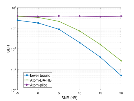
Refer to caption

(a)

Refer to caption

(b)

Refer to caption

(c)

Refer to caption

(d)

Figure 6: Comparison of the estimators performance in the HB system: (a) SER, L𝐿L=8, K𝐾K=8; (b) NMSE, L𝐿L=8, K𝐾K=8; Comparison of the estimators performance in the GSM system: (c) SER, L𝐿L=8, K𝐾K=8; (d) NMSE, L𝐿L=8, K𝐾K=8.

According to Fig. 6(a) and Fig. 6(b), the Atom-pilot estimator cannot work even at high SNR regions. Though there is still a gap of performance between the Atom-DA-HB estimator and the lower bound, the Atom-DA-HB estimator always significantly outperforms the Atom-pilot estimator because it keeps tracking of the time-varying channel dynamics by estimating the channel and demodulation error alternately in each time block. For the Atom-DA-HB estimator, the NMSE curve decreases monotonically with the increasing SNR. This is because that the Atom-DA-HB estimator has better performance on channel estimation with high SNRs; on the other hand, the ML decoder are getting better when the SNR increases, and the demodulation error is getting sparser, in which case the 1subscript1\ell_{1}-norm regularization of the Atom-DA-HB estimator has better performance on demodulation error estimation. We plot both the SER and NMSE performance comparisons of the GSM system in Fig. 6(c) and Fig. 6(d). The results are similar to that of the HB system and the proposed Atom-DA-GSM estimator always performs better than the Atom-pilot estimator.

VI Conclusions

In this paper, we have proposed super-resolution channel estimators for HB-based and GSM-based mmWave systems. For the pilot-assisted scenarios, the proposed channel estimators are based on the atomic norm minimization that exploits the channel sparsity in the continuous angles of departure and arrival. For the data-aided scenario, the proposed channel estimator are based on both atomic norm minimization and 1subscript1\ell_{1}-minimization to exploit the sparsity in both channel and demodulation error. We have developed computationally efficient non-convex methods based on CGD to solve the formulated channel estimators. Simulation results indicate that the proposed algorithms outperform the on-grid CS channel estimators. Moreover, the proposed data-aided estimators can effectively track the time-varying channel dynamics.

-A Gradient Calculations

Firstly, to derive 𝚪ζsubscript𝚪𝜁\nabla_{\mathbf{\Gamma}}\zeta, we rewrite (47) as

ζ(𝚪𝚪H,𝐞)=μ2NtNrTr(𝚿0)+με2+12𝐘𝐖H𝐇𝐅(𝐒ˇ+𝐄)𝚯~F2+ϱ2𝒫𝒯(𝚿0)𝚿0F2+λψτ(𝐞),𝜁𝚪superscript𝚪𝐻𝐞𝜇2subscript𝑁𝑡subscript𝑁𝑟Trsubscript𝚿0𝜇𝜀212superscriptsubscriptnorm𝐘subscriptsuperscript𝐖𝐻𝐇𝐅ˇ𝐒𝐄~𝚯𝐹2italic-ϱ2superscriptsubscriptnormsubscript𝒫𝒯subscript𝚿0subscript𝚿0𝐹2𝜆subscript𝜓𝜏𝐞\zeta(\mathbf{\Gamma}\mathbf{\Gamma}^{H},\mathbf{e})=\frac{\mu}{2N_{t}N_{r}}\mathrm{Tr}(\mathbf{\Psi}_{0})+\frac{\mu\varepsilon}{2}+\frac{1}{2}\left\|{\mathbf{Y}-\underbrace{\mathbf{W}^{H}\mathbf{H}\mathbf{F}(\check{\mathbf{S}}+\mathbf{E})}_{\mathbf{\tilde{\Theta}}}}\right\|_{F}^{2}+\frac{\varrho}{2}\|\mathbf{\mathcal{P}}_{\mathbf{\mathcal{T}}}(\mathbf{\Psi}_{0})-\mathbf{\Psi}_{0}\|_{F}^{2}+\lambda\psi_{\tau}(\mathbf{e}), (55)

where 𝐄=[vec1(𝐞)]𝐄delimited-[]superscriptvec1𝐞\mathbf{E}=[\mathrm{vec}^{-1}(\mathbf{e})]. We have

𝐘𝚯~F2=Tr(𝐘H𝐘)Tr(𝚯~H𝐘)Tr(𝐘H𝚯~)+Tr(𝚯~H𝚯~).superscriptsubscriptnorm𝐘~𝚯𝐹2Trsuperscript𝐘𝐻𝐘Trsuperscript~𝚯𝐻𝐘Trsuperscript𝐘𝐻~𝚯Trsuperscript~𝚯𝐻~𝚯\left\|{\mathbf{Y}-\mathbf{\tilde{\Theta}}}\right\|_{F}^{2}=\mathrm{Tr}({\mathbf{Y}}^{H}\mathbf{Y})-\mathrm{Tr}(\mathbf{\tilde{\Theta}}^{H}\mathbf{Y})-\mathrm{Tr}(\mathbf{Y}^{H}\mathbf{\tilde{\Theta}})+\mathrm{Tr}(\mathbf{\tilde{\Theta}}^{H}\mathbf{\tilde{\Theta}}). (56)

Note that

𝐄i,jTr(𝐘H𝐘)=0,subscriptsubscript𝐄𝑖𝑗Trsuperscript𝐘𝐻𝐘0\displaystyle\nabla_{\mathbf{E}_{i,j}}\mathrm{Tr}({\mathbf{Y}}^{H}\mathbf{Y})=0,
𝐄i,jTr(𝐘H𝚯~)\xlongequal(45)in[35](𝐄j,iTr(𝐘H𝚯~))H=(𝐄j,iTr(𝐘H𝐖H𝐇𝐅𝐄))Hsubscriptsubscript𝐄𝑖𝑗Trsuperscript𝐘𝐻~𝚯\xlongequal45𝑖𝑛delimited-[]35superscriptsubscriptsuperscriptsubscript𝐄𝑗𝑖Trsuperscript𝐘𝐻~𝚯𝐻superscriptsubscriptsuperscriptsubscript𝐄𝑗𝑖Trsuperscript𝐘𝐻superscript𝐖𝐻𝐇𝐅𝐄𝐻\displaystyle\nabla_{\mathbf{E}_{i,j}}\mathrm{Tr}(\mathbf{Y}^{H}\mathbf{\tilde{\Theta}})\xlongequal{(45)~{}in~{}[35]}\left(\nabla_{\mathbf{E}_{j,i}^{*}}\mathrm{Tr}(\mathbf{Y}^{H}\mathbf{\tilde{\Theta}})\right)^{H}=\left(\nabla_{\mathbf{E}_{j,i}^{*}}\mathrm{Tr}(\mathbf{Y}^{H}\mathbf{W}^{H}\mathbf{H}\mathbf{F}\mathbf{E})\right)^{H}
\xlongequal(233),(240),(241)in[35][2𝐘H𝐖H𝐇𝐅]i,jH=[2𝐅H𝐇H𝐖𝐘]i,j,\xlongequal233240241𝑖𝑛delimited-[]35superscriptsubscriptdelimited-[]2superscript𝐘𝐻superscript𝐖𝐻𝐇𝐅𝑖𝑗𝐻subscriptdelimited-[]2superscript𝐅𝐻superscript𝐇𝐻𝐖𝐘𝑖𝑗\displaystyle~{}~{}~{}~{}~{}~{}~{}~{}~{}~{}~{}~{}~{}~{}~{}~{}~{}~{}\xlongequal{(233),(240),(241)~{}in~{}[35]}{[2\mathbf{Y}^{H}\mathbf{W}^{H}\mathbf{H}\mathbf{F}]}_{i,j}^{H}={[2\mathbf{F}^{H}\mathbf{H}^{H}\mathbf{W}\mathbf{Y}]}_{i,j},
𝐄i,jTr(𝚯~H𝐘)=𝐄i,jTr(𝐄H𝐅H𝐇H𝐖𝐘)\xlongequalTr(𝐀𝐁)=Tr(𝐁𝐀)𝐄i,jTr(𝐅H𝐇H𝐖𝐘𝐄H)subscriptsubscript𝐄𝑖𝑗Trsuperscript~𝚯𝐻𝐘subscriptsubscript𝐄𝑖𝑗Trsuperscript𝐄𝐻superscript𝐅𝐻superscript𝐇𝐻𝐖𝐘\xlongequalTr𝐀𝐁Tr𝐁𝐀subscriptsubscript𝐄𝑖𝑗Trsuperscript𝐅𝐻superscript𝐇𝐻superscript𝐖𝐘𝐄𝐻\displaystyle\nabla_{\mathbf{E}_{i,j}}\mathrm{Tr}(\mathbf{\tilde{\Theta}}^{H}\mathbf{Y})=\nabla_{\mathbf{E}_{i,j}}\mathrm{Tr}(\mathbf{E}^{H}\mathbf{F}^{H}\mathbf{H}^{H}\mathbf{W}\mathbf{Y})\xlongequal{\mathrm{Tr}(\mathbf{AB})=\mathrm{Tr}(\mathbf{BA})}\nabla_{\mathbf{E}_{i,j}}\mathrm{Tr}(\mathbf{F}^{H}\mathbf{H}^{H}\mathbf{W}\mathbf{Y}\mathbf{E}^{H})
\xlongequal(233),(240),(241)in[35][2𝐅H𝐇H𝐖𝐘]i,j,\xlongequal233240241𝑖𝑛delimited-[]35subscriptdelimited-[]2superscript𝐅𝐻superscript𝐇𝐻𝐖𝐘𝑖𝑗\displaystyle~{}~{}~{}~{}~{}~{}~{}~{}~{}~{}~{}~{}~{}~{}~{}~{}~{}~{}\xlongequal{(233),(240),(241)~{}in~{}[35]}{[2\mathbf{F}^{H}\mathbf{H}^{H}\mathbf{W}\mathbf{Y}]}_{i,j},
𝐄i,jTr(𝚯~H𝚯~)=𝐄i,jTr(𝐄H𝐉𝐄)+𝐄i,jTr(𝐄H𝐉𝐒ˇ)+𝐄i,jTr(𝐒ˇH𝐉𝐄)subscriptsubscript𝐄𝑖𝑗Trsuperscript~𝚯𝐻~𝚯subscriptsubscript𝐄𝑖𝑗Trsuperscript𝐄𝐻𝐉𝐄subscriptsubscript𝐄𝑖𝑗Trsuperscript𝐄𝐻𝐉ˇ𝐒subscriptsubscript𝐄𝑖𝑗Trsuperscriptˇ𝐒𝐻𝐉𝐄\displaystyle\nabla_{\mathbf{E}_{i,j}}\mathrm{Tr}(\mathbf{\tilde{\Theta}}^{H}\mathbf{\tilde{\Theta}})=\nabla_{\mathbf{E}_{i,j}}\mathrm{Tr}(\mathbf{E}^{H}\mathbf{J}\mathbf{E})+\nabla_{\mathbf{E}_{i,j}}\mathrm{Tr}(\mathbf{E}^{H}\mathbf{J}\mathbf{\check{S}})+\nabla_{\mathbf{E}_{i,j}}\mathrm{Tr}(\mathbf{\check{S}}^{H}\mathbf{J}\mathbf{E})
\xlongequalTr(𝐀𝐁)=Tr(𝐁𝐀)𝐄i,jTr(𝐉𝐄𝐄H)+𝐄i,jTr(𝐉𝐒ˇ𝐄H)+𝐄i,jTr(𝐒ˇH𝐉𝐄)\xlongequalTr𝐀𝐁Tr𝐁𝐀subscriptsubscript𝐄𝑖𝑗Trsuperscript𝐉𝐄𝐄𝐻subscriptsubscript𝐄𝑖𝑗Tr𝐉ˇ𝐒superscript𝐄𝐻subscriptsubscript𝐄𝑖𝑗Trsuperscriptˇ𝐒𝐻𝐉𝐄\displaystyle~{}~{}~{}~{}~{}~{}~{}~{}~{}~{}~{}~{}~{}~{}~{}~{}~{}~{}\xlongequal{\mathrm{Tr}(\mathbf{AB})=\mathrm{Tr}(\mathbf{BA})}\nabla_{\mathbf{E}_{i,j}}\mathrm{Tr}(\mathbf{J}\mathbf{E}\mathbf{E}^{H})+\nabla_{\mathbf{E}_{i,j}}\mathrm{Tr}(\mathbf{J}\mathbf{\check{S}}\mathbf{E}^{H})+\nabla_{\mathbf{E}_{i,j}}\mathrm{Tr}(\mathbf{\check{S}}^{H}\mathbf{J}\mathbf{E})
\xlongequal[chainrule](233),(240),(241)in[35]4𝐉𝐄𝐄i,jTr(𝐉𝐄𝐄H)+2𝐉𝐒ˇ𝐄i,jTr(𝐄H𝐉𝐒ˇ)+2𝐉𝐒ˇ𝐄i,jTr(𝐒ˇH𝐉𝐄)\xlongequaldelimited-[]𝑐𝑎𝑖𝑛𝑟𝑢𝑙𝑒233240241𝑖𝑛delimited-[]35subscript4𝐉𝐄subscriptsubscript𝐄𝑖𝑗Trsuperscript𝐉𝐄𝐄𝐻subscript2𝐉ˇ𝐒subscriptsubscript𝐄𝑖𝑗Trsuperscript𝐄𝐻𝐉ˇ𝐒subscript2𝐉ˇ𝐒subscriptsubscript𝐄𝑖𝑗Trsuperscriptˇ𝐒𝐻𝐉𝐄\displaystyle~{}~{}~{}~{}~{}~{}~{}~{}~{}~{}~{}~{}~{}~{}~{}~{}~{}~{}\xlongequal[chain~{}rule]{(233),(240),(241)~{}in~{}[35]}\underbrace{4\mathbf{J}\mathbf{E}}_{\nabla_{\mathbf{E}_{i,j}}\mathrm{Tr}(\mathbf{J}\mathbf{E}\mathbf{E}^{H})}+\underbrace{2\mathbf{J}\mathbf{\check{S}}}_{\nabla_{\mathbf{E}_{i,j}}\mathrm{Tr}(\mathbf{E}^{H}\mathbf{J}\mathbf{\check{S}})}+\underbrace{2\mathbf{J}\mathbf{\check{S}}}_{\nabla_{\mathbf{E}_{i,j}}\mathrm{Tr}(\mathbf{\check{S}}^{H}\mathbf{J}\mathbf{E})}
=[4𝐉(𝐒ˇ+𝐄)]i,j,𝐉=𝐅H𝐇H𝐖𝐖H𝐇𝐅,formulae-sequenceabsentsubscriptdelimited-[]4𝐉ˇ𝐒𝐄𝑖𝑗𝐉superscript𝐅𝐻superscript𝐇𝐻superscript𝐖𝐖𝐻𝐇𝐅\displaystyle~{}~{}~{}~{}~{}~{}~{}~{}~{}~{}~{}~{}~{}~{}~{}~{}~{}~{}={[4\mathbf{J}(\check{\mathbf{S}}+\mathbf{E})]}_{i,j},\mathbf{J}=\mathbf{F}^{H}\mathbf{H}^{H}\mathbf{W}\mathbf{W}^{H}\mathbf{H}\mathbf{F},

where 𝐄i,jsubscript𝐄𝑖𝑗\mathbf{E}_{i,j} denotes the (i,j)𝑖𝑗(i,j)-th element of 𝐄𝐄\mathbf{E}. Hence

𝐞ζ=vec(2𝐅H𝐇H𝐖(𝐖H𝐇𝐅(𝐒ˇ+vec1(𝐞))𝐘))+λ𝐞ψ,subscript𝐞𝜁vec2superscript𝐅𝐻superscript𝐇𝐻𝐖superscript𝐖𝐻𝐇𝐅ˇ𝐒superscriptvec1𝐞𝐘𝜆subscript𝐞𝜓\nabla_{\mathbf{e}}\zeta=\mathrm{vec}(2\mathbf{F}^{H}\mathbf{H}^{H}\mathbf{W}(\mathbf{W}^{H}\mathbf{H}\mathbf{F}(\check{\mathbf{S}}+\mathrm{vec}^{-1}(\mathbf{e}))-\mathbf{Y}))+\lambda\nabla_{\mathbf{e}}\psi, (57)

where the m𝑚m-th element of 𝐞ψKMs×1subscript𝐞𝜓superscript𝐾subscript𝑀𝑠1\nabla_{\mathbf{e}}\psi\in\mathbb{C}^{KM_{s}\times 1} is

emψ=sinh(|em|/τ)emcosh(|em|/τ)|em|.subscriptsubscript𝑒𝑚𝜓subscript𝑒𝑚𝜏subscript𝑒𝑚subscript𝑒𝑚𝜏subscript𝑒𝑚\nabla_{e_{m}}\psi=\frac{\sinh(|e_{m}|/\tau)e_{m}}{\cosh(|e_{m}|/\tau)|e_{m}|}. (58)

Then we derive 𝚪ζsubscript𝚪𝜁\nabla_{\mathbf{\Gamma}}\zeta. Following the chain rule, we have

𝚪ζ=2[𝚿ζ|𝚿=𝚪𝚪H]𝚪,subscript𝚪𝜁2delimited-[]evaluated-atsubscript𝚿𝜁𝚿𝚪superscript𝚪𝐻𝚪\nabla_{\mathbf{\Gamma}}\zeta=2\left[\nabla_{\mathbf{\Psi}}\zeta|_{\mathbf{\Psi}=\mathbf{\Gamma}\mathbf{\Gamma}^{H}}\right]\mathbf{\Gamma}, (59)

so the problem becomes calculating 𝚿ζsubscript𝚿𝜁\nabla_{\mathbf{\Psi}}\zeta. We have

𝒯(𝔾(𝚿0))𝚿0F2superscriptsubscriptnorm𝒯𝔾subscript𝚿0subscript𝚿0𝐹2\displaystyle\|\mathbf{\mathcal{T}}(\mathds{G}(\mathbf{\Psi}_{0}))-\mathbf{\Psi}_{0}\|_{F}^{2} =i=Nt+1Nt1j=Nr+1Nr1(pq=imn=j(dp,qm,n)2+κi,j(d~p,qm,n)22(pq=imn=jdp,qm,n)d~p,qm,n)absentsuperscriptsubscript𝑖subscript𝑁𝑡1subscript𝑁𝑡1superscriptsubscript𝑗subscript𝑁𝑟1subscript𝑁𝑟1superscriptsubscript𝑝𝑞𝑖𝑚𝑛𝑗superscriptsuperscriptsubscript𝑑𝑝𝑞𝑚𝑛2subscript𝜅𝑖𝑗superscriptsuperscriptsubscript~𝑑𝑝𝑞𝑚𝑛22superscriptsubscript𝑝𝑞𝑖𝑚𝑛𝑗superscriptsubscript𝑑𝑝𝑞𝑚𝑛superscriptsubscript~𝑑𝑝𝑞𝑚𝑛\displaystyle=\sum\limits_{i=-N_{t}+1}^{N_{t}-1}\sum\limits_{j=-N_{r}+1}^{N_{r}-1}\left(\sum\limits_{p-q=i}^{m-n=j}(d_{p,q}^{m,n})^{2}+\kappa_{i,j}(\tilde{d}_{p,q}^{m,n})^{2}-2(\sum\limits_{p-q=i}^{m-n=j}d_{p,q}^{m,n})\tilde{d}_{p,q}^{m,n}\right)
\xlongequalκi,jd~p,qm,n=pq=imn=jdp,qm,ni=Nt+1Nt1j=Nr+1Nr1(pq=imn=j(dp,qm,n)2(pq=imn=jdp,qm,n)2κi,j).\xlongequalsubscript𝜅𝑖𝑗superscriptsubscript~𝑑𝑝𝑞𝑚𝑛superscriptsubscript𝑝𝑞𝑖𝑚𝑛𝑗superscriptsubscript𝑑𝑝𝑞𝑚𝑛superscriptsubscript𝑖subscript𝑁𝑡1subscript𝑁𝑡1superscriptsubscript𝑗subscript𝑁𝑟1subscript𝑁𝑟1superscriptsubscript𝑝𝑞𝑖𝑚𝑛𝑗superscriptsuperscriptsubscript𝑑𝑝𝑞𝑚𝑛2superscriptsuperscriptsubscript𝑝𝑞𝑖𝑚𝑛𝑗superscriptsubscript𝑑𝑝𝑞𝑚𝑛2subscript𝜅𝑖𝑗\displaystyle\xlongequal{\kappa_{i,j}\tilde{d}_{p,q}^{m,n}=\sum\limits_{p-q=i}^{m-n=j}d_{p,q}^{m,n}}\sum\limits_{i=-N_{t}+1}^{N_{t}-1}\sum\limits_{j=-N_{r}+1}^{N_{r}-1}\left(\sum\limits_{p-q=i}^{m-n=j}(d_{p,q}^{m,n})^{2}-\frac{(\sum\limits_{p-q=i}^{m-n=j}d_{p,q}^{m,n})^{2}}{\kappa_{i,j}}\right).

Hence, we rewrite ζ(𝚿,𝐞)𝜁𝚿𝐞\zeta(\mathbf{\Psi},\mathbf{e}) as

ζ(𝚿,𝐞)𝜁𝚿𝐞\displaystyle\zeta(\mathbf{\Psi},\mathbf{e}) =μ2NtNrTr(𝚿0)+με2+12𝐲~((𝐒ˇT+[vec1(𝐞)]T)𝐅T𝐖H)𝐡~22+λψτ(𝐞)absent𝜇2subscript𝑁𝑡subscript𝑁𝑟Trsubscript𝚿0𝜇𝜀212superscriptsubscriptnorm~𝐲tensor-productsuperscriptˇ𝐒𝑇superscriptdelimited-[]superscriptvec1𝐞𝑇superscript𝐅𝑇superscript𝐖𝐻~𝐡22𝜆subscript𝜓𝜏𝐞\displaystyle=\frac{\mu}{2N_{t}N_{r}}\mathrm{Tr}(\mathbf{\Psi}_{0})+\frac{\mu\varepsilon}{2}+\frac{1}{2}\left\|{{{\tilde{\mathbf{y}}}}-((\check{\mathbf{S}}^{T}+[\mathrm{vec}^{-1}(\mathbf{e})]^{T})\mathbf{F}^{T}\otimes\mathbf{W}^{H}){{\tilde{\mathbf{h}}}}}\right\|_{2}^{2}+\lambda\psi_{\tau}(\mathbf{e}) (60)
+ϱ2[i=Nt+1Nt1j=Nr+1Nr1(𝐦i,jH𝐦i,j1κi,j𝐦i,jH𝐥¯κi,j𝐥¯κi,jH𝐦i,jϕi,j)],italic-ϱ2delimited-[]superscriptsubscript𝑖subscript𝑁𝑡1subscript𝑁𝑡1superscriptsubscript𝑗subscript𝑁𝑟1subscript𝑁𝑟1subscriptsuperscriptsubscript𝐦𝑖𝑗𝐻subscript𝐦𝑖𝑗1subscript𝜅𝑖𝑗superscriptsubscript𝐦𝑖𝑗𝐻subscript¯𝐥subscript𝜅𝑖𝑗superscriptsubscript¯𝐥subscript𝜅𝑖𝑗𝐻subscript𝐦𝑖𝑗subscriptitalic-ϕ𝑖𝑗\displaystyle+\frac{\varrho}{2}\left[\sum\limits_{i=-N_{t}+1}^{N_{t}-1}\sum\limits_{j=-N_{r}+1}^{N_{r}-1}\left(\underbrace{\mathbf{m}_{i,j}^{H}\mathbf{m}_{i,j}-\frac{1}{\kappa_{i,j}}\mathbf{m}_{i,j}^{H}\mathbf{\bar{l}}_{\kappa_{i,j}}\mathbf{\bar{l}}_{\kappa_{i,j}}^{H}\mathbf{m}_{i,j}}_{\phi_{i,j}}\right)\right],

where 𝚿=[𝚿0𝐡~𝐡~Hε]𝚿delimited-[]subscript𝚿0~𝐡missing-subexpressionmissing-subexpressionmissing-subexpressionmissing-subexpressionmissing-subexpressionmissing-subexpressionmissing-subexpressionmissing-subexpressionmissing-subexpressionmissing-subexpressionmissing-subexpressionmissing-subexpressionmissing-subexpressionmissing-subexpressionmissing-subexpressionmissing-subexpressionmissing-subexpressionmissing-subexpressionsuperscript~𝐡𝐻𝜀missing-subexpressionmissing-subexpressionmissing-subexpressionmissing-subexpressionmissing-subexpressionmissing-subexpressionmissing-subexpressionmissing-subexpressionmissing-subexpressionmissing-subexpressionmissing-subexpressionmissing-subexpressionmissing-subexpressionmissing-subexpressionmissing-subexpressionmissing-subexpressionmissing-subexpressionmissing-subexpression\mathbf{\Psi}=\left[{\begin{array}[]{*{20}{c}}{\mathbf{\Psi}_{0}}&{\tilde{\mathbf{h}}}\\ {\tilde{\mathbf{h}}^{H}}&{\varepsilon}\end{array}}\right], 𝐦i,j=[dp1,qm1,n,dp2,qm1,n,,dpNt|i|,qm1,n,dp1,qm2,n,,dpNt|i|,qmNr|j|,n]Tκi,j×1subscript𝐦𝑖𝑗superscriptsuperscriptsubscript𝑑subscript𝑝1𝑞subscript𝑚1𝑛superscriptsubscript𝑑subscript𝑝2𝑞subscript𝑚1𝑛superscriptsubscript𝑑subscript𝑝subscript𝑁𝑡𝑖𝑞subscript𝑚1𝑛superscriptsubscript𝑑subscript𝑝1𝑞subscript𝑚2𝑛superscriptsubscript𝑑subscript𝑝subscript𝑁𝑡𝑖𝑞subscript𝑚subscript𝑁𝑟𝑗𝑛𝑇superscriptsubscript𝜅𝑖𝑗1\mathbf{m}_{i,j}=[d_{p_{1},q}^{m_{1},n},d_{p_{2},q}^{m_{1},n},...,d_{p_{N_{t}-|i|},q}^{m_{1},n},d_{p_{1},q}^{m_{2},n},...,d_{p_{N_{t}-|i|},q}^{m_{N_{r}-|j|},n}]^{T}\in\mathbb{C}^{\kappa_{i,j}\times 1} with mksubscript𝑚𝑘m_{k} being the k𝑘k-th smallest element among the set {m}mn=jsubscript𝑚𝑚𝑛𝑗\{m\}_{m-n=j} and pνsubscript𝑝𝜈p_{\nu} being the ν𝜈\nu-th smallest element among the set {p}pq=isubscript𝑝𝑝𝑞𝑖\{p\}_{p-q=i}, and 𝐥¯n=[1,1,,1]Tsubscript¯𝐥𝑛superscript111𝑇\mathbf{\bar{l}}_{n}=[1,1,...,1]^{T} is an n𝑛n-dimensional all one vector. After manipulation, ζ(𝚿,𝐞)𝜁𝚿𝐞\zeta(\mathbf{\Psi},\mathbf{e}) can be rewritten in a quadratic form:

ζ(𝚿,𝐞)𝜁𝚿𝐞\displaystyle\zeta(\mathbf{\Psi},\mathbf{e}) =μ2NtNrTr(𝚿0)+με212Tr(𝐡~𝐲~H𝚯)12𝐡~H𝚯H𝐲~𝐀,𝚿+λψτ(𝐞)+12𝐲~H𝐲~ζ~(𝐞)absentsubscript𝜇2subscript𝑁𝑡subscript𝑁𝑟Trsubscript𝚿0𝜇𝜀212Tr~𝐡superscript~𝐲𝐻𝚯12superscript~𝐡𝐻superscript𝚯𝐻~𝐲𝐀𝚿subscript𝜆subscript𝜓𝜏𝐞12superscript~𝐲𝐻~𝐲~𝜁𝐞\displaystyle=\underbrace{\frac{\mu}{2N_{t}N_{r}}\mathrm{Tr}(\mathbf{\Psi}_{0})+\frac{\mu\varepsilon}{2}-\frac{1}{2}\mathrm{Tr}({\tilde{\mathbf{h}}}{\tilde{\mathbf{y}}}^{H}\mathbf{\Theta})-\frac{1}{2}{\tilde{\mathbf{h}}}^{H}\mathbf{\Theta}^{H}{\tilde{\mathbf{y}}}}_{\langle\mathbf{A},\mathbf{\Psi}\rangle}+\underbrace{\lambda\psi_{\tau}(\mathbf{e})+\frac{1}{2}{\tilde{\mathbf{y}}}^{H}{\tilde{\mathbf{y}}}}_{\tilde{\zeta}(\mathbf{e})} (61)
+ϱ2[i=Nt+1Nt1j=Nr+1Nr1ϕi,j]+14𝐡~H𝚯H𝚯𝐡~+14Tr(𝚯H𝚯𝐡~𝐡~H)𝚿,𝒬(𝚿)/2subscriptitalic-ϱ2delimited-[]superscriptsubscript𝑖subscript𝑁𝑡1subscript𝑁𝑡1superscriptsubscript𝑗subscript𝑁𝑟1subscript𝑁𝑟1subscriptitalic-ϕ𝑖𝑗14superscript~𝐡𝐻superscript𝚯𝐻𝚯~𝐡14Trsuperscript𝚯𝐻𝚯~𝐡superscript~𝐡𝐻𝚿𝒬𝚿2\displaystyle+\underbrace{\frac{\varrho}{2}\left[\sum\limits_{i=-N_{t}+1}^{N_{t}-1}\sum\limits_{j=-N_{r}+1}^{N_{r}-1}\phi_{i,j}\right]+\frac{1}{4}{\tilde{\mathbf{h}}}^{H}\mathbf{\Theta}^{H}\mathbf{\Theta}{\tilde{\mathbf{h}}}+\frac{1}{4}\mathrm{Tr}(\mathbf{\Theta}^{H}\mathbf{\Theta}{\tilde{\mathbf{h}}}{\tilde{\mathbf{h}}}^{H})}_{\langle\mathbf{\Psi},\mathcal{Q}(\mathbf{\Psi})\rangle/2}

where ζ~(𝐞)~𝜁𝐞\tilde{\zeta}(\mathbf{e}) is a function that depends on 𝐞𝐞\mathbf{e}; 𝐀(NtNr+1)×(NtNr+1)𝐀superscriptsubscript𝑁𝑡subscript𝑁𝑟1subscript𝑁𝑡subscript𝑁𝑟1\mathbf{A}\in\mathbb{C}^{(N_{t}N_{r}+1)\times(N_{t}N_{r}+1)} and 𝒬(𝚿)(NtNr+1)×(NtNr+1)𝒬𝚿superscriptsubscript𝑁𝑡subscript𝑁𝑟1subscript𝑁𝑡subscript𝑁𝑟1\mathcal{Q}(\mathbf{\Psi})\in\mathbb{C}^{(N_{t}N_{r}+1)\times(N_{t}N_{r}+1)} can be respectively computed by

𝐀=12[μNtNr𝐈NtNr𝚯H𝐲~𝐲~H𝚯μ],𝐀12delimited-[]𝜇subscript𝑁𝑡subscript𝑁𝑟subscript𝐈subscript𝑁𝑡subscript𝑁𝑟superscript𝚯𝐻~𝐲superscript~𝐲𝐻𝚯𝜇\mathbf{A}~{}~{}=\frac{1}{2}\left[\begin{array}[]{cc}\frac{\mu}{N_{t}N_{r}}\mathbf{I}_{N_{t}N_{r}}&-\mathbf{\Theta}^{H}\tilde{\mathbf{y}}\\ -\tilde{\mathbf{y}}^{H}\mathbf{\Theta}&\mu\end{array}\right], (62)
𝒬(𝚿)=[𝚵(𝚿0)𝚯H𝚯𝐡~/2𝐡~H𝚯H𝚯/20],𝒬𝚿delimited-[]𝚵subscript𝚿0superscript𝚯𝐻𝚯~𝐡2superscript~𝐡𝐻superscript𝚯𝐻𝚯20\mathcal{Q}(\mathbf{\Psi})=\left[\begin{array}[]{cc}\mathbf{\Xi}(\mathbf{\Psi}_{0})&\mathbf{\Theta}^{H}\mathbf{\Theta}\tilde{\mathbf{h}}/2\\ \tilde{\mathbf{h}}^{H}\mathbf{\Theta}^{H}\mathbf{\Theta}/2&0\end{array}\right], (63)

with

𝚵(𝚿0)𝚵subscript𝚿0\displaystyle\mathbf{\Xi}(\mathbf{\Psi}_{0}) =\displaystyle= ϱj=Nr+1Nr1i=Nt+1Nt1φ(𝐦i,j1κi,j𝐥¯κi,j𝐥¯κi,jH𝐦i,j),italic-ϱsuperscriptsubscript𝑗𝑁𝑟1subscript𝑁𝑟1superscriptsubscript𝑖subscript𝑁𝑡1subscript𝑁𝑡1𝜑subscript𝐦𝑖𝑗1subscript𝜅𝑖𝑗subscript¯𝐥subscript𝜅𝑖𝑗superscriptsubscript¯𝐥subscript𝜅𝑖𝑗𝐻subscript𝐦𝑖𝑗\displaystyle\varrho\sum\limits_{j=-Nr+1}^{N_{r}-1}\sum\limits_{i=-N_{t}+1}^{N_{t}-1}\varphi(\mathbf{m}_{i,j}-\frac{1}{\kappa_{i,j}}\mathbf{\bar{l}}_{\kappa_{i,j}}\mathbf{\bar{l}}_{\kappa_{i,j}}^{H}\mathbf{m}_{i,j}), (64)

and φ(𝐦i,j1κi,j𝐥¯κi,j𝐥¯κi,jH𝐦i,j)𝜑subscript𝐦𝑖𝑗1subscript𝜅𝑖𝑗subscript¯𝐥subscript𝜅𝑖𝑗superscriptsubscript¯𝐥subscript𝜅𝑖𝑗𝐻subscript𝐦𝑖𝑗\varphi(\mathbf{m}_{i,j}-\frac{1}{\kappa_{i,j}}\mathbf{\bar{l}}_{\kappa_{i,j}}\mathbf{\bar{l}}_{\kappa_{i,j}}^{H}\mathbf{m}_{i,j}) outputs an NtNr×NtNrsubscript𝑁𝑡subscript𝑁𝑟subscript𝑁𝑡subscript𝑁𝑟N_{t}N_{r}\times N_{t}N_{r} matrix, which can be divided into Nr×Nrsubscript𝑁𝑟subscript𝑁𝑟N_{r}\times N_{r} blocks 𝐃^m,nsubscript^𝐃𝑚𝑛\mathbf{\hat{D}}_{m,n} with the (p,q)𝑝𝑞(p,q)-th element of 𝐃^m,nsubscript^𝐃𝑚𝑛\mathbf{\hat{D}}_{m,n} being d^p,qm,nsuperscriptsubscript^𝑑𝑝𝑞𝑚𝑛\hat{d}_{p,q}^{m,n}, m,n=1,2,,Nrformulae-sequence𝑚𝑛12subscript𝑁𝑟m,n=1,2,...,N_{r}, p,q=1,2,,Ntformulae-sequence𝑝𝑞12subscript𝑁𝑡p,q=1,2,...,N_{t}, and [d^p1,qm1,n,d^p2,qm1,n,,d^pNt|i|,qm1,n,d^p1,qm2,n,,d^pNt|i|,qmNr|j|,n]T=𝐦i,j1κi,j𝐥¯κi,j𝐥¯κi,jH𝐦i,jsuperscriptsuperscriptsubscript^𝑑subscript𝑝1𝑞subscript𝑚1𝑛superscriptsubscript^𝑑subscript𝑝2𝑞subscript𝑚1𝑛superscriptsubscript^𝑑subscript𝑝subscript𝑁𝑡𝑖𝑞subscript𝑚1𝑛superscriptsubscript^𝑑subscript𝑝1𝑞subscript𝑚2𝑛superscriptsubscript^𝑑subscript𝑝subscript𝑁𝑡𝑖𝑞subscript𝑚subscript𝑁𝑟𝑗𝑛𝑇subscript𝐦𝑖𝑗1subscript𝜅𝑖𝑗subscript¯𝐥subscript𝜅𝑖𝑗superscriptsubscript¯𝐥subscript𝜅𝑖𝑗𝐻subscript𝐦𝑖𝑗[\hat{d}_{p_{1},q}^{m_{1},n},\hat{d}_{p_{2},q}^{m_{1},n},...,\hat{d}_{p_{N_{t}-|i|},q}^{m_{1},n},\hat{d}_{p_{1},q}^{m_{2},n},...,\hat{d}_{p_{N_{t}-|i|},q}^{m_{N_{r}-|j|},n}]^{T}=\mathbf{m}_{i,j}-\frac{1}{\kappa_{i,j}}\mathbf{\bar{l}}_{\kappa_{i,j}}\mathbf{\bar{l}}_{\kappa_{i,j}}^{H}\mathbf{m}_{i,j}, and the rest of the elements are zeros.

From (61),

𝚿r,z(𝚿,𝒬(𝚿)/2)subscriptsubscript𝚿𝑟𝑧𝚿𝒬𝚿2\displaystyle\nabla_{\mathbf{\Psi}_{r,z}}(\langle\mathbf{\Psi},\mathcal{Q}(\mathbf{\Psi})\rangle/2) (65)
={dp,qm,nϱ2ϕi,j\xlongequal[chainrule](233),(236),(237)in[35]2ϱ(dp,qm,n1κi,j𝐥¯κi,jH𝐦i,j),r,z=1,,NtNr,dp,qm,n𝐦i,j,𝐡~r14(𝐡~H𝚯H𝚯𝐡~+Tr(𝚯H𝚯𝐡~𝐡~H))=[𝚯H𝚯𝐡~]r,r=1,,NtNr,z=NtNr+1,𝐡~Hz14(𝐡~H𝚯H𝚯𝐡~+Tr(𝚯H𝚯𝐡~𝐡~H))=[𝐡~H𝚯H𝚯]z,z=1,,NtNr,r=NtNr+1,ε(𝚿,𝒬(𝚿)/2)=0,r=z=NtNr+1,},\displaystyle=\left\{\begin{gathered}\nabla_{d^{m,n}_{p,q}}\frac{\varrho}{2}\phi_{i,j}\xlongequal[chain~{}rule]{(233),(236),(237)~{}in~{}[35]}2\varrho(d^{m,n}_{p,q}-\frac{1}{\kappa_{i,j}}\mathbf{\bar{l}}_{\kappa_{i,j}}^{H}\mathbf{m}_{i,j}),r,z=1,...,N_{t}N_{r},d^{m,n}_{p,q}\in\mathbf{m}_{i,j},\hfill\\ \nabla_{{\tilde{\mathbf{h}}}_{r}}\frac{1}{4}\left({\tilde{\mathbf{h}}}^{H}\mathbf{\Theta}^{H}\mathbf{\Theta}{\tilde{\mathbf{h}}}+\mathrm{Tr}(\mathbf{\Theta}^{H}\mathbf{\Theta}{\tilde{\mathbf{h}}}{\tilde{\mathbf{h}}}^{H})\right)={[\mathbf{\Theta}^{H}\mathbf{\Theta}\tilde{\mathbf{h}}]}_{r},~{}~{}~{}~{}~{}~{}~{}r=1,...,N_{t}N_{r},z=N_{t}N_{r}+1,\hfill\\ \nabla_{{{\tilde{\mathbf{h}}}^{H}}_{z}}\frac{1}{4}\left({\tilde{\mathbf{h}}}^{H}\mathbf{\Theta}^{H}\mathbf{\Theta}{\tilde{\mathbf{h}}}+\mathrm{Tr}(\mathbf{\Theta}^{H}\mathbf{\Theta}{\tilde{\mathbf{h}}}{\tilde{\mathbf{h}}}^{H})\right)={[\tilde{\mathbf{h}}^{H}\mathbf{\Theta}^{H}\mathbf{\Theta}]}_{z},~{}~{}~{}~{}~{}z=1,...,N_{t}N_{r},r=N_{t}N_{r}+1,\hfill\\ \nabla_{\varepsilon}\left(\langle\mathbf{\Psi},\mathcal{Q}(\mathbf{\Psi})\rangle/2\right)=0,~{}~{}~{}~{}~{}~{}~{}~{}~{}~{}~{}~{}~{}~{}~{}~{}~{}~{}~{}~{}~{}~{}~{}~{}~{}~{}~{}~{}~{}~{}~{}~{}~{}~{}~{}~{}~{}~{}~{}~{}r=z=N_{t}N_{r}+1,\hfill\end{gathered}\right\}, (70)

where 𝚿r,zsubscript𝚿𝑟𝑧\mathbf{\Psi}_{r,z} denotes the (r,z)𝑟𝑧(r,z)-th element of 𝚿𝚿\mathbf{\Psi}.

Hence

𝚿ζ=2𝒬(𝚿)+2𝐀.subscript𝚿𝜁2𝒬𝚿2𝐀\nabla_{\mathbf{\Psi}}\zeta=2\mathcal{Q}(\mathbf{\Psi})+2\mathbf{A}. (71)

Plugging (71) into (59), 𝚪ζsubscript𝚪𝜁\nabla_{\mathbf{\Gamma}}\zeta can be obtained.

References

  • [1] P. Wang, Y. Li, L. Song, and B. Vucetic, “Multi-gigabit millimeter wave wireless communications for 5G: From fixed access to cellular networks”, IEEE Communications Magazine, vol. 53, no. 1, pp. 168-178, 2015.
  • [2] R. Me´´𝑒\acute{e}ndez-Rial, C. Rusu, N. Gonza´´𝑎\acute{a}lez-Prelcic, A. Alkhateeb, and R. W. Heath, Jr., “Hybrid MIMO architectures for millimeter wave communications: phase shifters or switches?”, IEEE Access, vol. 4, pp. 247-267, 2016.
  • [3] P. Liu, R. M. Di, and A. Springer, “Line-of-sight spatial modulation for indoor mmWave communication at 60 GHz”, IEEE Transactions on Wireless Communications, vol. 15, no. 11, pp. 7373-7389, Nov. 2016.
  • [4] J. Wang, Z. Lan, C. Pyo, T. Baykas, C. S. Sum, M. A. Rahman, R. F. F. Kojima, I. L. H. Harada, and S. Kato, “Beam codebook based beamforming protocol for multi-Gbps millimeter-wave WPAN systems”, IEEE Journal on Selected Areas in Communications, vol. 27, no. 8, pp. 1390-1399, 2009.
  • [5] A. Alkhateeb, O. El Ayach, G. Leus and R. W. Heath, “Channel estimation and hybrid precoding for millimeter wave cellular systems”, IEEE Journal of Selected Topics in Signal Processing, vol. 8, no. 5, pp. 831-846, 2014.
  • [6] T. S. Rappaport, R. W. Heath, R. C. Daniels, and J. N. Murdock, Millimeter Wave Wireless Communication, Prentice-Hall, 2014.
  • [7] Z. Guo, X. Wang, and W. Heng, “Millimeter-wave channel estimation based on two-dimensional beamspace MUSIC method”, IEEE Transactions on Wireless Communications, vol. 16, no. 8, pp. 5384-5394, 2017.
  • [8] X. Rao and V. K. N. Lau, “Distributed compressive CSIT estimation and feedback for FDD multi-user massive MIMO systems”, IEEE Transactions on Signal Processing, vol. 62, no. 12, pp. 3261-3271, Nov. 2015.
  • [9] W. Ding, F. Yang, W. Dai and J. Song, “Time-frequency joint sparse channel estimation for MIMO-OFDM systems”, IEEE Communications Letters, vol. 19, no. 1, pp. 58-61, Jan. 2015.
  • [10] W. U. Bajwa, J. Haupt, A. M. Sayeed and R. Nowak, “Compressed channel sensing: A new approach to estimating sparse multipath channels”, Proceedings of the IEEE, vol. 98, no. 6, pp. 1058-1076, Jun. 2010.
  • [11] A. M. Sayeed, “Deconstructing multiantenna fading channels”, IEEE Transactions on Signal Processing, vol. 50, no. 10, pp. 2563-2579, 2002.
  • [12] J. Lee, G. T. Gil, and Y. H. Lee, “Channel estimation via orthogonal matching pursuit for hybrid MIMO systems in millimeter wave communications”, IEEE Transactions on Communication, vol. 64, no. 6, pp. 2370-2386, 2016.
  • [13] S. Pejoski, and V. Kafedziski, “Estimation of sparse time dispersive channels in pilot aided OFDM using atomic norm”, IEEE Communications Letters, vol. 4, no. 4, pp. 397-400, 2015.
  • [14] T. S. Rappaport, G. R. MacCartney, Jr., M. K. Samimi, and S. Sun, “Wideband millimeter-wave propagation measurements and channel models for future wireless communication system design”, IEEE Wireless Communication, vol. 63, no. 9, pp. 3029-3056, Sep. 2015.
  • [15] Q. Mo, and Y. Shen, “A remark on the restricted isometry property in orthogonal matching pursuit”, IEEE Transactions on Information Theory, vol. 58, no. 6, pp. 3654-3656, 2012.
  • [16] M. R. Akdeniz, Y. Liu, M. K. Samimi, S. Sun, S. Rangan, T. S. Rappaport and E. Erkip, “Millimeter wave channel modeling and cellular capacity evaluation”, IEEE Journal on Selected Areas in Communications, vol. 32, no. 6, pp. 1164-1179, 2014.
  • [17] L. Zheng, A.  Maleki, H. Weng, X. Wang, and T. Long., “Does psubscript𝑝\ell_{p}-minimization outperform 1subscript1\ell_{1}-minimization?”, IEEE Transactions on Information Theory, vol. 63, no. 11, pp. 6896-6935, 2017.
  • [18] E. A. Omar, S. Rajagopal, S. Abu-Surra, Z. Pi, and R. W. Heath, Jr., “Spatially sparse precoding in millimeter wave MIMO systems”, IEEE Transactions on Wireless Communications, vol. 13, no. 3, pp. 1499-1513, 2014.
  • [19] F. F. Bonsall, “A general atomic decomposition theorem and Banachs closed range theorem”, The Quarterly Journal of Mathematics, vol. 42, no. 1, pp. 9-14, 1991.
  • [20] V. Chandrasekaran, B. Recht, P. A. Parrilo, and A. S. Willsky, “The convex geometry of linear inverse problems”, Foundations of Computational Mathematics, vol. 12, no. 6, pp. 805-849, 2012.
  • [21] J. Wang, S. Jia, and J. Song, “Generalised spatial modulation system with multiple active transmit antennas and low complexity detection scheme”, IEEE Transactions on Wireless Communications, vol. 11, no. 4, pp. 1605-1615, 2012.
  • [22] Y. C. Eldar, and M. Mishali, “Robust recovery of signals from a structured union of subspaces”, IEEE Transactions on Information Theory, vol. 55, no. 11, pp. 5302-5316, 2009.
  • [23] L. Zheng, M. Lops, and X. Wang, “Adaptive interference removal for un-coordinated radar/communication co-existence”, IEEE Journal of Selected Topics in Signal Processing, vol. PP, no. 99, 2018.
  • [24] K. Huang, and N. D. Sidiropoulos, “Consensus-ADMM for general quadratically constrained quadratic programming”, IEEE Transactions on Signal Processing, vol. 64, no. 20, pp. 5297-5310, 2016.
  • [25] G. Tang, B. N. Bhaskar, P. Shah, and B. Recht, “Compressed sensing off the grid”, IEEE Transactions on Information Theory, vol. 59, no. 11, pp. 7465-7490, 2013.
  • [26] Z. Yang, L. Xie, and P. Stoica, “Vandermonde decomposition of multilevel Toeplitz matrices with application to multidimensional super-resolution”, IEEE Transactions on Information Theory, vol. 62, no. 6, pp. 3685-3701, 2016.
  • [27] H. Zhu, G. Leus, and G. Giannakis, “Sparsity-cognizant total least-squares for perturbed compressive sampling”, IEEE Transactions on Signal Processing, vol. 59, no. 5, pp. 2002-2016, 2011.
  • [28] J. F. Sturm, “Using SeDuMi 1.02, a MATLAB toolbox for optimization over symmetric cones”, Optimization Methods and Software, vol. 11, no. 1-4, pp. 625-653, 1999.
  • [29] K. C. Toh, M. J. Todd and R. H. Tu¨¨𝑢\ddot{u}tu¨¨𝑢\ddot{u}ncu¨¨𝑢\ddot{u}, “SDPT3-a MATLAB software package for semidefinite programming, version 1.3”, Optimization Methods and Software, vol. 11, no. 1-4, pp. 545-581, 1999.
  • [30] S. Burer and R. D. Monteiro, “A nonlinear programming algorithm for solving semidefinite programs via low-rank factorization”, Mathematical Programming, vol. 95, no. 2, pp. 329-357, 2003.
  • [31] Y. H. Dai, and C. X. Kou, “A nonlinear conjugate gradient algorithm with an optimal property and an improved wolfe line search”, SIAM Journal on Optimization, vol. 23, no. 1, pp. 296-320, 2013.
  • [32] N. Boumal and P. A. Absil, “Low-rank matrix completion via preconditioned optimization on the grassmann manifold”, Linear Algebra and its Applications, vol. 475, pp. 200-239, 2015.
  • [33] E. J. Cande´´𝑒\acute{e}s, and C. Fernandez-Granda, “Super-resolution from noisy data”, Journal of Fourier Analysis and Applications, vol. 19, no. 6, pp. 1229-1254, 2013.
  • [34] M. Grant, and S. Boyd, “CVX: Matlab software for disciplined convex programming, version 2.1”, http://cvxr.com/cvx, 2014.
  • [35] K. B. Petersen, and M. S. Pedersen, “The matrix cookbook”, http://matrixcookbook.com, 2012.