Verifying reddening and extinction for Gaia DR1 TGAS giants
Abstract
Gaia DR1 Tycho–Gaia Astrometric Solution parallaxes, Tycho-2 photometry and reddening/extinction estimates from nine data sources for 38074 giants within 415 pc from the Sun are used to compare their position in the Hertzsprung–Russell diagram with theoretical estimates, which are based on the PARSEC and MIST isochrones and the TRILEGAL model of the Galaxy with its parameters being widely varied. We conclude that (1) some systematic errors of the reddening/extinction estimates are the main uncertainty in this study; (2) any emission-based 2D reddening map cannot give reliable estimates of reddening within 415 pc due to a complex distribution of dust; (3) if a TRILEGAL’s set of the parameters of the Galaxy is reliable and if the solar metallicity is , then the reddening at high Galactic latitudes behind the dust layer is underestimated by all 2D reddening maps based on the dust emission observations of IRAS, COBE, and Planck and by their 3D followers (we also discuss some explanations of this underestimation); 4) the reddening/extinction estimates from recent 3D reddening map by Gontcharov, including the median reddening mag at , give the best fit of the empirical and theoretical data with each other.
keywords:
Hertzsprung–Russell and colour–magnitude diagrams – stars: statistics – dust, extinction – local interstellar matter – solar neighbourhood1 Introduction
In recent years, the data used for the Hertzsprung–Russell (HR) diagrams ‘dereddened colour versus absolute magnitude’ have been greatly improved. For millions Tycho-2 (Høg et al., 2000) stars we have the parallax with its error from the Gaia DR1 Tycho–Gaia Astrometric Solution (TGAS, Gaia Collaboration et al., 2016a, b), colour being accurate at the level of mag and the estimates of reddening and interstellar extinction from various data sources. Thus, the dereddened colour and absolute magnitude can be precisely calculated as:
| (1) |
| (2) |
where is the distance, is the extinction in and is the reddening. Other photometric bands can be also used.
The accuracy of the data is not enough for making conclusions about every star, but some statistics of the distribution of many stars in the HR diagram can reveal some systematic errors of the data. Such studies have been made by Gontcharov (2017a, hereafter G17) and Gontcharov & Mosenkov (2017b) for O–F main-sequence stars across the sky and by Gontcharov & Mosenkov (2017a) for both O–F stars and giants in the Kepler field. In this study, we consider the TGAS giants across the sky. To select their sample with the best data and high level of completeness the following self-consistent constraints are applied: mag, mag, mag, mag, pc and . We use from Astraatmadja & Bailer-Jones (2016).
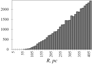
Fig. 1 shows the histogram of the distances for 38074 selected giants. The median value of of the sample is 324 pc. The giants are intrinsically brighter than O–F stars and, thus, can be investigated at a larger distance. But more importantly, the giants are much more numerous far away from the Galactic mid-plane than O–F stars. The majority of the O–F stars,which were considered by Gontcharov & Mosenkov (2017b), are within 220 pc, thus, they are located inside of the Galactic dust layer. On the other hand, the majority of the selected giants are within pc, thus, they are located behind the dust layer at high latitudes. Any conclusion about the reddening through the dust layer 111In fact, it is the dust half-layer to the North or to the South due to the position of the Sun nearly in the middle of this layer. at high latitudes would be very important because it defines a zero-point of many 3D reddening data sources. We can make such a conclusion in this study. Moreover, now we can consider the 3D reddening maps of Green et al. (2015, hereafter GSF)222http://argonaut.skymaps.info/ and Sale et al. (2014, hereafter SDB)333http://www.iphas.org/extinction/, which give poor data for pc, but reliable ones for pc (we consider only the giants with the reliable estimates).
Obviously, the larger the less precise the TGAS . Yet, photometry in many deep surveys is saturated for close and bright TGAS stars. Also, any infrared (IR) photometry is not enough sensitive for detection of the errors in reddening/extinction estimates. Therefore, we choose the Tycho-2 photometry as the only one, precise and sensitive enough (Gontcharov, 2016a), and available for all the TGAS stars under consideration (besides the Gaia band ).
Let us consider the balance of the systematic errors in the equations (1) and (2) for the selected sample. A detailed study of the TGAS giants by Gontcharov (2017b) has shown that the systematic errors for mas seem to be lower than 0.1 mas. For pc it gives mag (Parenago, 1954, p. 44). Any systematic error of or is less than 0.01 mag (Høg et al., 2000). Gontcharov & Mosenkov (2017b) have compared various estimates of reddenings/extinctions for the TGAS stars and found that even within pc their typical systematic differences are and mag, thus, representing their systematic errors. Therefore, the systematic errors of reddening/extinction dominate the balance of the systematic errors in the equations (1) and (2). Consequently, statistics of the distribution of the TGAS giants in the HR diagram would primarily reveal some systematic errors of the reddening/extinction estimates.
In this paper, for the comparison with the empirical data the proper theoretical positions of the giants in the HR diagram are calculated using the PARSEC (Bressan et al., 2012)444http://stev.oapd.inaf.it/cgi-bin/cmd and MIST (Dotter, 2016)555http://waps.cfa.harvard.edu/MIST/ isochrones and the TRILEGAL model of the Galaxy (Girardi et al., 2005) 666http://stev.oapd.inaf.it/cgi-bin/trilegal.
2 Data and results
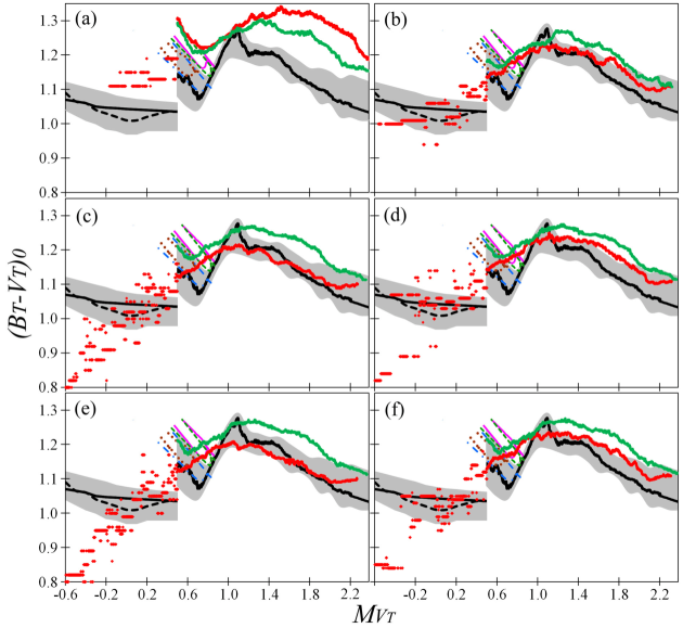
The distribution of the selected 38074 giants in the HR diagram versus 777Hereafter, the HR diagrams are rotated by 90 w.r.t. usual view because we consider the variations of some parameters with . is shown in Fig. 2 by the grey and black dots for and , respectively. Different plots in Fig. 2 show different reddening/extinction estimates used: (a) zero extinction, (b) Arenou, Grenon & Gomez (1992, hereafter AGG), (c) Schlegel, Finkbeiner & Davis (1998, hereafter SFD), (d) SFD reduced as described later (hereafter SFDR), (e) Meisner & Finkbeiner (2015, hereafter PLA), (f) PLA reduced as described later (hereafter PLAR). (g) Drimmel, Cabrera-Lavers & López-Corredoira (2003, hereafter DCL), (h) GSF, (i) Gontcharov (2009, 2012b, hereafter G12), (j) G17, (k) Chen et al. (2014, hereafter CLY)888http://lamost973.pku.edu.cn/site/data and (l) SDB. All of them, except GSF and SDB, have been described and used by Gontcharov & Mosenkov (2017b) for pc. GSF, CLY, and SDB cover only parts of the sky and provide reddening/extinction estimates only for 9010, 5483 and 2143 giants under consideration, respectively. CLY and SDB have no giants under consideration for . The DCL, GSF and SDB estimates are calculated by use of the code of Bovy et al. (2016)999https://github.com/jobovy/mwdust.
SFD and PLA are 2D (to infinity) reddening maps based on the observations of the dust emission in far-IR by COBE, IRAS, and Planck. To compare them with the 3D reddening/extinction estimates we reduce them from infinity to by use of the barometric law of the dust spatial distribution (Parenago, 1954, p. 265):
| (3) |
where is the reddening to the distance , is the reddening to infinity for the same line of sight, is the Galactic coordinate of the object along the -axis in kiloparsecs 101010To avoid confusion, the metallicity is designated hereafter as , while one of the Galactic coordinates as ., is the vertical offset of the mid-plane of the dust layer with respect to the Sun in kiloparsecs, and is the scale height of the dust layer in kiloparsecs. Following Gontcharov & Mosenkov (2017b), we accept some average values and pc. By doing so, we calculated SFDR and PLAR.
Following the PARSEC data base, we use the extinction law (i.e. the dependence of extinction on wavelength) of Cardelli, Clayton & Mathis (1989) with the fixed extinction-to-reddening ratio . With enough accuracy it can be approximated for the giants with mag by the equations:
| (4) |
and
| (5) |
where is . It is seen from these equations that for mag, exceeds by less than 15 per cent. The calculation of , and by use of the equations (2), (4) and (5) needs several iterations. We do not consider any spatial variations of the extinction law because even with for the space under consideration (Gontcharov, 2012a), these variations negligibly affect the results.
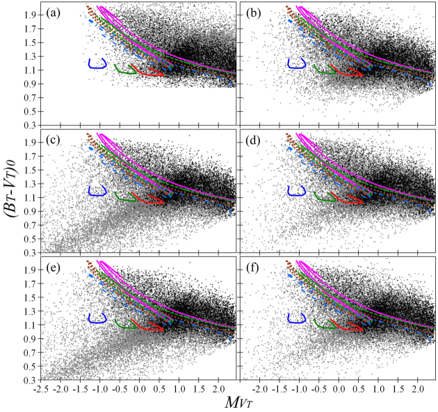
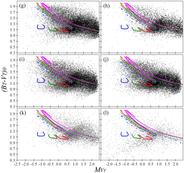
A detailed description of main kinds of the giants is given by Girardi (2016). Fig. 2 shows these kinds: the fainter part of the branch – the rightmost bulk at mag, the main clump at mag and the separation of the most luminous giants at mag into the brighter branch and the young clump 111111Girardi (2016) refer to this kind as the vertical structure, but we prefer ‘young clump’, respectively, redder and bluer than mag.
The parts of the isochrones at the branch, clump, and asymptotic branch are shown for the comparison: for 2 Gyr () and 5 Gyr () for PARSEC – the light-blue dash-dotted and green dashed curves, and MIST – the brown dotted and purple solid curves, respectively. The solar metallicity accepted in PARSEC from Bressan et al. (2012) is comparable with the protosolar metallicity accepted in MIST from Asplund et al. (2009). The relation ‘age versus metallicity’ for these isochrones is accepted on the basis of the TRILEGAL data for the sample, as discussed later. It is seen that MIST gives slightly redder isochrones than PARSEC.
Any reasonable reddening and extinction would not mix the young clump, main clump, brighter branch, and fainter branch. Yet, it is evident that the different estimates of reddening/extinction are responsible for the main difference of the plots of Fig. 2. The bulk of the stars is shifted to the right/up with lower extinction/reddening or to the left/down with higher ones. It is especially evident in plots (c), (d), (e), (f), and (l) with the estimates for from SFD, SFDR, PLA, PLAR, and SDB, respectively: plenty of giants with strongly overestimated reddening/extinction form a narrow grey bulk from the centre to the left-down corner. Initially, our sample keeps a certain level of completeness everywhere in the considered part of the HR diagram. However, the giants with considerably overestimated reddening/extinction migrate from the main clump and fainter branch making them very incomplete (for example, SFD and PLA lose more than 20 per cent of giants at the main clump and fainter branch). Moreover, in this way main clump and fainter branch contaminate the young clump. As a result, any further analysis of the distribution of the giants with the estimates for from SFD, SFDR, PLA, PLAR, and SDB is strongly biased and makes little sense. However, the distribution of the black dots in Fig. 2 shows that for these data sources do not provide such a strong overestimation of the reddening and, thus, can provide useful results.
For mag, we do not consider the brighter branch giants due to their various and poorly defined ages and metallicities. Also, due to a contamination of the young clump by the main clump and brighter branch, their has a large spread. However, the young clump giants dominate among the bluest giants. Being younger than 2 Gyr, they have a well-defined average metallicity. It is nearly equal to the solar metallicity, and lies certainly within , as follows from TRILEGAL in agreement with Haywood (2006). Moreover, their is almost independent of age, as evident from the young clump isochrones. Such PARSEC isochrones are shown in Fig. 2 by the blue, green and red solid curves at the centres of the plots, for 0.25, 0.40, and 0.63 Gyr, respectively, and . The lowest parts of these curves are the domains of the slowest evolution of the giants, thus, constituting the young clump. A lower envelope of such isochrones must fit the of any real young clump sample, if the reddening estimates are correct. Indeed, the young clump looks like a horizontal bulk of stars along this lower envelope of the isochrones in Fig. 2 (a), (b), (g), (h), (i), (j), and (k) for the zero extinction, AGG, DCL, GSF, G12, G17, and CLY, respectively. A contamination of the young clump by the main clump and brighter branch can make of the real sample slightly redder than this lower envelope of the isochrones. Yet, TRILEGAL, PARSEC and MIST suggest that somewhere within mag this contamination is so negligible that the empirical must always fit the lower envelope of the isochrones. 121212, which corresponds to , is defined by a dominant age of the young clump stars. However, it is not important because their is almost independent of age. In case of systematic overestimation/underestimation of the reddening, the of a real young clump sample is bluer/redder than this lower envelope of the isochrones. Thus, this can be a test of the reddening/extinction estimates for the young clump. Obviously, the young clump is much bluer than this lower envelope in the above mentioned cases of strong overestimation of the reddening by SFD, SFDR, PLA, PLAR, and SDB.
For mag, the sample is quite homogeneous. It has an almost Gaussian distribution by . Consequently, the average, median and mode of almost coincide. Hereafter, we consider the median as a function of , separately for (31841 giants) and (6233 giants) to reveal its variations with . Since the vast majority of the giants have , the results for all giants almost coincide with the ones for .
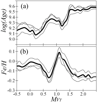
The isochrones are not enough to determine the theoretical position of the sample in the HR diagram because of some variations of the average age and metallicity of the sample over the diagram. We calculate the theoretical age and metallicity as some functions of . For this, we use TRILEGAL with the same constraints as for our sample. The calculations with the TRILEGAL default parameters from Girardi et al. (2005), but the Sun at 8 kpc from the Galactic Centre and 13 pc above the Galactic mid-plane (Gontcharov, 2008, 2011), give results shown in Fig. 4 by the solid black and grey curves, respectively, for and . The most important TRILEGAL default parameters are: initial mass function (IMF) from Chabrier (2001); binary fraction is 0.3 with mass ratios between 0.7 and 1; thin disc with squared hyperbolic secant variations of density along , exponential variations along , local calibration 55.4082 M☉ pc-2, two-step star formation rate (SFR), age versus metallicity relation (AMR) from Rocha-Pinto et al. (2000) with -enhancement as suggested by Fuhrmann (1998); as well as certain definitions of thick disc, halo and bulge. The calculations have been repeated with the parameters, which were widely varied following Girardi et al. (2005): different IMF, SFR, properties of thin disc, thick disc and halo, no or much more binaries, various extinction estimates or no extinction at all, the Sun at 7 kpc from the Galactic Centre and up to 30 pc above the Galactic mid-plane, etc.. The ranges of the results for are shown in Fig. 4 by the dashed curves.
For mag and , the calculated theoretical median as a function of is shown in Fig. 5 by the thick solid black curve, with its range due to the variations of the TRILEGAL parameters shown as the grey belt around it. This belt also includes the uncertainties of the average age and metallicity shown in Fig. 4. Such a relation ‘ versus ’ for almost coincides with the one for because, as evident from Fig. 4, the giants at have a higher age (making the giants redder) but lower metallicity (making them bluer), which compensate each other in the relation ‘ versus ’. Therefore, the relation for is not shown in Fig. 5.
For mag, the theoretical lower envelope of the above mentioned young clump isochrones from PARSEC and MIST is shown in Fig. 5 by the dashed and solid black curves, respectively. The grey belt around it shows the variations of the relation due to the accepted average metallicity within .
The data for the real giants under consideration are shown in Fig. 5 as well. Different plots in Fig. 5 show the same reddening/extinction estimates used for the stars, as in Fig. 2. For mag, the moving median over 1000 points for and 500 points for is shown by the thick red and green curves, respectively. For GSF, CLY, and SDB, 500 and 200 points are used instead of 1000 and 500, respectively, for the moving windows. For mag, the moving over 500 points for is shown by the red diamonds. Being rather young, the young clump giants are rare at .
If the TRILEGAL model with some reasonable parameters of the Galaxy is correct and if the solar metallicity is (we discuss this later), then any correct estimates of reddening/extinction would put in Fig. 5
- 1.
- 2.
- 3.
Also, the red curve almost fits the black thick curve within the grey belt for the plots (b), (d), (f), and (l) for AGG, SFDR, PLAR, and SDB, respectively. Yet, we have seen that for all of them, except AGG, this is a strongly biased result.
|
||||||||||||||||||||||||||||||||||||||||||||||||||||||||||||||||||||||||
To test the disagreement of the empirical data with TRILEGAL at mag, we show in Fig. 5 the main clump parts of the above mentioned isochrones. It is seen that the empirical data better fit the MIST (the brown dotted and purple solid curves) than PARSEC (the light blue dash-dotted and green dashed curves) isochrones. This may point out to an imperfection of TRILEGAL, because it is based on PARSEC.
One can see several cases when the empirical results agree (or almost agree) with the theoretical ones for the fainter branch and disagree for the young clump (AGG, SFD, SFDR, PLA, PLAR, G12 and SDB), and vice versa (DCL and GSF). Due to a correlation between and , the young clump giants have a slightly larger median (350 pc) than for the fainter branch (300 pc). Yet, the difference is small. It can explain the cases of (AGG, G12)/(DCL, GSF) as an overestimation/underestimation of the reddening for the most distant/nearby giants under consideration due to the adjustment of these data sources to the nearby/distant stars only. However, remaining such the cases are solely explained by the migration of the main clump and fainter branch giants to the domain of the young clump due to the overestimated reddening/extinction.
We perform two tests to estimate the agreement of the empirical and theoretical relations ‘ versus ’ for the main clump and fainter branch. The first test is the 2D Kolmogorov-Smirnov (K–S) test which determines if two data sets differ significantly. Here, we compare the empirical set of points for each map in the space ‘ versus ’ with the randomly selected points from all the variety of the used TRILIGAL models. We present the D-value (or K–S statistic) which, by definition, is the absolute maximal distance between the cumulative distribution functions of the two samples. In other words, the closer this number is to 0, the more likely it is that the two samples were drawn from the same distribution. The second test is similar to the first one but it deals with a median average curve for empirical data and the model spread which is presented by the grey belt in Fig. 5. For each extinction/reddening source, we compute the following value:
| (6) |
where is the total number of points in the median average curve, is the ordinate of the median average curve at the abscissa in the space ‘ versus ’, is an interpolation of the bottom envelope of the model spread at and is an interpolation of the top envelope of the model spread at . As such, is an averaged distance between the empirical data and the model spread.
The results are presented in Table 1. It shows that the best agreement is for G12 and G17 (formally, SFD, PLA, and SDB also give fine test results, but they have been criticized because of the strong biases).
For the young clump, the theoretical relation ‘ versus ’ is presented by the lower envelope of the isochrones, but not by a TRILEGAL simulated sample. Therefore, for the young clump the only possible test is simple: does fit the constraint , i.e. does the lowest red diamond lie within the grey belt? As seen from Fig. 5, only DCL, GSF, and G17 pass this test.
3 Discussion
|
In Fig. 5, the red curves for DCL, GSF, and CLY are not strongly biased, yet, they are located far from the grey belt. This means that these data sources generally underestimate the reddening for the giants within .
However, the most important conclusions can be made for , where all the data sources under consideration seem to give the unbiased results. As noted earlier, only the estimates of G12 and G17 fit TRILEGAL (the green curve is inside the grey belt). Table 2 contains some estimates for all the data sources at . They are the median , the minimal value of the reddening underestimation taken from the shift of the the faint branch giants (green curve) off the TRILEGAL prediction (the grey belt) along the reddening/extinction line (i.e. the value needed to put the green curve inside the grey belt), and the resulting sum of the median and . The can be considered as a median reddening estimate for by the data source and TRILEGAL. Table 2 shows that SFD, SFDR, PLA, PLAR, DCL, and GSF give the lowest median , G12 and G17 – the highest value, whereas AGG is in-between 131313AGG accepted the single value mag at behind the dust layer ( pc) due to the lack of precise measurements of the reddening/extinction at high latitudes during the construction of AGG. Yet, naturally, is almost the same for all the data sources. This leads to the conclusion that the median at is indeed mag [the median is mag following the equation (4)] and, thus, a value mag ( mag) should be added to correct the median from SFD, PLA, DCL, and GSF. Since the majority of the giants under consideration at are behind the dust layer, this correction is also needed for the SFD and PLA reddening estimates to infinity. To show this, we consider the traditionally focused values in the Galactic polar caps, for example around the northern (NGP) and southern (SGP) Galactic poles (a review of the reddening estimates at the poles is given, for example in the SFD paper). We select the giants behind the dust layer with pc. Table 3 shows that, again, SFD, SFDR, PLA, PLAR, DCL, and GSF give the lowest estimates of the median , G12 and G17 – the highest, whereas AGG is in-between. Yet, TRILEGAL supports that the median is equal to 0.06 mag at the Galactic poles.
|
The agreement or disagreement of the reddening data sources with each other is seen from their linear correlation coefficients. For they are high () only for all the pairs of SFD, SFDR, PLA, PLAR, DCL, and GSF. Also these correlation coefficients show that DCL is closer to SFD, whereas GSF is closer to PLA. For all the giants under consideration the correlation coefficients are high for all the pairs of SFD, SFDR, PLA, and PLAR (); for all the pairs of AGG, G12, and G17 (), as well as for GSF versus G17 (0.65), GSF versus G12 (0.55), GSF versus AGG (0.59) and GSF versus DCL (0.51). For the rest pairs, the correlation coefficients are lower.
This means that at some compromised reddening estimates can be found from the highly correlated estimates of G17 and GSF (remembering that AGG is based on very limited data, whereas G12 is a sister of G17 by its origin). However, at there is no such a compromise: one has to choose either a lower reddening from SFD, PLA, DCL, and GSF or a higher reddening from G17.
Besides the underestimated reddening at high latitudes, there are two other explanations for the discrepancy of the green curves and the grey belt in Fig. 5:
-
1.
TRILEGAL has not considered a reliable set of the parameters of the Galaxy, and
-
2.
the solar metallicity is instead of : with a fixed in TRILEGAL it gives a much higher for the giants under consideration and changes the TRILEGAL’s ‘ versus ’ relation greatly.
We regard the former alternative as improbable. For the latter alternative our approach sets an almost linear relation between the accepted solar metallicity and median reddening at high latitudes: corresponds to , whereas to , with, respectively, G17 or SFD, SFDR, PLA, PLAR, DCL and GSF as the best estimates. A compromise with and median is also possible. We note that the same is applicable to the previous study of the O–F stars (Gontcharov & Mosenkov, 2017b): the same increase of the accepted solar metallicity would shift the isochrones and make the DCL estimates the best.
Yet, there have been some robust arguments to accept the solar metallicity as in PARSEC (Bressan et al., 2012) or even in MIST (Asplund et al., 2009). Therefore, we should explain the suggested underestimation of the reddening at by SFD, SFDR, PLA, PLAR, DCL and GSF.
DCL and GSF are constructed with two ‘boundary conditions’: the zero reddening at the Sun, and the SFD reddening behind the dust layer. Therefore, any systematic error of SFD would appear in DCL and GSF.
Consequently, we should find an initial source of systematic errors, common for SFD and PLA. For any emission-based 2D reddening map, such as SFD or PLA, the reddening through the dust half-layer is estimated from the emission generated in this half-layer. The emission-to-reddening calibrations for SFD and PLA are based on some samples of reddened elliptical galaxies and quasars, respectively. The same for both SFD and PLA, the cosmic IR background emission from the intergalactic dust and Zodiacal IR foreground emission from the dust in the Solar system are removed at early stages of the data processing in order to obtain the emission from the Galactic dust. As a result, the median through the dust half-layer in the large low dust column density regions of the sky was set to mag in SFD and to a similar very low value in PLA. In fact, these values appear in Table 3, whereas these regions of the sky are tabulated in table 5 of the SFD paper. The uncertainty of this emission-to-reddening calibration is so high that the median mag instead of mag is quite probable. SFD attempted to use counts of galaxies (after the reddened colours of the galaxies had been used) to improve this calibration for low reddenings. They obtained a value which was at least twice larger than that which had been obtained by use of the reddening of the galaxies. Apart from other explanations, the most natural reason is that the real reddening at the regions with low reddening is indeed at least two times higher than presented in SFD.
This systematic underestimation of low reddening may appear because it is hard to distinguish the emissions from the Galactic, intergalactic and Zodiacal dust in the sky areas with low reddening/emission. The uncertainty of this distinguishing of the Galactic and Zodiacal emission may be enhanced by the orientation of the ecliptic with respect to the Galactic equator. They intersect at a large angle and near the directions to the Galactic Centre and anticentre. As a result, two parts of the Zodiacal dust belt are projected to the most dense parts of the dust layer of the Gould Belt at , and , (Gontcharov, 2012b, table 4), (see also Gontcharov, 2009, 2016b). Other parts of the Zodiacal dust belt are projected to the high latitude areas (for example, ecliptic at the longitudes and , i.e. in Leo, Virgo, Aquarius and Pisces, drops in the areas with ). In fact, in both the cases we know only the total reddening: ‘Gould Belt plus Zodiacal belt’ and ‘High latitudes plus Zodiacal belt’. Underestimation of the reddening in the Gould Belt has been a common practice. It must lead to an overestimation of the Zodiacal dust reddening and, consequently, to an underestimation of the reddening at high latitudes. This may be the case for SFD and PLA and should be tested in future studies.
Moreover, by use of the emission generated by the dust grains of one size, SFD and PLA estimate the reddening generated by the grains of another size. However, some strong variations of the extinction law far from the Galactic mid-plane, obviously, due to the variations of the distribution of grains on size have been discovered (see e.g. Gontcharov, 2012a, 2013, 2016a, 2016b). These lead to some still poorly known spatial variations of the emission-to-reddening calibration.
Finally, we shall explain the advantages of G17 as, apparently, the best reddening estimates for the local stars.
-
1.
Unlike SFD, PLA, DCL, GSF, CLY, and SDB, G17 uses the local stars, including the ones within pc. The turn-off stars are used knowingly in order to deal with a rather complete sample within and pc. However, we emphasize that G17 would be far from the best and even unreliable for distant regions of the dust layer, i.e. for with pc.
- 2.
- 3.
-
4.
Unlike the others, G17 combines the photometry and star counts to derive the reddening. The photometry is not used directly, but only to select the counted stars. This eliminates some systematic errors. It is the most important in the space with low reddening, e.g. at high latitudes, where even a small error of, say, 0.04 mag in the accepted dereddened colour becomes a reddening systematic zero-point offset. This approach allows us to obtain the estimates at high latitudes which are independent of SFD, PLA or any other emission-based map. This eliminates any error of the emission-reddening calibration, which may affect DCL, GSF, CLY, SDB and other SFD followers.
4 Conclusions
TGAS parallaxes, Tycho-2 photometry and reddening/extinction estimates from nine data sources for 38074 giants within 415 pc from the Sun have been used to compare their position in the HR diagram with the theoretical estimates based on the PARSEC and MIST isochrones and the TRILEGAL model of the Galaxy with its parameters being widely varied. The accuracy of the data allows us to reveal some considerable systematic errors of the reddening/extinction estimates as the main uncertainty in the positioning of the giants in the HR diagram.
This study confirms the same conclusions for the giants as Gontcharov & Mosenkov (2017b) made for the O–F stars. For the solar metallicity , the empirical data better fit the theoretical ones with the reddening/extinction estimates from recent 3D reddening map G17. In this case, the median reddening at high Galactic latitudes behind the dust layer is mag. Consequently, it has been considerably underestimated by the 2D reddening maps, which are based on the dust emission observations by IRAS, COBE, and Planck (SFD and PLA), and by SFD’s 3D followers (DCL and GSF). However, with a higher solar metallicity the reddening/extinction estimates from DCL and GSF become the best.
Anyway, any emission-based 2D estimates of reddening, such as SFD or PLA, even reduced to a star’s distance in assumption of the only flat layer of dust, can be wrong due to a complex distribution of the dust within 415 pc. This complexity of the local dust medium should not be described by too simplified models (DCL or AGG) or without engaging photometry of the local stars (GSF, CLY and SDB). Among the analytical models, G12 is the best, describing the local dust medium by two intersected dust layers, at the Galactic mid-plane and in the Gould Belt. Yet, the results of this study show that G12 needs a further refinement.
Acknowledgements
We thank an anonymous reviewer for useful comments. We thank Jieun Choi and Aaron Dotter for the discussion of the MIST data. AVM is partly supported by the Russian Foundation for Basic Researches (grant number 14-02-810). AVM is a beneficiary of a mobility grant from the Belgian Federal Science Policy Office. The resources of the Centre de Données astronomiques de Strasbourg, Strasbourg, France (http://cds.u-strasbg.fr) including the reddening/extinction data sources under consideration were widely used in this study. This work has made use of data from the European Space Agency (ESA) mission Hipparcos. This work has made use of data from the ESA mission Gaia (https://www.cosmos.esa.int/gaia), processed by the Gaia Data Processing and Analysis Consortium (DPAC; https://www.cosmos.esa.int/web/gaia/dpac/consortium). Funding for the DPAC has been provided by national institutions, in particular the institutions participating in the Gaia Multilateral Agreement.
References
- Arenou, Grenon & Gomez (1992) Arenou F., Grenon M., Gomez A., 1992, A&A, 258, 104 (AGG)
- Asplund et al. (2009) Asplund M., Grevesse N., Sauval A. J., Scott P., 2009, ARA&A, 47, 481
- Astraatmadja & Bailer-Jones (2016) Astraatmadja T. L., Bailer-Jones C. A. L., 2016, ApJ, 833, 119
- Bovy et al. (2016) Bovy J., Rix H.-W., Green G. M., Schlafly E. F., D.P. Finkbeiner, 2016, ApJ, 818, 130
- Bressan et al. (2012) Bressan A., Marigo P., Girardi L., Salasnich B., Dal Cero C., Rubele S., Nanni A., 2012, MNRAS, 427, 127
- Cardelli, Clayton & Mathis (1989) Cardelli J. A., Clayton G. C., Mathis J. S., 1989, ApJ, 345, 245
- Chabrier (2001) Chabrier G., 2001, ApJ, 554, 1274
- Chen et al. (2014) Chen B.-Q. et al., 2014, MNRAS, 443, 1192 (CLY)
- Dotter (2016) Dotter A., 2016, ApJS, 222, 8
- Drimmel, Cabrera-Lavers & López-Corredoira (2003) Drimmel R., Cabrera-Lavers A., López-Corredoira M., 2003, A&A, 409, 205 (DCL)
- Fuhrmann (1998) Fuhrmann K., 1998, A&A, 338, 161
- Gaia Collaboration et al. (2016a) Gaia Collaboration et al., 2016a, A&A, 595, A1
- Gaia Collaboration et al. (2016b) Gaia Collaboration et al., 2016b, A&A, 595, A2
- Girardi et al. (2005) Girardi L., Groenewegen M.A.T., Hatziminaoglou E., da Costa L., 2005, A&A, 436, 895
- Girardi (2016) Girardi, 2016, ARA&A, 54, 95
- Gontcharov (2008) Gontcharov G. A., 2008, Astron. Lett., 34, 785
- Gontcharov (2009) Gontcharov G. A., 2009, Astron. Lett., 35, 780
- Gontcharov (2011) Gontcharov G. A., 2011, Astron. Lett., 37, 707
- Gontcharov (2012a) Gontcharov G. A., 2012a, Astron. Lett., 38, 12
- Gontcharov (2012b) Gontcharov G. A., 2012b, Astron. Lett., 38, 87 (G12)
- Gontcharov (2013) Gontcharov G. A., 2013, Astron. Lett., 39, 550
- Gontcharov (2016a) Gontcharov G. A., 2016a, Astron. Lett., 42, 445
- Gontcharov (2016b) Gontcharov G. A., 2016b, Astrophysics, 59, 548
- Gontcharov (2017a) Gontcharov G. A., 2017a, Astron. Lett., 43, 471 (G17)
- Gontcharov (2017b) Gontcharov G. A., 2017b, Astron. Lett., 43, 545
- Gontcharov & Mosenkov (2017a) Gontcharov G. A., Mosenkov A. V., 2017a, MNRAS, 470, L97
- Gontcharov & Mosenkov (2017b) Gontcharov G. A., Mosenkov A. V., 2017b, MNRAS, 472, 3805
- Green et al. (2015) Green G. M. et al., 2015, ApJ, 810, 25 (GSF)
- Haywood (2006) Haywood M., 2006, MNRAS, 371, 1760
- Høg et al. (2000) Høg E. et al., 2000, A&A, 355, L27
- Meisner & Finkbeiner (2015) Meisner A. M., Finkbeiner D. P., 2015, ApJ, 798, 88 (PLA)
- Parenago (1954) Parenago P. P., 1954, A Course in Stellar Astronomy [in Russian]. GITTL, Moscow
- Rocha-Pinto et al. (2000) Rocha-Pinto H. J., Maciel W. J., Scalo J., Flynn C., 2000, A&A, 358, 850
- Sale et al. (2014) Sale S. E. et al., 2014, MNRAS, 443, 2907 (SDB)
- Schlegel, Finkbeiner & Davis (1998) Schlegel D. J., Finkbeiner D. P., Davis M., 1998, ApJ, 500, 525 (SFD)