The embedded ring-like feature and star formation activities in G35.673-00.847
Abstract
We present a multi-wavelength study to probe the star formation (SF) process in the molecular cloud linked with the G35.673-00.847 site (hereafter MCG35.6), which is traced in a velocity range of 53–62 km s-1. Multi-wavelength images reveal a semi-ring-like feature (associated with ionized gas emission) and an embedded face-on ring-like feature (without the NVSS 1.4 GHz radio emission; where 1 0.45 mJy beam-1) in the MCG35.6. The semi-ring-like feature is originated by the ionizing feedback from a star with spectral type B0.5V–B0V. The central region of the ring-like feature does not contain detectable ionized gas emission, indicating that the ring-like feature is unlikely to be produced by the ionizing feedback from a massive star. Several embedded Herschel clumps and young stellar objects (YSOs) are identified in the MCG35.6, tracing the ongoing SF activities within the cloud. The polarization information from the Planck and GPIPS data trace the plane-of-sky magnetic field, which is oriented parallel to the major axis of the ring-like feature. At least five clumps (having 740–1420 M⊙) seem to be distributed in an almost regularly spaced manner along the ring-like feature and contain noticeable YSOs. Based on the analysis of the polarization and molecular line data, three subregions containing the clumps are found to be magnetically supercritical in the ring-like feature. Altogether, the existence of the ring-like feature and the SF activities on its edges can be explained by the magnetic field mediated process as simulated by Li & Nakamura (2002).
Subject headings:
dust, extinction – HII regions – ISM: clouds – ISM: individual objects (G35.673-00.847) – ISM: Magnetic fields – stars: formation1. Introduction
In recent years, space-based infrared observations have demonstrated that the infrared structures (such as, bubbles, ring-like features, and shells) are often associated with young stellar clusters, and are commonly observed in Galactic molecular clouds (e.g. Churchwell et al., 2006, 2007; Anderson et al., 2009; Beaumont & Williams, 2010; Deharveng et al., 2010). Churchwell et al. (2006) reported that 25% of 322 mid-infrared (MIR) bubbles, distributed outside 10 of the Galactic center, are associated with known H ii regions detected at radio wavelengths. Furthermore, using the same catalog given in Churchwell et al. (2006), Deharveng et al. (2010) extended this information to 86% out of 102 bubbles through the detection of the 20 cm radio continuum emission. Hence, based on the detection/non-detection of the centimeter radio continuum emission at the sensitivity of the observed radio map, the infrared structures are seen either associated with H ii regions or devoid of H ii regions. The infrared structures associated with H ii regions are promising sites to investigate the feedback processes of massive OB stars (e.g. Deharveng et al., 2010; Kendrew et al., 2012; Thompson et al., 2012; Dewangan et al., 2016, 2017a). The photoionized gas and/or stellar winds associated with the OB stars are often considered as the major contributor for the origin of the infrared structures. Another possible mechanism responsible for the infrared structures could be supernovae explosions. On the other hand, the existence of a ring-like morphology without H ii regions is unlikely to be explained by the feedback of OB stars. The magnetic field mediated scenario has predicted the formation of ring-like features in magnetically subcritical clouds (e.g. Nakamura & Li (2002); Li & Nakamura (2002) and references therein). These authors also examined the evolution of these subcritical clouds/ring-like features, and found that a subcritical cloud fragments into multiple magnetically supercritical cores/clumps, where the birth of young stellar populations is expected. Recently, Pavel & Clemens (2012) examined the interaction of H ii region driven Galactic bubbles with the Galactic magnetic field, and found that external magnetic fields are important during the earliest phases of the evolution of H ii region driven Galactic bubbles. However, to our knowledge, a detailed observational study of the influence of the magnetic field on bubble/ring-like structures is still limited in the literature (e.g., Chen et al., 2017). Interestingly, the presence of infrared structures with H ii regions and without H ii regions in a single star-forming site can offer the possibility to explore the numerous complex physical processes involved in star formation. A detailed multi-wavelength study of such site can provide important observational evidences which can directly lead to examine the existing theoretical scenarios concerning the formation of stellar clusters and ring-like features not associated with H ii regions.
The IRAS 18569+0159/G35.673-00.847 region (hereafter G35.6) is located at a distance of 3.7 kpc (Paron et al., 2011) and is a poorly explored star-forming site. Using the radio continuum 1.4 GHz map from the NRAO VLA Sky Survey (NVSS; 1.4 GHz; Condon et al., 1998), Paron et al. (2011) studied the H ii region associated with the G35.6 site (hereafter G35.6 H ii region; see Figure 1a in this paper). Based on the MIR and radio continuum emission, the G35.6 site has an almost semi-ring-like appearance with a radius of about 15 (1.6 pc at a distance of 3.7 kpc) (Paron et al., 2011), which is associated with the main radio continuum source detected in the region (see Figures 1a and 1b). In the direction of the G35.6 H ii region, the velocity of the ionized gas is estimated to be 60.72.6 km s-1 (Lockman, 1989). Using the Galactic Ring Survey (GRS; Jackson et al., 2006) 13CO (J=10) line data, Anderson et al. (2009) computed the radial velocity of the molecular gas to be 57.1 km s-1 and designated the molecular cloud associated with the G35.6 site (hereafter MCG35.6) as D35.67-0.85. Later, using the GRS 13CO line data, Paron et al. (2011) reported the presence of a molecular shell (with a mass 104 M⊙) containing several young stellar objects (YSOs, see Figure 1b). The YSOs were identified using the Two Micron All Sky Survey (2MASS; = 1.25, 1.65, 2.2 m; Skrutskie et al., 2006) and the Galactic Legacy Infrared Mid-Plane Survey Extraordinaire (GLIMPSE; = 3.6, 4.5, 5.8, 8.0 m; Benjamin et al., 2003) photometric data sets. the majority of the 13CO gas in the molecular shell is found away from the radio continuum emission (see Figure 4 in Paron et al., 2011). In this paper, Figures 1a and 1b show the observed ionized and molecular features previously reported by Paron et al. (2011), and also reveal that the G35.6 H ii region is spatially seen in the Galactic northern side of the molecular shell. Paron et al. (2011) suggested that the G35.6 H ii region is interacting with its surrounding molecular cloud. However, the origin of the infrared and molecular structures seen in the G35.6 site still remains unexplored. The physical conditions in the G35.6 site are yet to be probed. Furthermore, the magnetic field properties in the molecular structure have not yet been studied. The investigation of dust continuum clumps and embedded young stellar clusters in the MCG35.6 is also yet to be carried out.
In this paper, to understand the ongoing physical processes and star formation activity in the G35.6 site, we present a detailed multi-wavelength study of observations from near-infrared (NIR) to radio wavelengths. The multi-wavelength data sets (including imaging, spectroscopic, and polarimetric observations) are obtained from various Galactic plane surveys. A careful investigation of these data sets allows us to probe the distribution of column density, extinction, dust temperature, ionized gas emission, kinematics of 13CO gas, plane-of-sky (POS) magnetic field, and YSOs in the MCG35.6.
This paper is structured as follows. In Section 2, we discuss the data selection. The results of our extensive multi-wavelength data analysis are presented in Section 3. The implications of our findings concerning the star formation are discussed in Section 4. Finally, our results are summarized and concluded in Section 5.
2. Data sets and analysis
In this section, we provide a brief description of the adopted multi-wavelength data sets from various Galactic plane surveys (see also Table 1). In the present work, we selected a field of 27′ 20 (29 pc 22 pc); centered at = 35.734; = 0.914.
2.1. NIR Data
We analyzed the photometric NIR data extracted from the United Kingdom Infra-Red Telescope (UKIRT) Infrared Deep Sky Survey (UKIDSS) Galactic Plane Survey (GPS; = 1.25, 1.65, 2.2 m; Lawrence et al., 2007) sixth archival data release (UKIDSSDR6plus) and the 2MASS catalogs. The UKIDSS observations (resolution ) were performed using the Wide Field Camera (WFCAM) at UKIRT. The calibration of UKIDSS fluxes was carried out using the 2MASS photometric data. In this work, we extract only reliable NIR photometric data from the catalog. To obtain reliable point sources from the GPS catalog, the conditions suggested by Lucas et al. (2008) are considered, which include the removal of saturated sources, non-stellar sources, and unreliable sources near the sensitivity limits. A SQL script (based on Lucas et al., 2008, and presented in Dewangan et al. (2015)) is especially written to implement these criteria. More information about the selection procedures of the GPS photometry can be found in Dewangan et al. (2015). We notice the UKIDSS saturation near J = 10.3, H = 11.1, and K = 9.6 mag. Hence, in our final catalog, the magnitudes of the saturated bright UKIDSS sources were obtained from the 2MASS catalog. To select good 2MASS photometric quality data, we downloaded only those sources with a photometric magnitude error of 0.1 or less in each band.
2.2. H-band Polarimetry
To obtain background starlight polarization, NIR H-band (1.6 m) linear polarimetric data (resolution ) are extracted from the Galactic Plane Infrared Polarization Survey (GPIPS; = 1.6 m; Clemens et al., 2012a) Data Release 2 (i.e. DR2). These data sets were observed with the Mimir instrument, mounted on the 1.8 m Perkins telescope, in linear imaging polarimetry mode (see Clemens et al., 2012a, for more details). To retrieve the most reliable polarimetric data, we selected the sources having , , and mag (where is the polarization percentage and is the polarimetric uncertainty).
2.3. Spitzer and WISE Data
We retrieve the photometric images and magnitudes of point sources at 3.6–8.0 m from the Spitzer-GLIMPSE survey (resolution 2). The photometric data are extracted from the GLIMPSE-I Spring ’07 highly reliable photometric catalog. We also use the Multiband Imaging Photometer for Spitzer (MIPS) Inner Galactic Plane Survey (MIPSGAL; = 24 m; Carey et al., 2005) 24 m image (resolution 6) and the photometric magnitudes of point-like sources at 24 m (from Gutermuth & Heyer, 2015).
The archival Wide Field Infrared Survey Explorer (WISE111WISE is a joint project of the University of California and the JPL, Caltech, funded by the NASA; = 3.4, 4.6, 12, 22 m; Wright et al. (2010)) image at MIR 12 m (spatial resolution 6) is also retrieved.
2.4. Herschel Data
To probe the far-infrared (FIR) and sub-millimeter (sub-mm) emission, Herschel continuum maps at 70 m, 160 m, 250 m, 350 m, and 500 m are obtained from the Herschel Space Observatory (Pilbratt et al., 2010; Poglitsch et al., 2010; Griffin et al., 2010; de Graauw et al., 2010) data archives. Level2-5 processed Herschel images were downloaded through the Herschel Interactive Processing Environment (HIPE, Ott, 2010). These observations are part of the Herschel Infrared Galactic Plane Survey (Hi-GAL; = 70, 160, 250, 350, 500 m; Molinari et al., 2010) project. The plate scales of 70, 160, 250, 350, and 500 m images are 3′′.2, 3′′.2, 6′′, 10′′, and 14′′ pixel-1, respectively. The beam sizes of the Herschel images are 58, 12, 18, 25, and 37 for 70, 160, 250, 350, and 500 m, respectively (Poglitsch et al., 2010; Griffin et al., 2010). The Herschel images at 70–160 m are calibrated in Jy pixel-1, while the units of images at 250–500 m are MJy sr-1.
Following the methods presented in Mallick et al. (2015), the Herschel temperature and column density maps are generated using the Herschel continuum images. These maps are produced from a pixel-by-pixel spectral energy distribution (SED) fit with a modified blackbody to the cold dust emission at Herschel 160–500 m (see also Dewangan et al., 2015).
A brief step-by-step explanation of the adopted procedures is as follows. Before the SED fit, the 160–350 m images are converted into the same flux unit (i.e. Jy pixel-1) and convolved to the lowest angular resolution of the 500 m image (37). Furthermore, we regrid these images to the pixel size of the 500 m image (14). These steps are carried out using the plug-in “Photometric Convolution” and task “Convert Image Unit” available in the HIPE software. Next, the sky background flux level was computed to be 0.211, 0.566, 1.023, and 0.636 Jy pixel-1 for the 500, 350, 250, and 160 m images (size of the selected featureless dark region 49 64; centered at: = 35.208; = 1.47), respectively.
In the final step, a modified blackbody is fitted to the observed fluxes on a pixel-by-pixel basis to obtain the temperature and column density maps (see equations 8 and 9 in Mallick et al., 2015). The fitting is performed using the four data points for each pixel, retaining the dust temperature (Td) and the column density () as free parameters. In the analysis, we use a mean molecular weight per hydrogen molecule () of 2.8 (Kauffmann et al., 2008) and an absorption coefficient () of 0.1 cm2 g-1, including a gas-to-dust ratio ( ) of 100, with a dust spectral index () of 2 (see Hildebrand, 1983). We further discuss these Herschel maps in Section 3.5.
2.5. Planck 353 GHz data
To obtain dust polarized emission, we use the Planck222Planck (http://www.esa.int/Planck) is a project of the European Space Agency (ESA) with instruments provided by two scientific consortia funded by ESA member states and led by Principal Investigators from France and Italy, telescope reflectors provided through a collaboration between ESA and a scientific consortium led and funded by Denmark, and additional contributions from NASA (USA). polarization data ( = 353 GHz; Planck Collaboration IX, 2014) observed with the High Frequency Instrument (HFI) at 353 GHz, where the dust polarized emission is brightest. The Planck intensity and polarization (Stokes parameters , , and ) sky maps are obtained from the 2015 release of Planck legacy archive (Planck Collaboration I, 2016a). The procedures of map-making, calibration, and correction of systematic effects are described in Planck Collaboration VIII (2016b). We smooth the maps from an initial angular resolution of 4′.9 to 6 to increase the signal-to-noise ratio and to minimize beam depolarization effects. The contribution from the cosmic microwave background (CMB) emission is very minimum and has been ignored. The intensity and polarization maps are converted from temperature scale of to MJy sr-1 using the unit conversion and color correction factor of 246.543 (Planck Collaboration IX, 2014). The intensity map is also subtracted from the Galactic zero level offset of 0.0885 MJy sr-1 (Planck Collaboration VIII, 2016b). The linear polarization of dust emission integrated along the line-of-sight is measured from the Stokes parameters , , and as:
| (1) |
| (2) |
| (3) |
where is the polarization intensity, is the percentage of dust polarization fraction, and is the polarization angle. The Planck Stokes parameters are in the HEALPix (Górski et al., 2005) convention having the angle = 0 toward the north Galactic pole and positive toward the west (clockwise). We use the IAU convention (Hamaker & Bregman, 1996) by changing the Planck Stokes map to negative so that the polarization angle is measured anticlockwise relative to the north Galactic pole. Since the noise in the maps introduces a positive bias on the measured polarization, we debias the polarization following the method given in Plaszczynski et al. (2014), and using the full available noise covariance matrix.
2.6. 13CO (J=10) Line Data
In our selected target region, we probe the molecular gas content in the MCG35.6 using the GRS 13CO (J=10) line data. The GRS line data have a velocity resolution of 0.21 km s-1, an angular resolution of 45 with 22 sampling, a main beam efficiency () of 0.48, a velocity coverage of 5 to 135 km s-1, and a typical rms sensitivity (1) of K (Jackson et al., 2006).
2.7. Radio Centimeter Continuum emission
To trace the ionized gas emission in the G35.6 site, we use the NVSS 1.4 GHz continuum map. The survey covers the sky north of = 40 at 1.4 GHz with a beam of 45 and a nearly uniform sensitivity of 0.45 mJy/beam (Condon et al., 1998). The Coordinated Radio and Infrared Survey for High-Mass Star Formation (CORNISH; Hoare et al., 2012) 5 GHz (6 cm) radio continuum data (beam size 15) are also utilized in the present work.
3. Results
3.1. Physical environment of G35.6
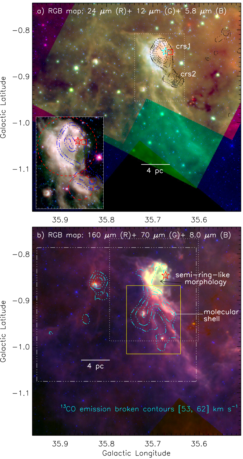
The investigation of the ionized gas, dust (cold and warm), and molecular emission enables us to probe the embedded structures present in a given star-forming region. In Figure 1, we show the spatial distribution of dust (warm and cold), molecular gas, and ionized gas toward the G35.6 site. The radio continuum data trace the ionized gas emission, while the sub-mm data are sensitive to the cold dust. The MIR and FIR data trace the warm dust. Figure 1a is a three-color composite image made using the MIPSGAL 24 m in red, WISE 12 m in green, and GLIMPSE 5.8 m in blue. The color composite image is overlaid with the NVSS radio continuum emission at 1.4 GHz, revealing two compact radio sources (designated as crs1 and crs2). These radio sources, crs1 and crs2, were previously referred to as NVSS 185929+020334 and NVSS 185938+020012, respectively (e.g., Condon et al., 1998; Paron et al., 2011). One of the radio sources, crs1 is seen near the location of IRAS 18569+0159. The inset on the bottom left shows a zoomed-in view of the two radio continuum peaks using the WISE and Spitzer images (12 m (red), 8.0 m (green), and 5.8 m (blue); see Figure 1a). There is an extended emission seen at 5.8–12 m. In the literature, it has been reported that the ionized gas and the MIR/FIR emission (at 12/24/70 m) are seen systematically correlated in H ii regions (e.g. Deharveng et al., 2010; Paladini et al., 2012). In the vicinity of crs1 and crs2, infrared features are also noticeably observed (see broken circles in the inset). It is also known that the 5.8–12 m bands contain various polycyclic aromatic hydrocarbon (PAH) features at 6.2, 7.7, 8.6, and 11.3 m (including the continuum). The presence of PAH features can be used to trace photodissociation regions (or photon-dominated regions, or PDRs) and enables us to infer the impact and influence of the H ii regions on their surroundings (see broken circles in the inset). The detection of the CORNISH 5 GHz continuum emission is also indicated by a square in Figure 1a (see also the inset). The quantitative calculations using these radio data are performed in Section 3.3.
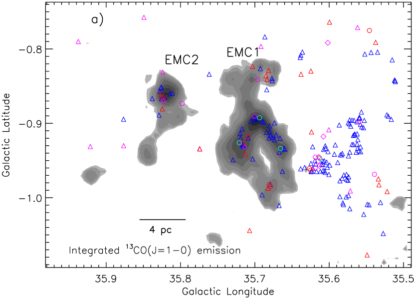
Figure 1b shows a three-color composite image made using the Herschel 160 m (in red), Herschel 70 m (in green), and GLIMPSE 8.0 m (in blue) images. The composite image is overlaid with the 13CO molecular gas emission. In the direction of our selected region, the 13CO emission traces the molecular gas in the velocity range of 53–62 km s-1. The distribution of 13CO also depicts a molecular shell. Furthermore, in the composite map, an almost semi-ring-like feature is prominently observed. As mentioned earlier, these ionized and molecular features are already known in the literature (e.g. Paron et al., 2011). In the composite map, a small dotted box (in white) highlights the area investigated by Paron et al. (2011). Additionally, a molecular condensation is also observed in the Galactic eastern side of the molecular shell (see Figure 1b). A detailed analysis of the molecular and ionized features is presented in Sections 3.2 and 3.3, respectively.
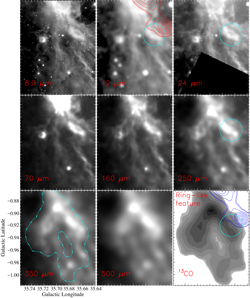
Most of the molecular gas is spatially found in the Galactic southern side of the radio source, crs1 (see a yellow box in Figure 1b). A zoomed-in multi-wavelength view of this area (selected field 7 9 (or 7.8 pc 10.3 pc)) is presented in Figure 2. The images are shown at 8.0 m, 12 m, 24 m, 70 m, 160 m, 250 m, 350 m, 500 m, and integrated intensity map of 13CO (J=10) from 53 to 62 km s-1. Note that an almost ring-like feature is evident in the integrated 13CO intensity map and the Herschel sub-mm images (at 250–500 m). The central cavity of the molecular emission coincides with a dark region in the infrared images, suggesting that there are no stars and dust condensations. The integrated 13CO intensity map and the image at 12 m are also superimposed with the NVSS 1.4 GHz emission, indicating that the ionized gas emission is not seen inside the ring-like feature. However, the radio source, crs2 is spatially seen at the most north-western section of the ring-like feature. In the closest vicinity of crs2, within a circle with a radius of 1.25 pc, we find a small feature seen in the infrared and sub-mm images (see a circle in Figure 2 and also the inset in Figure 1a). The feature is resolved in the images below at 100 m, while, in the longer wavelength images ( 100 m), it becomes a part of the ring-like feature. The energetic and feedback of the massive star associated with crs2 seems to influence this feature (see Section 3.4 for more details).
The analysis of multi-wavelength images reveals the presence of a semi-ring-like feature (associated with the radio source crs1) and an embedded ring-like feature (without detectable ionized gas emission), at the sensitivity of the observed NVSS radio map (1 0.45 mJy beam-1) in the G35.6 site. The presence of a ring-like feature in G35.6 is an excellent example for comparing with theoretical models, since observationally it is scarce and difficult to find such features with a high degree of geometrical and projectional symmetry. Overall, with the help of Figures 1, and 2, we have obtained a pictorial multi-wavelength view of the G35.6 site.
3.2. Molecular gas properties in MCG35.6
In this section, we present a kinematic analysis of molecular gas in the MCG35.6. Note that previously, Paron et al. (2011) also analyzed the GRS 13CO data and presented the integrated GRS 13CO intensity map and velocity channel maps mainly toward the G35.6 H ii region (see a small dotted box in Figure 1b). In the present work, we have carefully examined the gas distribution in the direction of our selected target field, and have also performed the position-velocity analysis of molecular gas, which was lacking in the earlier published work.
3.2.1 Velocity profiles and molecular cloud
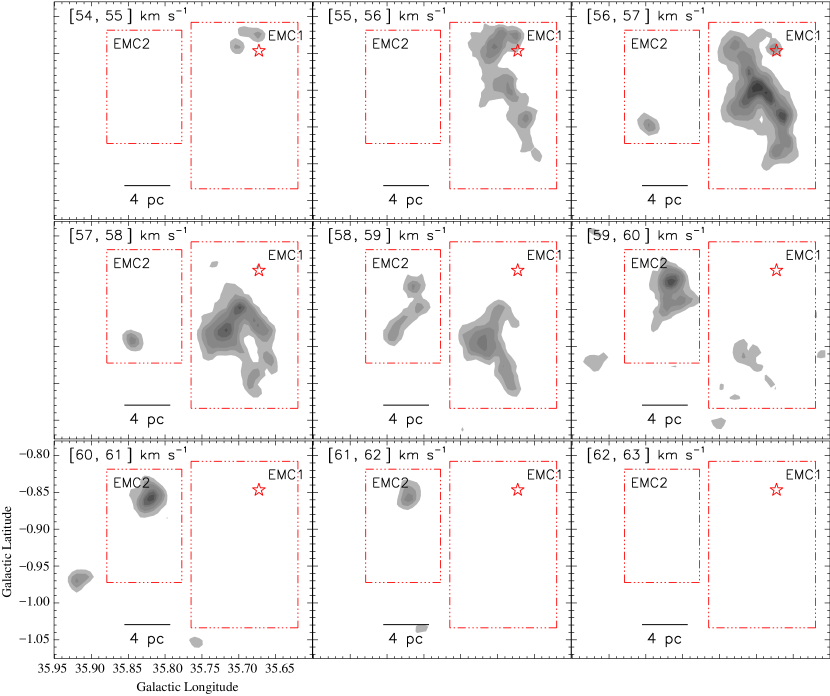
The integrated GRS 13CO (J=10) velocity channel maps (at intervals of 1 km s-1) are presented in Figure 3, which cover the velocity range from 54 to 63 km s-1. The channel maps reveal two spatially distinct molecular structures, which can also be referred to as extended molecular condensations (EMCs). The first one (EMC1) is seen in a velocity range from 55 to 60 km s-1, and appears to be associated with the radio continuum emission. It has an extended morphology showing an almost ring-like feature at a velocity of 57–58 km s-1 (see also Figure 2). The second structure (EMC2) appears at velocities from 56 to 62 km s-1. At low velocities it is compact and peaks at the coordinates l = 35.85, b = 0.94, while it extends to the north when moving to high velocities having the red-shifted peak at the coordinates (l = 35.85, b = 0.85).
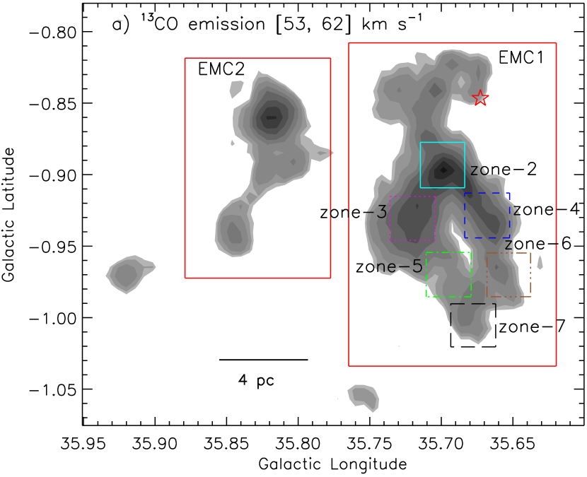
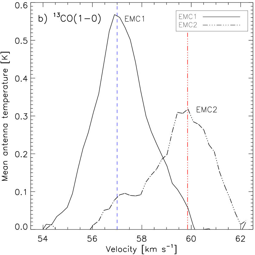
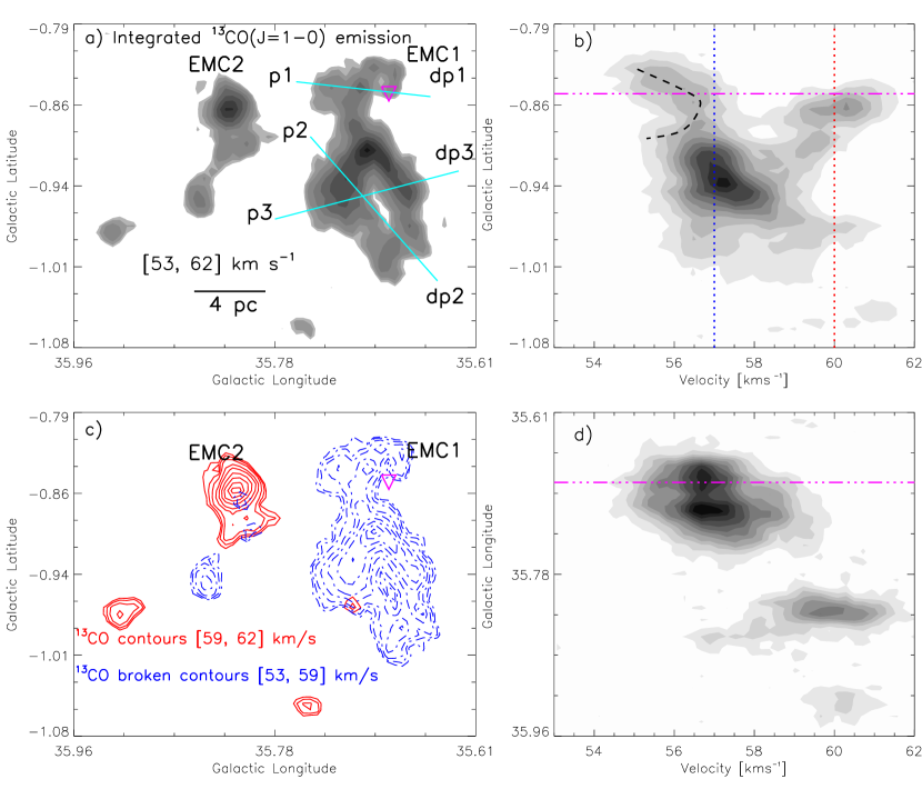
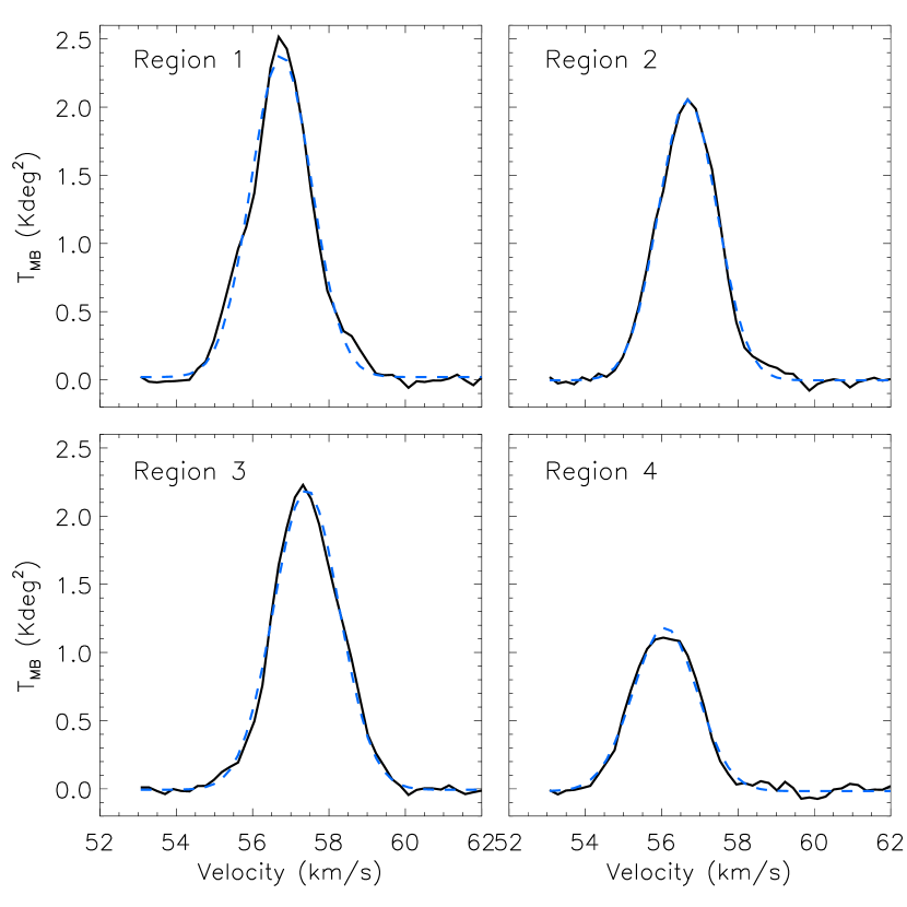
Figure 4a shows an integrated intensity map of 13CO (J = 1-0) from 53 to 62 km s-1, revealing clearly both the molecular condensations, EMC1 and EMC2 (see also Figure 3). In the integrated 13CO map, the ring-like feature is evident at the Galactic southern side of EMC1. In Figure 4b, we show the observed 13CO (J=1–0) spectral profiles in the direction of EMC1 and EMC2 (see respective box in Figure 4a). In the direction of EMC1, the velocity peak is seen at 57 km s-1, while the velocity peak toward EMC2 is found at 60 km s-1. These profiles further confirm the presence of two molecular cloud components in our selected site. Figure 4c shows the observed 13CO (J=1–0) spectra in the direction of six fields associated with the ring-like feature (i.e. zone-2 to zone-7; see broken boxes in Figure 4a). Each spectrum is constructed by averaging the area highlighted by a box in Figure 4a. In Figure 4c, the velocity peaks in the profiles are varying between 57 and 58.5 km s-1. Based on the comparison of velocity peaks in six profiles, one can find evidence of gas motion in the molecular feature. One can note that zones 2, 4, and 6 trace the west segment of the ring-like feature, while zones 3, 5, and 7 depict the eastern side. The velocity peaks seen in the direction of zones 2, 4, and 6 have very similar values, while the velocity peaks observed in the direction of zones 3, 5, and 7 have slightly different values, and also have noticeable higher values (i.e. red-shifted) than the ones seen toward the zones 2, 4, and 6 (see Figure 4c). This result also indicates the existence of a velocity spread across the ring-like feature (see also Section 3.2.2).
Considering these results and the spatial distribution of molecular gas, the ring-like feature has an ellipsoid shape along the line of sight. In 3D, we assume that this molecular feature has a spherical oblate morphology.
3.2.2 Position-velocity diagrams
To further study the molecular gas distribution in the direction of our selected target field, in Figure 5, we present the integrated 13CO intensity map and the position-velocity diagrams.
In Figure 5a, we show the molecular 13CO (J = 1–0) gas emission in the direction of the G35.6 site, which is the same as shown in Figure 4a. In Figures 5b and 5d, we present the Galactic position-velocity diagrams of 13CO emission. The 13CO emission is integrated over the longitude range and latitude range in the latitude-velocity diagram (see Figure 5b) and longitude-velocity diagram (see Figure 5d), respectively. The position-velocity diagrams also trace both the molecular components along the line of sight. A molecular component associated with the G35.6 H ii region is seen in a velocity range of 53–59 km s-1 (i.e. EMC1), while the other molecular component is observed at 59–62 km s-1 (i.e. EMC2) (see also Section 3.2.1). In Figure 5c, we present the spatial distribution of molecular gas associated with these two molecular components. The figure also reveals that these two components (i.e., EMC1 and EMC2) are clearly separated in both space and velocity, and are unrelated molecular clouds. Hence, our present work is mainly focused toward EMC1.
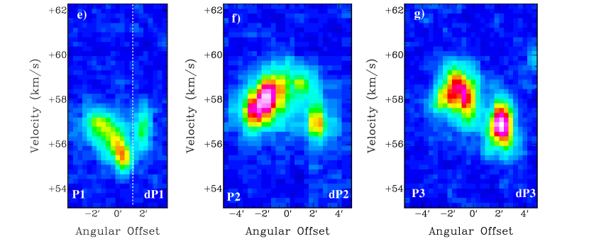
Figures 5e, 5f, and 5g show the position-velocity diagrams of 13CO along the axis “p1–dp1”, “p2–dp2”, and “p3–dp3”, respectively. The axis “p1–dp1” is selected toward the radio source crs1, while the other two axes are chosen toward the ring-like feature. In the direction of crs1/the semi-ring-like feature, the position-velocity diagrams show hints of an almost inverted C-like structure (see Figure 5e and also a black dashed curve in Figure 5b). In the velocity space, the detection of an inverted C-like or arc-like structure indicates the presence of a bubble/shell (Arce et al., 2011). Hence, in the direction of the semi-ring-like feature, our analysis suggests the presence of an expanding shell with an expansion velocity333In the velocity space, the expansion velocity corresponds to half of the velocity range for the inverted C-like structure. of the gas to be 1.2 km s-1. The position of crs1 is highlighted in Figures 5a– 5e, and nearly appears at the center of the inverted C-like structure (see Figures 5b and 5e).
In Figures 5b and 5d, a noticeable velocity spread is also found, where the majority of molecular gas is observed, indicating the gas movement in the ring-like feature (see also Figure 4c). In the direction of the ring-like feature, Figures 5f and 5g further reveal the observed velocity structures. A velocity spread across the molecular feature is also evident in the diagrams. In the velocity space, two velocity peaks (i.e. 57 and 58 km s-1) are seen, likely connected by diffuse gas and therefore suggesting the presence of a single structure with velocity gradients. Higher spectral and angular resolution data can better resolve the structure and the kinematics of the gas in the ring-like structure. As mentioned earlier, there is no ionized gas emission seen inside the ring-like feature, hence the observed velocity spread may not be explained by an H ii region.
3.3. Ionized gas properties
In this section, we investigate the spectral types of the powering candidates responsible for the compact radio sources (i.e., crs1 and crs2). We have computed the number of Lyman continuum photons () for each compact radio source using the integrated flux density following the equation of Matsakis et al. (1976). The “clumpfind” IDL program (Williams et al., 1994) can be employed in a given radio continuum map to compute the integrated flux densities. Using the 1.4 GHz map, we estimated the integrated flux densities (radii) equal to 160.7 mJy (1.8 pc) and 58.8 mJy (1.25 pc) for compact radio sources, crs1 and crs2, respectively. The equation of is defined by Matsakis et al. (1976):
| (4) |
where Sν is the measured total flux density in Jy, D is the distance in kpc, Te is the electron temperature, and is the frequency in GHz. These calculations were carried out for a distance of 3.7 kpc and for the electron temperature of 10000 K. Finally, we find (or log) to be 1.7 1047 s-1 (47.24) and 6.3 1046 s-1 (46.8) for compact radio sources, crs1 and crs2, respectively. Each compact radio source appears to be associated with a single ionizing star of spectral type B0.5V–B0V (see Table II in Panagia, 1973, and also Smith et al. (2002)).
Paron et al. (2011) utilized a total flux density of 0.86 Jy at 2.7 GHz for G35.6, and estimated to be 1.0 1048 s-1. The 2.7 GHz continuum data, as part of the Bonn 11 cm survey, were taken with the Effelsburg 100 meter telescope, and have an angular resolution of 4′.3, and 50 mK rms sensitivity (Reich et al., 1984). Note that the 2.7 GHz continuum data have a much coarser resolution compared to the NVSS 1.4 GHz continuum map. Hence, the total 2.7 GHz flux density appears to contain radio emission contribution from both the radio sources, crs1 and crs2. Using the NVSS 1.4 GHz data, the fluxes of crs1 and crs2 added together result in about 220 mJy. This value is much smaller than the total flux density at 2.7 GHz for G35.6, indicating that the Effelsburg map might be detecting some extended emission that is filtered out by the interferometer in the NVSS survey. Furthermore, Paron et al. (2011) used the 1.4 GHz data for the compact radio source, crs2 (or NVSS 185938+020012), and computed to be 0.6 1047 s-1, which is consistent with our estimates. Using these values of , we find at our end that these estimates correspond to a single ionizing star of spectral type O9V-O8.5V and B0.5V-B0V for G35.6 and crs2 (see Martins et al. (2005), Panagia (1973), and Smith et al. (2002), for theoretical values), respectively. However, Paron et al. (2011) reported the spectral type of the ionizing star of G35.6 to be between O7.5V and O9V, considering errors of about ten percent in both the distance and the radio continuum flux at 2.7 GHz. They also reported the spectral type of the ionizing star of crs2 to be later than O9.5V star. These authors have not computed the radio spectral type for crs1. Based on our independent calculations using the 1.4 GHz data, it appears that the spectral types of radio sources reported by Paron et al. (2011) are overestimated. Hence, spectroscopic observations will be needed to confirm the spectral types of the exciting stars. Using the photometric data, Paron et al. (2011) suggested that a source J18592786+0203057 is the more likely exciting-star candidate of G35.6, while two objects J18593584+0200579 and J18593556+0200488 could be the powering source candidates of crs2 (see Table 1 in their paper). Furthermore, in the G35.6 site, a point-like source is also observed in the CORNISH 5 GHz continuum map (beam size 15), and is referred to as G035.6624-00.8481 in the CORNISH 5 GHz compact source catalog (Purcell et al., 2013). The position of this radio source is indicated by a square in Figure 1a, and appears about 1′.4 away from the peak position of crs1. However, in the direction of crs1, the CORNISH source is seen well within the NVSS radio emission contours (see Figure 1a). Purcell et al. (2013) also computed a total integrated flux density equal to 5.43 mJy for the CORNISH source (having an angular size of 1′.5). With the help of equation 4, we find that the observed 5 GHz flux (having log 45.82 s-1) of G035.6624-00.8481 can be explained by a single ionizing star of spectral type B1V–B0.5V, which is nearly consistent with the spectral type of crs1 estimated using the NVSS 1.4 GHz data.
With the estimates of and radii of the H ii regions (RHII), we have also computed the dynamical age (tdyn) of each compact radio source. The age of the H ii region can be obtained at a given radius RHII, using the following equation (Dyson & Williams, 1980):
| (5) |
where cs is the isothermal sound velocity in the ionized gas (cs = 11 km s-1; Bisbas et al. (2009)), RHII is previously defined, and Rs is the radius of the Strömgren sphere (= (3 /4)1/3, where the radiative recombination coefficient = 2.6 10-13 (104 K/T)0.7 cm3 s-1 (Kwan, 1997), is defined earlier, and “n0” is the initial particle number density of the ambient neutral gas. Adopting a typical value of n0 (=103 cm-3), the dynamical ages of the compact radio sources, crs1 and crs2 are estimated to be 0.5 and 0.35 Myr, respectively. Note that the H ii regions are assumed to be uniform and spherically symmetric. Recently, Peters et al. (2010) indicated that the dynamical process of the H ii regions could be more complex, and dynamical ages can not be estimated accurately with the assumptions of uniform and spherically symmetric. Hence, the derived dynamical ages of the H ii regions can be considered as the indicative values.
The radio continuum map at 1.4 GHz is also utilized to obtain the electron density () of the ionized gas. The formula of “” is presented in Panagia & Walmsley (1978) under the assumption that the H ii region has a roughly spherical geometry:
| (6) |
In the equation above, Sν, , and D are defined as in Equation 4, is the angular radius in arcminutes, and
Considering the values of Sν and for each of the compact radio sources, the values of are computed to be 30 and 32 cm-3 for crs1 and crs2, respectively. Using the CORNISH 5 GHz data, we have also computed the value of to be 9250 cm-3 for G035.6624-00.8481. Hence, the CORNISH 5 GHz observations suggest the presence of an ultracompact H ii region in the G35.6 site. The calculation was carried out for D = 3.7 kpc and Te = 10000 K. Note that the electron density of these two radio sources estimated using the 1.4 GHz data appears smaller than the one measured assuming optically thin emission. Therefore, radio continuum observations with radio interferometers at different frequencies can be helpful to better determine the SED of the H ii regions and obtain a more accurate measurement of the properties of the H ii regions and the spectral type of the ionizing stars (e.g. Panagia & Felli, 1975; Olnon, 1975; Kurtz, 2005; Sánchez-Monge et al., 2013).
3.4. Feedback effect of massive stars
Our radio data analysis reveals that each compact radio source is excited by a radio spectral type of B0.5V star (see Section 3.3). The radio continuum peak of crs1 is found to be associated with the semi-ring-like structure (see Figure 1a). It is also observed that the radio source crs2 is located toward the north-western part of the ring-like feature (see Figure 2). To explore the feedback of the B0.5V star in its vicinity, we infer the values of three pressure components (i.e., pressure of an H ii region (), radiation pressure (), and stellar wind ram pressure ()) driven by a massive star. The equations of these pressure components (, , and ) are given below (e.g. Bressert et al., 2012):
| (7) |
| (8) |
| (9) |
where , , and are previously defined, = 0.678 (in the ionized gas; Bisbas et al., 2009), is the hydrogen atom mass, is the mass-loss rate, Vw is the wind velocity of the ionizing source, is the bolometric luminosity of the source, and Ds is the projected distance from the position of the B0.5V star where the pressure components are evaluated. The pressure components driven by massive stars are estimated at angular sizes of the radio sources (i.e. almost twice the radii of crs1 and crs2). Using the 1.4 GHz map, we obtained the radii equal to 1.8 pc and 1.25 pc for radio sources, crs1 and crs2, respectively. Hence, we have computed the pressure components at Ds = 3.5 pc (2.5 pc) for crs1 (crs2).
In the calculations, we have adopted the values of = 19950 L⊙ (Panagia, 1973), = 2.5 10-9 M⊙ yr-1 (Oskinova et al., 2011), and = 1000 km s-1 (Oskinova et al., 2011), for a B0.5V star. With the help of equations 4, 5, and 6, in the case of crs1 with Ds = 3.5 pc, we find 1.5 10-11 dynes cm-2, 1.7 10-12 dynes cm-2, and 1.1 10-14 dynes cm-2. This also gives a total pressure ( = + + ) driven by a massive star to be 1.7 10-11 dynes cm-2. Similarly, in the case of crs2 with Ds = 2.5 pc, we obtain 1.5 10-11 dynes cm-2, 3.4 10-12 dynes cm-2, 2.1 10-14 dynes cm-2, and 1.8 10-11 dynes cm-2. These calculations suggest that in both cases, the pressure of the H ii region is relatively higher than the radiation pressure and the stellar wind pressure. Note that in both the cases, is comparable to the pressure of a typical cool molecular cloud ( 10-11–10-12 dynes cm-2 for a temperature 20 K and particle density 103–104 cm-3) (see Table 7.3 of Dyson & Williams, 1980). This implies that the edges of the semi-ring and ring-like features are not wiped out by the impact of the ionized gas. Our analysis further suggests that the semi-ring-like morphology can be explained due to the ionizing feedback from the B0.5V type star, and the most north-western section of the ring-like feature (see a circle in Figure 2) is likely to be affected by the radio source crs2. Further observations of PDR tracers (e.g. Hollenbach & Tielens, 1997; Treviño-Morales et al., 2016; Goicoechea et al., 2017) can better confirm the influence of crs2 on the molecular gas of the ring-like feature.
3.5. Temperature and column density maps of G35.6
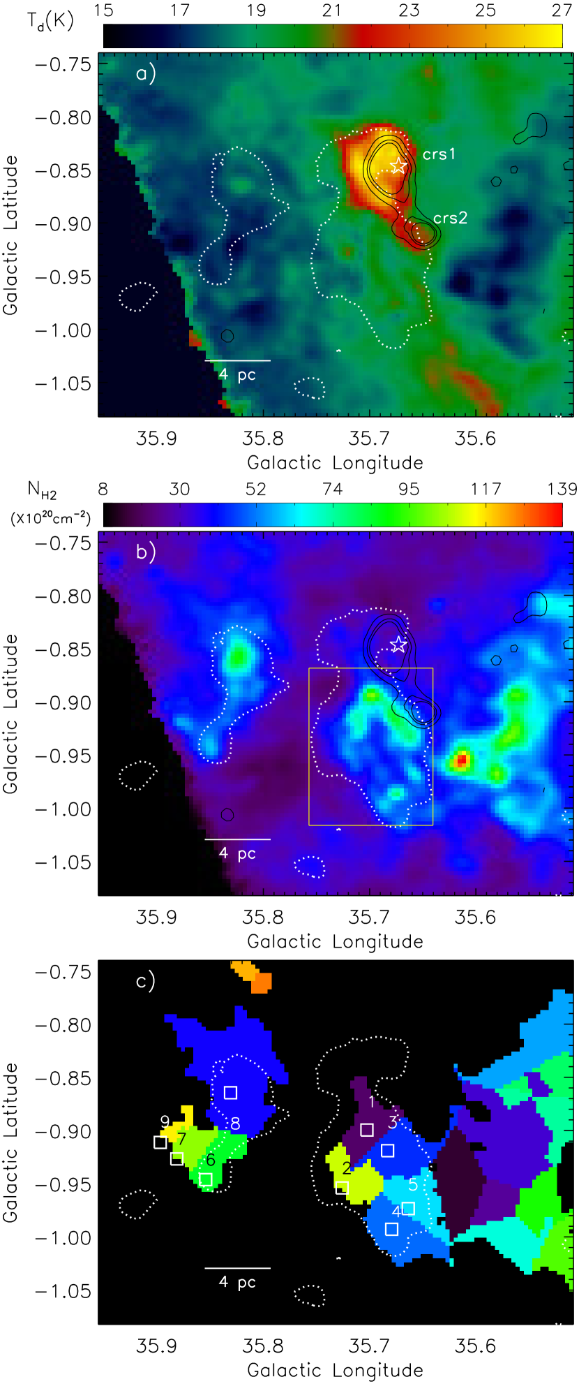
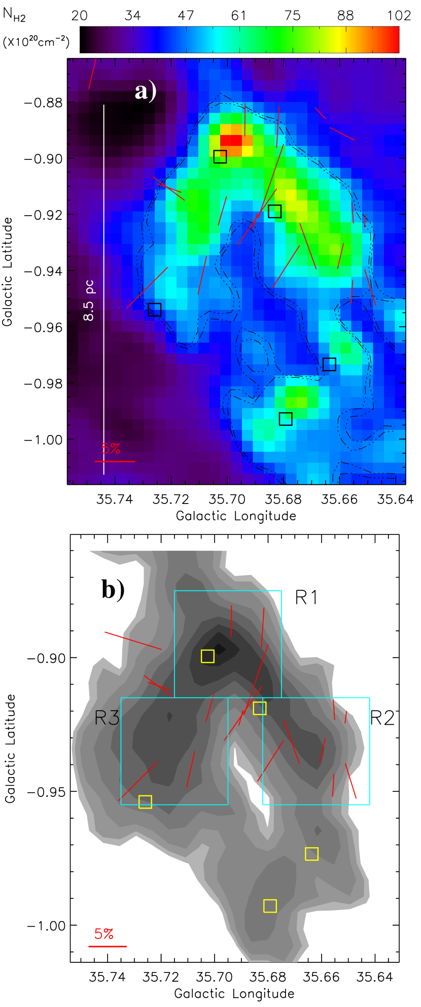
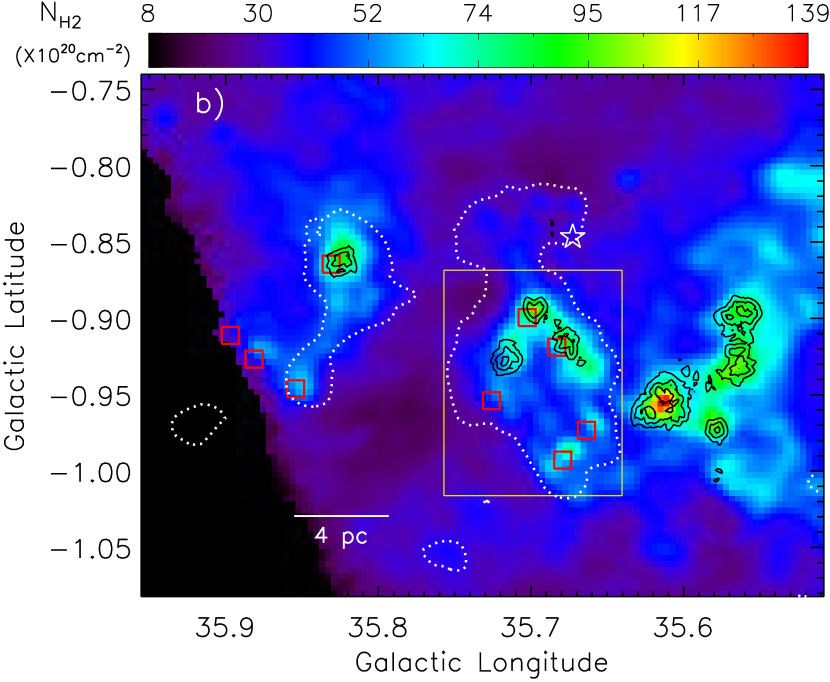
In this section, to probe the embedded structure and dust condensations, we present the Herschel temperature and column density maps (resolution 37) of the MCG35.6. The temperature and column density maps are shown in Figures 6a and 6b, respectively. The procedures for producing the Herschel temperature and column density maps were described in Section 2.4.
In the Herschel temperature map, the compact radio continuum sources (i.e., crs1 and crs2) are seen associated with warmer emission ( 22-27 K; see Figure 6a), confirming the influence of the radio continuum sources on the dense gas as discussed in Section 3.4. In the Herschel column density map, several condensations are observed in the MCG35.6 (see Figure 6b). The “clumpfind” IDL program is executed to identify the clumps and to estimate their total column densities. Several column density contour levels were used as an input parameter for the “clumpfind”, and the lowest contour level was considered at 3. Nine clumps are found in the MCG35.6 and are highlighted in Figure 6c. Furthermore, the boundary of each clump is also presented in Figure 6c. With the knowledge of the total column density of each clump, we have also determined the mass of each Herschel clump using the following equation:
| (10) |
where is assumed to be 2.8, is the area subtended by one pixel, and is the total column density. The mass of each Herschel clump is provided in Table 2. The table also gives an effective radius and a peak column density of each clump, which are extracted from the clumpfind algorithm. The clump masses vary between 175 M⊙ and 3390 M⊙. The peak column densities of these clumps vary between 4.2 1021 cm-2 (AV 4.5 mag) and 10 1021 cm-2 (AV 10.5 mag) (see Table 2 and also Figure 2b). Here, we used a relation between optical extinction and hydrogen column density (i.e. ; Bohlin et al., 1978). We find that the EMC1 contains five Herschel clumps (i.e., nos. 1, 2, 3, 4, and 5) and the total mass of these five clumps is 5535 M⊙. Interestingly, the ring-like feature embedded within EMC1 is also traced in the Herschel column density map (see a solid yellow box in Figure 6b). Furthermore, at least five clumps (i.e., nos. 1, 2, 3, 4, and 5) appear to be nearly regularly spaced along the ring-like feature. The mean separation between the clumps is computed to be 164′′.666′′.5 (or 2.951.20 pc). One can also find at least three Herschel clumps (i.e., nos. 6, 7, and 8) toward EMC2.
3.6. Polarimetric properties of MCG35.6
In this section, we analyze the background starlight polarization from the GPIPS and the dust polarized emission from the Planck, to study the magnetic field morphology and properties. The POS magnetic field direction can be inferred through the polarization observations from and due to dust grains. Polarization of radiation emitted by spinning dust grains is parallel to their long axis and the projected field direction can be obtained through the polarization vectors rotated by 90 degrees. The physical process (i.e. radiative torque mechanism) concerning the alignment of dust gains and magnetic field is described in Dolginov & Mitrofanov (1976) (see also Lazarian, 2007; Andersson et al., 2015). Using the polarization vectors of background stars, one can also obtain the field direction in the POS parallel to the direction of polarization (Davis & Greenstein, 1951). Polarization of background starlight can be explained due to the dichroism by non-spherical dust grains.
3.6.1 Magnetic field structure
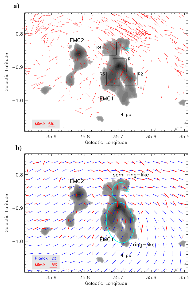
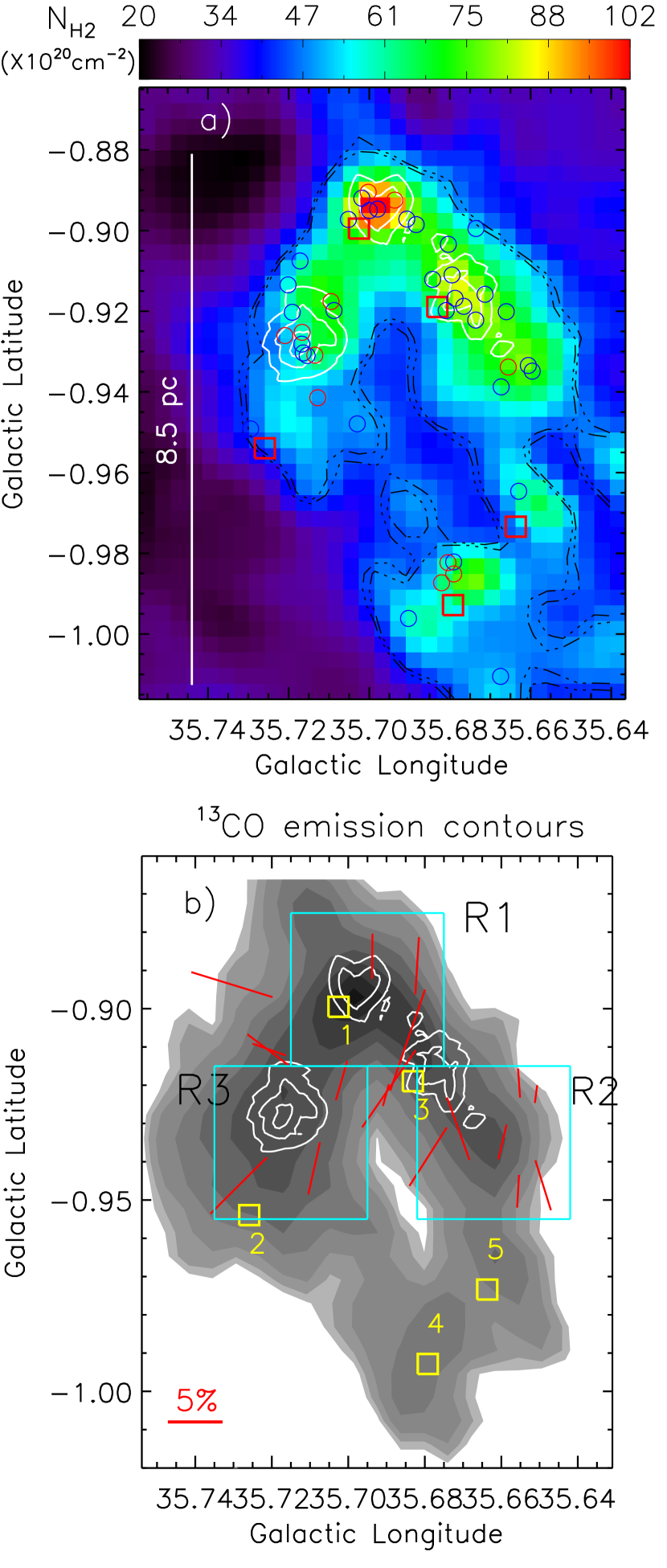
To probe the magnetic field morphology using starlight polarimetry, it is important to examine the relative polarization position angle orientations of the background stars with respect to the molecular cloud. In Section 2, we mentioned about the selection conditions to obtain the sources with reliable polarimetric information. These selected sources were further exposed to a color condition of JH 1 to depict the background stars that can successfully trace the POS magnetic field direction. A total of 462 stars have been selected in our target region around the G35.6 site. Figure 7a shows the observed H-band polarization of background starlight overlaid on the integrated molecular map. In Figure 7a, the degree of polarization is depicted by the length of a vector, whereas the angle of a vector shows the polarization Galactic position angle. In Figure 7a, in EMC1, we have also highlighted four subregions (i.e. R1, R2, R3, and R4) by boxes and each box has a size of 2′.4 2′.4. These subregions are associated with the areas of high column density in the Herschel column density map (see also Figure 6b).
In Figure 7b, we show the Planck polarization vectors (in blue) from the dust emission at . The vectors are rotated by 90∘ to show the POS magnetic field direction. The degree of polarization from the dust emission observed in the POS also depends on the variations of magnetic field along the line-of-sight (LOS). This causes de-polarization effects in the measurement. Since we are studying only the magnetic field direction using the Planck data, we average all the polarization values across the region, resulting in equal values in the degree of polarization. This exercise leads to the same length for all the vectors, keeping their original position angles. The Planck data at 353 GHz have a beam size of 5′ with a pixel scale of 1′.5 (1.6 pc at a distance of 3.7 kpc). In order to compare the magnetic field direction from the 353 GHz dust emission polarimetry and the NIR polarimetry, we calculate the mean polarization of the GPIPS data by spatially averaging the values matching the same pixel scale of the Planck data. The GPIPS polarization data are gridded into maps with box regions of 1′.5 1′.5. All the Stokes and values within each box region are combined by variance-weighted mean with their corresponding errors. The mean stokes values for each region are then used to compute the Ricean corrected de-biased polarization percentages and position angles for each box region (e.g. Clemens et al., 2012b). The mean GPIPS polarization values are shown in red, along with the Planck polarization vectors (in blue) in Figure 7b.
In Figure 7b, the Planck and GPIPS polarization vectors are in agreement with their relative position angles. However, one can notice differences in the orientation of the Planck and GPIPS vectors toward the molecular condensations (or areas of high column density). The Planck data show higher SNR results toward the molecular condensations due to the strong dust emission, whereas the GPIPS data toward the molecular condensations have a few measurements with low SNR due to high extinction. In EMC1, the distribution of polarization vectors appears different toward the ring-like feature and the semi-ring-like structure, implying a change in the magnetic field morphology between the two features.
Figures 8a and 8b show a zoomed in view of the ring-like feature using the Herschel column density and integrated molecular maps, respectively. These maps are also overlaid with the GPIPS H-band polarization vectors (having , , and ) and the Herschel clumps. A total of 17 stars are detected toward the ring-like feature, tracing the POS magnetic field direction. Table 3 lists the 2MASS photometric magnitudes, degree of polarization, and polarization Galactic position angles of these 17 stars. The degree of polarization for the 17 sources varies between 2 to 6%, whereas the polarization Galactic position angles have a dispersion of around 25∘ (see Table 3). With the help of the molecular gas distribution and the polarization data, we can characterize the orientation of polarization position angles with respect to the semi-major axis of the molecular structure. Fitting an ellipse to the ring-like feature (see Figure 8b), we find that the angle of the major axis of the ellipse is about 10. The mean polarization angles in three subregions R1, R2, and R3 are computed to be about 175, 177, and 169, respectively, and are measured from North-up, counter-clockwise (see Figure 7a). The difference between the polarization angle and the ellipse major axis is about 15. This indicates that the POS magnetic field is nearly parallel to the major axis of the ring-like feature. In Figures 7a and 7b, the semi-ring-like feature is seen at the northern part of EMC1. Similarly, we fit a semi-ellipse to the semi-ring-like feature and obtain the angle of the major axis to be 150. The mean polarization angle in the subregion R4 linked with the semi-ring-like feature is about 55. The difference between the polarization angle and the major axis is about 95, indicating that the POS field orientation is perpendicular to the molecular structure associated with the subregion R4.
3.6.2 Magnetic field strength
The POS magnetic field strength can be computed using the observed polarimetric data, in combination with gas motions and density from the molecular line data, following the equation given in Chandrasekhar & Fermi (1953) (hereafter CF-method). The CF-method as modified by Ostriker et al. (2001) can be presented in the following manner:
| (11) |
where is the POS magnetic field strength (in G), is the polarization position angle (P.A.) dispersion (in radians), is the gas volume mass density (in g cm-3), and is the 13CO gas velocity dispersion (in cm s-1). Ostriker et al. (2001) also suggested that the modified CF-method is applicable only when P.A. dispersion values are within (i.e. ).
To measure the magnetic field strength in the denser subregions within EMC1, we have carefully chosen four subregions (R1-R4) and the size of each subregion is 2′.4 2′.4 (as highlighted by boxes in Figure 7a). These subregions are centered around the Herschel clumps/molecular condensations. They are small enough to probe the magnetic field strength to few parsec scales and also big enough to have sufficient high quality polarization stars to measure the P.A. dispersion accurately.
The P.A. dispersion () is calculated by finding the standard deviation of the P.A. values within each box region. Since the P.A. values have an ambiguity of 0∘ and 180∘, dealiasing is necessary. This is done by finding the minimum of the dispersion values obtained for different sets of biased P.A. values. The biasing is carried out by stepping the P.A. values through increments of 1∘ between 0∘ and 180∘ producing different sets of biased P.A. values. The standard deviation for each set is computed and the minimum of the different standard deviation values is chosen as the final dispersion value. Note that typically, five polarization vectors are needed to obtain an accurate value of the P.A. dispersion. In the present case, we have only three polarization vectors in the subregion R3, where the derived P.A. dispersion is about 17. Considering this dispersion value, we can obtain a lower limit of the B-field in the subregion R3.
The gas velocity dispersion () is computed from the 13CO line profile for each pixel within the subregion. The line profile is fitted with a Gaussian to obtain the velocity dispersion as the width of the Gaussian. Multiple dispersion values within our selected box regions are then combined by median filtered mean to obtain the average dispersion value to be used in the CF-method for each region. A mean spectrum toward each subregion is presented in Figure 9.
The Herschel column density map is used to determine the volume densities for the four subregions in EMC1. Based on the ring-like structure assuming a face-on view, we assume a spherically oblate morphology for the cloud structure. Using this morphology we estimate the cloud thickness to be 4 pc. Based on the cloud thickness and the column densities, we calculate the volume number density of the region. The volume densities were gridded as a map having a spatial resolution of 14. All the volume densities within our each selected box region are then averaged to obtain the mean volume density. This is then converted into volume mass density by taking into account the molecular hydrogen’s weight (2 1.00794 1.67 10-24 gm) and a factor of 1.36 to account for helium and heavier elements. With the application of the CF-method, the POS magnetic field strength in each subregion has been estimated (see Table 4). Using the values of , we have also estimated magnetic pressure, (= ; dynes cm-2), equal to 1.8 10-11, 4.8 10-12, 4.8 10-12, and 1.6 10-11 dynes cm-2 for the subregions R1, R2, R3, and R4, respectively. The average magnetic field strength for all the subregions is computed to be about and the corresponding magnetic pressure is estimated to be 8.9 10-12 dynes cm-2.
We have also obtained the total field strength by assuming equipartition of magnetic, gravitational, and kinetic energy using a relation given in Lada et al. (2004) (i.e. = VNT (3/2ln2)1/2; where VNT is the nonthermal component of the observed line width). The non-thermal velocity dispersion is given by:
| (12) |
where (=(8 ln 2 2)1/2) is the measured full width at half maximum (FWHM) of the observed 13CO spectra, (= ) is the thermal broadening for 13CO at T, and is the mass of the hydrogen atom. In the Herschel temperature map, the ring-like feature is depicted in a temperature range of about 18–20 K. Using the values of and (at T = 20 K; see Section 3.5), we derive VNT, and then the values of BEP are estimated to be 9.5, 8.8, 8.8, and 6.3 for subregions R1, R2, R3, and R4, respectively.
The values of BEP are slightly lower than that of . In general, an equipartition stage indicates that all the forces are equal. However, based on the observations, we find that the magnetic field may have played a dominant role in the cloud formation and its evolution.
3.6.3 Mass to Flux Ratio
The knowledge of the magnetic field strength and “mass-to-flux (M/)” ratio can enable to infer the magnetically subcritical and supercritical clouds/cores. These parameters can also allow to observationally assess the molecular clouds/cores stability and can help to understand the ongoing physical process in the cloud. However, the observational measurement of M/ of a cloud core is a difficult experiment (e.g. Clemens et al., 2016, and references therein).
The normalized mass-to-flux ratio () can be calculated from magnetic field strength as follows (Crutcher et al., 2004):
| (13) |
where is the column density (in cm-2) and is the 3-Dimensional magnetic field strength (in G). Note that in equation 13, refers to the 3D magnetic field strength while our estimates are the POS magnetic field strength. Assuming that the LOS magnetic field is zero then one can replace with . However, in this case, will represent a lower limit to the total field strength. Hence, the mass-to-flux ratios of the four subregions are upper limit values. To obtain the corrected normalized mass-to-flux ratio, Planck Collaboration XXXV (2016c) report a correction factor of 1/3 and 3/4 for cloud geometries having magnetic field perpendicular and parallel to their major axis, respectively. In the ring-like feature, the magnetic field is parallel to its major axis. Hence, we applied a correction factor of 3/4 to the mass-to-flux ratio calculation for subregions R1, R2, and R3. In the semi-ring-like feature, the magnetic field is perpendicular to its major axis, favouring a correction factor of 1/3 for computing the mass-to-flux ratio in the subregion R4.
Using the POS magnetic field strength and the Herschel column density map, we have calculated the normalized mass-to-flux ratio for four subregions in EMC1. Three subregions (R1-R3) in EMC1 have mass-to-flux ratio greater than 1, implying the cloud is supercritical, while the subregion R4 is subcritical due to mass-to-flux ratio less than 1. In the subcritical region, the magnetic field dominates over gravity. On the other hand, in the supercritical region, the magnetic field cannot prevent gravitational collapse and hence the cloud can evolve and fragment into denser cores. Table 4 lists the magnetic properties for all the four subregions (R1-R4) in EMC1.
3.7. Young stellar population in MCG35.6
3.7.1 Selection of YSOs
In this section, to identify embedded YSOs within the MCG35.6, we have utilized the photometric data at 1–24 m
extracted from various infrared photometric surveys (e.g., MIPSGAL, GLIMPSE, UKIDSS-GPS, and 2MASS).
These data sets enable us to infer infrared excess sources.
The infrared excess emission around YSOs is explained by the presence of an envelope and/or circumstellar disk.
Previously, Paron et al. (2011) also presented 36 YSOs identified using the 2MASS and GLIMPSE 3.6–8.0 m
photometric data sets, which were restricted only within the EMC1 (see Figure 6 and Table 2 in Paron et al., 2011).
In the present work, we have utilized the UKIDSS-GPS NIR data, in combination with the GLIMPSE 3.6–8.0 m and
MIPSGAL 24 m data for depicting infrared excess sources.
Note that the UKIDSS-GPS NIR survey is three magnitudes deeper than 2MASS.
Hence, our present analysis will allow us to trace more deeply embedded and faint YSOs compared to previously published work.
A brief description of the selection of YSOs is as follows.
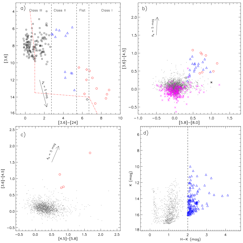
1. Using the Spitzer 3.6 and 24 m photometric data, Guieu et al. (2010) used a color-magnitude
plot ([3.6][24]/[3.6]) to identify the different stages of YSOs (see also Rebull et al., 2011; Dewangan et al., 2015; Dewangan, 2017b).
The color-magnitude plot is also utilized to distinguish the boundary of possible contaminants
(i.e. galaxies and disk-less stars) against YSOs (see Figure 10 in Rebull et al., 2011).
We have adopted this scheme in this work and the color-magnitude plot is shown in Figure 10a.
Following the conditions adopted in Guieu et al. (2010) and Rebull et al. (2011), the boundaries of different stages of
YSOs and possible contaminants are highlighted in Figure 10a.
In Figure 10a, a total of 164 sources are shown in the color-magnitude space.
We identify 24 YSOs (7 Class I; 4 Flat-spectrum; 13 Class II) and 139 Class III sources.
Additionally, one Flat-spectrum source is found in the boundary of possible contaminants and is excluded from our selected YSOs.
In Figure 10a, the selected Class I, Flat-spectrum, and Class II YSOs are highlighted
by red circles, red diamonds, and blue triangles, respectively.
2. Using the Spitzer 3.6, 4.5, 5.8, and 8.0 m photometric data, Gutermuth et al. (2009) provided
various schemes to identify the YSOs and also
various possible contaminants (e.g. broad-line active galactic nuclei (AGNs), PAH-emitting galaxies, shocked emission
blobs/knots, and PAH-emission-contaminated apertures). Furthermore, the selected YSOs can be further
classified into different evolutionary stages based on their
slopes of the SED () estimated from 3.6 to 8.0 m
(i.e., Class I (), Class II (),
and Class III ()) (e.g., Lada et al., 2006). More details about the YSO classifications
based on the Spitzer 3.6–8.0 m bands can be found in Dewangan and Anandarao (2011). Following the conditions
given in Gutermuth et al. (2009) and Lada et al. (2006), we have also identified YSOs and various possible contaminants
in our selected region around the G35.6 site. The Spitzer-GLIMPSE color-color plot ([3.6][4.5] vs [5.8][8.0]) is shown in Figure 10b.
Using the Spitzer 3.6–8.0 m photometric data, we find 28 YSOs (8 Class I; 20 Class II), 1 Class III, and 222 contaminants.
In Figure 10b, the selected Class I and Class II YSOs are highlighted by red circles and blue triangles, respectively.
3. Taking into account the sources having detections in the first three Spitzer-GLIMPSE bands (except 8.0 m band), Hartmann et al. (2005) and Getman et al. (2007) use a color-color plot ([4.5][5.8] vs [3.6][4.5]) to identify the YSOs. They use color conditions, [4.5][5.8] 0.7
and [3.6][4.5] 0.7, to select protostars.
Using the first three Spitzer-GLIMPSE bands, we obtain 4 protostars in our selected region (see Figure 10c).
4. In this YSO classification scheme, the NIR color-magnitude space (HK/K) is utilized to identify additional YSOs.
We use a color HK value (i.e. 2.0) that divides the HK excess sources from the rest of the population.
This color condition is adopted based on the color-magnitude plot of sources from the nearby control field
(size of the selected region 121 87; centered at: = 35.484; = 0.67).
Using the color HK cut-off condition, we find 142 embedded YSOs in the region probed in this work (see Figure 10d).
All together, the analysis of the photometric data at 1–24 m gives a total of 198 YSOs in our selected region around the G35.6 site. In Figure 11a, these selected YSOs are overlaid on the integrated molecular map, helping to infer the YSOs belonging to the MCG35.6. We find 59 YSOs in the direction of EMC1, while 15 YSOs are identified toward EMC2. In the EMC1, we have found a larger number of YSOs compared to the previously reported work of Paron et al. (2011) (see Table 2 in their paper). Table 5 lists the NIR and Spitzer photometric magnitudes of the 59 YSOs seen toward EMC1, which are identified using the color-magnitude and color-color plots. The table also gives the information about the classification stages of YSOs. In EMC1, we find noticeable YSOs toward one of the edges of the semi-ring-like morphology. Furthermore, several YSOs are also distributed toward the ring-like feature in EMC1.
3.7.2 Young stellar clusters in MCG35.6
In this section, we probe the individual groups or clusters of YSOs based on their spatial distribution and the statistical surface density utility. The clusters of YSOs within the MCG35.6 are still unknown. In star-forming regions, the surface density map of selected YSOs is often generated using the nearest-neighbour (NN) technique (see Gutermuth et al., 2009; Bressert et al., 2010; Dewangan et al., 2015, 2017a; Dewangan, 2017b, for more details). The surface density map can be obtained by dividing the selected field using a regular grid and extracting the surface density of YSOs at each grid point. The surface number density at the kth grid point is given by (e.g. Casertano & Hut, 1985), where denotes the surface area defined by the radial distance to the = 6 NN. Adopting this procedure, the surface density map of all the selected 198 YSOs has been constructed using a 5 grid and 6 NN at a distance of 3.7 kpc. In Figure 11b, we show the surface density contours of YSOs overlaid on the Herschel column density map. The YSOs density contours are drawn at 3, 5, and 10 YSOs/pc2, increasing from the outer to the inner regions. The positions of Herschel clumps are also shown in Figure 11b. The YSO clusters are seen toward Herschel clumps (i.e., nos. 1, 2, 3, and 8). Additionally, noticeable YSOs are also found toward the Herschel clumps nos. 4 and 5 without any clustering. Earlier in Section 3.5, the five clumps (i.e., nos. 1, 2, 3, 4, and 5) have been seen at the edges of the ring-like feature (see a solid yellow box in Figure 6b). Figures 12a and 12b also show the spatial distribution of YSOs toward the ring-like feature, depicting the ongoing star formation activities on the edges of the ring-like feature.
Star formation activity is also observed toward the clump no. 8 in EMC2. Furthermore, we find surface density contours of YSOs away from the 13CO emission, implying that these clusters are not directly associated with MCG35.6.
4. Discussion
4.1. H ii regions in EMC1
A careful multi-wavelength data analysis reveals two distinct structures (i.e. semi-ring-like and ring-like structures) in the EMC1. The semi-ring-like structure is associated with the radio source crs1, and is possibly produced by the ionizing feedback of a B0.5V or B0V type star (see Section 3.4). On the other hand, if the ring-like feature was produced by feedback of a massive star then, there should be ionized gas inside the structure produced by a massive star located within the ring-like feature. Since there are no evidences of the existence of this star or of ionized gas (at the sensitivity of the observed NVSS radio map; 1 0.45 mJy beam-1), then the ring-like feature is unlikely to be originated by the feedback of a massive star. However, with the sensitivity limit of the NVSS data, one cannot completely rule out the presence of a massive B2-B3 star, or even a cluster of B3 stars, producing the cavity in the ring-like structure. Furthermore, the north-western side of the ring-like feature appears to be influenced by the feedback of the massive star linked with the radio source crs2 (see Section 3.4).
The photometric analysis of point-like sources reveals a population of YSOs toward the edges of the semi-ring-like and ring-like structures (see Section 3.7.1). Hence, star formation activities are traced within EMC1 (see Figure 11a and also Section 3.7). The young stellar populations can be originated spontaneously in a given molecular cloud, or the process of collapse and star formation can also be influenced by some external agents such as the expansion of H ii regions (e.g., Elmegreen, 1998). Hence, a triggered star formation scenario (via an expanding H ii region) appears applicable in the G35.6 site. The dynamical or expansion ages of the H ii regions are estimated to be 0.35–0.5 Myr (for n0 = 103 cm-3; see Section 3.3, see also Paron et al., 2011), which can be treated as the indicative values or the lower limits to the actual ages. Evans et al. (2009) estimated the average lifetimes of Class I and Class II YSOs to be 0.44 Myr and 1–3 Myr, respectively. Based on the comparison of these typical ages of YSOs and the dynamical ages of the H ii regions, we cannot completely rule out the formation of Class I YSOs through the expansion of the H ii regions in EMC1. However, the majority of selected young populations in EMC1 are Class II YSOs (see Table 5; 51 Class II candidates out of 59 YSOs). Hence, the clusters of YSOs are unlikely to be originated by the expansion of the H ii regions linked with crs1 and crs2.
4.2. Formation and evolution of features in EMC1
The embedded ring-like feature in EMC1 is the most prominent structure evident in the 13CO integrated intensity and Herschel column density maps (see Figures 8a and 8b). The ring-like feature with a face-on view has a central region/cavity devoid of radio continuum emission. The structure in the sky of the ring-like feature can be a spherically oblate cloud.
From a theoretical point of view, the formation of a ring-like feature can be explained by the ambipolar diffusion, when the cloud was magnetically subcritical. Conditions with low density perturbations and thermal pressure allow the cloud to condense along the field lines to form the oblate morphologies. When the cloud axis is non-axisymmetric, the magnetically mediated cloud condensation forms a ring-like feature with dense supercritical cores (Fiedler & Mouschovias, 1993). Li & Nakamura (2002) also carried out numerical simulations to examine the evolution of subcritical clouds by considering the non-axisymmetric case under thin-disk approximation. They reported that a magnetically subcritical cloud fragments into multiple magnetically supercritical cores, when the density perturbations are very large. Eventually, these supercritical cores lead to the birth of a new generation of stars in small clusters through gravitationally dominated ambipolar diffusion.
A detailed analysis of the GPIPS and Planck polarimetric data indicates that the magnetic field is parallel to the major axis of the ring-like feature. Our analysis on magnetic field properties further suggests that three subregions (i.e. R1, R2, and R3) in the ring-like feature are magnetically supercritical and each subregion hosts at least one Herschel clump (see Section 3.6.3). We find at least five clumps (i.e., nos. 1, 2, 3, 4, and 5; see Figure 8a) at the edges of this ring-like feature which seem to be spatially distributed in an almost regularly spaced manner, indicating the fragmentation of the ring-like feature. A population of YSOs is found toward all the five clumps including three magnetically supercritical clumps (see Section 3.7.2 and Figures 12a and 12b). One can note that the subregion R2 is seen in the direction of the north-western side of the ring-like feature, where the impact of the massive star linked with the radio source crs2 cannot be ignored (see Section 3.4). However, in the subregion R2, the origin of Class II YSOs through the expansion of the H ii region is unlikely (see Section 4.1).
Furthermore, we have also investigated the magnetic field properties in the subregion R4 located at one of the edges of the semi-ring-like morphology (see Section 3.6). The field orientation obtained from the GPIPS H-band polarization appears perpendicular to the major axis of the molecular structure linked with the subregion R4 (see Figure 7a). As mentioned earlier, the subregion R4 is magnetically subcritical. Additionally, there is no signature of star formation activity in this particular subregion (see Section 3.7). This implies that the magnetic field might be dynamically important in the formation and evolution of the semi-ring like feature (e.g. Mouschovias, 1978).
Our observational results are in agreement with the outcomes of the numerical simulations concerning the evolution of the magnetically subcritical cloud (see Li & Nakamura, 2002), which fragments into multiple magnetically supercritical clumps and further leads to birth of multiple stars/systems or clusters.
5. Summary and Conclusions
In this paper, to probe the physical processes and star formation activity,
we have carried out an extensive study of the G35.6 site using multi-wavelength data.
Our analysis has been focused on the distribution of the ionized gas, molecular gas, cold dust, magnetic field, and embedded young populations. The important findings of this work are:
The molecular cloud associated with the G35.6 site (i.e. MCG35.6) is depicted in the velocity range 53–62 km s-1. In our selected region around the G35.6 site,
two extended molecular condensations (i.e., EMC1 and EMC2) are observed.
The molecular data trace two molecular components in the direction of the G35.6 site.
A molecular component associated with EMC1 is depicted in the velocity range 53–59 km s-1,
while the other molecular component associated with EMC2 is observed at 59–62 km s-1.
A careful analysis of the molecular line data shows that these two molecular components are clearly separated in both
space and velocity, and seem to be unrelated molecular clouds.
In EMC1, the multi-wavelength images reveal the existence of a semi-ring-like feature (associated with the ionized gas emission) and
an embedded face-on ring-like feature devoid of radio continuum emission in its center.
The detection/non-detection of the ionized gas emission in the G35.6 site is obtained from the NVSS radio continuum map at 1.4 GHz, which has the sensitivity limit of 0.45 mJy beam-1.
Two compact radio continuum sources (i.e., crs1 and crs2) are associated with EMC1.
The NVSS 1.4 GHz continuum data analysis reveals that each H ii region is excited
by a B0.5V–B0V type star and has a dynamical age of 0.35–0.5 Myr.
The Herschel temperature map reveals the heating from the two compact radio continuum sources with temperatures 22–27 K,
while the ring-like feature has a temperature range of about 18–20 K.
In the Herschel column density map, at least five massive Herschel clumps ( 740–1420 M⊙)
seem to be spatially distributed in an almost regularly spaced manner along the ring-like feature.
The analysis of photometric data at 1–24 m reveals a total of 198 YSOs. Most of these YSOs are spatially distributed
toward the Herschel clumps in EMC1.
Star formation activities have been found toward the clumps seen at the edges of the ring-like feature in EMC1.
The Planck and GPIPS polarimetric data trace the POS magnetic field parallel to the major axis of the ring-like feature.
Using the GPIPS H-band polarimetric data, three magnetically supercritical subregions containing the Herschel clumps
are observed in the ring-like feature.
Considering our observational findings, the semi-ring-like feature is resultant of the ionizing feedback of a massive star linked with the radio source crs1. On the other hand, the existence of a ring-like feature cannot be explained by the impact of massive star(s). Our observational analysis favors the idea that the ring-like feature may have formed from a magnetically dominated cloud. The results derived using the molecular emission, cold dust emission, and magnetic field properties reveal that the ring-like feature contains multiple supercritical clumps that can potentially fragment into dense cores, eventually leading to the birth of multiple stars/systems or clusters. These findings can be linked to the formation and evolution of the cloud via the magnetic field mediated mechanism as suggested by Li & Nakamura (2002).

.
| Survey | Wavelength(s) | Resolution () | Reference |
|---|---|---|---|
| Two Micron All Sky Survey (2MASS) | 1.25–2.2 m | 2.5 | Skrutskie et al. (2006) |
| Galactic Plane Infrared Polarization Survey (GPIPS) | 1.6 m | 1.5 | Clemens et al. (2012a) |
| UKIRT NIR Galactic Plane Survey (GPS) | 1.25–2.2 m | 0.8 | Lawrence et al. (2007) |
| Spitzer Galactic Legacy Infrared Mid-Plane Survey Extraordinaire (GLIMPSE) | 3.6, 4.5, 5.8, 8.0 m | 2, 2, 2, 2 | Benjamin et al. (2003) |
| Wide Field Infrared Survey Explorer (WISE) | 3.4, 4.6, 12, 22 m | 6, 6.5, 6.5, 12 | Wright et al. (2010) |
| Spitzer MIPS Inner Galactic Plane Survey (MIPSGAL) | 24 m | 6 | Carey et al. (2005) |
| Herschel Infrared Galactic Plane Survey (Hi-GAL) | 70, 160, 250, 350, 500 m | 5.8, 12, 18, 25, 37 | Molinari et al. (2010) |
| Planck polarization data | 850 m | 294 | Planck Collaboration IX (2014) |
| Galactic Ring Survey (GRS) | 2.7 mm; 13CO (J = 1–0) | 45 | Jackson et al. (2006) |
| Coordinated Radio and Infrared Survey for High-Mass Star Formation (CORNISH) | 6 cm | 1.5 | Hoare et al. (2012) |
| NRAO VLA Sky Survey (NVSS) | 21 cm | 45 | Condon et al. (1998) |
| ID | l | b | Rc | peak N(H2) | AV | |
|---|---|---|---|---|---|---|
| (degree) | (degree) | (pc) | () | (1021 cm-2) | (mag) | |
| 1† | 35.702 | -0.899 | 1.7 | 1150 | 10 | 11 |
| 2† | 35.726 | -0.954 | 1.5 | 740 | 5.4 | 6 |
| 3† | 35.683 | -0.919 | 1.9 | 1420 | 8.5 | 9 |
| 4† | 35.679 | -0.993 | 1.9 | 1275 | 7.7 | 8 |
| 5† | 35.664 | -0.973 | 1.7 | 950 | 6.6 | 7 |
| 6 | 35.854 | -0.946 | 1.5 | 715 | 5.9 | 6 |
| 7 | 35.881 | -0.927 | 1.2 | 450 | 5.6 | 6 |
| 8 | 35.831 | -0.864 | 3.2 | 3390 | 9.1 | 10 |
| 9 | 35.897 | -0.911 | 0.8 | 175 | 4.2 | 5 |
| l | b | J-band | H-band | K-band | P | sP | GPA | sPA |
|---|---|---|---|---|---|---|---|---|
| (deg) | (deg) | (mag) | (mag) | (mag) | (%) | (%) | (deg) | (deg) |
| 35.682 | -0.888 | 15.54 | 11.97 | 10.22 | 5.23 | 1.77 | 176.41 | 9.69 |
| 35.655 | -0.919 | 12.01 | 9.61 | 8.47 | 2.67 | 0.33 | 3.94 | 3.57 |
| 35.650 | -0.922 | 11.71 | 10.50 | 10.02 | 1.62 | 0.28 | 172.62 | 5.07 |
| 35.684 | -0.908 | 16.63 | 12.98 | 11.27 | 9.76 | 2.09 | 160.99 | 6.14 |
| 35.659 | -0.934 | 16.84 | 12.82 | 10.53 | 3.24 | 1.31 | 166.80 | 11.6 |
| 35.689 | -0.920 | 15.61 | 12.86 | 11.59 | 8.56 | 2.46 | 145.21 | 8.24 |
| 35.671 | -0.931 | 15.37 | 12.67 | 11.43 | 6.07 | 1.72 | 19.81 | 8.13 |
| 35.690 | -0.922 | 11.36 | 8.81 | 7.45 | 2.04 | 0.57 | 164.50 | 8.05 |
| 35.649 | -0.946 | 15.81 | 12.03 | 10.31 | 4.77 | 1.06 | 17.35 | 6.37 |
| 35.655 | -0.947 | 12.56 | 10.12 | 9.00 | 2.98 | 0.23 | 176.77 | 2.23 |
| 35.679 | -0.938 | 13.70 | 12.32 | 11.55 | 6.33 | 1.45 | 147.44 | 6.59 |
| 35.693 | -0.886 | 15.55 | 11.76 | 9.79 | 4.12 | 1.58 | 179.38 | 11.01 |
| 35.730 | -0.893 | 14.50 | 12.78 | 11.92 | 7.77 | 2.61 | 72.90 | 9.63 |
| 35.701 | -0.918 | 13.60 | 11.85 | 11.15 | 3.75 | 1.49 | 163.90 | 11.43 |
| 35.720 | -0.910 | 14.65 | 11.94 | 10.66 | 3.21 | 1.45 | 70.58 | 12.93 |
| 35.708 | -0.941 | 14.00 | 11.42 | 10.23 | 4.88 | 1.17 | 167.34 | 6.90 |
| 35.728 | -0.946 | 15.20 | 12.57 | 11.35 | 7.27 | 3.28 | 134.94 | 12.91 |
| subregion | l | b | ||||||
|---|---|---|---|---|---|---|---|---|
| (degree) | (degree) | (degree) | (km s-1) | (cm-3) | (G) | ( 10-11 dynes cm-2) | ||
| 1 | 35.695 | -0.895 | 9.9 | 0.79 | 469 | 21.5 | 1.8 | 1.5 |
| 2 | 35.665 | -0.935 | 18.1 | 0.73 | 465 | 11.0 | 0.48 | 3.0 |
| 3 | 35.715 | -0.935 | 17.8 | 0.78 | 407 | 11.0 | 0.48 | 2.6 |
| 4 | 35.725 | -0.845 | 7.0 | 0.68 | 275 | 20.0 | 1.6 | 0.4 |
| ID | YSO | l | b | J | H | K | 3.6 m | 4.5 m | 5.8 m | 8.0 m | 24 m |
|---|---|---|---|---|---|---|---|---|---|---|---|
| (stage,scheme) | (degree) | (degree) | (mag) | (mag) | (mag) | (mag) | (mag) | (mag) | (mag) | (mag) | |
| 1 | I,sh1 | 35.696 | -0.841 | — | — | — | 13.18 | 11.30 | 9.67 | 8.56 | 4.36 |
| 2 | I,sh1 | 35.700 | -0.891 | — | — | 13.45 | 10.95 | 9.76 | 8.86 | 8.32 | 4.18 |
| 3 | II,sh1 | 35.713 | -0.931 | — | — | 13.52 | 11.18 | 10.30 | 9.74 | 9.23 | 6.37 |
| 4 | I,sh2 | 35.709 | -0.918 | — | — | — | 13.58 | 13.15 | 11.98 | 11.30 | — |
| 5 | I,sh2 | 35.680 | -0.982 | — | 11.46 | 9.54 | 7.42 | 6.71 | 5.99 | 4.83 | — |
| 6 | I,sh2 | 35.679 | -0.985 | — | — | 14.58 | 11.91 | 10.94 | 10.26 | 9.52 | — |
| 7 | II,sh2 | 35.681 | -0.829 | 15.83 | 13.62 | 12.49 | 11.28 | 10.69 | 10.05 | 9.18 | — |
| 8 | II,sh2 | 35.684 | -0.841 | — | — | — | 11.55 | 11.05 | 10.49 | 9.96 | — |
| 9 | II,sh2 | 35.685 | -0.836 | — | 15.05 | 13.74 | 12.10 | 11.56 | 11.06 | 10.51 | — |
| 10 | II,sh2 | 35.703 | -0.823 | 16.51 | 14.15 | 12.97 | 12.08 | 11.60 | 11.26 | 10.29 | — |
| 11 | II,sh2 | 35.682 | -0.987 | — | 14.68 | 13.58 | 11.71 | 11.03 | 10.65 | 10.11 | — |
| 12 | II,sh2 | 35.717 | -0.925 | 15.78 | 13.61 | 12.11 | 10.11 | 9.57 | 8.99 | 8.21 | — |
| 13 | II,sh2 | 35.713 | -0.941 | 15.71 | 14.11 | 13.15 | 11.80 | 11.20 | 10.72 | 10.14 | — |
| 14 | II,sh2 | 35.638 | -0.834 | — | — | — | 13.36 | 12.53 | 12.15 | 11.33 | — |
| 15 | I,sh3 | 35.666 | -0.934 | — | — | — | 14.95 | 13.17 | 11.49 | 11.34 | — |
| 16 | I,sh3 | 35.694 | -0.892 | — | — | 14.27 | 12.43 | 11.68 | 10.82 | — | — |
| 17 | I,sh3 | 35.721 | -0.926 | — | 14.99 | 13.38 | 10.98 | 9.86 | 9.11 | 8.36 | — |
| 18 | II,sh4 | 35.661 | -0.933 | 17.91 | 14.13 | 12.07 | 10.73 | 10.59 | 10.27 | 10.45 | — |
| 19 | II,sh4 | 35.671 | -0.916 | 18.62 | 14.78 | 12.65 | 11.33 | 11.18 | 10.92 | — | — |
| 20 | II,sh4 | 35.703 | -0.948 | 20.39 | 17.77 | 15.56 | 14.38 | 14.13 | — | — | — |
| 21 | II,sh4 | 35.677 | -0.919 | — | 17.93 | 14.89 | 12.77 | 12.51 | — | — | — |
| 22 | II,sh4 | 35.639 | -0.811 | 18.51 | 14.60 | 12.38 | 10.91 | 10.74 | 10.45 | 10.47 | — |
| 23 | II,sh4 | 35.638 | -0.961 | — | 16.99 | 14.96 | 14.03 | 13.40 | — | — | — |
| 24 | II,sh4 | 35.633 | -0.960 | — | 15.24 | 12.34 | 10.82 | 10.52 | 10.08 | 10.12 | — |
| 25 | II,sh4 | 35.666 | -0.920 | — | 16.39 | 14.34 | 13.04 | 12.91 | — | — | — |
| 26 | II,sh4 | 35.684 | -0.912 | — | 17.74 | 15.45 | 13.43 | 12.91 | 12.22 | — | — |
| 27 | II,sh4 | 35.667 | -0.939 | — | 16.23 | 14.11 | 12.69 | 12.62 | — | — | — |
| 28 | II,sh4 | 35.679 | -0.917 | — | 17.96 | 15.95 | 13.45 | 13.36 | — | — | — |
| 29 | II,sh4 | 35.679 | -0.911 | — | 16.92 | 13.53 | 11.18 | 10.87 | 10.41 | 11.05 | — |
| 30 | II,sh4 | 35.681 | -0.920 | — | 17.39 | 15.26 | 13.62 | 13.26 | — | — | — |
| 31 | II,sh4 | 35.680 | -0.903 | — | 14.68 | 11.43 | 9.34 | 9.07 | 8.55 | 8.59 | — |
| 32 | II,sh4 | 35.663 | -0.965 | — | 17.71 | 15.20 | 13.76 | 13.62 | — | — | — |
| 33 | II,sh4 | 35.674 | -0.922 | — | 17.06 | 14.57 | 12.99 | 12.67 | 11.66 | — | — |
| 34 | II,sh4 | 35.674 | -0.900 | — | 18.05 | 16.00 | 14.46 | 14.03 | — | — | — |
| 35 | II,sh4 | 35.720 | -0.913 | — | 17.32 | 15.16 | 13.85 | 13.53 | — | — | — |
| 36 | II,sh4 | 35.700 | -0.895 | — | 18.02 | 16.02 | — | — | — | — | — |
| 37 | II,sh4 | 35.688 | -0.899 | — | 17.99 | 15.86 | 14.37 | 13.99 | — | — | — |
| 38 | II,sh4 | 35.636 | -0.804 | — | 15.40 | 12.78 | 11.13 | 10.81 | 10.42 | 10.30 | — |
| 39 | II,sh4 | 35.690 | -0.996 | — | 16.98 | 14.85 | — | — | — | — | — |
| 40 | II,sh4 | 35.667 | -1.011 | — | 17.32 | 15.08 | 13.69 | 13.53 | — | — | — |
| 41 | II,sh4 | 35.761 | -0.834 | 17.80 | 16.89 | 14.78 | — | — | — | — | — |
| 42 | II,sh4 | 35.677 | -0.843 | 19.74 | 16.46 | 14.34 | 12.22 | 11.53 | 10.91 | — | — |
| 43 | II,sh4 | 35.717 | -0.908 | 17.33 | 13.40 | 11.30 | 9.97 | 9.87 | 9.40 | 9.29 | — |
| 44 | II,sh4 | 35.705 | -0.897 | 19.30 | 14.60 | 12.29 | 10.82 | 10.70 | 10.22 | 10.19 | — |
| 45 | II,sh4 | 35.684 | -0.855 | 18.89 | 14.85 | 12.38 | 10.91 | 10.58 | 10.25 | 10.49 | — |
| 46 | II,sh4 | 35.717 | -0.928 | 19.24 | 15.67 | 13.66 | 12.52 | 12.12 | 11.78 | — | — |
| 47 | II,sh4 | 35.715 | -0.931 | 19.48 | 15.06 | 12.94 | 11.61 | 11.33 | 10.96 | 10.83 | — |
| 48 | II,sh4 | 35.719 | -0.920 | — | 17.89 | 15.56 | 14.06 | 13.85 | — | — | — |
| 49 | II,sh4 | 35.677 | -0.840 | — | 17.85 | 15.68 | 13.66 | 13.28 | — | — | — |
| 50 | II,sh4 | 35.702 | -0.892 | — | 17.68 | 15.54 | 14.16 | 13.93 | — | — | — |
| 51 | II,sh4 | 35.698 | -0.895 | — | 17.97 | 15.85 | — | — | — | — | — |
| 52 | II,sh4 | 35.709 | -0.920 | — | 17.35 | 14.87 | 13.48 | 12.85 | — | — | — |
| 53 | II,sh4 | 35.691 | -0.897 | — | 17.87 | 15.30 | 13.65 | 13.12 | — | — | — |
| 54 | II,sh4 | 35.638 | -0.808 | — | 17.60 | 14.84 | 12.94 | 12.42 | 12.11 | — | — |
| 55 | II,sh4 | 35.693 | -0.827 | — | 17.83 | 15.80 | 13.35 | 13.37 | — | — | — |
| 56 | II,sh4 | 35.729 | -0.949 | — | 17.02 | 14.81 | 13.43 | 13.19 | — | — | — |
| 57 | II,sh4 | 35.716 | -0.930 | — | 16.99 | 14.56 | 13.01 | 12.65 | — | — | — |
| 58 | II,sh4 | 35.679 | -0.982 | 15.36 | 14.16 | 12.04 | 10.25 | 9.92 | 9.25 | 8.52 | — |
| 59 | II,sh4 | 35.660 | -0.935 | 16.84 | 12.82 | 10.54 | 8.69 | 8.50 | 8.01 | 7.90 | 6.04 |
References
- Anderson et al. (2009) Anderson, L. D., Bania, T. M., Jackson, J. M., et al. 2009, ApJS, 181, 255
- Andersson et al. (2015) Andersson, B. G., Lazarian, A., Vaillancourt, J. E. 2015, ARA&A, 53, 501
- Arce et al. (2011) Arce, H. G., Borkin, M. A., Goodman, A. A., Pineda, J. E.,& Beaumont, C. N. 2011, ApJ, 742, 105
- Beaumont & Williams (2010) Beaumont, C. N., & Williams, J. P. 2010, ApJ, 709, 791
- Benjamin et al. (2003) Benjamin, R. A.,Churchwell, E., Babler, B. L., et al. 2003, PASP, 115, 953
- Bisbas et al. (2009) Bisbas, T. G., Wünsch, R., Whitworth, A. P., & Hubber, D. A. 2009, A&A, 497, 649
- Bohlin et al. (1978) Bohlin, R. C., Savage, B. D., & Drake, J. F. 1978, ApJ, 224, 13233
- Bressert et al. (2010) Bressert, E., Bastian, N., Gutermuth, R., et al. 2010, MNRAS, 409, 54
- Bressert et al. (2012) Bressert, E., Ginsburg, A., Bally, J., et al. 2012, ApJ, 758, 28
- Carey et al. (2005) Carey, S. J., Noriega-Crespo, A., Price, S. D., et al. 2005, BAAS, 37, 1252
- Casertano & Hut (1985) Casertano, S., & Hut P. 1985, ApJ, 298, 80
- Chandrasekhar & Fermi (1953) Chandrasekhar, S., & Fermi, E. 1953, ApJ, 118, 113
- Chen et al. (2017) Chen, Z., Jiang, Z., Tamura, M., Kwon, J., & Roman-Lopes, A. 2017, ApJ, 838, 80
- Churchwell et al. (2006) Churchwell, E., Povich, M. S., Allen, D., et al. 2006, ApJ, 649, 759
- Churchwell et al. (2007) Churchwell, E., Watson, D. F., Povich, M. S., et al. 2007, ApJ, 670, 428
- Clemens et al. (2012a) Clemens, D. P., Pavel, M. D., & Cashman, L. R. 2012a, ApJS, 200, 21
- Clemens et al. (2012b) Clemens, D. P., Pinnick, A., Pavel, M. D. et. al 2012b, ApJS, 200, 19
- Clemens et al. (2016) Clemens, D. P., Tassis, K., & Goldsmith, P. F. 2016, ApJ, 833, 176
- Condon et al. (1998) Condon, J. J., Cotton, W. D., Greisen, E. W., et al. 1998, AJ, 115, 1693
- Crutcher et al. (2004) Crutcher, R. M., Nutter, D. J., Ward-Thompson, D., et al. 2004, ApJ, 600, 279
- Davis & Greenstein (1951) Davis, L., Jr., & Greenstein, J. L. 1951, ApJ, 114, 206
- de Graauw et al. (2010) de Graauw, T., Helmich, F. P., Phillips, T. G., et al. 2010, A&A, 518, L4
- Deharveng et al. (2010) Deharveng, L., Schuller, F., Anderson, L. D., et al. 2010, A&A, 523, 6
- Dewangan and Anandarao (2011) Dewangan, L. K., & Anandarao, B. G 2011, MNRAS, 414, 1526
- Dewangan et al. (2015) Dewangan, L. K., Luna, A., Ojha, D. K., et al. 2015, ApJ, 811, 79
- Dewangan et al. (2016) Dewangan, L. K., Ojha, D. K., Luna, A., et al. 2016, ApJ, 819, 66
- Dewangan et al. (2017a) Dewangan, L. K., Ojha, D. K., Zinchenko, I., Janardhan, P., & Luna, A. 2017a, ApJ, 834, 22
- Dewangan (2017b) Dewangan, L. K. 2017b, accepted in ApJ, arXiv:1702.00007
- Dolginov & Mitrofanov (1976) Dolginov, A. Z., & Mitrofanov, I. G. 1976, Ap&SS, 43, 291
- Dyson & Williams (1980) Dyson, J. E., & Williams, D. A. 1980, Physics of the Interstellar Medium (New York: Halsted Press)
- Elmegreen (1998) Elmegreen, B. G. 1998, in ASP Conf. Ser. 148, Origins, ed. C. E. Woodward, J. M. Shull, & H. A. Thronson, Jr. (San Francisco, CA: ASP), 150
- Evans et al. (2009) Evans, N. J., II, Dunham, M. M., Jørgensen, J. K., et al. 2009, ApJS, 181, 321
- Flaherty et al. (2007) Flaherty, K. M., Pipher, J. L., Megeath, S. T., et al. 2007, ApJ, 663, 1069
- Fiedler & Mouschovias (1993) Fiedler, R., & Mouschovias, T. 1993, ApJ, 415, 680
- Getman et al. (2007) Getman, K. V., Feigelson, E. D., Garmire,G., Broos, P., & Wang, J. 2007, ApJ, 654, 316
- Goicoechea et al. (2017) Goicoechea, J. R., Cuadrado, S., Pety, J., et al. 2017, A&A, 601L, 9
- Górski et al. (2005) Górski, K. M., Hivon, E., Banday, A. J., et al. 2005, ApJ, 622, 759
- Griffin et al. (2010) Griffin, M. J., Abergel, A., Abreu, A, et al. 2010, A&A, 518L, 3
- Guieu et al. (2010) Guieu, S., Rebull, L. M., Stauffer, J. R., et al. 2010, ApJ, 720, 46
- Gutermuth et al. (2009) Gutermuth, R. A., Megeath, S. T., Myers, P. C., et al. 2009, ApJS, 184, 18
- Gutermuth & Heyer (2015) Gutermuth, R. A., & Heyer,M. 2015, AJ, 149, 64
- Hamaker & Bregman (1996) Hamaker, J. P. & Bregman, J. D. 1996, A&AS, 117, 161
- Hartmann et al. (2001) Hartmann, L., Ballesteros-Paredes, J., & Bergin, E. A. 2001, ApJ, 562, 852
- Hartmann et al. (2005) Hartmann, L., Megeath, S. T., Allen, L., et al. 2005, ApJ, 629, 881
- Hildebrand (1983) Hildebrand, R. H. 1983, QJRAS, 24, 267
- Hoare et al. (2012) Hoare, M. G., Purcell, C. R., Churchwell, E. B., et al. 2012, PASP, 124, 939
- Hollenbach & Tielens (1997) Hollenbach, D. J. & Tielens, A. G. G. M. 1997, ARA&A, 35, 179
- Jackson et al. (2006) Jackson, J. M., Rathborne, J. M., Shah, R. Y., et al. 2006, ApJS, 163, 145
- Kauffmann et al. (2008) Kauffmann, J., Bertoldi, F., Bourke, T. L., Evans, II, N. J.,& Lee, C. W. 2008, ApJ, 487, 993
- Kendrew et al. (2012) Kendrew, S., Simpson, R., Bressert, E., et al. 2012, ApJ, 755, 71
- Kurtz (2005) Kurtz, S. 2005, IAUS, 227, 111
- Kwan (1997) Kwan, J. 1997, ApJ, 489, 284
- Lada et al. (2004) Lada, C. J., Huard, T. L., Crews, L. J., & Alves, J. F. 2004, ApJ, 610, 303
- Lada et al. (2006) Lada, C. J., Muench, A. A., Luhman, K. L., et al. 2006, AJ, 131, 1574
- Lazarian (2007) Lazarian, A. 2007, J. Quant. Spec. Radiat. Transf. 106, 225
- Lawrence et al. (2007) Lawrence, A., Warren, S. J., Almaini, O., et al. 2007, MNRAS, 379, 1599
- Li & Nakamura (2002) Li, Z. Y. & Nakamura, F. 2002, ApJ, 578, 256
- Lockman (1989) Lockman, F. J. 1989, ApJS, 71, 469
- Lucas et al. (2008) Lucas, P. W., Hoare, M. G., Longmore, A., et al. 2008, MNRAS, 391, 1281
- Mallick et al. (2015) Mallick, K. K., Ojha, D. K., Tamura, M., et al. 2015, MNRAS, 447, 2307
- Martins et al. (2005) Martins, F., Schaerer, D., & Hillier, D. J. 2005, A&A, 436, 1049
- Matsakis et al. (1976) Matsakis, D. N., Evans, N. J., II, Sato, T., & Zuckerman, B. 1976, AJ, 81, 172
- Molinari et al. (2010) Molinari, S., Swinyard, B., Bally, J., et al., 2010, A&A, 518, L100
- Mouschovias (1978) Mouschovias, T. C. 1978, in IAU Colloq. 52: Protostars and Planets, ed. T. Gehrels, 209–242
- Nakamura & Li (2002) Nakamura, F. & Li, Z. Y. 2002, ApJ, 566, 101
- Olnon (1975) Olnon, F. M. 1975, A&A, 39, 217
- Oskinova et al. (2011) Oskinova, L. M., Todt, H., Ignace, R., et al. 2011, MNRAS, 416, 1456
- Ott (2010) Ott, S. 2010, in Astronomical Society of the Pacic Conference Series, Vol. 434, Astronomical Data Analysis Software and Systems XIX, ed. Y. Mizumoto, K.-I. Morita, & M. Ohishi, 139
- Ostriker et al. (2001) Ostriker, E. C., Stone, J. M., & Gammie, C. F. 2001, ApJ, 546, 980
- Panagia (1973) Panagia, N. 1973, AJ, 78, 929
- Panagia & Felli (1975) Panagia, N. & Felli, M. 1975, A&A, 39, 1
- Panagia & Walmsley (1978) Panagia, N., & Walmsey, C. M. 1978, A&A, 70, 711
- Paladini et al. (2012) Paladini R., Umana G., Veneziani M., et al. 2012, ApJ, 760, 149
- Paron et al. (2011) Paron, S., Petriella, A. & Ortega, M. E. 2011, A&A, 525, 132
- Pavel & Clemens (2012) Pavel, M. D., & Clemens, D. P. 2012, ApJ, 760, 150
- Peters et al. (2010) Peters, T., Mac Low, M.-M., Banerjee, R., Klessen, R. S., & Dullemond, C. P. 2010, ApJ, 719, 831
- Pilbratt et al. (2010) Pilbratt, G. L., Riedinger, J. R., Passvogel, T., et al. 2010, A&A, 518, L1
- Planck Collaboration IX (2014) Planck Collaboration IX. 2014, A&A, 571, A9
- Planck Collaboration I (2016a) Planck Collaboration I. 2016a, A&A, 594, A1
- Planck Collaboration VIII (2016b) Planck Collaboration VIII. 2016b, A&A, 594, A8
- Planck Collaboration XXXV (2016c) Planck Collaboration XXXV. 2016c, A&A, 586, A138
- Plaszczynski et al. (2014) Plaszczynski, S., Montier, L., Levrier, F., & Tristram, M. 2014, MNRAS, 439, 4048
- Poglitsch et al. (2010) Poglitsch, A., Waelkens, C., Geis, N., et al. 2010, A&A, 518L, 2
- Purcell et al. (2013) Purcell, C. R., Hoare, M. G., Cotton, W. D., et al. 2013, ApJS, 205, 1
- Reich et al. (1984) Reich, W., Fuerst, E., Haslam, C. G. T., Steffen, P., & Reif, K. 1984, A&AS, 58, 197
- Rebull et al. (2011) Rebull, L. M., Guieu, S., Stauffer, J. R., et al. 2011, ApJS, 193, 25
- Sánchez-Monge et al. (2013) Sánchez-Monge, Á., Kurtz, S., Palau, A., et al. 2013, ApJ, 766, 114
- Skrutskie et al. (2006) Skrutskie, M. F., Cutri, R. M., Stiening, R., et al. 2006, AJ, 131, 1163
- Smith et al. (2002) Smith, L. J., Norris, R. P. F., & Crowther, P. A. 2002, MNRAS, 337, 1309
- Thompson et al. (2012) Thompson, M. A., Urquhart, J. S., Moore, T. J. T., Morgan, L. K. 2012, MNRAS, 421, 408
- Treviño-Morales et al. (2016) Treviño-Morales, S. P., Fuente, A., Sánchez-Monge, Á., et al. 2016, A&A, 593L, 12
- Williams et al. (1994) Williams, J. P., de Geus, E. J., & Blitz, L. 1994, ApJ, 428, 693
- Wright et al. (2010) Wright, E. L., Eisenhardt, P. R. M., Mainzer, A. K., et al. 2010, AJ, 140, 1868