Finding Pairwise Intersections of Rectangles in a Query Rectangle

Abstract

We consider the following problem: Preprocess a set $\mathcal{S}$ of $n$ axis-parallel boxes in $\mathbb{R}^{d}$ so that given a query of an axis-parallel box in $\mathbb{R}^{d}$, the pairs of boxes of $\mathcal{S}$ whose intersection intersects the query box can be reported efficiently. For the case that $d=2$, we present a data structure of size $O(n\log n)$ supporting $O(\log n+k)$ query time, where $k$ is the size of the output. This improves the previously best known result by de Berg et al. which requires $O(\log n+k\log n)$ query time using $O(n\log n)$ space. There has been no result known for this problem for higher dimensions, except that for $d=3$, the best known data structure supports $O(\sqrt{n}\log^{2}n+k\log^{2}n)$ query time using $O(n\sqrt{n}\log n)$ space. For a constant $d>2$, we present a data structure supporting $O(n^{1-\delta}\log^{d-1}n+k\operatorname{polylog}n)$ query time for any constant $1/d\leq\delta<1$. The size of the data structure is $O(n^{\delta d-2\delta+1}\log n)$.

1 Introduction

Range searching is one of the fundamental problems, which has been studied extensively in computational geometry [3]. Typical problems of this type are formulated as follows.

Preprocess a set $\mathcal{I}$ of input geometric objects so that given a query of geometric object $Q$, the objects in $\mathcal{I}$ intersecting $Q$ can be reported or counted efficiently.

There are a number of variants of the problem including checking if an object in $\mathcal{I}$ intersects $Q$, finding the minimum (or maximum) weight of the objects in $\mathcal{I}$ intersecting $Q$, and computing the sum of the weights of the objects in $\mathcal{I}$ intersecting $Q$.

In this paper, we consider a variant of the range searching problem, which is stated as follows. Given a set $\mathcal{S}$ of $n$ axis-parallel boxes in $\mathbb{R}^{d}$, preprocess $\mathcal{S}$ so that given a query of an axis-parallel box $Q$ in $\mathbb{R}^{d}$, all the pairs $(S,S^{\prime})$ of boxes of $\mathcal{S}$ with $S\cap S^{\prime}\cap Q\neq\emptyset$ can be reported efficiently. The desired running time for the query algorithm is of form $O(f(n)+k(g(n)))$ for some functions $f(n)=o(n)$ and $g(n)=o(n)$, where $k$ is the size of the output. One straightforward way is to compute all boxes of $\mathcal{S}$ intersecting $Q$ and to check whether each pair $(S,S^{\prime})$ of them has their intersection point in $Q$. However, this straightforward algorithm takes $\Omega(n)$ time in the worst case even when $k=0$.

This problem occurs in a number of real-world applications. For instance, suppose that we are given a collection of personal qualities (or personality traits) of $n$ clients stored in a database, each of them is represented as an interval of values. A pair of clients is said to be compatible each other if there is a common subinterval over every quality of them. A typical query on such a collection is composed of a range on each of the qualities, which represents a certain criterion of selecting some compatible pairs of clients that match the query criterion.

If we are allowed to use $\Omega(n^{2})$ space in the database, we may precompute all compatible pairs in advance and store them to answer queries efficiently. Otherwise, it is desirable to devise a way of storing the data using less amount of space while the query time remains the same or does not increase much. That is, we need to construct a data structure to answer such a query efficiently in both the query time and the size of the data structure. This is the goal of the problem we study in this paper.

Previous Work.

There are a few results on this problem [8, 10, 11]. Consider a simpler problem in which input objects are orthogonal line segments. Orthogonal line segments can be considered as degenerate axis-parallel rectangles. Gupta [10] presented a data structure of size $O(n\log^{2}n)$ supporting $O(\log^{2}n+k)$ query time for this problem, where $k$ is the size of the output and $n$ is the size of the input. Later, the size of the data structure and the query time were improved to $O(n\log n)$ and $O(\log n+k)$, respectively by Rahul et al. [11].

For axis-parallel rectangles in the plane, de Berg et al. [8] presented a data structure of size $O(n\log n)$ that supports $O(\log n\log^{*}n+k\log n)$ query time. We observe that their data structure can be improved to support $O(\log n+k\log n)$ query time by simply replacing the range searching algorithm in [12] with the one in [1]. For details, see Section 2.2.1. In fact, this is mentioned in the journal paper [7] by the authors, which has been available online recently with query time $O(\log n+k\log n)$. The algorithm by de Berg et al. [7, 8] does not extend to higher dimensions directly. Using more observations and techniques, they presented a data structure of size $O(n\sqrt{n}\log n)$ supporting $O(\sqrt{n}+k\log^{2}n\log^{*}n)$ query time in $\mathbb{R}^{3}$ [8]. 

One might be concerned on the preprocessing time as well as the size of the data structure. In this type of problems, however, queries are supposed to be made in a repetitive fashion and the preprocessing time can be seen as being amortized over the queries to be made later on [4]. Therefore, we focus mainly on the space requirement of the data structure and the query time for the problem as other previous works did.

Our Result.

In this paper, we first present a data structure of size $O(n\log n)$ for two-dimensional case that supports $O(\log n+k)$ query time. This improves the data structure of de Berg et al. [7]. Recall that our problem is a generalization of the problem studied by Rahul et al. [11]. Although our problem is more general, our data structure with its query algorithm requires the same storage and running time as theirs.

Moreover, our data structure is almost optimal. To see this, observe that our problem can be reduced to the 2D orthogonal range reporting problem. Given a set $\mathcal{P}$ of points in $\mathbb{R}^{2}$, the 2D orthogonal range reporting problem asks to preprocess them so that given a query of an axis-parallel rectangle, the points of $\mathcal{P}$ contained in the query rectangle can be reported efficiently. To solve this problem using a data structure for our problem, we map each point $p$ in $\mathcal{P}$ to two points lying on $p$ (two degenerate boxes). Then we construct a data structure for our problem on the set of the degenerate boxes for all points in $\mathcal{P}$. The data structure reports the pairs $(S,S^{\prime})$ of degenerate boxes such that $S$ and $S^{\prime}$ lie on the same position and are contained in a query rectangle. Therefore, we can answer the 2D orthogonal range reporting problem using the data structure for our problem without increasing the running time. For the 2D orthogonal range reporting problem, it is known that on a pointer machine model, a query time of $O(\operatorname{polylog}n+k)$, where $k$ is the size of the output, can only be achieved at the expense of $\Omega(n\log n/\log\log n)$ storage [5]. Moreover, on a pointer machine model, a query time of $o(\log n+k)$ cannot be achieved regardless of the size of the data structure. Therefore, our query time is optimal, and the size of our data structure is almost optimal.

We also consider the problem in higher dimensions $\mathbb{R}^{d}$. For a constant $d>2$, we present a data structure that supports $O(n^{1-\delta}\log^{d-1}n+k\log^{d-1}n)$ query time for any constant $\delta$ with $1/d\leq\delta<1$. The size of the data structure is $O(n^{\delta d-2\delta+1}\log n)$. A constant $\delta$ shows a trade-off between storage and query time. This is the first result on the problem in higher dimensions.

Throughout the paper, we use $\mathcal{S}=\{S_{1},\ldots,S_{n}\}$ to denote a given set of $n$ axis-parallel boxes in $\mathbb{R}^{d}$ for a constant $d\geq 2$. For any two boxes $S_{i},S_{j}\in\mathcal{S}$, we use $I(i,j)$ to denote the intersection of $S_{i}$ and $S_{j}$. Our goal is to preprocess $\mathcal{S}$ so that for a query of an axis-parallel box $Q$, we can report all pairs $(S_{i},S_{j})$ of boxes of $\mathcal{S}$ with $I(i,j)\cap Q\neq\emptyset$ efficiently. We use $\mathcal{U}(Q)$ and $k(Q)$ to denote the output and the size of the output for a query $Q$, respectively. We simply use $\mathcal{U}$ and $k$ to denote $\mathcal{U}(Q)$ and $k(Q)$, respectively, if they are understood in context.

2 Planar Case

In this section, we consider the problem in the plane, that is, we are given a set $\mathcal{S}$ of $n$ axis-parallel rectangles in the plane. We present a data structure of size $O(n\log n)$ that supports $O(\log n+k)$ query time for queries of axis-parallel rectangles. This improves the previously best known data structure with its query algorithm by de Berg et al. [7]. Their data structure has size $O(n\log n)$ and supports $O(\log n+k\log n)$ query time [7].

2.1 Configurations of Two Intersecting Rectangles

An axis-parallel rectangle has four sides: the top, bottom, left and right sides. We call the top and bottom sides the horizontal sides, and the left and right sides the vertical sides.

Consider a side $ab$ of a rectangle $S\in\mathcal{S}$ with endpoints $a$ and $b$. Let $a^{\prime}b^{\prime}$ be the segment on $ab$ such that $a^{\prime}$ and $b^{\prime}$ are the points closest to $a$ and $b$, respectively, among all intersection points of $ab$ with input rectangles other than $S$. We call $a^{\prime}b^{\prime}$ the stretch of $S$ on $ab$. Note that $ab$ has no stretch if $ab$ intersects no rectangles of $\mathcal{S}\setminus\{S\}$. The stretch of $ab$ is $ab$ if $a$ and $b$ are contained in some rectangles of $\mathcal{S}$ other than $S$. There is at most one stretch for each side of a rectangle of $\mathcal{S}$. Let $\mathcal{S}_{\ell}$ be the set of all stretches of the rectangles of $\mathcal{S}$.

For any pair $(S_{i},S_{j})$ of rectangles of $\mathcal{S}$ with $I(i,j)\cap Q\neq\emptyset$, it is not difficult to see that the pair belongs to one of the following three cases: (1) $Q$ is contained in one of the two rectangles of the pair, (2) $Q$ contains a corner of $I(i,j)$, or (3) $Q$ intersects the boundary of $I(i,j)$, but contain no corner of $I(i,j)$. Here we propose another way of describing all the cases in terms of stretches so that the query time can be improved without increasing the size of the data structures compared to the one in [8]. Each of these cases can be rephrased into one or two configurations in Observation 1. More precisely, case (1) corresponds to C1, case (2) corresponds to C2 and C3, and case (3) corresponds to C4 and C5 of Observation 1.

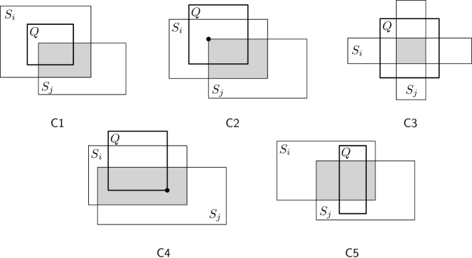
Figure 1: Five configurations of $(S_{i},S_{j})$ and $Q$.

Observation 1 (Five Configurations of Intersections.)

For any pair $(S_{i},S_{j})$ of rectangles of $\mathcal{S}$ with $I(i,j)\cap Q\neq\emptyset$, one of the followings holds. Figure 1 gives an illustration.

• C1. $S_{i}$ or $S_{j}$ contains $Q$.

• C2. $Q$ contains an endpoint of a stretch of $S_{i}$ or $S_{j}$ which is a corner of $I(i,j)$.

• C3. A stretch of $S_{i}$ and a stretch of $S_{j}$ cross $Q$ in different directions.

• C4. $I(i,j)$ contains a corner of $Q$.

• C5. $I(i,j)$ and $Q$ cross each other.

We consider the configurations one by one in our query algorithm. We first report all pairs satisfying C1 (simply, all C1-pairs), then we report all pairs satisfying C2 (simply, all C2-pairs), and so on. There might be a pair $(S_{i},S_{j})$ of input rectangles that belongs to more than one configuration. To avoid reporting the same pair more than once, we give a priority order to the configurations such that our algorithm reports a pair exactly once in the configuration of the highest priority among the configurations the pair belongs to. Since there are only five configurations and we can check in constant time whether a pair belongs to a configuration or not, this does not increase the asymptotic time complexity of our algorithm.

2.2 Reporting All Pairs, except C5-pairs

We first show how to construct data structures for finding all pairs $(S_{i},S_{j})$ of input rectangles with $I(i,j)\cap Q\neq\emptyset$, except C5-pairs. In Section 2.3, we show how to find all C5-pairs.

2.2.1 Data Structures

We construct four data structures for four different problems: the orthogonal segment intersection problem, the point enclosure problem, the orthogonal range reporting problem, and the rectangle crossing problem. There has been a fair amount of work on these problems. We observe that the last problem reduces to the 3D orthogonal range reporting problem with a four-sided query box, which has also been studied well. Thus we use data structures for these four problems after slightly modifying them to achieve our purpose.

Orthogonal Segment Intersection Problem: SegInt.

The orthogonal segment intersection problem asks to preprocess horizontal input segments so that given a query of a vertical segment, the horizontal input segments intersected by the query can be computed efficiently. Chazelle [4] gave a data structure called the hive-graph to solve this problem efficiently. The hive-graph is a planar orthogonal graph with $O(N)$ cells, each of which has a constant number of edges on its boundary, where $N$ is the number of the input segments.

The query algorithm first finds the cell of the hive-graph containing an endpoint of the query segment and traverses the hive-graph along the query segment from the endpoint to the other endpoint. All horizontal edges intersected by the query are encountered during the traversal. In this way, the algorithm finds all horizontal segments intersected by the query in order sorted along the query. The query algorithm takes constant time per output segment, excluding the time for the point location for an endpoint of the query.

In our problem, we construct two hive-graph data structures, one for the horizontal sides of the rectangles of $\mathcal{S}$ and one for the vertical sides of the rectangles of $\mathcal{S}$. The query segments used in our query algorithm are stretches of $\mathcal{S}_{\ell}$. To save the time for point locations in the query algorithm, for each endpoint of the stretches of $\mathcal{S}_{\ell}$, we find the two cells of the two hive-graphs that contain the endpoint in the preprocessing phase. Due to this preprocessing, we can find the sides of the rectangles of $\mathcal{S}$ crossed by a stretch $\ell$ of $\mathcal{S}_{\ell}$ in the sorted order along $\ell$ from one endpoint of $\ell$ in constant time per output side. We denote this data structure by SegInt.

Point Enclosure Problem: PtEnc and EPtEnc.

The point enclosure problem asks to preprocess input rectangles so that all input rectangles containing a query point can be computed efficiently. Chazelle [4] gave a data structure for this problem. We construct this data structure on $\mathcal{S}$ in the preprocessing time, and denote the data structure by PtEnc. It has size $O(n)$ and allows us to find all rectangles of $\mathcal{S}$ containing a query point in $O(\log n+K)$ time, where $K$ is the size of the output in this subproblem. Moreover, it allows us to check whether there exists such a rectangle in $O(\log n)$ time.

In our query algorithm, we consider this problem for two different purposes: finding all rectangles of $\mathcal{S}$ containing a corner of $Q$, and finding all rectangles of $\mathcal{S}$ containing an endpoint of a stretch of $\mathcal{S}_{\ell}$. We perform the former task at most four times in our query algorithm since $Q$ has four corners. Thus we simply use PtEnc for this task. However, we will perform the latter task $\Theta(k)$ times in the worst case, which takes $\Omega(k\log n)$ time. Here $k$ is the size of the output in our query algorithm. Note that we have the endpoints of the stretches of $\mathcal{S}_{\ell}$ in the preprocessing phase, and therefore the latter task can be done in the preprocessing phase.

To do this, we show how the data structure by Chazelle [4] works. Its primary structure is a balanced binary search tree on the rectangles of $\mathcal{S}$ with respect to the $x$-coordinates of their vertical sides. Each node of the binary search tree corresponds to a vertical line, and it is augmented by the hive-graph on the set of the rectangles of $\mathcal{S}$ intersecting its corresponding vertical line. The query algorithm finds $O(\log n)$ nodes of the binary search tree, and then searches on the hive-graphs associated with the nodes. This takes $O(\log n+K)$ time due to fractional cascading, where $K$ is the size of the output in this subproblem.

This means that we consider $O(\log n)$ hive-graphs and spend $O(\log n)$ time to find the cell containing a query point on one hive-graph. The point location on the other hive-graphs can be done by fractional cascading. To save the $\log n$ term in the running time of the query algorithm, we find the cells of the $O(\log n)$ hive-graphs containing each endpoint of the stretches of $\mathcal{S}_{\ell}$ in the preprocessing time. We need $O(n\log n)$ space to store the cells containing endpoints of the stretches of $\mathcal{S}_{\ell}$. Due to the preprocessing, given an endpoint of a stretch of $\mathcal{S}_{\ell}$, we can find all rectangles of $\mathcal{S}$ containing the endpoint in $O(1+K)$ time. Note that $O(1+K)=O(K)$ since each endpoint is contained in at least two rectangles of $\mathcal{S}$, and thus $K>1$. We denote this data structure (PtEnc associated with pointers for the endpoints of the stretches) by EPtEnc.

Orthogonal Range Reporting Problem: RecEnc.

We want to preprocess all endpoints of the stretches of $\mathcal{S}_{\ell}$ so that the endpoints contained in a query rectangle can be computed efficiently. Chazelle [4] presented a data structure for this problem that has $O(n\log n/\log\log n)$ size and supports $O(\log n+K)$ query time, where $K$ is the size of the output. We denote this data structure by RecEnc.

Rectangle Crossing Problem: RecCross and RecInt.

We want to preprocess the stretches of $\mathcal{S}_{\ell}$ so that all stretches crossing a query rectangle can be computed efficiently. De Berg et al. [8] also considered this problem. To do this, they reduce this problem to the orthogonal range reporting problem in three dimensional space as follows. Let $[a,b]\times[c,d]$ be a query rectangle. The query rectangle is crossed by a vertical stretch $x_{1}\times[y_{1},y_{2}]$ if and only if $x_{1}\in[a,b]$, $y_{1}\in[-\infty,c]$, and $y_{2}\in[d,\infty]$. Using this observation, they map each vertical stretch $x_{1}\times[y_{1},y_{2}]$ to the point $(x_{1},y_{1},y_{2})$ in $\mathbb{R}^{3}$. Then we can find all vertical stretches crossing the query rectangle by finding all points contained in the orthogonal region $[a,b]\times[-\infty,c]\times[d,\infty]$. Similarly, we can do this for horizontal stretches. However, they did not use the fact that a query is unbounded: it is four-sided in $\mathbb{R}^{3}$. In this case, we can use a more efficient algorithm given by Afshani et al. [1] instead of the one in [12]. In fact, this is also mentioned in the journal paper [7] by the authors, which has been available online recently. The algorithm by Afshani et al. takes $O(\log n+K)$ time for four-sided query boxes using a data structure of $O(n\log n/\log\log n)$ size, where $K$ is the size of the output. We denote this data structure by RecCross. This data structure has size $O(n\log n/\log\log n)$ and allows us to find all vertical (or horizontal) stretches of $\mathcal{S}_{\ell}$ crossing a query rectangle in $O(\log n+K)$ time, where $K$ is the size of the output.

A rectangle $S$ of $\mathcal{S}$ intersects a query rectangle $Q$ if and only if (1) $Q$ crosses a side of $S$, (2) $Q$ contains a corner of $S$, or (3) $Q$ is contained in $S$. To find all rectangles of $\mathcal{S}$ intersecting a query rectangle, we use RecCross for case (1), use RecEnc for case (2), and use PtEnc for case (3). We call the combination of these data structures RecInt. We can find all rectangles of $\mathcal{S}$ intersecting $Q$ in $O(\log n+K)$ time using RecInt, where $K$ is the size of the output in this subproblem.

2.2.2 Query Algorithms.

Assume that we have the data structures of size $O(n\log n)$ described in Section 2.2.1. Then, we can find all pairs $(S_{i},S_{j})$ of $\mathcal{S}$ with $I(i,j)\cap Q\neq\emptyset$, except C5-pairs, in $O(\log n+k)$ time.

Reporting C1-pairs of $Q$.

We can find the C1-pairs of $Q$ in $O(\log n+k(Q))$ time. A pair of rectangles of $\mathcal{S}$ is a C1-pair of $Q$ if one rectangle of the pair contains all four corners of $Q$ and the other rectangle intersects $Q$.

We find the rectangles of $\mathcal{S}$ containing all four corners of $Q$ by finding all rectangles of $\mathcal{S}$ containing each corner of $Q$ using PtEnc. Note that there are $O(k(Q)+1)$ rectangles that contain a corner of $Q$ simply because every pair of the rectangles containing the corner is in $\mathcal{U}(Q)$. (We need “$+1$” since it is possible that there is just one rectangle containing the corner, but $k(Q)$ is zero.) Thus, we can compute such rectangles in $O(\log n+k(Q))$ time. Let $\mathcal{S}_{1}$ denote the set of all rectangles containing all four corners of $Q$.

If $\mathcal{S}_{1}$ is not empty, we find all rectangles intersecting $Q$ in $O(\log n+K)$ time using RecInt, where $K$ is the number of such rectangles. Since $\mathcal{S}_{1}$ is not empty, $K$ is at most $k(Q)$. Let $\mathcal{S}_{2}$ be the set of all rectangles intersecting $Q$. We report every pair $(S_{1},S_{2})$ with $S_{1}\in\mathcal{S}_{1}$ and $S_{2}\in\mathcal{S}_{2}$ as a C1-pair of $Q$, which takes $O(\log n+k(Q))$ time. It is clear that we report all C1-pairs of $Q$ in this way.

Reporting C2-pairs of $Q$.

We can find the C2-pairs of $Q$ in $O(\log n+k(Q))$ time. A pair of rectangles of $\mathcal{S}$ is a C2-pair of $Q$ if $Q$ contains an endpoint of a stretch $\ell$ of one of them and the other intersects $\ell\cap Q$. We find all stretches of $\mathcal{S}_{\ell}$ whose endpoints are in $Q$ in $O(\log n+k(Q))$ time using RecEnc. The number of such stretches is $O(k(Q))$ because each endpoint of the stretches of $\mathcal{S}_{\ell}$ is contained in at least two rectangles of $\mathcal{S}$ and there are at most four stretches from one rectangle of $\mathcal{S}$.

For each stretch $\ell$ with an endpoint in $Q$, we want to find all rectangles $S$ of $\mathcal{S}$ with $S\cap\ell\cap Q\neq\emptyset$. Such rectangles $S$ satisfy one of the followings: $\ell\cap Q$ is intersected by the boundary of $S$ or $\ell\cap Q$ is contained in $S$. For the former case, we use SegInt. Starting from the endpoint of $\ell$ contained in $Q$, we traverse the hive-graph along $\ell$ until we escape from $Q$ or we arrive at the other endpoint of $\ell$. We find all rectangles $S$ whose sides intersect $\ell\cap Q$ in time linear in the number of such rectangles using SegInt. For the latter case, we compute all rectangles containing the endpoint of $\ell$ that is also in $Q$ in time linear in the number of such rectangles using EPtEnc. Therefore, for each stretch $\ell$ with an endpoint in $Q$, we can find all rectangles of $\mathcal{S}$ intersecting $\ell\cap Q$ in time linear in the number of such rectangles.

By applying this procedure for every stretch with an endpoint in $Q$, we can find all C2-pairs of $Q$ in $O(k(Q))$ time, excluding the time for finding all such stretches. Therefore, we can compute all C2-pairs of $Q$ in $O(\log n+k(Q))$ time in total.

Reporting C3-pairs of $Q$.

We can find the C3-pairs of $Q$ in $O(\log n+k(Q))$ time. A pair of rectangles of $\mathcal{S}$ is a C3-pair of $Q$ if two stretches, one from each rectangle, cross $Q$ in different directions. Let $\mathcal{S}_{v}$ be the set of the rectangles of $\mathcal{S}$ whose vertical stretches cross $Q$. Let $\mathcal{S}_{h}$ be the set of the rectangles of $\mathcal{S}$ whose horizontal stretches cross $Q$.

We first check whether $\mathcal{S}_{v}$ or $\mathcal{S}_{h}$ is empty in $O(\log n)$ time using RecCross. If one of them is empty, there is no C3-pair of $Q$. If both of them are nonempty, we compute $\mathcal{S}_{v}$ and $\mathcal{S}_{h}$ in $O(\log n+k(Q))$ time using RecCross. The size of $\mathcal{S}_{v}$ and $\mathcal{S}_{h}$ is $O(k(Q))$ since every rectangle of $\mathcal{S}_{v}$ intersects every rectangle of $\mathcal{S}_{h}$ in $Q$. Then we report the pairs $(S,S^{\prime})$ with $S\in\mathcal{S}_{v}$ and $S^{\prime}\in\mathcal{S}_{h}$ as the C3-pairs in $O(\log n+k(Q))$ time in total.

Reporting C4-pairs of $Q$.

We can report the C4-pairs of $Q$ in $O(\log n+k(Q))$ time. A pair of rectangles of $\mathcal{S}$ is a C4-pair of $Q$ if the intersection of the rectangles contains a corner of $Q$. In this case, both rectangles of the pair contains a corner of $Q$. We first check whether there exists a rectangle of $\mathcal{S}$ containing a corner of $Q$ in $O(\log n)$ time using PtEnc. Again, the number of the rectangles of $\mathcal{S}$ containing a corner of $Q$ is $O(k(Q))$ as every pair of such rectangles is in $\mathcal{U}(Q)$. If there exists a rectangle containing a corner of $Q$, we find all rectangles containing the corner of $Q$ in $O(\log n+k(Q))$ time using PtEnc. Then we report all pairs consisting of the rectangles containing the corner of $Q$. We do this for each of the other corners of $Q$. Then we can report all C4-pairs in $O(\log n+k(Q))$ time.

2.3 Reporting C5-pairs

We have shown how to find all pairs of rectangles of $\mathcal{S}$ intersecting each other in $Q$, except for the C5-pairs. There might be some pairs of rectangles that belong to both C5 and one of the other configurations. As mentioned earlier, this can be checked in constant time per pair of rectangles. Since we use a priority order over the configurations, we assume that they have already been reported by the algorithm for the configurations other than C5.

A pair of rectangles of $\mathcal{S}$ is a C5-pair of a query rectangle $Q$ if the intersection of the rectangles and $Q$ cross each other. In the following, we show how to find and report the C5-pairs of $Q$ not belonging to any other configuration such that the horizontal sides of the intersection intersect the vertical sides of $Q$. The C5-pairs not belonging to any other configuration such that the vertical sides of the intersection intersect the horizontal sides of $Q$ can be found analogously.

One-Dimensional Segment Tree.

We construct a one-dimensional segment tree $T$ of $\mathcal{S}$ with respect to the $x$-axis as follows [6]. The segment tree is a balanced binary search tree on the orthogonal projections of the rectangles of $\mathcal{S}$ onto the $x$-axis. Each node $v$ of the balanced binary search tree corresponds to a closed vertical slab $H(v)$. The union of all vertical slabs corresponding to the nodes at the same level is $\mathbb{R}^{2}$. We say that a rectangle $S$ crosses $H(v)$ if $S$ intersects $H(v)$ and no vertical side of $S$ is contained in $H(v)$. Let $\mathcal{S}_{C}(v)$ be the set of the rectangles of $\mathcal{S}$ that cross $H(v)$ but do not cross $H(u)$ for the parent $u$ of $v$ in $T$. There are $O(\log n)$ nodes $v$ with $S\in\mathcal{S}_{C}(v)$ for a rectangle $S$. Moreover, the union of $H(v)$’s for all such nodes $v$ contains $S$. Let $\mathcal{S}_{B}(v)$ be the set of the rectangles of $\mathcal{S}$ whose left or right side is contained in the interior of $H(v)$. Note that $\mathcal{S}_{B}(v)$ is empty for every leaf node $v$. For a rectangle $S\in\mathcal{S}$, there are at most two nodes $v$ of $T$ with $S\in\mathcal{S}_{B}(v)$ at each level of $T$, and each such node lies on one of the two paths of $T$ from the root to two leaf nodes $w,w^{\prime}$ with the left side of $S$ contained in $H(w)$ and the right side of $S$ contained in $H(w^{\prime})$. We use $\mathcal{S}(v)$ to denote the union of $\mathcal{S}_{C}(v)$ and $\mathcal{S}_{B}(v)$. For each node $v$ of $T$, we store $\mathcal{S}_{B}(v)$ and $\mathcal{S}_{C}(v)$. The binary search tree together with the sets $\mathcal{S}_{B}(\cdot)$ and $\mathcal{S}_{C}(\cdot)$ forms the segment tree of $\mathcal{S}$. The size of $T$ is $O(n\log n)$.

Canonical Nodes of a C5-pair.

Consider any C5-pair $(S_{i},S_{j})$ of $Q$. There are $O(\log n)$ nodes $v$ of $T$ such that $S_{i},S_{j}\in\mathcal{S}(v)$ and $I(i,j)\cap Q\cap H(v)\neq\emptyset$. This means that there can be $\Omega(k\log n)$ such nodes in the worst case for all C5-pairs in total. Instead of considering all of them, we use canonical nodes (to be defined below) such that there is a unique canonical node of $(i,j,Q)$ in $T$ for any C5-pair. We will show how to find the canonical nodes and report all C5-pairs efficiently in the subsequent sections. See Figure 2.

Definition 2

For a rectangle $Q$ and a pair $(S_{i},S_{j})$ of the rectangles of $\mathcal{S}$ with $I(i,j)\cap Q\neq\emptyset$, a node $v$ of $T$ is called the canonical node of $(i,j,Q)$ if the left side of $Q$ is contained in $H(v)$ and both $S_{i}$ and $S_{j}$ are in $\mathcal{S}(v)$ satisfying $S_{i}\in\mathcal{S}_{C}(v)$ or $S_{j}\in\mathcal{S}_{C}(v)$.

Note that not every canonical node of some triple $(i,j,Q)$ defines a C5-pair of $Q$, though $I(i,j)\cap Q\neq\emptyset$. However, there is a canonical node of $(i,j,Q)$ in $T$ for each C5-pair of $Q$ such that the horizontal sides of $I(i,j)$ intersect the vertical sides of $Q$.

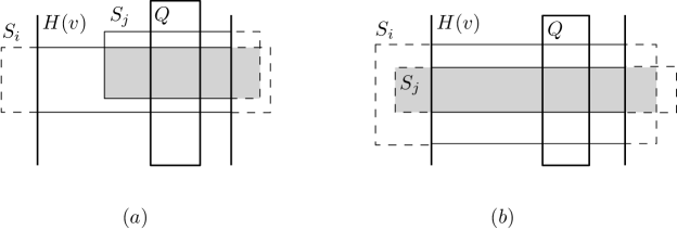
Figure 2: (a) A canonical node $v$ of $(i,j,Q)$. It holds that $S_{i}\in\mathcal{S}_{C}(v)$ and $S_{j}\in\mathcal{S}_{B}(v)$. (b) A canonical node $v$ of $(i,j,Q)$. It holds that both $S_{i}$ and $S_{j}$ are in $\mathcal{S}_{C}(v)$.

Lemma 3

For any C5-pair $(S_{i},S_{j})$ of $Q$ such that the horizontal sides of $I(i,j)$ intersect the vertical sides of $Q$, there is a canonical node of $(i,j,Q)$ in $T$.

Proof.  Consider the C5-pairs of $Q$ such that the horizontal sides of the intersection intersects the vertical sides of $Q$. Let $p$ be the intersection between the left side of $Q$ and the top side of $I(i,j)$. Then there is a path $\pi$ from the root node to some leaf node $u$ with $p\in H(u)$ in $T$. Consider a node $w$ in $\pi$. Since $p$ lies on the left side of $Q$, the slab $H(w)$ contains the left side of $Q$. Moreover, $H(w)$ intersects both $S_{i}$ and $S_{j}$.

We claim that there is a canonical node of $(i,j,Q)$ in $\pi$. By the construction of the segment tree, $S_{i}\in\mathcal{S}_{B}(v)$ for the root node $v$ and $S_{i}\not\in\mathcal{S}_{B}(u)$ for the leaf node $u$ of $\pi$. Thus, there is a node $w_{i}$ of $\pi$ with $S_{i}\in\mathcal{S}_{C}(w_{i})$. For a node $w$ closer to the root node than $w_{i}$, $S_{i}\in\mathcal{S}_{B}(w)$. For a node $w^{\prime}$ closer to the leaf node than $w_{i}$ along $\pi$, $S_{i}\not\in\mathcal{S}(w^{\prime})$. This also holds for $S_{j}$, so there is a node $w_{j}$ of $\pi$ with $S_{j}\in\mathcal{S}_{C}(w_{j})$. Without loss of generality, we assume that $w_{i}$ lies between the root node and $w_{j}$ (including them) along $\pi$. Then we have $S_{i}\in\mathcal{S}_{C}(w_{i})$ and $S_{j}\in\mathcal{S}(w_{i})$. Since $w_{i}$ is in $\pi$, $H(w_{i})$ contains the left side of $Q$. Therefore, $w_{i}$ is a canonical node of $(i,j,Q)$ in $\pi$.    

We need the following lemma to bound the total number of canonical nodes for $Q$ over all pairs of rectangles of $\mathcal{S}$ by $O(k(Q))$. Notice that the following lemma holds for a pair of rectangles of any configuration from C1 to C5.

Lemma 4

For any rectangle $Q$ and any pair $(S_{i},S_{j})$ of rectangles of $\mathcal{S}$ with $I(i,j)\cap Q\neq\emptyset$, there is at most one canonical node of $(i,j,Q)$ in $T$.

Proof.  Let $v$ be a canonical node of $(i,j,Q)$ in $T$. Since the left side of $Q$ is contained in $H(v)$, the node $v$ is in the path $\pi$ of $T$ from the root node to the leaf node $u$ such that the left side of $Q$ is contained in $H(u)$. By the construction of the segment tree, there is at most one node $w_{i}$ on $\pi$ with $S_{i}\in\mathcal{S}_{C}(w_{i})$, and there is at most one node $w_{j}$ on $\pi$ with $S_{j}\in\mathcal{S}_{C}(w_{j})$. Therefore, no node of $T$ other than $w_{i}$ and $w_{j}$ is a canonical node of $(i,j,Q)$.

Without loss of generality, we assume that $v=w_{i}$. Then we have $S_{j}\in\mathcal{S}(w_{i})$ by the definition of the canonical node. If $S_{j}\in\mathcal{S}_{C}(w_{i})$, we have $w_{i}=w_{j}$ and $w_{i}$ is the unique canonical node. If $S_{j}\in\mathcal{S}_{B}(w_{i})$, $w_{j}$ is not a canonical node of $(i,j,Q)$ because $w_{i}$ lies between the root node and $w_{j}$ (including the root node) along $\pi$ and $S_{i}\notin\mathcal{S}(w_{j})$. Therefore, there is at most one canonical node of $(i,j,Q)$.    

Corollary 5

The total number of canonical nodes for a query rectangle $Q$ is $O(k(Q))$.

Our general strategy is the following. Given a query rectangle $Q$, we find a set of nodes of the segment tree $T$ that contains the canonical node of $(i,j,Q)$ for every C5-pair $(S_{i},S_{j})$ not belonging to any other configuration such that the horizontal sides of $I(i,j)$ intersect the vertical sides of $Q$ in $O(\log n+k(Q))$ time. The size of this set is $O(k(Q))$. For each such node $v$, we find all C5-pairs $(S_{i},S_{j})$ such that $v$ is a canonical node of $(i,j,Q)$ in time linear in the number of the output.

2.3.1 Finding All Canonical Nodes for C5-pairs

In this subsection, we present data structures and their query algorithms to find a set of canonical nodes of $(i,j,Q)$ with $I(i,j)\cap Q\neq\emptyset$ for a query rectangle $Q$. This set contains the canonical node of $(i,j,Q)$ for every C5-pair $(S_{i},S_{j})$ not belonging to any other configuration. We show how to do this for the C5-pairs such that the horizontal sides of $I(i,j)$ intersect the vertical sides of $Q$.

Data Structures.

For each node $v$ of $T$ and each rectangle $S$ of $\mathcal{S}(v)$, we define the trimmed rectangle for $(S,v)$ as the smallest rectangle containing $S_{v}\cap U(v)$, where $S_{v}=S\cap H(v)$ and $U(v)=\bigcup_{S^{\prime}\in\mathcal{S}_{C}(v)}S^{\prime}$. See Figure 3 for an illustration.

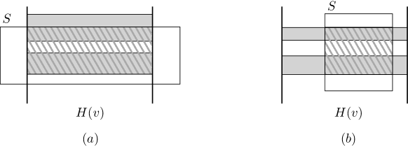
Figure 3: A node $v$ and a rectangle $S\in\mathcal{S}(v)$. The gray regions represent $H(v)\cap\bigcup_{S^{\prime}\in\mathcal{S}_{C}(v)}S^{\prime}$. (a) The trimmed rectangle (dashed region) for $(S,v)$ with $S\in\mathcal{S}_{C}(v)$. (b) The trimmed rectangle (dashed region) for $(S,v)$ with $S\in\mathcal{S}_{B}(v)$.

Let $\mathcal{L}$ be the set of the horizontal sides of all trimmed rectangles for all nodes of $T$. Note that $|\mathcal{L}|=O(n\log n)$. To compute $\mathcal{L}$ efficiently, we sort the rectangles of $\mathcal{S}$ in decreasing order with respect to their top sides in $O(n\log n)$ time. This allows us to sort all rectangles of $\mathcal{S}(v)$ for each node $v$ of $T$ in the same depth in $O(n)$ time in total. Therefore, we can sort the rectangles of $\mathcal{S}(v)$ in decreasing order with respect to their top sides for every node $v$ of $T$ in $O(n\log n)$ time in total. Similarly, we sort the rectangles of $\mathcal{S}_{C}(v)$ for every node $v$ of $T$ in $O(n\log n)$ time. The trimmed rectangle for $(S,v)$ is $S\cap H(v)$ for a rectangle $S$ of $\mathcal{S}_{C}(v)$. For a rectangle $S$ of $\mathcal{S}_{B}(v)$, the top side of the trimmed rectangle for $(S,v)$ is the highest top side of the rectangles of $\mathcal{S}_{C}(v)$ lying below the top side of $S$ if the top side of $S$ is not contained in any rectangle of $\mathcal{S}_{C}(v)$. Otherwise, the top side of the trimmed rectangle is the top side of $S$. Therefore, the top sides of the trimmed rectangles for $(S,v)$ can be computed in $O(|\mathcal{S}(v)|)$ time for a node $v$ of $T$ and all rectangles $S\in\mathcal{S}(v)$. Thus we can compute $\mathcal{L}$ in time linear in its size, which is $O(n\log n)$.

We construct the hive-graph on $\mathcal{L}$, which allows us to report all horizontal sides of $\mathcal{L}$ intersecting a query vertical segment $\ell$ in sorted order along $\ell$ in $O(\log n+K)$ time, where $K$ is the size of output [4]. Since the size of $\mathcal{L}$ is $O(n\log n)$, the hive-graph has $O(n\log n)$ size. We make each segment of $\mathcal{L}$ to point to the rectangle of $\mathcal{S}$ from which the segment comes.

Query Algorithm.

Given a query rectangle $Q$, our query algorithm finds all sides of $\mathcal{L}$ intersecting the left side of $Q$ using the hive-graph on $\mathcal{L}$. Then for each such side, our query algorithm marks the node of $T$ pointed by the side as a canonical node in $O(\log n+k)$ time due to the following lemmas.

Lemma 6

The query algorithm finds the canonical node of $(i,j,Q)$ for every C5-pair $(S_{i},S_{j})$ not belonging to any other configuration such that the horizontal sides of $I(i,j)$ intersect the vertical sides of $Q$.

Proof.  Consider a C5-pair $(S_{i},S_{j})$ of $Q$ not belonging to any other configurations such that the horizontal sides of $I(i,j)$ intersect the vertical sides of $Q$. There is a unique canonical node $v$ of $(i,j,Q)$ by Lemma 3 and Lemma 4. Let $S_{i}^{\prime}$ and $S_{j}^{\prime}$ be the trimmed rectangles for $(S_{i},v)$ and $(S_{j},v)$, respectively.

We claim that a horizontal side of $S_{j}$ is intersected by the left side of $Q$. Since $(S_{i},S_{j})$ belongs to C5, the left side of $S_{j}$ lies to the left of $Q$, and the right side of $S_{j}$ lies to the right of $Q$. There are only two cases to consider: a horizontal side of $S_{j}$ is intersected by the left side of $Q$, or $S_{j}$ contains $Q$. For the second case, $(S_{i},S_{j})$ belongs to C1. This contradicts the assumption that $(S_{i},S_{j})$ does not belong to any configuration other than C5. Thus the only possible case is the first one, and the claim holds.

Now we claim that a horizontal side of $S_{j}^{\prime}$ is intersected by the left side of $Q$, and thus the query algorithm finds $v$ as the canonical node of $(i,j,Q)$. Without loss of generality, we assume that the top side of $S_{j}$ is intersected by the left side of $Q$. The top side of $S_{j}^{\prime}$ lies in between the top side of $S_{j}$ and the top side of $I(i,j)$. Since the top side of $S_{j}$ and the top side of $I(i,j)$ intersects the left side of $Q$, the claim holds.    

Lemma 7

The number of the sides of $\mathcal{L}$ intersecting the left side of $Q$ is $O(k(Q))$.

Proof.  We use a charging scheme as follows. We charge each horizontal side $\ell$ of $\mathcal{L}$ intersecting the left side $\ell_{Q}$ of $Q$ to a pair $(S_{i},S_{j})\in\mathcal{U}(Q)$ with $S_{i}\in\mathcal{S}_{C}(v)$ and $S_{j}\in\mathcal{S}(v)$ such that both $S_{i}$ and $S_{j}$ contain the intersection point of $\ell$ and $\ell_{Q}$. If there are more than one such pair, we charge $\ell$ to an arbitrary one.

We claim that there exists such a pair for every horizontal side of $\mathcal{L}$ intersecting the left side of $Q$. Consider a horizontal side $\ell$ of $\mathcal{L}$. Let $S_{j}$ be the rectangle of $\mathcal{S}$ defining $\ell$. In other words, let $S_{j}$ be a rectangle of $\mathcal{S}$ such that the trimmed rectangle $S_{j}^{\prime}$ for $(S_{j},v)$ has $\ell$ as its horizontal side for some node of $T$. By the definition of the trimmed rectangle, a horizontal side of $S_{j}^{\prime}$ is contained in some rectangle of $\mathcal{S}_{C}(v)$, say $S_{i}$. Thus, the intersection of the horizontal side of $S_{j}^{\prime}$ and the left side of $Q$ is contained in $S_{i}$. This means that $(S_{i},S_{j})\in\mathcal{U}(Q)$.

Now we claim that each pair $(S_{i},S_{j})\in\mathcal{U}(Q)$ is charged at most once in this way. In each node $v$, a pair $(S_{i},S_{j})$ is charged at most once. Moreover, $(S_{i},S_{j})$ is charged only in the canonical node of $(i,j,Q)$, which is unique by Lemma 4. Therefore, $(S_{i},S_{j})$ is charged at most once, and the lemma holds.    

Lemma 8

Given a query rectangle $Q$, we can find a set of at most $k$ nodes of $T$ containing all canonical nodes for C5-pairs not belonging to any other configuration in $O(\log n+k)$ time.

2.3.2 Handling Each Canonical Node to Find All C5-pairs

Let $\mathcal{V}_{Q}$ be the set of all nodes we found in Section 2.3.1. For each node $v\in\mathcal{V}_{Q}$, we show how to find all C5-pairs $(S_{i},S_{j})$ not belonging to any other configuration such that $v$ is a canonical node of $(i,j,Q)$. Here, we consider only the case that $S_{i}\in\mathcal{S}_{C}(v)$ and $S_{j}\in\mathcal{S}(v)$. The other case that $S_{j}\in\mathcal{S}_{C}(v)$ and $S_{i}\in\mathcal{S}(v)$ can be handled analogously. Moreover, we consider only the C5-pairs such that the horizontal sides of $I(i,j)$ intersect the vertical sides of $Q$. The other case can be handled analogously.

For each node $v$, we spend $O(1+k(v))$ time, where $k(v)$ is the number of the pairs $(S_{i},S_{j})$ with $I(i,j)\cap Q\neq\emptyset$ such that $v$ is a canonical node of $(i,j,Q)$. Note that the sum of $k(v)$ for every node $v$ of $\mathcal{V}_{Q}$ is $O(k)$ by Lemma 4. Once we do this for every node in $\mathcal{V}_{Q}$, we can obtain all C5-pairs for the canonical nodes of $(i,j,Q)$ not belonging to any other configuration in $O(k)$ time, excluding the time for computing all such canonical nodes.

Overall Strategy.

Let $\mathcal{S}_{Q}$ be the set of all rectangles $S_{j}\in\mathcal{S}(v)$ for each node $v\in\mathcal{V}_{Q}$ such that a horizontal side of the trimmed rectangle for $(S_{j},v)$ intersects the left side of $Q$. We obtain $\mathcal{S}_{Q}$ while computing the set $\mathcal{V}_{Q}$ in Section 2.3.1. Consider a C5-pair $(S_{i},S_{j})$ not belonging to any other configuration such that the horizontal sides of $I(i,j)$ intersect the vertical side of $Q$. The proof of Lemma 6 shows that a horizontal side of the trimmed rectangle for $(S_{j},v)$ is intersected by the left side of $Q$, where $v$ is the canonical node of $(i,j,Q)$. This means that $S_{j}$ is in $\mathcal{S}_{Q}$. Since we already have $S_{j}$, the remaining task is to find $S_{i}$.

Given a node $v\in\mathcal{V}_{Q}$ and a rectangle $S_{j}$ in $\mathcal{S}_{Q}\cap\mathcal{S}_{C}(v)$, we are to compute all rectangles $S_{i}\in\mathcal{S}(v)$ with $I(i,j)\cap Q\neq\emptyset$. For a rectangle $S_{i}\in\mathcal{S}(v)$ with $I(i,j)\cap Q\neq\emptyset$, we observe that $\mathsf{y}(S_{j})$, $\mathsf{y}(S_{i})$ and $\mathsf{y}(Q)$ contain a common point, where $\mathsf{y}(A)$ is the the orthogonal projection of a set $A\subseteq\mathbb{R}^{2}$ onto the $y$-axis. There are two cases: $\mathsf{y}(S_{j})\cap\mathsf{y}(Q)$ contains an endpoint of $\mathsf{y}(S_{i})$, or $\mathsf{y}(S_{j})\cap\mathsf{y}(Q)$ is contained in $\mathsf{y}(S_{i})$.

Data Structures and Preprocessing.

We maintain two data structures, one for finding the rectangles of the first case and the other for finding the rectangles of the second case. The first one is organized as follows. For each node $v$ of $T$, we maintain two sorted lists of the rectangles of $\mathcal{S}_{C}(v)$, one with respect to their top sides and the other with respect to their bottom sides. We make each rectangle $S$ of $\mathcal{S}_{B}(v)$ to point to the rectangle of $\mathcal{S}_{C}(v)$ with highest bottom side (and highest top side) lying below the top side (and bottom side) of the trimmed rectangle for $(S,v)$. Similarly, we make $S$ to point to the rectangle of $\mathcal{S}_{C}(v)$ with lowest top side (and lowest bottom side) lying above the bottom side (and top side) of the trimmed rectangle for $(S,v)$.

For the second one, we use a partially persistent data structure of a linked list. Once we update a linked list and destroy the old versions, we cannot search any element on an old version any longer. But a partially persistent data structure allows us to access any version at any time by keeping the changes on the linked list. Driscoll et al. [9] presented a general method to make a data structure based on pointers partially persistent. Using their method, we can construct a partially persistent data structure of a linked list.

In our case, the linked list has rectangles of $\mathcal{S}_{C}(v)$ as its elements. We consider a $y$-coordinate as a time stamp. A rectangle $S\in\mathcal{S}_{C}(v)$ is appended to the linked list at time $t_{1}$ and is deleted from the linked list at time $t_{2}$, where $t_{1}$ is the $y$-coordinate of the top side of $S$ and $t_{2}$ is the $y$-coordinate of the bottom side of $S$. Each insertion and deletion can be done in constant time, which is subsumed in the total preprocessing time. For each horizontal side of $S_{c}\in\mathcal{S}_{C}(v)$, we need an extra pointer that points to the first element of the persistent data structure at time $t$, where $t$ is the $y$-coordinate of the horizontal side. The size of the partially persistent data structure is linear in the size of $\mathcal{S}(v)$. Due to the partially persistent data structure and the pointers associated with the horizontal sides of the rectangles of $\mathcal{S}(v)$, we can find all rectangles of $\mathcal{S}(v)$ containing a horizontal side of $S_{c}\in\mathcal{S}_{C}(v)$ in time linear in the size of the output.

Query Algorithm.

Given a node $v\in\mathcal{V}_{Q}$ and a rectangle $S_{j}$ in $\mathcal{S}_{Q}\cap\mathcal{S}_{C}(v)$, we are to compute all rectangle $S_{i}\in\mathcal{S}(v)$ such that $\mathsf{y}(S_{j})$, $\mathsf{y}(S_{i})$ and $\mathsf{y}(Q)$ contain a common point. Recall that there are two cases: $\mathsf{y}(S_{j})\cap\mathsf{y}(Q)$ contains an endpoint of $\mathsf{y}(S_{i})$, or $\mathsf{y}(S_{j})\cap\mathsf{y}(Q)$ is contained in $\mathsf{y}(S_{i})$. A horizontal side of the trimmed rectangle for $(S_{j},v)$ is intersected by the left side of $Q$ by the definition of $\mathcal{S}_{Q}$. Thus at least one endpoint of $\mathsf{y}(S_{j})$ is contained in $\mathsf{y}(Q)$. We assume that the endpoint of $\mathsf{y}(S_{j})$ with smaller $y$-coordinate is contained in $\mathsf{y}(Q)$. In other words, the bottom side of $S_{j}$ intersects $Q$. The other case can be handled analogously.

To find the rectangles $S_{i}$ belonging to the first case, we do the followings. We search the sorted list of the rectangles of $\mathcal{S}_{C}(v)$ with respect to their top sides starting from the rectangle of $\mathcal{S}_{C}(v)$ with lowest top side lying above the bottom side of $S_{j}$. Note that we can obtain the starting point using the pointer that the bottom side of $S_{j}$ has. We stop searching the sorted list when we reach the top side of $S_{j}$ or the top side of $Q$. In this way, we can find all rectangles $S_{i}$ of $\mathcal{S}_{C}(v)$ belonging to the first case in $O(1+K)$ time, where $K$ is the number of such rectangles.

To find the rectangles $S_{i}$ belonging to the second case, we do the followings. A rectangle $S_{i}$ belonging to the second case intersects the bottom side $\ell$ of $S_{j}$. We search the partially persistent data structure at time $t$, where $t$ is the $y$-coordinate of $\ell$. Specifically, starting from the pointer that $\ell$ points to, we traverse the linked list at time $t$. All rectangles we encounter are the rectangles containing $\ell$. This takes $O(1+K^{\prime})$ time, where $K^{\prime}$ is the number of such rectangles.

In total, we spend $O(1+k(v))$ time for each node $v\in\mathcal{V}_{Q}$, where $k(v)$ is the number of the pairs $(S_{i},S_{j})$ of $\mathcal{U}(Q)$ such that the canonical node of $(i,j,Q)$ is $v$. Note that $k(v)$ is at least one for every node $v\in\mathcal{V}_{Q}$ by the construction of $\mathcal{V}_{Q}$. Once we do this for every node in $\mathcal{V}_{Q}$, we can obtain $\mathcal{U}(Q)$ in $O(1+k(Q))$ time in total.

Lemma 9

Given a query rectangle $Q$, we can find all C5-pairs in $O(\log n+k(Q))$ time.

Therefore, we have the following theorem.

Theorem 10

We can construct a data structure of size $O(n\log n)$ on a set $\mathcal{S}$ of $n$ axis-parallel rectangles so that for a query axis-parallel rectangle $Q$, the pairs $(S_{i},S_{j})$ of $\mathcal{S}$ with $S_{i}\cap S_{j}\cap Q\neq\emptyset$ can be reported in $O(\log n+k)$ time, where $k$ is the size of the output.

3 Higher Dimensional Case

In this section, we consider a set $\mathcal{S}=\{S_{1},\ldots,S_{n}\}$ of $n$ axis-parallel boxes in $\mathbb{R}^{d}$ for a constant $d>2$. Let $\delta\in\mathbb{R}$ be any constant with $1/d\leq\delta<1$. We present a data structure that supports $O(n^{1-\delta}\log^{d-1}n+k\operatorname{polylog}n)$ query time. The size of the data structure is $O(n^{\delta d-2\delta+1}\log n)$. There has been no known result for this problem in higher dimensions, except that for $d=3$, the best known data structure has size of $O(n\sqrt{n}\log n)$ and supports $O(\sqrt{n}\log^{2}n+k\log^{2}n)$ query time [7].

3.1 Data Structure

We denote the $t$th axis of $\mathbb{R}^{d}$ by the $\mathsf{x}_{t}$-axis for $1\leq t\leq d$. The $\mathsf{x}_{t}$-projection of a point set $A\subseteq\mathbb{R}^{d}$ is defined as the orthogonal projection of $A$ onto the $\mathsf{x}_{t}$-axis. A box is given in the form $\{(\mathsf{x}_{1},\mathsf{x}_{2},\ldots,\mathsf{x}_{d})\mid a_{t}\leq\mathsf{x}_{t}\leq b_{t},1\leq t\leq d\}$ and has $2d$ facets. We call a facet of the box orthogonal to the $\mathsf{x}_{t}$-axis an $\mathsf{x}_{t}$-facet of the box for any $1\leq t\leq d$. Our data structure consists of the following substructures. We denote the combination of them by $\textsc{BoxPairInt}[d]$.

$n^{\delta}$-Clustered Grid Cells.

For each index $1\leq t\leq d$, we construct $O(n^{\delta})$ intervals on the $\mathsf{x}_{t}$-axis. Consider the $\mathsf{x}_{t}$-projection of the $\mathsf{x}_{t}$-facets of the boxes of $\mathcal{S}$, which forms $2n$ points on $\mathsf{x}_{t}$. We choose every $\lfloor n^{1-\delta}\rfloor$th points in the projection. Then we have $O(n^{\delta})$ points in the projection that define $O(n^{\delta})$ intervals containing no chosen points in its interior. Let $\mathcal{I}_{t}$ be the set of such intervals. A grid cell is a $d$-tuple $(I_{1},\ldots,I_{d})$ of intervals $I_{t}\in\mathcal{I}_{t}$ for $1\leq t\leq d$. Note that there are $O(n^{\delta d})$ grid cells. For a box $B$ in $\mathbb{R}^{d}$, not necessarily in $\mathcal{S}$, we call the grid cell containing the corner of $B$ with minimum $\mathsf{x}_{t}$-coordinates for all $1\leq t\leq d$ the canonical grid cell of a box $B$. Every box in $\mathbb{R}^{d}$ has a unique canonical grid cell.

Grid Containment Data Structure: GridCont.

We mark a grid cell if it is the canonical grid cell of $I(i,j)$ for a pair $(S_{i},S_{j})$. We construct the grid containment data structure on the marked grid cells, denoted by GridCont, that allows us to find all marked grid cells contained in a query axis-parallel box. To do this, we compute the largest box $Q^{\prime}$ contained in $Q$ and aligned to the grid in $O(d\log n)$ time. Specifically, for each $1\leq t\leq d$, we compute the union of all intervals of $\mathcal{I}_{t}$ on the $\mathsf{x}_{t}$-axis contained in the $\mathsf{x}_{t}$-projection of $Q$ in $O(\log n)$ time by applying binary search on the intervals of $\mathcal{I}_{t}$. Then $Q^{\prime}$ is the box whose $\mathsf{x}_{t}$-projection is the union on the $\mathsf{x}_{t}$-interval for every $1\leq t\leq d$. Then it suffices to find every marked grid cell having its corner contained in $Q^{\prime}$. We construct a data structure of size $O(n(\log n/\log\log n)^{d-1})$ on the corners of all marked grid cells so that for any query axis-parallel box, the corners contained in the query box can be reported in $O(\log^{d-1}n+K)$ time, where $K$ is the size of the output [2]. Since each marked grid cell is reported exactly $2^{d}$ times and there are $O(k(Q))$ marked grid cells contained in $Q$, we can find all marked grid cells contained in $Q$ in $O(\log^{d-1}n+k(Q))$ time.

Box Intersection Data Structure: BoxInt.

We construct a data structure, denoted by BoxInt, of size $O(n\log^{d-2}n)$ that allows us to report the boxes of $\mathcal{S}$ intersecting a query axis-parallel box in $O(\log^{d-1}n+K)$ time as follows, where $K$ is the size of the output.

A box $S$ of $\mathcal{S}$ intersects any query axis-parallel box $Q$ in $\mathbb{R}^{d}$ if and only if one of the following holds: $S$ contains a corner of $Q$, a corner of $S$ is contained in $Q$, or a facet of $S$ intersects $Q$. For the first case, we maintain the data structure given by Chazelle [4] of size $O(n\log^{d-2}n)$ that allows us to find all boxes of $\mathcal{S}$ containing a query point (a corner of $Q$) in $O(\log^{d-1}n+K)$ time. For the second case, we use the data structure given by Afshani et al. [2] of size $O(n(\log n/\log\log n)^{d-1})$ that allows us to find all corners of $B$ contained in a query box in $\mathbb{R}^{d}$ in $O(\log n(\log n/\log\log n)^{d-4+1/(d-1)}+K)$ time.

For the third case, we construct a data structure recursively using the data structure described in Section 2 as a base structure. An $\mathsf{x}_{t}$-facet of $S$ intersects $Q$ if and only if the $\mathsf{x}_{t}$-projection of the facet is contained in the $\mathsf{x}_{t}$-projection of $Q$ and the projection of the facet onto a hyperplane orthogonal to the $\mathsf{x}_{t}$-axis intersects the projection of $Q$ onto the hyperplane. To use this property, we compute the $\mathsf{x}_{t}$-projection of every $\mathsf{x}_{t}$-facet of the boxes of $\mathcal{S}$ and denote the set of them by $\mathcal{P}_{t}$ for each $1\leq t\leq d$. Since the $\mathsf{x}_{t}$-axis is orthogonal to $\mathsf{x}_{t}$-facets, each projection is a point on the $\mathsf{x}_{t}$-axis. We construct a one-dimensional range tree $\mathcal{T}_{t}$ (a balanced binary search tree) on $\mathcal{P}_{t}$ for each $1\leq t\leq\ell$. Each node $v$ of $\mathcal{T}_{t}$ is associated with a set $\mathcal{S}(v)$ of boxes $S$ of $\mathcal{S}$ such that the $\mathsf{x}_{t}$-projection of an $\mathsf{x}_{t}$-facet of $S$ is contained in the interval of the $\mathsf{x}_{t}$-axis corresponding to the node. We recursively construct the $(d-1)$-dimensional data structure on the projections of the boxes of $\mathcal{S}(v)$ onto a hyperplane orthogonal to the $\mathsf{x}_{t}$-axis. Let $\mathcal{V}$ denote the set of the nodes in the range trees $\mathcal{T}_{t}$ for all indices $1\leq t\leq d$. Assume that given a set of $N$ axis-parallel boxes in $\mathbb{R}^{d-1}$ for some $3\leq\ell<d$, we can construct a data structure of size $S(N,d-1)$ that allows us to find all input boxes intersecting a query $(d-1)$-dimensional axis-parallel box in $T(N,d-1)$ time. We have

$$S(n,d)=\begin{cases}\sum_{v\in\mathcal{V}}S(|\mathcal{S}(v)|,d-1)&\quad\text{if }d>3\\ O(n\log n)&\quad\text{if }d=3.\\ \end{cases}$$

Moreover, since for any box of $\mathcal{S}$ and any index $1\leq t\leq d$, there are $O(\log n)$ nodes $v$ of $\mathcal{T}_{t}$ such that the box is contained in $\mathcal{S}(v)$, we have

$$\sum_{v\in\mathcal{V}}|\mathcal{S}(v)|=O(dn\log n)=O(n\log n).$$

Thus, the size of the data structure for the $d$-dimensional space is $O(n\log^{d-2}n)$.

Now we show that we can find all boxes of $\mathcal{S}$ whose facets intersect $Q$ using this data structure constructed on $\mathcal{S}$. For each $1\leq t\leq d$, we find all boxes of $\mathcal{S}$ whose $\mathsf{x}_{t}$-facets intersect $Q$. To do this, we consider the range tree $\mathcal{T}_{t}$ and find $O(\log n)$ nodes $v$ such that the interval corresponding to $v$ is contained in the $\mathsf{x}_{t}$-projection of $Q$, but the interval corresponding to the parent of $v$ is not contained in the $\mathsf{x}_{t}$-projection of $Q$. Let $\Pi_{t}$ denote the set of such nodes for an index $t$ and $\Pi$ denote $\bigcup_{1\leq t\leq d}\Pi_{t}$.

For each node $v$ in $\Pi_{t}$, a box $S$ of $\mathcal{S}(v)$ has an $\mathsf{x}_{t}$-facet intersecting $Q$ if and only if the projection of $S$ onto a hyperplane $h$ orthogonal to the $\mathsf{x}_{t}$-axis intersects the projection of $Q$ onto $h$. Thus we can find all boxes of $S$ with $\mathsf{x}_{t}$-facets intersecting $Q$ using the $(d-1)$-dimensional data structure associated with each such node. We have

$$T(n,d)=\begin{cases}\sum_{v\in\Pi}(T(|\mathcal{S}(v)|,d-1)+\log n)&\quad\text{if }d>3\\ O(\log n+\sum_{v\in\Pi}k_{v})&\quad\text{if }d=3\\ \end{cases}$$

where $k_{v}$ is the number of boxes of $\mathcal{S}(v)$ whose $x_{t}$-facets intersect $Q$ for an index $1\leq t\leq d$ and a node $v$ of $\mathcal{T}_{t}$. Since for any box of $\mathcal{S}$, there are at most one node $v$ in $\Pi_{t}$ such that the box is contained in $\mathcal{S}(v)$ for each index $1\leq t\leq d$, we have

$$\sum_{v\in\Pi}k_{v}=O(dK)=O(K)\text{ and }|\Pi|=O(d\log n)=O(\log n).$$

Thus, the query algorithm for the $d$-dimensional case takes $O(\log^{d-1}n+K)$ time.

Pair Finding Data Structure: PairFind.

Recall that we mark the canonical grid cell of $I(i,j)$ for each pair $(S_{i},S_{j})$ of boxes of $\mathcal{S}$. However, we do not store the pair to each canonical grid cell explicitly. Otherwise, the size of the data structure becomes $\Theta(n^{2})$. Instead, we present an efficient way together with a data structure, denoted by PairFind, to find all pairs $(S_{i},S_{j})$ of $\mathcal{S}$ such that the canonical grid cell of $I(i,j)$ is a given grid cell. Specifically, we present a data structure of size $O(n\log^{d-2}n)$ supporting $O(\log^{d-1}n+K)$ query time, where $K$ is the size of the output.

Let $\Box$ be a given grid cell. Recall that the canonical grid cell of $I(i,j)$ is the grid cell containing the corner $c$ of $I(i,j)$ with minimum $\mathsf{x}_{t}$-coordinates for all $1\leq t\leq d$. Let $f_{t}$ be the $\mathsf{x}_{t}$-facet of $I(i,j)$ incident to $c$ for an index $1\leq t\leq d$. Note that $f_{t}$ comes from $S_{i}$ or $S_{j}$, that is, $f_{t}$ is contained in an $\mathsf{x}_{t}$-facet of $S_{i}$ or $S_{j}$.

Let $F_{i}$ be any subset of $\{1,\ldots,d\}$, and $F_{j}=\{1,\ldots,d\}\setminus F_{i}$. There are $2^{d}$ possible pairs $(F_{i},F_{j})$ of the sets. We handle each case one by one, and find all pairs $(S_{i},S_{j})$ of $\mathcal{S}$ such that $f_{t}$ comes from $S_{i}$ for every index $t\in F_{i}$ and $f_{t^{\prime}}$ comes from $S_{j}$ for every index $t^{\prime}\in F_{j}$. Note that $S_{i}$ has two $\mathsf{x}_{t}$-facets. By the definition of the canonical grid cell, $f_{t}$ comes from the $\mathsf{x}_{t}$-facet of $S_{i}$ with smaller $\mathsf{x}_{t}$-coordinate.

Given a pair $(F_{i},F_{j})$, we first find all boxes of $\mathcal{S}$ whose $\mathsf{x}_{t}$-facets with smaller $\mathsf{x}_{t}$-coordinate intersect $\Box$ for all $t\in F_{i}$. The $\mathsf{x}_{t}$-facet of a box $S$ of $\mathcal{S}$ with smaller $\mathsf{x}_{t}$-coordinate intersects $\Box$ for all $t\in F_{i}$ if and only if the common intersection of all $\mathsf{x}_{t}$-facets intersects $\Box$. Note that the common intersection is a $(d-t)$-face of $S$. To find all such boxes, in the preprocessing phase, we map each box $S$ of $\mathcal{S}$ to the common intersection of the $\mathsf{x}_{t}$-facets of $S$ with smaller coordinates for all $t\in F_{t}$. Then the problem reduces to the problem of finding all $(d-t)$-faces of boxes of $\mathcal{S}$ intersecting a query box. This takes $O(\log^{d-1}n+k)$ time using $O(n\log^{d-2}n)$ space by constructing BoxInt on all the $(d-t)$-faces. Note that a $(d-t)$-face of a box of $\mathcal{S}$ is also an axis-parallel box in $\mathbb{R}^{d}$. Also, we can check whether there is such a box in $O(\log^{d-1}n)$ time. Let $\mathcal{S}_{i}$ be the set of all such boxes. Similarly, we check whether there is a box of $\mathcal{S}$ whose $\mathsf{x}_{t^{\prime}}$-facet with smaller $\mathsf{x}_{t^{\prime}}$-coordinate intersect $\Box$ for all $t^{\prime}\in F_{j}$. Let $\mathcal{S}_{j}$ be the set of such boxes. If both $\mathcal{S}_{i}$ and $\mathcal{S}_{j}$ are nonempty, we find them explicitly and report them as pairs $(S_{i},S_{j})$ with $S_{i}\in\mathcal{S}_{i}$ and $S_{j}\in\mathcal{S}_{j}$ such that the canonical grid cell of $I(i,j)$ is a given grid cell in $O(\log^{d-1}n+K)$ time, where $K$ is the size of the output.

Facet Intersecting Data Structure: $\textsc{BoxPairInt}[d-1]$.

For each interval $I$ of $\mathcal{I}_{t}$ for an index $1\leq t\leq d$, we construct a $(d-1)$-dimensional data structure for our problem. Consider the boxes of $\mathcal{S}$ whose $\mathsf{x}_{t}$-projections contain $I$. We compute the projections of such boxes onto a hyperplane orthogonal to the $\mathsf{x}_{t}$-axis. These projections are boxes in $\mathbb{R}^{d-1}$. Then we construct a $(d-1)$-dimensional data structure $\textsc{BoxPairInt}[d-1]$ on these boxes. For $d=2$, we use the data structure of size $O(n\log n)$ described in Section 2.

Lemma 11

The size of $\textsc{BoxPairInt}[d]$ is $O(n^{\delta d-2\delta+1}\log n)$.

Proof.  The size of GridCont is $O(n(\log n/\log\log n)^{d-1})$, the size of BoxInt is $O(n\log^{d-2}n)$, and the size of PairFind is $O(n\log^{d-2}n)$. Also, we construct $\textsc{BoxPairInt}[d-1]$ on each interval of $\mathcal{I}_{t}$ for each index $1\leq t\leq d$. Therefore, we have the following recurrence. Let $S(n,d)$ be the size of $\textsc{BoxPairInt}[P]$ constructed on $n$ axis-parallel boxes.

$$S(n,d)=O(n(\log n/\log\log n)^{d-1})+n^{\delta}d\cdot S(n,d-1).$$

Since $d$ is a constant and $S(n,2)=O(n\log n)$, we have $S(n,d)=O(n^{\delta d-2\delta+1}\log n)$.    

3.2 Query Algorithm

Given a query of an axis-parallel box $Q$, we present an algorithm for finding all pairs $(S_{i},S_{j})$ of boxes of $\mathcal{S}$ with $I(i,j)\cap Q\neq\emptyset$. We observe that the canonical grid cell of $I(i,j)$ is contained in $Q$, or $I(i,j)$ intersects a grid cell intersecting the boundary of $Q$ for such a pair $(S_{i},S_{j})$. To see this, consider the union of the grid cells intersecting the interior of $Q$ but not intersecting the boundary of $Q$. The union is a box in $\mathbb{R}^{d}$ contained in $Q$. If $I(i,j)$ is contained in this union, the canonical grid cell of $I(i,j)$ is also contained in this union and $Q$. If $I(i,j)$ is not contained in this union, $I(i,j)$ intersects a grid cell intersecting the boundary of $Q$.

Case 1: The Canonical Grid Cell of $I(i,j)$ is Contained in $Q$.

To find every pair $(S_{i},S_{j})$ of boxes of $\mathcal{S}$ such that the canonical grid cell of $I(i,j)$ is contained in $Q$, we find all marked grid cells contained in $Q$ using GridCont in $O(\log^{2d-2}n+k(Q))$ time. Note that the size of the output is at most $k(Q)$ since we consider the marked grid cells only. For each such grid cell $\Box$, we find all pairs $(S_{i},S_{j})$ of boxes of $\mathcal{S}$ such that the canonical grid cells of $I(i,j)$ are $\Box$ in $O(\log^{d-1}n+k(Q))$ time using PairFind. Therefore, it takes $O(k(Q)\log^{d-1}n+\log^{2d-2}n)$ time in total.

Case 2: $I(i,j)$ Intersects a Grid Cell Intersecting the Boundary of $Q$.

Consider the interval we constructed on the $\mathsf{x}_{t}$-axis containing the $\mathsf{x}_{t}$-projection (point) of an $\mathsf{x}_{t}$-facet $f$ of $Q$ for an index $1\leq t\leq d$. Let $H$ be the union of all grid cells whose $\mathsf{x}_{t}$-projections are this interval. Note that $H$ is a slab orthogonal to the $\mathsf{x}_{t}$-axis. We show how to find all pairs such that $I(i,j)$ intersects $H$ and $I(i,j)\cap Q\neq\emptyset$. The other cases can be handled analogously.

Consider a pair $(S_{i},S_{j})$ such that $I(i,j)$ intersects $H$. Either one of $S_{i}$ and $S_{j}$ has an $\mathsf{x}_{t}$-facet contained in $H$, or both $S_{i}$ and $S_{j}$ cross $H$. Moreover, there are $O(n^{1-\delta})$ boxes of $\mathcal{S}$ having their $\mathsf{x}_{t}$-facets contained in $H$ by the construction of the grid cells. For each box $S$ which has an $\mathsf{x}_{t}$-facet contained in $H$, we find all boxes $S^{\prime}$ of $\mathcal{S}$ intersected by $S\cap Q$ using BoxInt in $O(\log^{d-1}n+K)$ time, where $K$ is the size of the output. We can do this for all boxes belonging to the first type in $O(n^{1-\delta}\log^{d-1}n+k(Q))$ time.

For the pairs $(S_{i},S_{j})$ such that $S_{i}$ and $S_{j}$ cross $H$, we use $\textsc{BoxPairInt}[d-1]$ associated with $H$. For any two boxes $S_{i}$ and $S_{j}$ of $\mathcal{S}$ crossing $H$, we have $I(i,j)\cap Q\neq\emptyset$ if and only if $\mathsf{h}(S_{i})\cap\mathsf{h}(S_{j})\cap\mathsf{h}(Q)\neq\emptyset$, where $\mathsf{h}(A)$ denotes the projection of a set $A\subseteq\mathbb{R}^{d}$ onto a hyperplane orthogonal to the $\mathsf{x}_{t}$-axis. This means that the problem reduces to the $(d-1)$-dimensional problem. We find all pairs $(S_{i},S_{j})$ of the boxes of $\mathcal{S}$ crossing $H$ such that $\mathsf{h}(S_{i})\cap\mathsf{h}(S_{j})\cap\mathsf{h}(Q)\neq\emptyset$. Therefore, we find all pairs $(S_{i},S_{j})$ of $\mathcal{S}$ such that $I(i,j)$ intersects a grid cell intersecting the boundary of $Q$.

Analysis of the Running Time.

Let $T(n,k,d)$ denote the running time of our algorithm in $d$-dimensional space with input size $n$ and output size $k$. Then we have the following recurrence relation.

$$T(n,k,d)=O(n^{1-\delta}\log^{d-1}n)+O(k^{\prime}\log^{d-1}n)+\sum_{1\leq i\leq d}T(n,k_{i},d-1),$$

where the sum of $k^{\prime}$ and all $k_{i}$’s is $O(k(Q))$. By Theorem 10, we have $T(n,k,2)=O(\log n+k)$. By solving the recurrence relation, we have the following theorem.

Theorem 12

We can construct data structures on a set $\mathcal{S}$ of $n$ axis-parallel boxes in $\mathbb{R}^{d}$ for a constant $d$ so that for a query axis-parallel box $Q$, the pairs $(S_{i},S_{j})$ of boxes of $\mathcal{S}$ with $S_{i}\cap S_{j}\cap Q\neq\emptyset$ can be reported in $O(n^{1-\delta}\log^{d-1}n+k\log^{d-1}n)$ time, where $k$ is the size of the output. The size of the data structure is $O(n^{\delta d-2\delta+1}\log n)$.

References

- [1] Peyman Afshani, Lars Arge, and Kasper Dalgaard Larsen. Orthogonal range reporting in three and higher dimensions. In Proceddings of the 50th Annual IEEE Symposium on Foundations of Computer Science (FOCS 2009), pages 149–158, 2009.
- [2] Peyman Afshani, Lars Arge, and Kasper Green Larsen. Higher-dimensional orthogonal range reporting and rectangle stabbing in the pointer machine model. In Proceedings of the 28th Annual Symposium on Computational Geometry (SoCG 2012), pages 323–332, 2012.
- [3] Pankaj K Agarwal and Jeff Erickson. Geometric range searching and its relatives. Contemporary Mathematics, 223:1–56, 1999.
- [4] Bernard Chazelle. Filtering search: A new approach to query answering. SIAM Journal on Computing, 15(3):703–724, 1986.
- [5] Bernard Chazelle. Lower bounds for orthogonal range searching: I. the reporting case. Journal of the ACM, 37(2):200–212, 1990.
- [6] Mark de Berg, Otfried Cheong, Marc van Kreveld, and Mark Overmars. Computational Geometry: Algorithms and Applications. Springer-Verlag TELOS, 2008.
- [7] Mark de Berg, Joachim Gudmundsson, and Ali D. Mehrabi. Finding pairwise intersections inside a query range. Algorithmica. To appear.
- [8] Mark de Berg, Joachim Gudmundsson, and Ali D. Mehrabi. Finding pairwise intersections inside a query range. In Proceedings of the 14th Algorithms and Data Structures Symposium (WADS 2015), pages 236–248, 2015.
- [9] James R. Driscoll, Neil Sarnak, Daniel D. Sleator, and Robert E. Tarjan. Making data structures persistent. Journal of Computer and System Sciences, 38(1):86–124, 1989.
- [10] Prosenjit Gupta. Algorithms for range-aggregate query problems involving geometric aggregation operations. In Proceedings of the 16th International Symposium on Algorithms and Computation (ISAAC 2005), pages 892–901, 2005.
- [11] Saladi Rahul, Ananda Swarup Das, K. S. Rajan, and Kannan Srinathan. Range-aggregate queries involving geometric aggregation operations. In Proceedings of the 5th International Workshop on Algorithms and Computation (WALCOM 2011), pages 122–133, 2011.
- [12] Sairam Subramanian and Sridhar Ramaswamy. The P-range tree: A new data structure for range searching in secondary memory. In Proceedings of the Sixth Annual ACM-SIAM Symposium on Discrete Algorithms (SODA 1995), pages 378–387, 1995.