Code-Frequency Block Group Coding for Anti-Spoofing Pilot Authentication in Multi-Antenna OFDM Systems

Abstract

A pilot spoofer can paralyze the channel estimation in multi-user orthogonal frequency-division multiplexing (OFDM) systems by using the same publicly-known pilot tones as legitimate nodes. This causes the problem of pilot authentication (PA). To solve this, we propose, for a two-user multi-antenna OFDM system, a code-frequency block group (CFBG) coding based PA mechanism. Here multi-user pilot information, after being randomized independently to avoid being spoofed, are converted into activation patterns of subcarrier-block groups on code-frequency domain. Those patterns, though overlapped and interfered mutually in the wireless transmission environment, are qualified to be separated and identified as the original pilots with high accuracy, by exploiting CFBG coding theory and channel characteristic. Particularly, we develop the CFBG code through two steps, i.e., 1) devising an ordered signal detection technique to recognize the number of signals coexisting on each subcarrier block, and encoding each subcarrier block with the detected number; 2) constructing a zero-false-drop (ZFD) code and block detection based (BD) code via $k$-dimensional Latin hypercubes and integrating those two codes into the CFBG code. This code can bring a desirable pilot separation error probability (SEP), inversely proportional to the number of occupied subcarriers and antennas with a power of $k$. To apply the code to PA, a scheme of pilot conveying, separation and identification is proposed. Based on this novel PA, a joint channel estimation and identification mechanism is proposed to achieve high-precision channel recovery and simultaneously enhance PA without occupying extra resources. Simulation results verify the effectiveness of our proposed mechanism.

I Introduction

Security in mobile radio communication systems embraces a set of ideas, including authentication [1], confidentiality [2, 3, 4, 5], integrity, among others. Basically, authentication functions as the foremost security mechanism since it guarantees the identities of legitimate entities and authentic data. This calls for two paradigms of authentication, including the entity authentication that very often justifies the identities of the parties taking part, and the data origin authentication that aims to confirm the identity of a data originator [6]. With those two functionalities increasingly challenged by the rise of novel security threats, upper-layer authentication and physical layer authentication (PLA) gradually comes to serve as two necessary implementation techniques throughout the current network protocol stack. For the upper layer authentication, identity messages are encrypted via cryptographic method whereas, for the PLA mechanism, a legitimate terminal is authenticated if its destination node can successfully demodulate and decode its transmission [7]. In reality, PLA, as a complementary mechanism, helps enhance the overall authentication efficiency.

In spite of such a comprehensive authentication architecture, security issues, rather than suffering a weakening trend, have been increasingly raised when the network becomes more complicated [8] and the threats grow more powerful [9]. Meanwhile, though we have to also admit the vulnerability of upper-layer authentication under intruders with massive computing power [10], some physical-layer protocols, e.g., those verifying communicating identities through publicly-known PLA but without being unprotected, actually now arouse huge attentions from adversaries that can easily spoof those identities, at least without too much overheads. This seems a better choice for any malicious entity and thus legitimate systems require more specialized mechanism to safeguard PLA and protect its effectiveness [11].

For example, OFDM technique, being universally deployed in current commercial and military applications, is very vulnerable to the security breaches on its predefined protocols. These agreements, necessarily configured between transceiver pairs, are originally designed to combat the multi-path influence in wireless environment [12]. A well-known protocol in OFDM systems is to share a predefined signal structure known as the pilot tone. The signal, like the pilot symbol employed in various networks [13, 14], actually acts as a key between transceiver pair for acquiring channel state information (CSI) [15]. Basically, this process is also a kind of PLA that authenticates the sender and receiver, since the authentication signal from a legitimate sender, that is, publicly-known and deterministic pilot tone, is verified and, therefore, known at the receiver. However, an adversary that is aware of the specific pilot tones used, can nowadays exploit this to spoof the network. This is done, in theory, by perfectly imitating the pilot tones of a legitimate terminal instead of aggravating data payload directly [16, 17]. This spoofing behavior can completely break down the uniqueness of the traditional pilot-sharing protocols and induce contaminated and imprecise channel estimation samples that are then not recovered.

This motivates us to develop the concept of pilot authentication (PA), kind of secure and data-origin PLA mechanism for wireless OFDM systems, namely, can the pilot tone from any legitimate node be authenticated through wireless multiuser channels while hardly being spoofed? We show that the answer is yes, with the performance subject to specifically identified tradeoffs between the time-frequency-domain resources and antenna resources. The scenario we consider is an uplink multi-antenna OFDM system where two legitimate users, respectively named as Bob and Charlie, communicate with an uplink receiver Alice threatened by a spoofer denoted by Eva. Unlike the anti-spoofing mechanism in [16, 17] for single-user protection, one more user incurs a significant difficulty on countermeasures. The key challenge lies in the fact that Alice has to avoid the attack and simultaneously guarantee the PA between legitimate nodes, i.e., Bob and Charlie.

Therefore, we, in this paper, first address the design issue of PA that could resolve above challenges. The first step we introduce is to randomize the pilot tones. The randomization incurs a hybrid attack that embraces spoofing, silence and jamming behaviors but inspires us to rethink and redesign the fundamental PA process through three key procedures, i. e., pilot conveying, separation and identification. A code-frequency block group (CFBG) coding based PA mechanism is proposed in which subcarrier blocks are encoded to authenticate pilots and simultaneously reused for channel estimation. This mechanism reuses the time-frequency and antenna resources original for channel estimation and therefore requires no extra resource support. The related contributions are summarized as follows:

1. Recognizing a hybrid attack, we build up a 4-hypothesis testing and devise an ordered eigenvalue-ratio detection technique to recognize the number of signals coexisting. An analytical requirement of subcarriers and antennas is derived and configured for one subcarrier block in such a way that precise number of signals can be identified on the block. The number is encoded into binary number information and, therefore, each subcarrier block can be precisely encoded with binary number information.

2. Thanks to the coded subcarrier blocks, a code-frequency domain can be identified. On this domain, we develop a CFBG coding theory, constituted by a zero-false-drop (ZFD) code and block detection (BD) code. To construct the ZFD code, we exploit the concept of $k$-dimensional Latin hypercubes of order $q$. We validate that this code can be constructed when $k\geq 3$ and $q\geq 3$ and cannot be otherwise. Interestingly, the required BD code has the same codeword set but different codeword arithmetic principle as the ZFD code.

3. Based on the CFBG code, we derive a CFBG codebook through which multiuser pilot information is enabled to be conveyed, separated and identified in the form of codewords. This is done in practice by a proposed block detection based codeword decoding (BDCD) algorithm. Theoretically, the concept of separation error probability (SEP) is formulated and proved to be proportional to the parameter ${\left({{1\mathord{\left/{\vphantom{1{{N_{{\rm{Total}}}}{N_{\rm{T}}}}}}\right.\kern-1.2pt}{{N_{{\rm{Total}}}}{N_{\rm{T}}}}}}\right)^{k}}$ where ${N_{{\rm{Total}}}}$ and $N_{\rm T}$ respectively represent the number of subcarriers and antennas occupied. Moreover, we show how the pilot identification error occurs and how the identification enhancement benefits from the previous process of pilot conveying and separation.

4. In order to enhance identification and further guarantee the channel estimation high precision, we develop a joint channel estimation and identification mechanism. Here, a minimum-mean square error (MMSE) semi-blind estimator is devised to estimate the frequency-domain subcarriers (FS) and channel impulse response (CIR) of Bob and Charlie. Thanks to the estimated channels, the diversity of spatial correlation of different nodes is exploited, thus improving the pilot identification efficiently. We formulate the identification error probability (IEP) and derive its asymptotic expression under a large number of antennas. Numerical results show that the non-zero IEP occurs only when Eva has identical spatial correlation matrix with Bob and/or Charlie.

The rest of the paper is summarized as follows. We begin by briefly reviewing related work in Section II. In Section III, we present an overview of pilot spoofing attack on two-user multi-antenna OFDM systems. A framework of CFBG coding based PA is proposed in Section IV. In what follows, four key techniques are introduced. An attack detection method and its simulated performance are demonstrated in Section V. A code construction scheme and the codebook performance evaluation are formulated in Section VI. A pilot encoding and decoding mechanism is presented in Section VII and a joint channel estimation and identification scheme is given in Section VIII with comprehensive simulation validation. Finally, we conclude our work in Section IX.

Notations: Boldface is used for matrixes ${\bf{A}}$. ${{\bf{A}}^{*}}$, ${{\bf{A}}^{\rm{T}}}$, ${{\bf{A}}^{{\rm H}}}$, ${{\bf{A}}^{{\rm+}}}$respectively denotes conjugate, transpose, conjugate transpose and pseudoinverse of matrix ${\bf{A}}$. $\left\|{\cdot}\right\|$ denotes the Euclidean norm of a vector or a matrix. ${\mathbb{E}}\left\{\cdot\right\}$ is the expectation operator. The operator $\otimes$ is the Kronecker product. ${\rm{diag}}\left\{{\cdot}\right\}$ stands for the diagonal matrix with the column vector on its diagonal. ${\left\{\cdot\right\}^{\rm{+}}}$ denotes the the Moore-Penrose pseudoinverse.

II Related works

Basically, PA, a kind of data origin authentication, involves two aspects, i.e., verifying data integrity and authenticity. Authenticating pilot signals under pilot spoofing attack mainly refers to confirming their authenticity. This process includes how to detect the alteration to authenticity and how to protect and further maintain the high authenticity. Much work have been extensively investigated on those areas from narrow-band single-carrier system [18, 19, 20, 21, 22, 23, 24, 25] to wide-band multi-carrier system [27, 26, 28, 16].

Authors in [18] introduced for a narrow-band single-carrier system a pilot spoofing attack, that is, an active eavesdropper disturbs the normal channel estimation by transmitting the same pilot signals as the legitimate nodes. Following [18], much research has studied the spoofing detection by exploiting the physical layer information, such as auxiliary training or data sequences [19, 20, 21, 22] and some prior-known channel information [23, 24]. Different from those detection oriented schemes, the author in [25] proposed a joint spoofing detection and mitigation strategy to protect the authenticity of channel estimation samples. When a spoofing attack is detected, the contaminated part of the pilot-superimposed data is deleted and then the remnant data part is employed to achieve authentication and estimate CSI.

The attack methodology on OFDM systems becomes very different since an intelligent spoofer, actually serving as a protocol-aware attacker, can stealthily imitate any behaviors of legitimate nodes except a completely random behavior [26]. Therefore, the common sense of countermeasures is to completely randomize the locations and values of regular pilot tones. Clancy et al. in [27] first introduced the behavior of misguiding the CSI estimation process by spoofing pilot tones in OFDM systems. Employing randomized pilot tones with their locations obeying different probability distributions, authors in [28] presented a comprehensive analysis of decoding benefits brought by pilot randomization. Besides those, authors in [16] proposed a pilot encoding-and-decoding mechanism to achieve robust PA while providing precise CSI estimation.

However, those work only focus on the single-user scenario and do not specify the PA issue existing in practical multi-user OFDM systems over frequency-selective fading channels.

III Pilot Spoofing Attack on Two-User Multi-Antenna OFDM Systems:
Overview and Challenges

We in this section begin our discussion by outlining a fundamental overview of pilot spoofing attack, including the basic system and problem model as well as the signal and channel estimation model. Then we describe a common-sense technique, i.e., pilot randomization, to defend against pilot spoofing attack and identify the existing key challenges.

III-A System Description and Problem Model

We consider an uplink two-user single-input multiple-output (SIMO)-OFDM systems where an uplink receiver named Alice is equipped with $N_{\rm T}$ antennas and two uplink transmitters, respectively denoted by Bob and Charlie, are each configured with single antenna. A block diagram of such a system using time division duplex (TDD) mode over frequency-selective fading channels is depicted in Fig. 1. Pilot tone based channel estimation is considered in the uplink. Conventionally, PA, an unavoidable step before channel estimation, is achieved by assigning Bob and Charlie with publicly-known and deterministic pilot tones that can be identified. This mechanism, a kind of data-driven PLA, is very fragile and actually has no privacy. The problem is that a malicious node Eva with single antenna can impersonate Bob or Charlie synchronously by using the same pilot tones, without need of imitating their identities. In this way, Eva can misguide the multi-user channel estimation that is acquired at Alice by linear decorrelation based on pilot tones. The disturbed CSI, once utilized for downlink transmission in TDD systems, can induce serious information leakage to Eva.

III-B SIMO Received Signal Model

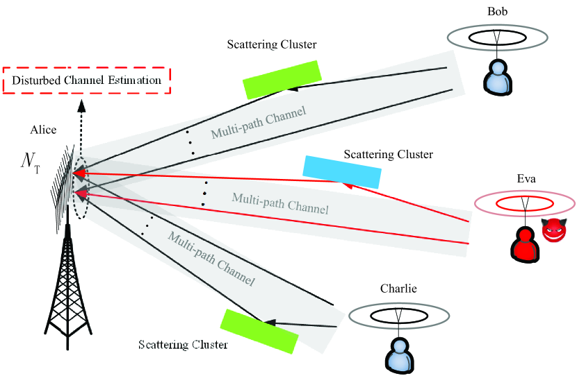
Figure 1: Uplink two-user OFDM system model under pilot spoofing attack.

Let us first turn to the representation of signal model. At each transmit (receive) antenna of nodes, the conventional OFDM modulator (demodulator) is equipped to map bit streams into frequency-domain signals transmitted on $N$ subcarriers. OFDM symbols transmitted from Bob, Charlie and Eva at time index $k$ are denoted by vectors ${{\bf{x}}_{{j}}}\left[k\right]\in{{\mathbb{C}}^{N\times 1}},j\in\left\{{{\rm{B,C,E}}}\right\}$. Those vectors are processed by inverse fast Fourier transform (IFFT) and then each added with a cyclic prefix of length $p$ to combat the multi-path influence. Generally, it is assumed that $p\geq L-1$, where $L$ is the maximum length of all channels. After removing the cyclic prefix at the $i$-th receive antenna, Alice derives the time-domain signal vector ${{\bf{y}}^{i}}\left[k\right]\in{{\mathbb{C}}^{N\times 1}}$ written as

$${{\bf{y}}^{i}}\left[k\right] = {\bf{H}}_{{\rm{C,B}}}^{i}{{\bf{F}}^{\rm{H}}}{{\bf{x}}_{\rm{B}}}\left[k\right]+{\bf{H}}_{{\rm{C,C}}}^{i}{{\bf{F}}^{\rm{H}}}{{\bf{x}}_{\rm{C}}}\left[k\right]$$ (1)

$$+ {\bf{H}}_{{\rm{C,E}}}^{i}{{\bf{F}}^{\rm{H}}}{{\bf{x}}_{\rm{E}}}\left[k\right]+{{\bf{v}}^{i}}\left[k\right]$$

where ${\bf{H}}_{{\rm{C,B}}}^{i}$, ${\bf{H}}_{{\rm{C,C}}}^{i}$ and ${\bf{H}}_{{\rm{C,E}}}^{i}$ are the $N\times N$ circulant matrices of Bob, Charlie and Eva, with the first column respectively given by ${\left[{\begin{array}[]{*{20}{c}}{{\bf{h}}_{\rm{B}}^{{i^{\rm{T}}}}}&{{{\bf{0}}_{1\times\left({N-L}\right)}}}\end{array}}\right]^{\rm{T}}}$, ${\left[{\begin{array}[]{*{20}{c}}{{\bf{h}}_{\rm{C}}^{{i^{\rm{T}}}}}&{{{\bf{0}}_{1\times\left({N-L}\right)}}}\end{array}}\right]^{\rm{T}}}$, and ${\left[{\begin{array}[]{*{20}{c}}{{\bf{h}}_{\rm{E}}^{{i^{\rm{T}}}}}&{{{\bf{0}}_{1\times\left({N-L}\right)}}}\end{array}}\right]^{\rm{T}}}$. Those $L$ by $1$ CIR vectors to the $i$-th receive antenna of Alice, i.e., ${\bf{h}}_{\rm{B}}^{i}$, ${\bf{h}}_{\rm{C}}^{i}$ and ${\bf{h}}_{\rm{E}}^{i}$, are mutually independent with each other. The channel power delay profile (PDP) of Bob, Charlie and Eva at the $j$-th path to the $i$-th antenna of Alice are respectively denoted by $\sigma_{{\rm{B}},j,i}^{2}$, $\sigma_{{\rm{C}},j,i}^{2}$, and $\sigma_{{\rm{E}},j,i}^{2}$. Without loss of generality, channel PDPs are normalized so that $\sum\limits_{j=1}^{L}{\sigma_{{l},j,i}^{2}}=1,\forall i,\forall l\in\left\{{{\rm{B,C,E}}}\right\}$ are satisfied. The CIRs of different paths exhibit spatially uncorrelated Rayleigh fading for each receiving antenna and CIRs of different antennas are assumed to be spatially correlated for each path. The receive correlation matrix of signals from Bob, Charlie and Eva are respectively denoted by ${\bf R}_{\rm B}$, ${\bf R}_{\rm C}$ and ${\bf R}_{\rm E}$. ${{\bf{v}}^{i}}\left[k\right]\in{{\mathbb{C}}^{N\times 1}}$ denotes the vector of i.i.d. random variable satisfying ${\cal C}{\cal N}\left({0,{\sigma^{2}}}\right)$ where $\sigma^{2}$ is noise power. ${\bf{F}}$ denotes the $N\times N$ unitary DFT matrix and it is easy to show that the eigenvalue decomposition of ${\bf{H}}_{{\rm{C}},j}^{i},j\in\left\{{{\rm{B,C,E}}}\right\}$ leads to ${\bf{H}}_{{\rm{C}},j}^{i}={{\bf{F}}^{\rm{H}}}{\rm{diag}}\left\{{\sqrt{N}{\bf{F}}{{\left[{\begin{array}[]{*{20}{c}}{{\bf{h}}_{{j}}^{{i^{\rm{T}}}}}&{{{\bf{0}}_{1\times\left({N-L}\right)}}}\end{array}}\right]}^{\rm{T}}}}\right\}{\bf{F}},j\in\left\{{{\rm{B,C,E}}}\right\}$. Taking FFT of received signals, Alice finally obtains the version of $N$ by $1$ frequency-domain signals ${\widetilde{\bf{y}}^{i}}\left[k\right]$ at the $i$-th receive antenna as

$${\widetilde{\bf{y}}^{i}}\left[k\right] = {\rm{diag}}\left\{{\sqrt{N}{\bf{F}}{{\left[{\begin{array}[]{*{20}{c}}{{\bf{h}}_{\rm{B}}^{{i^{\rm{T}}}}}&{{{\bf{0}}_{1\times\left({N-L}\right)}}}\end{array}}\right]}^{\rm{T}}}}\right\}{{\bf{x}}_{\rm{B}}}\left[k\right]$$ (3)

$$+ {\rm{diag}}\left\{{\sqrt{N}{\bf{F}}{{\left[{\begin{array}[]{*{20}{c}}{{\bf{h}}_{\rm{C}}^{{i^{\rm{T}}}}}&{{{\bf{0}}_{1\times\left({N-L}\right)}}}\end{array}}\right]}^{\rm{T}}}}\right\}{{\bf{x}}_{\rm{C}}}\left[k\right]$$ (5)

$$+ {\rm{diag}}\left\{{\sqrt{N}{\bf{F}}{{\left[{\begin{array}[]{*{20}{c}}{{\bf{h}}_{\rm{E}}^{{i^{\rm{T}}}}}&{{{\bf{0}}_{1\times\left({N-L}\right)}}}\end{array}}\right]}^{\rm{T}}}}\right\}{{\bf{x}}_{\rm{E}}}\left[k\right]+{{\bf{w}}^{i}}\left[k\right]$$ (7)

where ${{\bf{w}}^{i}}\left[k\right]={\bf{F}}{{\bf{v}}^{i}}\left[k\right]\in{{\mathbb{C}}^{N\times 1}}$ is the DFT projection of the random vector ${{\bf{v}}^{i}}\left[k\right]$. We see that since ${{\bf{v}}^{i}}\left[k\right]$ is isotropic, ${{\bf{w}}^{i}}\left[k\right]$ has the same distribution as ${{\bf{v}}^{i}}\left[k\right]$, i.e., a vector of i.i.d. ${\cal C}{\cal N}\left({0,{\sigma^{2}}}\right)$ random variables. After simplification, the received signal is transformed into:

$${\widetilde{\bf{y}}^{i}}\left[k\right] = {\rm{diag}}\left\{{{{\bf{x}}_{\rm{B}}}\left[k\right]}\right\}{{\bf{F}}_{\rm{L}}}{\bf{h}}_{\rm{B}}^{{i}}+{\rm{diag}}\left\{{{{\bf{x}}_{\rm{C}}}\left[k\right]}\right\}{{\bf{F}}_{\rm{L}}}{\bf{h}}_{\rm{C}}^{{i}}$$ (9)

$$+ {\rm{diag}}\left\{{{{\bf{x}}_{\rm{E}}}\left[k\right]}\right\}{{\bf{F}}_{\rm{L}}}{\bf{h}}_{\rm{E}}^{{i}}+{{\bf{w}}^{i}}\left[k\right]$$

where ${{\bf{F}}_{\rm{L}}}=\sqrt{N}{\bf{F}}\left({:,1:L}\right)$. Next, we make assumptions:

Assumption 1.

We assume ${{\bf{x}}_{\rm{B}}}\left[k\right]={x_{\rm{B}}}\left[k\right]{{\bf{1}}_{N\times 1}}$ and ${{\bf{x}}_{\rm{C}}}\left[k\right]={x_{\rm{C}}}\left[k\right]{{\bf{1}}_{N\times 1}}$ where ${{\bf{1}}_{N\times 1}}$ is a column vector whose elements are equally to be one. Alternatively, we can superimpose those pilots onto a dedicated pilot sequence optimized under a non-security oriented scenario and utilize this new pilot for training. At this point, ${{\bf{x}}_{\rm{B}}}\left[k\right]$, ${{\bf{x}}_{\rm{C}}}\left[k\right]$ can be an additional phase difference for security consideration. Signals transmitted by Eva can be denoted by ${\rm{diag}}\left\{{{{\bf{x}}_{\rm{E}}}\left[k\right]}\right\}={x_{\rm{E}}}\left[k\right]{\bf{E}}$ where ${\bf{E}}$ has dimension $N\times N$ and is unknown.

We denote the pilot tones at $k$-th symbol time by ${x_{\rm{B}}}\left[k\right],{x_{\rm{C}}}\left[k\right],{x_{\rm{E}}}\left[k\right]$ with ${x_{\rm{B}}}\left[k\right]=\sqrt{{\rho_{\rm{B}}}}{e^{j{\theta_{k}}}},{x_{\rm{C}}}\left[k\right]=\sqrt{{\rho_{\rm{C}}}}{e^{j{\beta_{k}}}},{x_{\rm{E}}}\left[k\right]=\sqrt{{\rho_{\rm{E}}}}{e^{j{\varphi_{k}}}}$ where $\rho_{\rm{B}}$, $\rho_{\rm{C}}$ and $\rho_{\rm{E}}$ respectively denote the transmitting power of Bob, Charlie and Eva.

Assumption 2.

We assume that pilot tones across adjacent symbol time are kept with fixed phase difference for each legitimate node. In this principle, we define ${\theta_{j+1}}-{\theta_{j}}=\theta,j\geq 0$, ${\beta_{j+1}}-{\beta_{j}}=\beta,j\geq 0$ where ${\theta}$, ${\beta}$ are fixed and known by all parties.

Assumption 3.

Alice can acquire ${\bf R}_{\rm B}$ and ${\bf R}_{\rm C}$ perfectly except ${\bf R}_{\rm E}$. As a basic system configuration, at least four OFDM symbols are assumed to be within one coherence time.

III-C Channel Estimation Model Under Spoofed Pilots

Now let us turn to describe the estimation models of FS channels. We note that Eq. (9) is transformed into:

$${\widetilde{\bf{y}}^{i}}\left[k\right]={{\bf{F}}_{\rm{L}}}{\bf{h}}_{\rm{B}}^{{i}}{x_{\rm{B}}}\left[k\right]+{{\bf{F}}_{\rm{L}}}{\bf{h}}_{\rm{C}}^{{i}}{x_{\rm{C}}}\left[k\right]+{\bf{E}}{{\bf{F}}_{\rm{L}}}{\bf{h}}_{\rm{E}}^{{i}}{x_{\rm{E}}}\left[k\right]+{{\bf{w}}^{i}}\left[k\right]$$ (10)

The spoofing pilots make ${\bf{E}}$ an identity matrix. Stacking the received signals across $N_{\rm T}$ antennas, Alice obtains the received signals as:

$${\bf{y}}\left[k\right]={x_{\rm{B}}}\left[k\right]{{\bf{h}}_{\rm{B}}}+{x_{\rm{C}}}\left[k\right]{{\bf{h}}_{\rm{C}}}+{x_{\rm{E}}}\left[k\right]{{\bf{h}}_{\rm{E}}}+{\bf{w}}\left[k\right]$$ (11)

Here, we have ${\bf{y}}\left[k\right]=\left[{\begin{array}[]{*{20}{c}}{{\widetilde{{\bf{y}}}^{{1^{\rm{T}}}}}\left[k\right]}&{,\ldots,}&{{\widetilde{{\bf{y}}}^{{N_{\rm{T}}}^{\rm{T}}}}\left[k\right]}\end{array}}\right]\in{{\mathbb{C}}^{1\times NN_{\rm T}}}$, ${{\bf{h}}_{{j}}}=\left[{\begin{array}[]{*{20}{c}}{{{\left({{{\bf{F}}_{\rm{L}}}{\bf{h}}_{{j}}^{1}}\right)}^{\rm{T}}}}&{,\ldots,}&{{{\left({{{\bf{F}}_{\rm{L}}}{\bf{h}}_{{j}}^{{N_{\rm{T}}}}}\right)}^{\rm{T}}}}\end{array}}\right]\in{{\mathbb{C}}^{1\times NN_{\rm T}}}$, $j\in\left\{{{\rm{B,C,E}}}\right\}$ and there exists ${\bf{w}}\left[k\right]=\left[{\begin{array}[]{*{20}{c}}{{{\bf{w}}^{{1^{\rm{T}}}}}\left[k\right]}&{,\ldots,}&{{{\bf{w}}^{{N_{\rm{T}}}^{\rm{T}}}}\left[k\right]}\end{array}}\right]\in{{\mathbb{C}}^{1\times NN_{\rm T}}}$. Collecting signals within two OFDM symbols, i.e. ${k_{1}}$ and ${k_{2}}$, Alice can further derive

$${\widehat{\bf{Y}}}{\rm{=}}{{\bf{x}}_{\rm{B}}}{{\bf{h}}_{\rm{B}}}{\rm{+}}{{\bf{x}}_{\rm{C}}}{{\bf{h}}_{\rm{C}}}+{{\bf{x}}_{\rm{E}}}{{\bf{h}}_{\rm{E}}}+{\bf{w}}$$ (12)

where ${\widehat{\bf{Y}}}={\left[{\begin{array}[]{*{20}{c}}{{{\bf{y}}^{\rm{T}}}\left[{{k_{1}}}\right]}&{{{\bf{y}}^{\rm{T}}}\left[{{k_{2}}}\right]}\end{array}}\right]^{\rm{T}}}$, ${{\bf{x}}_{{j}}}={\left[{\begin{array}[]{*{20}{c}}{{x_{{j}}}\left[{{k_{1}}}\right]}&{{x_{{j}}}\left[{{k_{2}}}\right]}\end{array}}\right]^{\rm{T}}}$, $j\in\left\{{{\rm{B,C,E}}}\right\}$ and there exists ${\bf{w}}={\left[{\begin{array}[]{*{20}{c}}{{{\bf{w}}^{\rm{T}}}\left[{{k_{1}}}\right]}&{{{\bf{w}}^{\rm{T}}}\left[{{k_{2}}}\right]}\end{array}}\right]^{\rm{T}}}$.

We consider the configuration of orthogonal pilots, namely, ${\bf{x}}_{\rm{B}}^{+}{{\bf{x}}_{\rm{C}}}=0,{\bf{x}}_{\rm{C}}^{+}{{\bf{x}}_{\rm{B}}}=0$, to put an explicit interpretation on the security problem, that is, a least square (LS) estimation of ${{{\bf{h}}_{\rm{B}}}}$ or ${{{\bf{h}}_{\rm{C}}}}$, contaminated by ${{{\bf{h}}_{\rm{E}}}}$ with a noise bias, is given by:

$${\widehat{\bf{h}}_{{\rm{con}}}}=\left\{{\begin{array}[]{*{20}{c}}{{{\bf{h}}_{\rm{B}}}+{{\bf{h}}_{\rm{E}}}+{\bf{x}}_{\rm{B}}^{+}{\bf{w}}}&{if\,\,{{\bf{x}}_{\rm{E}}}={{\bf{x}}_{\rm{B}}}}\\ {{{\bf{h}}_{\rm{C}}}+{{\bf{h}}_{\rm{E}}}+{\bf{x}}_{\rm{C}}^{+}{\bf{w}}}&{if\,\,{{\bf{x}}_{\rm{E}}}={{\bf{x}}_{\rm{C}}}}\end{array}}\right.$$ (13)

Basically, employing any nonorthogonal pilots causes the similar phenomenon. Therefore, the estimate value depends on which pilot is spoofed by Eva.

Problem 1.

Alice cannot distinguish which legitimate user is being spoofed since any prior information of the attack decision made by Eva is unavailable at Alice.

Obviously, only one spoofer can completely paralyze the whole channel estimation process for multiple users.

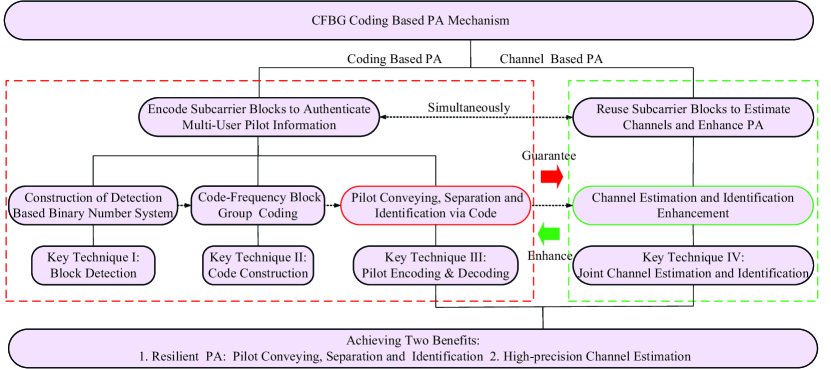
Figure 2: Methodology for CFBG coding based PA, including coding based PA and channel based PA. Particularly, coding based PA provides the basis of channel based PA which enhances coding based PA as well. The overall process embraces two key ideas and four vital implementing techniques. The ultimate result is to achieve resilient PA and high-precision channel estimation simultaneously.

Remark 1.

For single user scenario, Alice is only required to avoid pilot spoofing attack. However, in this two-user scenario, significant difference lies in the fact that Alice has to additionally guarantee the PA between legitimate nodes. Basically, Alice has to first guarantee the PA between legitimate nodes, i.e., Bob and Charlie under the circumstance of random pilots, and then avoid the Problem 1. In fact, the random pilots incur huge difficulties for PA between Bob and Charlie and this issue becomes more challenging under hybrid attack

III-D Novel Attack Environment and One Critical Challenge

Pilot randomization usually serves as a prerequisite for efficiently paralyzing the pilot spoofing attack. The commonsense is that Bob and Charlie independently randomize their own pilot tones [12, 16]. In practice, the randomization of pilot tone values is employed for CIR estimation. Theoretically, the probability of being spoofed is zero in this case.

However, those pilot tones of continuous values, when utilized for PA, have to be quantized into discrete values in a limited alphabet with high resolution, for convenience of sharing between transceiver [16]. More specifically, each of candidate pilot phases for CIR estimation is mapped into a unique quantized sample, chosen from the set ${\cal A}$ defined by ${\cal A}=\left\{{{e^{j{\theta}}}:{\theta}\sim U\left[{0,2\pi}\right)}\right\}$ where $U$ denotes the uniform distribution. This can be achieved by multiplying the traditional OFDM pilot tones with suitable sequences ${\delta_{\rm{B}}}\left[k\right]$ and ${\delta_{\rm{C}}}\left[k\right]$.

Anyway, the pilots utilized for estimation are continuous for avoiding attack while those utilized for PA must be discrete, influenced by the quantization precision. The limited-alphabet representation of pilot tones brings PA a novel problem:

Problem 2.

Eva imitates to select random pilot phases ${\varphi}$ satisfying ${\varphi_{j+1}}-{\varphi_{j}}=\varphi,j\geq 0$ from $\cal A$ and launches a spoofing attack, denoted by randomly-imitating attack. Moreover, Eva that is inspired to keep silent is also able to cheat Bob and Charlie to adopt random pilots, without costing any extra resource. This is denoted by a silence cheating mode. What’s worse, Eva can also launch pilot jamming attack with arbitrary jamming signals, in a stealthy way under the “shield” of the enjoinment of pilot randomization . Basically, Eva can launch a hybrid attack, that is, combination of randomly-imitating attack, silence cheating, and pilot jamming attack. Those behaviors are generally unpredictable.

Besides this, pilot randomization imposes on PA complex interference caused by user randomness and independence. Under this circumstance, the randomized pilot information is non-recoverable and thus the secure delivery of pilot information is challenging in the following sense:

Problem 3.

Those randomized and independent pilots, if utilized for authentication through multiuser channels, will be hidden in the random channel environment and cannot be separated, let alone identified.

IV Framework of Code-Frequency Block Group Coding Based Pilot Authentication

In this section, we identify the key points required for the design of secure PA. We develop a CFBG coding based PA framework in Fig. 2 with the following general description for its core components. .

IV-A Core of PA under Hybrid Attack

Naturally, rethinking Problem 3 inspires us to redesign the overall PA process as pilot conveying, separation and identification. Correspondingly, we have to answer three questions, including 1) How to correctly convey randomized pilots of any legitimate node to Alice? 2) How to separate multiple pilots hidden in the wireless environment with high precision? 3) how to then reliably identify those separated pilot? To answer the questions mentioned above, we identify the coding based PA in the following way:

Fact 1.

Perform pilot conveying on code domain through a codebook medium with the potential for excellent abilities of pilot separation and identification under hybrid attack.

IV-B CFBG Coding Based PA

For this concept, we stress that the advantages of information coding and channel characteristic are exploited jointly. Subcarrier blocks are reused by randomized pilots for channel estimation and simultaneously encoded for resilient PA. Generally, this process includes a coding based PA and a channel based PA. The relationship between the two methods is shown in Fig. 2, embracing four steps.

IV-B1 Step I: Construction of Detection Based Binary Number System

Basically, in order to find the desirable codebook, we need to acquire efficient features that are easy to encode and decode. A fact is that the activation patterns of subcarrier blocks of given certain size can be represented by digit 1or 0, depending on whether those subcarriers are activated or not. Hinted by this, our goal in this part is to determine the block size, precisely detect the activation patterns of each subcarrier block, and finally encode the results into binary digits. To achieve this, a block detection technique is proposed and detailed in Section V. In this way, assuming the whole subcarriers are divided and grouped into $B$ blocks each of which has ${{{N}}\mathord{\left/{\vphantom{{{N}}B}}\right.\kern-1.2pt}B}$ subcarriers, we can define a set of binary code vector as ${\cal S}=\left\{{\left.{\bf{s}}\right|{s_{i}}\in\left\{{0,1}\right\},1\leq i\leq{L_{s}}}\right\}$ where ${L_{s}}$ denotes the maximum length of the code.

IV-B2 Step II: Code-Frequency Block Group Coding

In order to formulate the codebook medium required, we first construct a code frequency domain on the basis of the binary number system. It is constituted by a set of pairs $\left({{\bf{c}},b}\right)$ in Fig. 3(a), where ${\bf{c}}\in\cal S$ and $b,1\leq b\leq B$ is an integer which represents the subcarrier block index of appearance of the code. $B$ is the maximum number of available blocks supported. In what follows, by grouping and scheduling multiple binary digits on code-frequency domain, we have the potential for formulating a codebook, for example, with the dimension of $B$ by $C$ if patterns of total number $C$ are supported. The key requirement is developing a suitable coding method such that a mapping from a codeword to the activation patterns is formulated and unique patterns can be created extensively. Further optimizing the code, we could construct the codebook achieving Fact 1 by a technique of CFBG coding which is detailed in Section VI.

IV-B3 Step III: Pilot Conveying, Separation and Identification via Code

Based on the theoretical codebook, we turn to the practical construction of conveying, separation and identification of pilot phase information. At this point, pilot conveying means encoding pilot phases into activation patterns through the codebook. Pilot separation and identification functions to achieve resilient decoding of phase information from the observed patterns, disturbed under multi-user codeword interference and hybrid attack. An implementation of the overall process in two-user OFDM systems is indicated in Fig. 3(b), including three components, i.e., a Block Identity (ID) Mapper, a Block Creator, a Detector and a Identifer. The key is the proposed pilot encoding and decoding technique which is further detailed in Section VII.

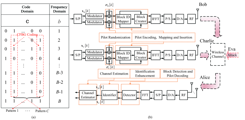
Figure 3: Theoretical support and practical implementation for CFBG coding based PA mechanism; (a) General description of CFBG coding theory on code-frequency domain; (b) Implementation framework of CFBG coding based PA mechanism for a two-user uplink OFDM systems.

IV-B4 Step IV: Channel Estimation and Identification Enhancement

On the basis of coding based PA, identified pilots are utilized for channel estimation. Channel based PA is performed at an Estimator. The principle is that the spatial correlation property of estimated channels are employed for enhancing pilot identification. The detailed technique is shown in Section VIII. In the following sections, we will extend the four key techniques in details.

V Key Technique I: Block Detection

In this section, we present how to exploit signal detection technique to execute the step I.

V-A Construction of 4-Hypotheses Testing

Observing the possible number $i$ of signals coexisting on one block, we can respectively define the hypotheses by ${{\cal H}_{i}},i=0,1,2,3$ under which the received signals stacked in four OFDM symbols, can be represented by

$${\bf{Y}}={\bf{DH}}+{\bf{W}}$$ (14)

Here, we have ${\bf{Y}}={\left[{{{\bf{y}}^{\rm{T}}}{{\left[{{k_{i}}}\right]}_{0\leq i\leq 3}}}\right]^{\rm{T}}}\in{{\mathbb{C}}^{4\times NN_{\rm T}}}$, and ${\bf{W}}={\left[{{{\bf{w}}^{\rm{T}}}{{\left[{{k_{i}}}\right]}_{0\leq i\leq 3}}}\right]^{\rm{T}}}\in{{\mathbb{C}}^{4\times NN_{\rm T}}}$. The components of ${\bf{H}}\in{{\mathbb{C}}^{i\times NN_{\rm T}}}$ and ${\bf{D}}\in{{\mathbb{C}}^{4\times i}}$ are selected from ${\bf{h}}_{j}$ and ${\bf{x}}_{j}$, $j\in\left\{{{\rm{B,C,E}}}\right\}$, depending on the specific nodes coexisting on one block. Note that additive vector ${\bf{W}}$ is independent of channel vectors ${\bf{H}}$. We define the covariance matrix by ${\bf{R}}=\frac{1}{{{N_{\rm{T}}}N}}{\bf{Y}}{{\bf{Y}}^{\rm{H}}}$. According to the law of large number (LLN), the following equation can be satisfied:

$${\bf{R}}\xlongrightarrow[{N_{\rm{T}}}N\to\infty]{\rm{a.s.}}\frac{1}{{{N_{\rm{T}}}N}}{{\rm{\mathbb{E}}}_{\bf{H}}}\left\{{{\bf{DH}}{{\bf{H}}^{\rm{H}}}{{\bf{D}}^{\rm{H}}}}\right\}{\rm{+}}\frac{1}{{{N_{T}}N}}{{\rm{\mathbb{E}}}_{\bf{W}}}\left\{{{\bf{W}}{{\bf{W}}^{\rm{H}}}}\right\}$$ (15)

Examining the equation, we know that the rank of first term is equal to $i$ under ${{\cal H}_{i}},i=0,1,2,3$ and the rank of second term is always four. Under the hypothesis of ${{\cal H}_{1}}$, the eigenvalues of ${\bf{R}}$ with the exception of the largest one can all be approximately equal to the noise variance ${\sigma^{2}}$. The approximation becomes exact as ${N_{\rm{T}}}N\to\infty$. Therefore, it is possible to infer the absence or presence of the signals by comparing the largest eigenvalue with the smallest one. Similarly, the existence of $i$-th signals $2\leq i\leq 3$, under the hypothesis of ${{\cal H}_{i}}$, depends on the comparison of the $i$-th largest eigenvalue with the smallest one.

 

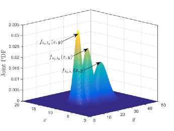
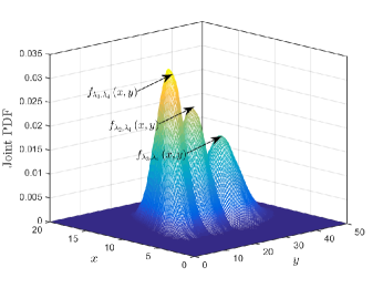
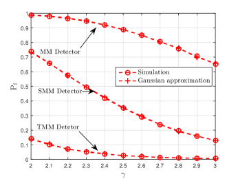
   (a)                                                (b)                                                (c)

Figure 4: Simulations of joint-PDF approximation and detection performance; (a) Analytical joint PDFs under $NN_{\rm T}=20$ (based on approximation approach with ${\rho_{1}}=0.16$, ${\rho_{2}}=0.26$, ${\rho_{3}}=0.43$); (b) Simulated joint PDFs under $NN_{\rm T}=20$ (based on empirical approach); (c) PF versus $\gamma$ under ${\rho_{1}}=0.16$, ${\rho_{2}}=0.26$, ${\rho_{3}}=0.43$, and $N_{\rm T}N=20$.

V-B Ordered Signal Detection

Three detectors are required to detect the possible number of signals on each block. In the descending order of eigenvalue values, we denote the predesigned detectors respectively by (Maximum-Minimum ) MM detector, (Second-Maximum-Minimum) SMM detector, (Third-Maximum-Minimum) TMM detector. We formulate the normalized covariance matrix as $\widehat{\bf{R}}=\frac{1}{{{\sigma^{2}}}}{\bf{Y}}{{\bf{Y}}^{\rm{H}}}\in{{\mathbb{C}}^{4\times 4}}$ and suppose that the ordered eigenvalue of $\widehat{\bf{R}}$ are ${\lambda_{1}}>{\lambda_{2}}>{\lambda_{3}}>{\lambda_{4}}>0$. The test statistics are therefore respectively denoted by

$$T_{\rm MM}=\frac{{{\lambda_{1}}}}{{{\lambda_{4}}}},T_{\rm SMM}=\frac{{{\lambda_{2}}}}{{{\lambda_{4}}}},T_{\rm TMM}=\frac{{{\lambda_{3}}}}{{{\lambda_{4}}}}$$ (16)

A unified decision threshold, denoted by $\gamma$, is configured using

$$T_{\rm MM}\mathop{\gtrless}\limits_{{{{\cal H}_{0}}}}^{{{{\cal H}_{1}}}}\gamma,T_{\rm SMM}\mathop{\gtrless}\limits_{{{{{\overline{\cal H}}_{2}}}}}^{{{{\cal H}_{2}}}}\gamma,T_{\rm TMM}\mathop{\gtrless}\limits_{{{{{\overline{\cal H}}_{3}}}}}^{{{{\cal H}_{3}}}}\gamma$$ (17)

where ${{\overline{\cal H}}_{2}}$ and ${{\overline{\cal H}}_{3}}$ represent two alternative hypotheses that are respectively contrary to the hypothesis ${{{\cal H}}_{2}}$ and ${{{\cal H}}_{3}}$. Therefore, identifying the exact number of signals on one block can be achieved by an ordered detection and decision for composite hypotheses. For example, the existence of only one signal is equivalent to successfully verifying ${{\overline{\cal H}}_{3}}$, then ${{\overline{\cal H}}_{2}}$ and finally ${{{\cal H}}_{1}}$. Generally, the testing performance is measured by the probability of detection (PD) and the probability of false alarm (PF) which are respectively denoted for each detector by

$$\begin{array}[]{l}{\rm{P}}_{\rm{D}}^{{\rm{MM}}}={\rm{Pr}}\left({\left.{{H_{1}}}\right|{H_{1}}}\right),{\rm{P}}_{\rm{F}}^{{\rm{MM}}}={\rm{Pr}}\left({\left.{{H_{1}}}\right|{H_{0}}}\right)\\ {\rm{P}}_{\rm{D}}^{{\rm{SMM}}}={\rm{Pr}}\left({\left.{{H_{\rm{2}}}}\right|{H_{\rm{2}}}}\right),{\rm{P}}_{\rm{F}}^{{\rm{SMM}}}={\rm{Pr}}\left({\left.{{H_{\rm{2}}}}\right|{{{\overline{\cal H}}_{2}}}}\right)\\ {\rm{P}}_{\rm{D}}^{{\rm{TMM}}}={\rm{Pr}}\left({\left.{{H_{\rm{3}}}}\right|{H_{\rm{3}}}}\right),{\rm{P}}_{\rm{F}}^{{\rm{TMM}}}={\rm{Pr}}\left({\left.{{H_{\rm{3}}}}\right|{{{\overline{\cal H}}_{3}}}}\right)\end{array}$$ (18)

Remark 2.

The number of signals coexisting on one subcarrier block is not deterministic due to the random activation patterns and cannot be predicted in advance. Therefore, the common decision threshold $\gamma$ could guarantee that the number of signals could be always precisely detected using a single threshold. Furthermore, this setup ensures an analytical expression of $\gamma$ in the following.

V-C Determination of $\gamma$

Examing Eq. (10), we stress that the first step is to determine the joint moments of two arbitrary eigenvalues. Then we derive the closed-form decision threshold $\gamma$ based on the probability density function (PDF) approximated from those moments.

V-C1 Determination of Moments

Considering $\widehat{\bf{R}}$ under hypotheses ${{{\cal H}}_{0}}$, we find that the joint distribution of first eigenvalue and smallest one is equivalent to that of a Wishart matrix satisfying ${\cal C}{\cal W}\left({{N_{T}}N,{{\bf{I}}_{4}}}\right)$ [29]. Under ${{\overline{\cal H}}_{i}}$ for $2\leq i\leq 3$, the joint distribution of $i$-th eigenvalue with smallest one is equivalent to that of the Wishart matrix. Finally, a closed expression of joint moments of $\lambda_{i}$ and $\lambda_{j}$ is calculated by:

$${\mathbb{E}}\left({\lambda_{i}^{m}\lambda_{j}^{n}}\right)=\sum\limits_{\left\{{a,b,c,d}\right\}\subseteq\left\{{{A_{1}}\cup{A_{2}}}\right\}}{K{B_{a,b,c,d}}{f_{i,j,m,n}}\left({a,b,c,d}\right)}$$ (19)

where

$$\left\{{i,j,m,n}\right\}\subseteq\left\{\begin{array}[]{l}\left\{{1,4,1,1}\right\},\left\{{1,4,m,0}\right\},\left\{{1,4,0,n}\right\},\\ \left\{{2,4,1,1}\right\},\left\{{2,4,m,0}\right\},\left\{{3,4,1,1}\right\},\\ \left\{{3,4,m,0}\right\},1\leq m,n\leq 2\end{array}\right\}$$ (23)

Here there exist ${{\cal A}_{1}}{\rm{=}}\left\{{\left\{{a,b,c,d}\right\}\left|{\left\{{a,b,c,d}\right\}\subseteq\left\{{0\cup{{\cal B}_{1}}}\right\}}\right.}\right\}$, and ${{\cal A}_{2}}{\rm{=}}\left\{{\left\{{a,b,c,d}\right\}\left|{\left\{{a,b,c,d}\right\}\subseteq}\right.{{\cal B}_{2}}}\right\}$. For ${{\cal B}_{1}}$ and ${{\cal B}_{2}}$,

$${{\cal B}_{1}}{\rm{=}}\left\{{{{\cal S}_{\left\{{2,4,6}\right\}}},{{\cal S}_{\left\{{2,5,5}\right\}}},{{\cal S}_{\left\{{3,3,6}\right\}}},{{\cal S}_{\left\{{3,4,5}\right\}}},{{\cal S}_{\left\{{4,4,4}\right\}}}}\right\}$$ (24)

$${{\cal B}_{2}}{\rm{=}}\left\{\begin{array}[]{l}{{\cal S}_{\left\{{1,1,4,6}\right\}}},{{\cal S}_{\left\{{1,1,5,5}\right\}}},{{\cal S}_{\left\{{1,2,3,6}\right\}}},{{\cal S}_{\left\{{1,3,3,5}\right\}}},\\ {{\cal S}_{\left\{{1,2,4,5}\right\}}},{{\cal S}_{\left\{{1,3,4,4}\right\}}},{{\cal S}_{\left\{{2,2,2,6}\right\}}},{{\cal S}_{\left\{{2,2,3,5}\right\}}},\\ {{\cal S}_{\left\{{2,2,4,4}\right\}}},{{\cal S}_{\left\{{2,3,3,4}\right\}}},{{\cal S}_{\left\{{3,3,3,3}\right\}}}\end{array}\right\}$$ (28)

where ${{\cal S}_{\left\{{\cdot}\right\}}}$ represents the permutation of the elements of set.

$${f_{2,4,m,0}}\left({a,b,c,d}\right) = \sum\limits_{{k_{1}}=0}^{N+a-4}{\frac{{{K_{2}}\left({{{\overline{k}}_{1}}+{k_{1}}+m}\right)!{{\overline{k}}_{1}}!}}{{{k_{1}}!{2^{{{\overline{k}}_{2}}+{k_{1}}+m+1}}}}}-\sum\limits_{{k_{1}}=0}^{N+a-4}{\sum\limits_{{k_{2}}=0}^{{{\overline{k}}_{2}}}{\frac{{{K_{2}}\left({{{\overline{k}}_{2}}+{k_{1}}+{k_{2}}+m}\right)!{{\overline{k}}_{1}}!}}{{{k_{1}}!{k_{2}}!{3^{{{\overline{k}}_{2}}+{k_{1}}+{k_{2}}+m+1}}}}}}$$

$$- \sum\limits_{{k_{1}}=0}^{N+a-4}{\sum\limits_{{k_{2}}=0}^{N+d-4}{\frac{{{K_{2}}\left({{{\overline{k}}_{2}}+{k_{1}}+m}\right)!\left({{{\overline{k}}_{1}}+{k_{2}}}\right)!}}{{{k_{1}}!{k_{2}}!{2^{{{\overline{k}}_{1}}+{k_{2}}+1}}{2^{{{\overline{k}}_{2}}+{k_{1}}+m+1}}}}}}+\sum\limits_{{k_{1}}=0}^{N+a-4}{\sum\limits_{{k_{2}}=0}^{N+d-4}{\sum\limits_{{k_{3}}=0}^{{{\overline{k}}_{2}}+{k_{2}}}{\frac{{{K_{2}}\left({{{\overline{k}}_{1}}+{k_{2}}}\right)!\left({{{\overline{k}}_{2}}+{k_{1}}+{k_{3}}+m}\right)!}}{{{k_{1}}!{k_{2}}!{k_{3}}!{2^{{{\overline{k}}_{2}}+{k_{\rm{2}}}-{k_{\rm{3}}}+1}}{4^{{{\overline{k}}_{2}}+{k_{1}}+{k_{3}}+m+1}}}}}}}$$

$${f_{3,4,m,0}}\left({a,b,c,d}\right)=\sum\limits_{{k_{1}}=0}^{N+a-4}{\sum\limits_{{k_{2}}=0}^{{{\overline{k}}_{2}}+{k_{1}}}{\frac{{{K_{2}}\left({{{\overline{k}}_{1}}+{k_{2}}+m}\right)!\left({{{\overline{k}}_{2}}+{k_{1}}}\right)!}}{{{k_{1}}!{k_{2}}!{2^{{{\overline{k}}_{2}}+{k_{1}}-{k_{2}}+1}}{3^{{{\overline{k}}_{1}}+{k_{2}}+m+1}}}}}}-\sum\limits_{{k_{1}}=0}^{N+a-4}{\sum\limits_{{k_{2}}=0}^{{{\overline{k}}_{2}}+{k_{1}}}{\sum\limits_{{k_{3}}=0}^{N+d-4}{\frac{{{K_{2}}\left({{{\overline{k}}_{1}}+{k_{2}}+{k_{3}}+m}\right)!\left({{{\overline{k}}_{2}}+{k_{1}}}\right)!}}{{{k_{1}}!{k_{2}}!{k_{3}}!{2^{{{\overline{k}}_{2}}+{k_{1}}-{k_{2}}+1}}{4^{{{\overline{k}}_{1}}+{k_{2}}+{k_{3}}+m+1}}}}}}}$$ (18)

$${f_{2,4,1,1}}\left({a,b,c,d}\right) = \sum\limits_{{k_{1}}=0}^{{{\overline{k}}_{3}}-m}{\sum\limits_{{k_{2}}=0}^{{{\overline{k}}_{1}}}{\sum\limits_{{k_{3}}=0}^{{k_{1}}+{{\overline{k}}_{2}}+m}{\frac{{\left({{{\overline{k}}_{3}}-m}\right)!\left({{k_{1}}+{{\overline{k}}_{2}}+m}\right)!{{\overline{k}}_{3}}!\left({{k_{4}}-{k_{1}}-1}\right)!}}{{{k_{1}}!{k_{2}}!{k_{3}}!{2^{N+b+{k_{\rm{1}}}-{k_{\rm{3}}}+m-3}}{4^{N+d+{k_{2}}+{k_{3}}+m-3}}}}}}}$$ (19)

$$- \sum\limits_{{k_{1}}=0}^{{{\overline{k}}_{3}}-m}{\sum\limits_{{k_{2}}=0}^{{{\overline{k}}_{1}}}{\sum\limits_{{k_{3}}=0}^{{{\overline{k}}_{2}}+{k_{1}}+{k_{2}}+m}{\frac{{\left({{{\overline{k}}_{3}}-m}\right)!\left({{k_{1}}+{{\overline{k}}_{2}}+{k_{2}}+m}\right)!{{\overline{k}}_{1}}!\left({{k_{4}}-{k_{1}}-{k_{2}}-1}\right)!}}{{{k_{1}}!{k_{2}}!{k_{3}}!{3^{N+b+{k_{\rm{1}}}+{k_{2}}-{k_{3}}+m-3}}{4^{N+d+{k_{3}}+m-3}}}}}}}$$

$${f_{3,4,1,1}}\left({a,b,c,d}\right)=\sum\limits_{{k_{1}}=0}^{{{\overline{k}}_{3}}-m}{\sum\limits_{{k_{2}}=0}^{{{\overline{k}}_{2}}+{k_{1}}}{\sum\limits_{{k_{3}}=0}^{{{\overline{k}}_{1}}+{k_{2}}+m}{\frac{{\left({{{\overline{k}}_{3}}-m}\right)!\left({{{\overline{k}}_{2}}+{k_{1}}}\right)!\left({{{\overline{k}}_{1}}+m+{k_{2}}}\right)!\left({{k_{4}}-{k_{1}}-{k_{2}}-1}\right)!}}{{{k_{1}}!{k_{2}}!{k_{3}}!{2^{{{\overline{k}}_{2}}+{k_{\rm{1}}}-{k_{2}}+1}}{3^{{{\overline{k}}_{1}}+{k_{2}}-{k_{3}}+m+1}}{4^{{k_{4}}-{k_{1}}-{k_{2}}}}}}}}}$$ (20)

$${{B}_{a,b,c,d}}=\left\{{\begin{array}[]{*{20}{c}}{-6}&{\left\{{a,b,c,d}\right\}\subseteq\left\{{{{\cal S}_{\left\{{0,4,4,4}\right\}}}\cup{{\cal S}_{\left\{{2,3,3,4}\right\}}}}\right\}}\\ {-4}&{\left\{{a,b,c,d}\right\}\subseteq{{\cal S}_{\left\{{1,3,3,5}\right\}}}}\\ 1&{\left\{{a,b,c,d}\right\}\subseteq{{\cal S}_{\left\{{0,2,4,6}\right\}}}}\\ 2&{\left\{{a,b,c,d}\right\}\subseteq\left\{{{{\cal S}_{\left\{{0,3,4,5}\right\}}}\cup{{\cal S}_{\left\{{1,2,3,6}\right\}}}}\right\}}\\ 4&{\left\{{a,b,c,d}\right\}\subseteq\left\{{{{\cal S}_{\left\{{1,1,5,5}\right\}}}\cup{{\cal S}_{\left\{{1,3,4,4}\right\}}}\cup{{\cal S}_{\left\{{2,2,3,5}\right\}}}\cup{{\cal S}_{\left\{{2,2,4,4}\right\}}}}\right\}}\\ {24}&{\left\{{a,b,c,d}\right\}\subseteq{{\cal S}_{\left\{{3,3,3,3}\right\}}}}\\ {-2}&{\rm otherwise}\end{array}}\right.$$ (21)

The specific function $f$ can be shown from Eq. (V-C1) to Eq. (20) where ${\overline{k}_{1}}=N{N_{\rm{T}}}+c-4$, ${\overline{k}_{2}}=N{N_{\rm{T}}}+b-4$, ${\overline{k}_{3}}=N{N_{\rm{T}}}+a+m-4$, ${k_{4}}=N{N_{\rm{T}}}+d+{k_{1}}+{k_{2}}+{k_{3}}+m-3$ and ${K_{2}}=\Gamma\left({N{N_{\rm{T}}}+a-3}\right)\Gamma\left({N{N_{\rm{T}}}+d-3}\right)$. $\Gamma\left(\cdot\right)$ is the Gamma function. Note that the other function ${f_{1,4,1,1}}\left({a,b,c,d}\right)$, ${f_{1,4,0,n}}\left({a,b,c,d}\right)$ and ${f_{1,4,m,0}}\left({a,b,c,d}\right)$ can be found in [30]. $K$ satisfies $K=\frac{1}{{12\left({{N{N_{\rm{T}}}}-1}\right)!\left({{N{N_{\rm{T}}}}-2}\right)!\left({{N{N_{\rm{T}}}}-3}\right)!\left({{N{N_{\rm{T}}}}-4}\right)!}}$ and ${{B}_{a,b,c,d}}$ is shown in Eq. (21).

V-C2 Analytical Solution of $\gamma$

Inspired from the method in [30], we consider the joint PDF of any eigenvalue (except the smallest one) and the smallest one can be approximated similarly, that is, for $1\leq i\leq 3$,

$${f_{{\lambda_{i}},{\lambda_{4}}}}\left({x,y}\right)=\frac{1}{{2\pi{\xi_{{\lambda_{i}}}}{\xi_{{\lambda_{4}}}}\sqrt{1-{\rho_{i}^{2}}}}}\exp\left\{{-\frac{\kappa_{i}}{{2{{\left({1-\rho_{i}}\right)}^{2}}}}}\right\}$$ (22)

where ${\xi_{{\lambda_{i}}}}$ denote the standard deviation of the eigenvalue ${{\lambda_{i}}}$ and can be derived in Eq. (19). $\rho_{i}$ is the correlation coefficient between $\lambda_{i}$ and ${\lambda_{4}}$. The parameter $\rho_{i}$ is given by $\rho_{i}=\frac{{{\zeta_{{\lambda_{i}},{\lambda_{4}}}}-{\zeta_{{\lambda_{i}}}}{\zeta_{{\lambda_{4}}}}}}{{{\xi_{{\lambda_{i}}}}{\xi_{{\lambda_{4}}}}}},1\leq i\leq 3$ and $\kappa_{i}$ is extended as:

$$\kappa_{i}=\frac{{{{\left({x-{\zeta_{{\lambda_{i}}}}}\right)}^{2}}{\rm{+}}2\rho_{i}{\xi_{{\lambda_{i}}}}{\xi_{{\lambda_{4}}}}\left({x-{\zeta_{{\lambda_{i}}}}}\right)\left({y-{\zeta_{{\lambda_{4}}}}}\right){\rm{+}}{{\left({y-{\zeta_{{\lambda_{4}}}}}\right)}^{2}}}}{{\xi_{{\lambda_{i}}}^{2}\xi_{{\lambda_{4}}}^{2}}}$$ (23)

where ${\zeta_{{\lambda_{i}}}}$ denote the expectation of ${\lambda_{i}}$ and ${\zeta_{{\lambda_{i}},{\lambda_{4}}}}$ represent the expectation of two-variate variable ${\lambda_{i}}$ and ${\lambda_{4}}$.

More accurately, we compare the joint PDF generation using the approximation approach with that using the empirical approach by simulations under $NN_{\rm T}=20$. Specifically, Fig. 4(a) illustrates the one using approximation approach whereas Fig. 4(b) shows the one based on the empirical approach. We can see that the PDFs under two methods are almost in agreement provided that the mean and the variance of the eigenvalues and correlation between them can be obtained.

Based on the approximated PDFs and given threshold $\gamma_{i}$, the cumulative distribution function (CDF) of the ratio between ${\lambda_{i}}$ and ${\lambda_{4}}$, denoted by $F_{i}\left(\gamma_{i}\right)$, can be expressed by $F_{i}\left(\gamma_{i}\right)=\Phi\left\{{\frac{{{\zeta_{{\lambda_{4}}}}\gamma_{i}-{\zeta_{{\lambda_{i}}}}}}{{{\xi_{{\lambda_{i}}}}{\xi_{{\lambda_{4}}}}\chi\left(\gamma_{i}\right)}}}\right\},\chi\left(\gamma_{i}\right)=\sqrt{\frac{{{\gamma_{i}^{2}}}}{{\xi_{{\lambda_{i}}}^{2}}}-\frac{{2\rho_{i}\gamma_{i}}}{{{\xi_{{\lambda_{i}}}}{\xi_{{\lambda_{4}}}}}}+\frac{1}{{\xi_{{\lambda_{4}}}^{2}}}}$. Here $\Phi\left\{\cdot\right\}$ denotes CDF of a standard Gaussian random variable. We then can determine ${\gamma_{i}}$ by $\gamma_{i}\buildrel\Delta\over{=}f_{i}\left({N{N_{\rm{T}}}}\right)=\frac{{{\zeta_{{\lambda_{i}}}}{\zeta_{{\lambda_{4}}}}-\tau_{i}^{2}{\rho_{i}}{\xi_{{\lambda_{i}}}}{\xi_{{\lambda_{4}}}}+{\tau_{i}}\sqrt{{\delta_{i}}-2{\rho_{i}}{\xi_{{\lambda_{i}}}}{\xi_{{\lambda_{4}}}}{\zeta_{{\lambda_{i}}}}{\zeta_{{\lambda_{4}}}}}}}{{\zeta_{{\lambda_{4}}}^{2}-\tau_{i}^{2}\xi_{{\lambda_{4}}}^{2}}}$ where ${\delta_{i}}=\zeta_{{\lambda_{i}}}^{2}\xi_{{\lambda_{4}}}^{2}+\zeta_{{\lambda_{4}}}^{2}\xi_{{\lambda_{i}}}^{2}+\left({\rho_{i}^{2}-1}\right)\tau_{i}^{2}\xi_{{\lambda_{i}}}^{2}\xi_{{\lambda_{4}}}^{2}$, $\tau_{i}={\Phi^{-1}}\left\{F_{i}\left(\gamma_{i}\right)\right\}$.

The optimal $\gamma$ should make all the expression forms of PF in Eq. (18) approach the values that are as small as possible.

Theorem 1.

Given an upper bound of PF, denoted by $P$ and with arbitrary value, the decision threshold $\gamma$ able to guarantee $1-F_{i}\left(\gamma\right)\leq P,\forall 1\leq i\leq 3$ is given by:

$$\gamma=\max\left\{{{\gamma^{*}_{1}},{\gamma^{*}_{2}},{\gamma^{*}_{3}}}\right\}$$ (24)

where ${\gamma^{*}_{i}}$ satisfies ${F_{i}}\left({{\gamma^{*}_{i}}}\right)=1-P$. And ${N{N_{\rm{T}}}}$ achieving $\gamma$ can be calculated according to:

$$N{N_{\rm{T}}}={f^{-1}_{{i_{{\rm{opt}}}}}}\left(\gamma\right)$$ (25)

where ${i_{{\rm{opt}}}}=\mathop{\arg\max}\limits_{i}{\gamma^{*}_{i}}$

The verification of this theorem is easy since ${F_{i}}$ is a monotonically-increasing function of $\gamma$. We compare the PF performance of three detectors in Fig. 4(c) where two different approaches are respectively simulated, that is, the Monte Carlo simulation and Gaussian approximation. $NN_{\rm T}$ is configured to be 20. As shown in the figure, PF curves using theoretical approximation match well with those under practical simulation. Three types of PF gradually decreases to be zero as well, with the increase of $\gamma$.

V-D Formulation of Detection Based Binary Number System

Basically, theorem 1 provides a quantitative method for measuring how many subcarriers are required in one block for precise coding with zero PF and perfect PD. Therefore, we have the following proposition:

Proposition 1.

The number $N^{*}$ of subcarriers in one subcarrier block that are enabled to precisely carry binary number information can be calculated from the Eq. (25) by configuring $P$ to be an arbitrarily small value.

Generally, when we define the total number of subcarriers allocated for channel estimation as $N_{\rm Total}$, typically equal to several hundreds, $N^{*}$ satisfies $N^{*}={{{N_{{\rm{Total}}}}}\mathord{\left/{\vphantom{{{N_{{\rm{Total}}}}}B}}\right.\kern-1.2pt}B}$.

To verify the proposition, let us turn to a 3D plot of PD and PF versus the threshold $\gamma$ and $NN_{\rm T}$ in Fig. 5(a). As we can see, with $NN_{\rm T}=60,\gamma=3$, PF is equal to zero while the PD is always maintained to be 1 for all the three detectors. In this sense, $N^{*}N_{\rm T}=60$ is enough for precise coding when $\gamma=3$. A control variable $N_{\rm B}$ is defined by

$${N_{\rm{B}}}{\buildrel\Delta\over{=}}N^{*}N_{\rm T}={{{N_{{\rm{Total}}}}{N_{\rm{T}}}}\mathord{\left/{\vphantom{{{N_{{\rm{Total}}}}{N_{\rm{T}}}}B}}\right.\kern-1.2pt}B}$$ (26)

Therefore, we know that any block configured with $N_{\rm B}\geq 60$ can carry binary number information precisely. When each block satisfies those requirements, each code digit ${c_{i}}$ that corresponds to the $i$-th subcarrier block is endowed with the following binary number:

$${c_{i}}=\left\{{\begin{array}[]{*{20}{c}}1&{if\,\,\,there\,\,\,exist\,\,\,signals}\\ 0&{otherwise}\end{array}}\right.$$ (27)

VI Key Technique II: Code Construction

On the basis of coded subcarrier blocks, we, in this section, develop a CFBG coding theory to construct a binary group code with fixed length and constant weight.

VI-A Binary Arithmetic Rule Between Codewords

The binary arithmetic rule between any two codewords to be designed is necessary and should be able to represent the overlapping operation precisely. Intuitively, two rules on the code-frequency domain can be identified and mathematically interpreted as follows:

Definition 1.

The superposition (SP) sum ${\bf{z}}={\bf{x}}{{V}}{\bf{y}}$ (designated as the digit-by-digit Boolean sum) of two $B$-dimensional binary vectors ${\bf{x}}=\left({{x_{1}},{x_{2}},\ldots,{x_{B}}}\right)$ and ${\bf{y}}=\left({{y_{1}},{y_{2}},\ldots,{y_{B}}}\right)$ is defined by:

$${z_{i}}=\left\{{\begin{array}[]{*{20}{c}}0&{if\,\,{x_{i}}={y_{i}}=0}\\ 1&{otherwise}\end{array}}\right.,\forall 1\leq i\leq{B}$$ (28)

and we say that a binary vector $\bf x$ includes a binary vector $\bf y$ if the Boolean sum satisfies ${\bf{y}}{{V}}{\bf{x}}={\bf{x}}$

Definition 2.

The algebraic superposition (ASP) sum (designated as the digit-by-digit sum) is defined by ${\bf{d}}={\bf{x}}{{V}}{\bf{y}}$ in which two $B$-dimensional binary vectors ${\bf{x}}=\left({{x_{1}},{x_{2}},\ldots,{x_{B}}}\right)$ and ${\bf{y}}=\left({{y_{1}},{y_{2}},\ldots,{y_{B}}}\right)$ satisfy:

$${{d}_{i}}={{x}_{i}}+{{y}_{i}},\forall 1\leq i\leq{B}$$ (29)

VI-B Coding Principle

Establishment of CFBG coding on the basis of the formulated binary code requires us to thoroughly analyze the issues induced by specific superposition rules. We attempt to achieve pilot conveying using binary code satisfying the principle of SP sum. In this case, several key coding principles constrained by Problem 2 can be identified.

First, we have to admit that Eva can launch randomly-imitating attack, namely, selecting randomly one codeword in the same publicly-known code as Bob (or Charlie) and activating subcarrier blocks as the codeword indicates. Therefore, we hope to guarantee that each superposition of up to three different codewords is unique and each superimposed codeword can be uniquely and correctly decomposed into original codewords. To achieve this, we propose two principles:

Principle 1.

Every sum of up to three different codewords can be decomposed by no codeword other than those used to form the sum.

Principle 2.

Every sum of up to three different codewords is distinct from every other sum of three or fewer codewords.

Remark 3.

Thanks to the sum operation for up to three different codewords, proposed CFBG method applies to single-user scenario threaten by an additional attacker Eva.

The code satisfying the two principles can be divided by two independent codes, respectively for Bob and Charlie, thus distinguishing their own codewords from each other. In this way, the silence of Eva, if exists, can be detected since any superimposition from extra codewords will induce a complete new observation codeword at Alice, therefore indicating the existence of an attack.

Randomly-imitating attack is also enabled to be detected perfectly since any extra duplicate codeword can transform original superposition codewords ( superimposed by Bob and Charlie) into a novel distinct and identifiable codeword in the code. This is determined by the two principles, which is, however, unreliable when a wideband jamming attack happens.

Problem 4.

When a wideband jamming attack happens, the interpreted codeword at Alice is a vector with all elements“1” which carry no information useful for Alice. The codewords decomposed from the superimposed codeword under the attack may also belong to the code. In this case, Alice will ignore jamming attack and make a wrong decision that there exists no attack.

To solve this issue, we reconsider the two principles and discover an important property, that is,

Property 1.

For every sum of up to three different codewords within the code, if we reduce by one any codeword digit indicating single signal on the subcarrier block, the resulted codeword can be decomposed by no codeword in the code.

This requires the previous block detection technique combined with the process of code design. We stress that this property can resolve Problem 4 and its effectiveness can be interpreted by the following fact:

Fact 2.

Under jamming attack, any superimposed digit indicating single signal on a subcarrier block logically suggests that the digits previously exploited by Bob and Charlie at the same position are both of zero value. Therefore, if we reduce those digits to be zero, the weight of interpreted codewords is unchanged. The interpreted codewords will belong to the original codebook. Otherwise when there is no jamming attack, we can know that there exist non-zero digits exploited by Bob and/or Charlie at the same digit positions and any reduction of those digits will induce the interpreted codeword of less weight as well. In this case, the interpreted codeword will never belong to the predesigned code and finally we can distinguish whether jamming attack happens.

In summary, the two principles not only guarantee the identification and classification for hybrid attack, but also provide the basic functionalities of codeword conveying, separation and identification. Obviously, those principles combined with block detection technique constitute the core of CFBG code.

 

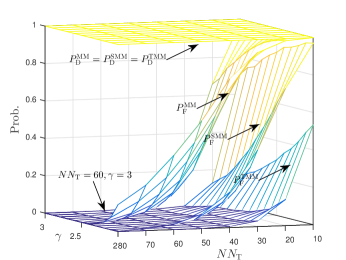
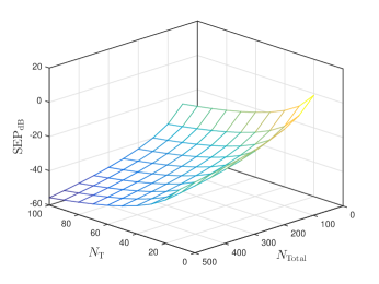
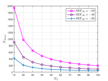
   (a)                                                (b)                                                (c)

Figure 5: Detection performance and CFBG codebook performance; (a) PD and PF versus different $N_{\rm T}N$ and $\gamma$. Note that we can configure $N=1$, that is, one subcarrier in one block, and in this sense, the curves indicate the performance of PD and PF versus $\gamma$ and $N_{\rm T}$; (b) SEP performance versus $N_{\rm T}$ and $N_{\rm Total}$; (c) Tradeoff curves: $N_{\rm Total}$ versus $N_{\rm T}$ under fixed SEP.

VI-C Construction of CFBG Codebook

First, we construct the codebook satisfying the above two principles through a well-known ZFD code proposed in [31]. Its definition is given as follows:

Definition 3.

A ZFD code $\cal C$ with order $m$ is defined by a collection of $C$ $B$-dimensional binary vectors ${\bf c}_{i},1\leq i\leq C$ for which no SP sum ${\bf c}_{1}{{V}}{\bf c}_{2}{{V}}...{{V}}{\bf c}_{k}$ of $k\leq m$ codewords includes any other codeword not used in this sum.

Intuitively, the definition of ZFD code satisfies the Principle 1. Based on the definition, we know that any sum ${\bf c}_{1}{{V}}{\bf c}_{2}{{V}}...{{V}}{\bf c}_{k}$ of $k\leq m$ codewords cannot include the superposition sum of any other codewords, for instance, ${\bf c}_{j_{1}}{{V}}{\bf c}_{j_{2}}{{V}}...{{V}}{\bf c}_{j_{k}},k\leq m$ with $\left\{{{{1,}}\ldots{{,k}}}\right\}\neq\left\{{{{{j}}_{1}}{{,}}\ldots{{,}}{{{j}}_{k}}}\right\}$, since each of the other codewords cannot be included in the sum. Therefore, Principle 2 can be guaranteed by:

Proposition 2.

For a ZFD code $\cal C$ with order $m$, two arbitrary SP sums each of which is superimposed by $k\leq m$ code words are identical if and only if the two codeword sets respectively constituting the two sums are completely identical as well.

Second, we define the concept of BD code satisfying Property 1 by the following:

Definition 4.

A BD code $\cal B$ is the one that has the same codewords as ZFD code but follows ASP sum principle.

Finally, we focus on the construction of two codes and show how to construct the CFBG codebook by integrating the two codes. Let us begin by introducing the ZFD code construction.

VI-C1 Relationship between maximum-distance separable (MDS) and ZFD code and theoretical results

An arbitrary $m$-order ZFD code is constructed on the basis of $m$-order MDS code. We consider a $m$ order $B$-digit ZFD code with the constant weight. Generally, MDS code is an efficient way to construct the ZFD code since each of codewords belonging to MDS code exactly occurs once in the overall code set [32]. Basically, MDS code is a $q$-nary error-correcting code whose codeword digits are members of a set of $q$ basic symbols. MDS code has the maximum possible distance $d=r+1$ for given code size $C=q^{k}$ and codeword length $n=k+r$. A $m$ order $B$-digit ZFD code can be constituted from a $q$-nary ${B\mathord{\left/{\vphantom{Bq}}\right.\kern-1.2pt}q}$-digit MDS code by representing each digit of codeword with a unique weight-one binary $q$-tuple. For example, the $q$-nary symbols 0, 1, . . . $q-1$ are to be replaced by the $q$-digit binary vectors $1,0,\ldots,0$, $0,1,\ldots,0$, $0,0,\ldots,1$ respectively. In this context, the code size satisfies the following relationships:

$$C=q^{k},m={\frac{{{{n}-1}}}{{{k}-{1}}}},q\geq m\left({k-1}\right)\geq 3,n=B\mathord{\left/{\vphantom{Bq}}\right.\kern-1.2pt}q$$ (30)

where $m\in{\mathbb{Z}^{+}},n\in{\mathbb{Z}^{+}}$. Furthermore, $m=3,B=\frac{{{N_{{\rm{Total}}}}{N_{\rm{T}}}}}{{{N_{B}}}}$ has to be satisfied given three wireless nodes at most. The constraint of $2\leq k\leq q-1,2\leq r\leq q-1$ is also imposed due to MDS property [32].

Theorem 2.

The size of MDS based ZFD code satisfies:

$$C={q^{k}},\frac{{{N_{\rm{T}}}}}{{{N_{B}}}}=\frac{{q\left({3k-2}\right)}}{{{N_{{\rm{Total}}}}}},2\leq k\leq\frac{{q+3}}{3},q\geq 3$$ (31)

Proof.

First, since $m=\frac{{n-1}}{{k-1}}=3$ and $n={B\mathord{\left/{\vphantom{Bq}}\right.\kern-1.2pt}q}$ , we can easily derive $\frac{{{N_{\rm{T}}}}}{{{N_{B}}}}=\frac{{q\left({3k-2}\right)}}{{{N_{{\rm{Total}}}}}}$. Then we focus on the range of parameter $k$. Combing $q\geq m\left({k-1}\right)\geq 3$ with $2\leq k\leq q-1$, we can derive $2\leq k\leq\frac{{q+3}}{3}$ when $q\geq 3$ . Furthermore, we consider the constraint $2\leq r\leq q-1$. Since $r=n-k=2k-2$, we have $k\leq\frac{{q+1}}{2}$. Comparing the upper bound $\frac{{q+3}}{3}$ and $\frac{{q+1}}{2}$, we can finally determine the range of $k$ satisfying $2\leq k\leq\frac{{q+3}}{3}$ given $q\geq 3$. The theorem is proved. ∎

Remark 4.

For single-user scenario, $m$ is set to be 2 and the above method still holds true but with the consideration of different parameter configurations. In this case, we can easily have $C={q^{k}},\frac{{{N_{\rm{T}}}}}{{{N_{B}}}}=\frac{{q\left({2k-1}\right)}}{{{N_{{\rm{Total}}}}}},3\leq k\leq\frac{{q+2}}{2},q\geq 4$.

Based on the above theoretical support, we aim to construct the ZFD code in details.

VI-C2 Construction of ZFD code

Firstly, we exploit the concept of Latin hypercubes defined in the following.

Definition 5.

A Latin $k$-dimensional cube of order $q$ is a $k$-dimensional matrix

$${{\bf{L}}^{k,q}}=\left|{{\bf{q}}\left({{i_{1}},{i_{2}},\ldots,{i_{k}}}\right);1\leq{i_{1}},{i_{2}},\ldots,{i_{k}}\leq q}\right|$$ (32)

such that every row is a permutation of the set of natural numbers 1, 2, . . . , q. By a row of ${{\bf{L}}^{k,q}}$ we mean an $q$-tuple of elements ${{\bf{q}}\left({{i_{1}},{i_{2}},\ldots,{i_{k}}}\right)}$ which have identical coordinates $k-1$ at places

Using the definition of Latin hypercube, we then have the definition of orthogonal Latin hypercubes with $N\left(q\right)$ tuples.

Definition 6.

A $N\left(q\right)$-tuple of Latin $k$-dimensional cubes

$$\left[{{\bf{L}}_{l}^{k,q}=\left|{{{\bf{q}}_{l}}\left({{i_{1}},{i_{2}},\ldots,{i_{k}}}\right);1\leq{i_{1}},{i_{2}},\ldots,{i_{k}}\leq q}\right|}\right]$$ (33)

of order $q$ for $l=1,2,\ldots,N\left(q\right)$ is called mutually orthogonal, if whenever ${i_{1}},{i_{2}},\ldots,{i_{k}},i_{1}^{{}^{\prime}},i_{2}^{{}^{\prime}},\ldots,i_{k}^{{}^{\prime}}\in\left\{{1,2,\ldots,q}\right\}$ are such that

$${{\bf{q}}_{l}}\left({{i_{1}},{i_{2}},\ldots,{i_{k}}}\right)={{\bf{q}}_{l}}\left({i_{1}^{{}^{\prime}},i_{2}^{{}^{\prime}},\ldots,i_{k}^{{}^{\prime}}}\right),for\,\,\,all\,1\leq{l}\leq N\left(q\right)$$ (34)

then we must have $i_{i}=i_{i}^{{}^{\prime}}$ for all $i=1,\ldots,k$ . $N\left(q\right)$ represents the maximum number of orthogonal Latin $k$-dimensional cubes of order $q$.

The existence of orthogonal Latin $k$-dimensional cubes of order $q$ can be guaranteed by the following theorem

Theorem 3.

For $\forall k,k\geq 3$ and $\forall q,q\geq 3$, there exists a set of $k$ orthogonal Latin $k$-dimensional cubes of order $q$.

Then, we choose $k=3$ to construct the orthogonal Latin cubes. The relationship between orthogonal Latin cubes and MDS code is given by the following theorem.

Theorem 4.

A $q$-nary MDS code with $C={q^{3}}$ and $d=r+1$ is equivalent to a set of $r$ orthogonal Latin cubes of order $q$ with $q\geq 3,r=N\left(q\right)$.

Proof.

Suppose we have a set of $r$ orthogonal Latin three-dimensional cubes of order $q$. We first number the elements of three independent dimensions of 3-D cubes ( denoted by D1 D2 and D3, respectively) using the same $q$ symbols from which the cubes are formed. Then we construct a ${q^{3}}$ codewords supported code by using D1 for the first position, D2 for the second, D3 for the third and the corresponding cube entries for the remaining $r$ positions. Two codewords with three different digits at the first three positions cannot agree in the last $r$ positions, since each of codewords designed from the orthogonal Latin cubes occurs exactly once. Furthermore, if two code words agree in either two of the first three positions, they can agree in none of the last $r$, since each of the $q$ symbols appears exactly once in any row or column of an arbitrary 2-dimensional slice of Latin cubes. Similarly, if two code words agree in any one of the first three positions, they can also agree in none of the last $r$, since each of the paired $q$ symbols (totally $q^{2}$ symbols) on the 2-dimensional plane of a Latin cube appears exactly once in the set. ∎

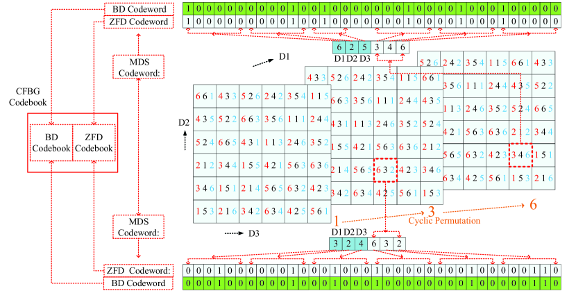
Figure 6: Diagram of CFBG code construction process, including MDS code construction, ZFD code construction and BD code construction. In the beginning, MDS code is constructed through 3 orthogonal 6-order Latin cubes. There exist a total of six Latin cubes that are formulated by performing cyclic permutation for three 6-order orthogonal Latin squares for six times. For each Latin square, each of columns undergoes cyclic permutation simultaneously. Note that a Latin square is a square array in which each row and each column consists of the same set of entries without repetition. Two $n\times n$ $l$-order Latin squares, denoted by ${\bf{X}}=\left[{{x_{ij}}}\right]$ and ${\bf{Y}}=\left[{{y_{ij}}}\right]$, $1\leq{x_{ij}},{y_{ij}}\leq l$, ${x_{ij}},{y_{ij}}\in{{\mathbb{Z}}^{+}}$, are orthogonal iff $n^{2}$ pairs $\left({{x_{ij}},{y_{ij}}}\right)$ are all different. Then ZFD code is constructed as the method mentioned in Theorem 4 and BD code is constructed by copying ZFD code but with different sum principle.

Finally, each MDS codeword is formulated by searching the three dimensions of Latin cubes for the first $k$ digits and then filling out the remnant $r$ positions with the searched value indicated by the three digits in the cube. MDS codeword is further extended as the ZFD codeword by replacing each digit with the corresponding $q$-digit binary vectors.

VI-C3 Construction of CFBG Codebook

After constructing ZFD code, BD code can be obtained according to Definition 4. Thereafter, we formulate a CFBG codebook as follows:

Proposition 3.

A CFBG codebook $\cal G$ is a double-codeword (DCW) codebook defined by:

$$\cal G{\rm{=}}\left\{{\left[{\begin{array}[]{*{20}{c}}{{{\bf{g}}_{{\rm{C}},i}}}&{{{\bf{g}}_{{\rm{B}},i}}}\end{array}}\right]\left|\begin{array}[]{l}{{\bf{g}}_{C,i}}={{\bf{g}}_{B,i}},{{\bf{g}}_{C,i}}\in{\cal C},{{\bf{g}}_{B,i}}\in{\cal B},\\ 1\leq i\leq C\end{array}\right.}\right\}$$ (35)

And the superposition sum of DCWs in $\cal G$ is defined as the two independent superposition sums where the sum between the first columns obeys SP sum principle while that between the second columns follows ASP sum principle.

An example of CFBG construction under order $q=6$ is given in the Fig. 6. As previously introduced, the CFBG codebook is equally divided into two independent codebooks, respectively denoted by $\cal G_{\rm Bob}$ for Bob and $\cal G_{\rm Cha}$ for Charlie. The superposition sum set of codewords in $\cal G$ is defined by:

Definition 7.

The superposition sum set ${\cal G}_{k-1}$ for $k=2,3$ is defined as the collection of all the superposition sums of DCWs in $\cal G$, taken exactly $k$ at a time.

VI-D Codebook Performance

In order to measure the codebook performance, we develop the concept of SEP, that is, the existence probability of duplicate codewords among the decomposed codewords.

Theorem 5.

The SEP of Alice, that is, when Eva randomly selects one codeword in CFBG codebook for randomly-imitating attack, is derived as:

$${\rm SEP}=\frac{{1}}{{{C}}}\propto{\left({\frac{1}{{{N_{{\rm{Total}}}}{N_{\rm{T}}}}}}\right)^{k}},k=3$$ (36)

Proof.

let us consider the number of possible choices of codewords for the three independent nodes. As we know, Eva can attack arbitrary node but Bob and Charlie only focus on their own codebook for distinguishing themselves from each other. Since each codeword is randomly selected, the total number of the choices is equal to $\frac{C}{2}\times\frac{C}{2}\times C$ whereas the duplicate codewords occur with $\frac{C}{2}\times\frac{C}{2}$ possibilities. Therefore, we have ${\rm SEP}=\frac{{1}}{{{C}}}$. Now we know $k=3$ and since $C={q^{k}},\frac{{{N_{\rm{T}}}}}{{{N_{B}}}}=\frac{{q\left({3k-2}\right)}}{{{N_{{\rm{Total}}}}}}$, we can derive the SEP by ${\rm SEP}={\left({\frac{{7{N_{\rm{B}}}}}{{{N_{{\rm{Total}}}}{N_{\rm{T}}}}}}\right)^{3}}$. As shown in Eq. (26), the control variable $N_{\rm B}$ is artificially configured and usually fixed. In this sense, we prove the theorem. ∎

To simulate SEP, $\rm SEP_{dB}$ is defined as follows:

$${\rm{SE}}{{\rm{P}}_{{\rm{dB}}}}=10{\log_{10}}{\rm{SEP}}$$ (37)

We configure $N_{\rm{B}}$ to be 100. Note that at most $N_{\rm T}=100$ antennas are supported in this example. The number of antennas is however not constrained, if needed. Fig. 5(b) shows the value of $\rm SEP_{dB}$ versus $N_{\rm T}$ and $N_{\rm Total}$. As we can see, $\rm SEP_{dB}$ decreases with the increase of $N_{\rm T}$ and $N_{\rm Total}$. This accords with what is shown in Eq. (36). Specifically, the $\rm SEP_{dB}$ reaches -56 under $N_{\rm T}=100$ and $N_{\rm Total}=500$. Fig. 5(c) demonstrates the tradeoff between $N_{\rm T}$ and $N_{\rm Total}$ given the value of $\rm SEP_{dB}$. Obviously, the number of subcarriers occupied for guaranteeing a desirable $\rm SEP_{dB}$ is reduced with the increase of the number $N_{\rm T}$ of antennas. This reduction increases with the decrease of $\rm SEP_{dB}$.

VII Key Technique III: Pilot Encoding $\&$ Decoding

We introduce the pilot encoding and decoding process through the formulated codebook. An example can be shown in Fig. 7. Finally, we will identify the unsolved issues.

Algorithm 1 BDCD Algorithm

0:  Observation codeword $\bf g={\left[{\begin{array}[]{*{20}{c}}{{{\bf{g}}_{{\rm{C}}}}}&{{{\bf{g}}_{{\rm{B}}}}}\end{array}}\right]}$, ${\cal G}_{\rm Bob}$, ${\cal G}_{\rm Cha}$.

0:  Original codewords: ${\bf g}_{{\rm C},1}$, ${\bf g}_{{\rm C},2}$, and ${\bf g}_{{\rm C},3}$.

1:  for $\bf g$ do

2:     In the set ${\cal G}\cup{\cal G}_{1}\cup{\cal G}_{2}$, find the codeword equal to ${{{\bf{g}}_{{\rm{C}}}}}$.

3:     if True then

4:        if Each digit of ${{{{g}}_{{\rm{C}}}}}$ is equal to one  then

5:           Calculate the element ${{{{g}}_{{{\rm{B}},i}}}}$ of ${{{{g}}_{{\rm{B}}}}}$

6:           if There exist $i$ such that ${{{{g}}_{{{\rm{B}},i}}}}=1$ then

7:              Based on Property 1, reduce each digit of ${{{\bf{g}}_{{\rm{C}}}}}$ at the same digit positions by one. Search the resulted codeword in ${\cal G}\cup{\cal G}_{1}\cup{\cal G}_{2}$ again.

8:              if True then

9:                 Indicate jamming attack. Output ${\bf g}_{{\rm C},1}$, ${\bf g}_{{\rm C},2}$.

10:              else

11:                 Indicate no attack. Output ${\bf g}_{{\rm C},1}$, ${\bf g}_{{\rm C},2}$, ${\bf g}_{{\rm C},3}$.

12:              end if

13:           else

14:              Indicate jamming attack. Output ${\bf g}_{{\rm C},1}$, ${\bf g}_{{\rm C},2}$.

15:           end if

16:        else

17:           Interpret $\bf g$ as original codewords using Principle 1& 2.

18:           if Number of decomposed codewords is three then

19:              Output ${\bf g}_{{\rm C},1}$, ${\bf g}_{{\rm C},2}$, ${\bf g}_{{\rm C},3}$.

20:           end if

21:           if Number of decomposed codewords is two then

22:              Eatimate the codeword ${\left[{\begin{array}[]{*{20}{c}}{{{\overline{\bf{g}}}_{{\rm{C}},i,1}}}&{{{\overline{\bf{g}}}_{{\rm{B}},i,1}}}\end{array}}\right]}$ from ${\cal G}_{\rm Bob}$ and ${\left[{\begin{array}[]{*{20}{c}}{{{\overline{\bf{g}}}_{{\rm{C}},i,2}}}&{{{\overline{\bf{g}}}_{{\rm{B}},i,2}}}\end{array}}\right]}$ from ${\cal G}_{\rm Cha}$ . Detect each digit of ${{{\overline{\bf{g}}}_{{\rm{B}},i,1}}}$ and ${{{\overline{\bf{g}}}_{{\rm{B}},i,2}}}$ and calculate the sum of digits respectively as $s_{1}$ and $s_{2}$.

23:              if $s_{1}=s_{2}$ then

24:                 Indicate no error and Output ${{{\overline{\bf{g}}}_{{\rm{C}},i,1}}}$, ${{{\overline{\bf{g}}}_{{\rm{C}},i,2}}}$.

25:              else

26:                 Indicate separation error.

27:              end if

28:           end if

29:        end if

30:     else

31:        Indicate jamming attack. Reduce each digit of $\bf g$ by one and output ${\bf g}_{{\rm C},1}$, ${\bf g}_{{\rm C},2}$ by searching ${\cal G}\cup{\cal G}_{1}\cup{\cal G}_{2}$.

32:     end if

33:  end for

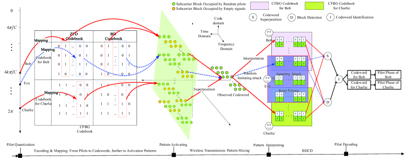
Figure 7: Example of pilot encoding and decoding process by using CFBG DCW codebook under randomly-imitating attack.

VII-1 Pilot Quantization and Encoding

The common phase interval $\left[{0,2\pi}\right)$ is equally quantized into $C$ reference values. Then an one-to-one mapping is formulated between each phase value and a corresponding codeword. Every time Bob (or Charlie) has utilized a random pilot, such as ${\theta_{k_{0}}}$ ( or ${\beta_{k_{0}}}$) at one symbol time (i.e., $k_{0}$) , it compares the phase with reference values, selects the reference value ${\overline{\theta}_{k_{0}}}$ (or ${\overline{\beta}_{k_{0}}}$) closest to the utilized phase and maps the value into a codeword. Finally, two codebooks denoted by $\cal G_{\rm Bob}$ and $\cal G_{\rm Cha}$ are respectively allocated for Bob and Charlie. Bob selects ${\bf g}_{{\rm C},1}$, Charlie selects ${\bf g}_{{\rm C},2}$ and Eva, if existing, selects ${\bf g}_{{\rm C},3}$.

VII-2 Block Pattern Activating

Bob (or Charlie) maps ${\bf g}_{{\rm C},1}$ (or ${\bf g}_{{\rm C},2}$) into the subcarrier block activation patterns. The principle is that Bob (or Charlie) transmits signals on the $i$-th subcarrier block if the $i$-th ($1\leq i\leq B$) row element of ${{\bf{g}}_{{\rm C},1}}$ (${\bf g}_{{\rm C},2}$) is equal to 1, otherwise Bob (or Charlie) keeps silent on this subcarrier block.

VII-3 Block Pattern Interpreting

Due to the overlapping of activation patterns from three nodes, the interpretation of this pattern into original codewords requires the combination of block detection technique and CFBG code. The detailed algorithm is summarized in Algorithm 1.

VII-4 Pilot Decoding Based on Interpreted Codewords

Alice identifies the interpreted codewords as quantized pilot phases, i.e., ${\overline{\theta}_{k_{0}}}$ and ${\overline{\beta}_{k_{0}}}$ and finally recovers the pilot signals.

For this process, what is certain is that three types of attack can be identified perfectly. As to the codeword identification, we will encounter three situations: 1) When Eva keeps silence, two pilots from legitimate nodes can be separated and identified; 2) Under jamming attack, partial pilots, i.e. belonging to Bob and Charlie, can be separated and identified, which is enough for the following channel estimation; 3) Under randomly-imitating attack, we have the following problem:

Problem 5.

Two interpreted codewords within the same codebook, though separated from each other, cannot be identified.

Thanks to CFBG codebook, what we can achieve until now is conveying and separating pilots perfectly while identifying pilots with a certain level of errors. We should note that high-resolution codeword separation logically acts as a necessary step towards high-resolution pilot identification and provides a basis of identification enhancement in the following section.

VIII Key Technique IV: Joint Channel Estimation and Identification

In order to solve above issue and further achieve the critical and final goal, i. e., channel acquisition, we focus on the channel estimation process. Generally, when there is no attack, a well-known LS estimator is enough for channel estimation. Therefore, we in this section turn to the attack environment. We aim to: 1) design the high-precision channel estimator; 2) design a pilot (or channel) identification enhancement mechanism for randomly-imitating attack.

VIII-A Signal Representation for Channel Estimation

We begin our discussion by stacking the signals received within the first three OFDM symbol time as

$${\overline{\bf{Y}}}={\bf{XH}}+{\bf{N}}$$ (38)

Here, we have ${\overline{\bf{Y}}}={\left[{\begin{array}[]{*{20}{c}}{{{\bf{y}}^{\rm{T}}}\left[{{k_{0}}}\right]}&{{{\bf{y}}^{\rm{T}}}\left[{{k_{1}}}\right]}&{{{\bf{y}}^{\rm{T}}}\left[{{k_{2}}}\right]}\end{array}}\right]^{\rm{T}}}$, ${\bf{X}}=\left[{\begin{array}[]{*{20}{c}}{{{\bf{x}}_{\rm{B}}}}&{{{\bf{x}}_{\rm{C}}}}&{{{\bf{x}}_{\rm{E}}}}\end{array}}\right]$ and ${\bf{N}}=\left[{\begin{array}[]{*{20}{c}}{{{\bf{w}}^{\rm{T}}}\left[{{k_{0}}}\right]}&{{{\bf{w}}^{\rm{T}}}\left[{{k_{1}}}\right]}&{{{\bf{w}}^{\rm{T}}}\left[{{k_{2}}}\right]}\end{array}}\right]$. There exist ${{\bf{x}}_{{j}}}={\left[{{x_{{j}}}{{\left[{{k_{i}}}\right]}_{0\leq i\leq 2}}}\right]^{\rm{T}}}\in{{\mathbb{C}}^{3\times 1}}$, $j\in\left\{{{\rm{B,C,E}}}\right\}$ and ${\bf{H}}{\rm{=}}{\left[{\begin{array}[]{*{20}{c}}{{\bf{h}}_{\rm{B}}^{\rm{T}}}&{{\bf{h}}_{\rm{C}}^{\rm{T}}}&{{\bf{h}}_{\rm{E}}^{\rm{T}}}\end{array}}\right]^{\rm{T}}}$. We define ${{\bf{h}}_{{j}}}={{\bf{g}}_{{j}}}\left({{{\bf{I}}_{{N_{\rm{T}}}}}\otimes{\bf{F}}_{\rm{L}}^{\rm{T}}}\right),j\in\left\{{{\rm{B,C,E}}}\right\}$ where ${{\bf{g}}_{{j}}}=\left[{\begin{array}[]{*{20}{c}}{{{\left({{\bf{h}}_{{j}}^{1}}\right)}^{\rm{T}}}}&{,\ldots,}&{{{\left({{\bf{h}}_{{j}}^{{N_{\rm{T}}}}}\right)}^{\rm{T}}}}\end{array}}\right]\in{{\mathbb{C}}^{1\times{N_{\rm{T}}}L}},j\in\left\{{{\rm{B,C,E}}}\right\}$. It is easily to verify ${{\bf{h}}_{{j}}}{\bf{h}}_{{j}}^{\rm{H}}=N{{\bf{g}}_{{j}}}{\bf{g}}_{{j}}^{\rm{H}},j\in\left\{{{\rm{B,C,E}}}\right\}$. Then we define ${\bf{g}}_{{j}}^{\rm{H}}={\left({{{\bf{R}}_{{j}}}\otimes{{\bf{I}}_{L}}}\right)^{\frac{1}{2}}}\widetilde{\bf{g}}_{{j}}^{\rm{H}},j\in\left\{{{\rm{B,C,E}}}\right\}$, where each ${\widetilde{\bf{g}}_{{j}}}\sim{\cal C}{\cal N}\left({0,{{\bf{I}}_{{N_{\rm{T}}}L}}}\right)$ for $j\in\left\{{{\rm{B,C,E}}}\right\}$ is a $1\times N_{\rm T}L$ vector. Finally we derive the relationship between FS and CIR as follows

$${{\bf{h}}_{{j}}}={\widetilde{\bf{g}}_{{j}}}\left({{\bf{R}}_{{j}}^{\frac{1}{2}}\otimes{\bf{F}}_{\rm{L}}^{\rm{T}}}\right),j\in\left\{{{\rm{B,C,E}}}\right\}$$ (39)

From the Lemma B.26 in  [33], we derive the asymptotic approximation for FS channels $j\in\left\{{{\rm{B,C,E}}}\right\}$ by $\frac{1}{{{N_{\rm{T}}}N}}{{\bf{h}}_{{j}}}{\bf{h}}_{{j}}^{\rm{H}}\xlongrightarrow[{N_{\rm{T}}}\to\infty]{\rm{a.s.}}\frac{1}{{{N_{\rm{T}}}}}{\rm{Tr}}\left({{{\bf{R}}_{{j}}}\otimes{{\bf{I}}_{{L}}}}\right)=\frac{L}{{{N_{\rm{T}}}}}{\rm{Tr}}\left({{{\bf{R}}_{{j}}}}\right)$. Similarly, we can obtain the following asymptotic results: $\frac{1}{{{N_{\rm{T}}}N}}{{\bf{h}}_{{j}}}{\bf{h}}_{{l}}^{\rm{H}}\xlongrightarrow[{N_{\rm{T}}}\to\infty]{\rm{a.s.}}0,\forall j\neq l,j,l\in\left\{{{\rm{B,C,E}}}\right\}$, $\frac{1}{{{N_{\rm{T}}}N}}{\bf{w}}\left[{{k_{i}}}\right]{{\bf{w}}^{\rm{H}}}\left[{{k_{j}}}\right]\xlongrightarrow[{N_{\rm{T}}}\to\infty]{\rm{a.s.}}{\sigma^{\rm{2}}},\forall i=j$, and $\frac{1}{{{N_{\rm{T}}}N}}{\bf{w}}\left[{{k_{i}}}\right]{{\bf{w}}^{\rm{H}}}\left[{{k_{j}}}\right]\xlongrightarrow[{N_{\rm{T}}}\to\infty]{\rm{a.s.}}0,\forall i\neq j$. We consider the covariance matrix defined by ${{\bf C}_{\overline{\bf{Y}}}}=\frac{1}{{{N_{\rm{T}}N}}}{\overline{\bf{Y}}}\,{{\overline{\bf{Y}}}}^{\rm{H}}$ satisfying:

$$\mathop{{\bf C}_{\overline{\bf{Y}}}}\xlongrightarrow[{N_{\rm{T}}}\to\infty]{\rm{a.s.}}\frac{L}{{{N_{\rm{T}}}}}{\bf{XR}}{{\bf{X}}^{\rm{H}}}+{\sigma^{2}}{{\bf{I}}_{2}}$$ (40)

where ${\bf{R}}={\rm{diag}}\left\{{\begin{array}[]{*{20}{c}}{{\rm{Tr}}\left({{{\bf{R}}_{\rm{B}}}}\right)}&{{\rm{Tr}}\left({{{\bf{R}}_{\rm{C}}}}\right)}&{{\rm{Tr}}\left({{{\bf{R}}_{\rm{E}}}}\right)}\end{array}}\right\}$

VIII-B Design of Channel Estimator

Using CFBG codebook and demapping operation, Alice derives two separated pilot phases ${\overline{\theta}}_{{k_{0}}}$ and ${\overline{\beta}}_{{k_{0}}}$, and thus deduce the first two columns of $\bf{X}$, denoted by ${\bf{\overline{x}}}_{{i}}$ for the $i$-th column, expressed by: ${{{\bf{\overline{x}}}}_{1}}={\left[{\begin{array}[]{*{20}{c}}{\sqrt{{\rho_{\rm{B}}}}{e^{j{{\overline{\theta}}_{{k_{0}}}}}}}&{\sqrt{{\rho_{\rm{B}}}}{e^{j\left({{{\overline{\theta}}_{{k_{0}}}}+\theta}\right)}}}&{\sqrt{{\rho_{\rm{B}}}}{e^{j\left({{{\overline{\theta}}_{{k_{0}}}}+2\theta}\right)}}}\end{array}}\right]^{\rm{T}}}$, ${{{\bf{\overline{x}}}}_{2}}={\left[{\begin{array}[]{*{20}{c}}{\sqrt{{\rho_{\rm{C}}}}{e^{j{{\overline{\beta}}_{{k_{0}}}}}}}&{\sqrt{{\rho_{\rm{C}}}}{e^{j\left({{{\overline{\beta}}_{{k_{0}}}}+\beta}\right)}}}&{\sqrt{{\rho_{\rm{C}}}}{e^{j\left({{{\overline{\beta}}_{{k_{0}}}}+2\beta}\right)}}}\end{array}}\right]^{\rm{T}}}$ The design principle is to derive FS and CIR based on $\mathop{{\bf C}_{\overline{\bf{Y}}}}$ and ${\bf{\overline{x}}}_{{i}}$.

 

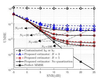
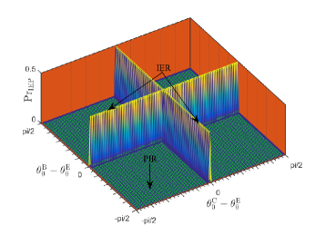
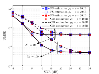
   (a)                                                (b)                                                (c)

Figure 8: Performance evaluation of channel estimation and identification; (a)UMSE versus SNR and $B$; (b)3D plot of IEP versus the mean AoA separations under $N_{\rm T}=64$; (c) UMSE of FS and CIR estimation versus SNR under various power difference.

From Eq. (40), we can derive the MMSE semi-blind estimators for FS channels as ${{\bf{W}}_{\rm{F,B}}}=\sqrt{\frac{{L{\rm{Tr}}\left({{{\bf{R}}_{\rm{B}}}}\right)}}{{{N_{\rm{T}}}}}}{\bf{\overline{x}}}_{\rm{1}}^{\rm{H}}{\bf C}_{{\overline{\bf{Y}}}}^{-1},{{\bf{W}}_{\rm{F,C}}}=\sqrt{\frac{{L{\rm{Tr}}\left({{{\bf{R}}_{\rm{C}}}}\right)}}{{{N_{\rm{T}}}}}}{\bf{\overline{x}}}_{\rm{2}}^{\rm{H}}{\bf C}_{{\overline{\bf{Y}}}}^{-1}$. The estimated versions of FS channels are respectively derived by ${{\widehat{\bf{h}}}_{\rm{B}}}{\rm{=}}{{\bf{W}}_{\rm{F,B}}}{\overline{\bf{Y}}}$ and ${{\widehat{\bf{h}}}_{\rm{C}}}{\rm{=}}{{\bf{W}}_{\rm{F,C}}}{\overline{\bf{Y}}}$. In the following, we first eliminate the influence of FFT weight by multiplying ${{{\widehat{\bf{h}}}_{{j}}}},j\in\left\{{{\rm{B,C}}}\right\}$ by a right-weighting matrix ${{\bf{I}}_{{N_{\rm{T}}}}}\otimes\left\{{{{\left({{\bf{F}}_{\rm{L}}^{\rm{T}}}\right)}^{\rm{H}}}{{\left({{\bf{F}}_{\rm{L}}^{\rm{T}}{\bf{F}}_{\rm{L}}^{\rm{*}}}\right)}^{-1}}}\right\}$. The result is then multiplied by ${\bf{R}}_{{j}}^{-\frac{1}{2}}\otimes{{\bf{I}}_{L}},j\in\left\{{{\rm{B,C}}}\right\}$ to eliminate the influence of spatial correlation. Finally, the CIR estimations are derived as

$${\widehat{\bf{g}}_{{j}}}{\rm{=}}{\widehat{\bf{h}}_{{j}}}\left\{{{\bf{R}}_{{j}}^{-\frac{1}{2}}\otimes\left\{{{{\left({{\bf{F}}_{\rm{L}}^{\rm{T}}}\right)}^{\rm{H}}}{{\left({{\bf{F}}_{\rm{L}}^{\rm{T}}{\bf{F}}_{\rm{L}}^{\rm{*}}}\right)}^{-1}}}\right\}}\right\},j\in\left\{{{\rm{B,C}}}\right\}$$ (41)

VIII-C Identification Enhancement

For randomly-imitating attack, CFBG codebook provides three separated pilots. Three estimated channels can thus be derived using the above same principle. In this context, channel identification is equivalent to pilot identification since each estimator only relies on one corresponding pilot signal. For simplicity, we denote Eva’s pilot signal recovered by:

$${{{\bf{\overline{x}}}}_{3}}={\left[{\begin{array}[]{*{20}{c}}{\sqrt{{\rho_{\rm{E}}}}{e^{j{{\overline{\varphi}}_{{k_{0}}}}}}}&{\sqrt{{\rho_{\rm{E}}}}{e^{j\left({{{\overline{\varphi}}_{{k_{0}}}}+\varphi}\right)}}}&{\sqrt{{\rho_{\rm{E}}}}{e^{j\left({{{\overline{\varphi}}_{{k_{0}}}}+2\varphi}\right)}}}\end{array}}\right]^{\rm{T}}}$$ (42)

where ${\overline{\varphi}}_{{k_{0}}}$ is the recovered pilot phase indicated by the confusing codeword. Its estimation version of CIR satisfies

$${\widehat{\bf{g}}_{\rm{E}}}{\rm{=}}{\widehat{\bf{h}}_{\rm{E}}}\left\{{{\bf{R}}_{\rm{E}}^{-\frac{1}{2}}\otimes\left\{{{{\left({{\bf{F}}_{\rm{L}}^{\rm{T}}}\right)}^{\rm{H}}}{{\left({{\bf{F}}_{\rm{L}}^{\rm{T}}{\bf{F}}_{\rm{L}}^{\rm{*}}}\right)}^{-1}}}\right\}}\right\}$$ (43)

Since CFBG codebook guarantees that Alice can identify which node is under randomly-imitating attack, we turn to design of the identification mechanism for those channels under attack. Take Bob for example, we aim to identify ${\widehat{\bf{g}}_{\rm{B}}}$ and ${\widehat{\bf{g}}_{\rm{E}}}$ by applying maximum-likelihood detection (MLD) and the available spatial correlation. The operation for Charlie, if being misguided, has the same methodology. Note that the probability distribution of ${{\bf{g}}_{\rm{B}}}$ is available at Alice and given in [29] by ${p_{{{\bf{g}}_{\rm{B}}}}}\left({\bf{r}}\right)=\frac{{\exp\left[{-\frac{1}{2}{{\bf{r}}}\left({{\bf{R}}_{\rm{B}}^{-1}\otimes{{\bf{I}}_{L}}}\right){\bf{r}}^{\rm{H}}}\right]}}{{{{\left({2\pi}\right)}^{{{{N_{\rm{T}}}L{\rm{}}}\mathord{\left/{\vphantom{{{N_{\rm{T}}}L{\rm{}}}2}}\right.\kern-1.2pt}2}}}{{\left|{{{\bf{R}}_{\rm{B}}}\otimes{{\bf{I}}_{L}}}\right|}^{{1\mathord{\left/{\vphantom{12}}\right.\kern-1.2pt}2}}}}}$. After deriving the conditional density ${p_{{{\bf{g}}_{{\rm{B}}}}}}\left({{\bf{r}}\left|{{{\bf{R}}_{{\rm{B}}}}}\right.}\right)$ based on ${{\bf{R}}_{{\rm{B}}}}$, we construct the likelihood function ${\rm{In}}\left({{p_{{{\bf{g}}_{{\rm{B}}}}}}\left({{\bf{r}}\left|{{{\bf{R}}_{{\rm{B}}}}}\right.}\right)}\right)$ and formulate the identification problem as $\widehat{\bf{h}}{\rm{=}}\mathop{\arg\max}\limits_{{\bf{r}}={{\widehat{\bf{g}}}_{\rm{B}}},{{\widehat{\bf{g}}}_{\rm{E}}}}\left\{{{\rm{In}}\left({{p_{{{\bf{g}}_{\rm{B}}}}}\left({{\bf{r}}\left|{{{\bf{R}}_{\rm{B}}}}\right.}\right)}\right)}\right\}$ which is then equivalently transformed into

$$\widehat{\bf{h}}{\rm{=}}\mathop{\arg\min}\limits_{{\bf{r}}={{\widehat{\bf{g}}}_{\rm{B}}},{{\widehat{\bf{g}}}_{\rm{E}}}}\left\{{{\bf{r}}\left({{\bf{R}}_{\rm{B}}^{-1}\otimes{{\bf{I}}_{L}}}\right){{\bf{r}}^{\rm{H}}}}\right\}$$ (44)

Then the IEP is finally defined by:

$${\rm Pr_{{IEP}}}=\Pr\left\{{{{\widehat{\bf{g}}}_{\rm{B}}}\left({{\bf{R}}_{\rm{B}}^{-1}\otimes{{\bf{I}}_{L}}}\right)\widehat{\bf{g}}_{\rm{B}}^{\rm{H}}>{{\widehat{\bf{g}}}_{\rm{E}}}\left({{\bf{R}}_{\rm{B}}^{-1}\otimes{{\bf{I}}_{L}}}\right)\widehat{\bf{g}}_{\rm{E}}^{\rm{H}}}\right\}$$ (45)

Proposition 4.

The asymptotic IEP when $N_{\rm T}\to\infty$ is given by:

$${\rm Pr^{\infty}_{{IEP}}}=\Pr\left\{A{{\rm{Tr}}\left({{\bf{R}}_{\rm{B}}^{-2}}\right)>B{\rm{Tr}}\left({{\bf{R}}_{\rm{E}}^{-1}{\bf{R}}_{\rm{B}}^{-1}}\right)}\right\}$$ (46)

where $A=1-{{L{\rm{Tr}}\left({{{\bf{R}}_{\rm{B}}}}\right)\overline{\bf{x}}_{\rm{1}}^{\rm{H}}{\bf{C}}{{\overline{\bf{x}}}_{1}}}\mathord{\left/{\vphantom{{L{\rm{Tr}}\left({{{\bf{R}}_{\rm{B}}}}\right)\overline{\bf{x}}_{\rm{1}}^{\rm{H}}{\bf{C}}{{\overline{\bf{x}}}_{1}}}{{N_{\rm{T}}}}}}\right.\kern-1.2pt}{{N_{\rm{T}}}}},B=1-{{L{\rm{Tr}}\left({{{\bf{R}}_{\rm{C}}}}\right)\overline{\bf{x}}_{{3}}^{\rm{H}}{\bf{C}}{{\overline{\bf{x}}}_{3}}}\mathord{\left/{\vphantom{{L{\rm{Tr}}\left({{{\bf{R}}_{\rm{C}}}}\right)\overline{\bf{x}}_{{3}}^{\rm{H}}{\bf{C}}{{\overline{\bf{x}}}_{3}}}{{N_{\rm{T}}}}}}\right.\kern-1.2pt}{{N_{\rm{T}}}}}$ and ${\bf{C}}={\left({\frac{L}{{{N_{\rm{T}}}}}{\bf{XR}}{{\bf{X}}^{\rm{H}}}+{\sigma^{2}}{{\bf{I}}_{2}}}\right)^{-1}}$.

Proof.

There exists ${\widehat{\bf{g}}_{\rm{B}}}\left({{\bf{R}}_{\rm{B}}^{-1}\otimes{{\bf{I}}_{L}}}\right)\widehat{\bf{g}}_{\rm{B}}^{\rm{H}}={\widehat{\bf{h}}_{\rm{B}}}\left\{{{\bf{R}}_{\rm{B}}^{-2}\otimes\left\{{{{\left({{\bf{F}}_{\rm{L}}^{\rm{T}}}\right)}^{\rm{H}}}{{\left({{\bf{F}}_{\rm{L}}^{\rm{T}}{\bf{F}}_{\rm{L}}^{\rm{*}}}\right)}^{-2}}{\bf{F}}_{\rm{L}}^{\rm{T}}}\right\}}\right\}\widehat{\bf{h}}_{\rm{B}}^{\rm{H}}$. It is easily shown that ${\widehat{\bf{h}}_{\rm{B}}}={{\bf{h}}_{\rm{B}}}-\sqrt{A}{\bf{h}}$ where there exists $A=1-{{L{\rm{Tr}}\left({{{\bf{R}}_{\rm{B}}}}\right){\bf{x}}_{\rm{1}}^{\rm{H}}{\mathbb{E}}\left\{{{\bf C}_{{\overline{\bf{Y}}}}^{-1}}\right\}{{\bf{x}}_{1}}}\mathord{\left/{\vphantom{{L{\rm{Tr}}\left({{{\bf{R}}_{\rm{B}}}}\right){\bf{x}}_{\rm{1}}^{\rm{H}}{{\mathbb{E}}\left\{{{\bf C}_{{\overline{\bf{Y}}}}^{-1}}\right\}}{{\bf{x}}_{1}}}{{N_{\rm{T}}}}}}\right.\kern-1.2pt}{{N_{\rm{T}}}}}$. $\sqrt{A}{\bf{h}}$ is the estimation error that is uncorrelated with ${{\bf{h}}_{\rm{B}}}$. The entries of ${\bf{h}}$ are i.i.d zero-mean complex Gaussian with unity variance. Therefore, we have ${\widehat{\bf{g}}_{\rm{B}}}\left({{\bf{R}}_{\rm{B}}^{-1}\otimes{{\bf{I}}_{L}}}\right)\widehat{\bf{g}}_{\rm{B}}^{\rm{H}}={{\bf{h}}_{\rm{B}}}\overline{\bf{R}}{\bf{h}}_{\rm{B}}^{\rm{H}}-2A{\bf{h}}\overline{\bf{R}}{\bf{h}}_{\rm{B}}^{\rm{H}}+A{\bf{h}}\overline{\bf{R}}{{\bf{h}}^{\rm{H}}}$ where $\overline{\bf{R}}={\bf{R}}_{\rm{B}}^{-2}\otimes\left\{{{{\left({{\bf{F}}_{\rm{L}}^{\rm{T}}}\right)}^{\rm{H}}}{{\left({{\bf{F}}_{\rm{L}}^{\rm{T}}{\bf{F}}_{\rm{L}}^{\rm{*}}}\right)}^{-2}}{\bf{F}}_{\rm{L}}^{\rm{T}}}\right\}$. After simplifying each term using asymptotic approximation, we derive ${\widehat{\bf{g}}_{\rm{B}}}\left({{\bf{R}}_{\rm{B}}^{-1}\otimes{{\bf{I}}_{L}}}\right)\widehat{\bf{g}}_{\rm{B}}^{\rm{H}}\xlongrightarrow[{N_{\rm{T}}}\to\infty]{\rm{a.s.}}L{\rm{Tr}}\left\{{{\bf{R}}_{\rm{B}}^{-1}}\right\}{\rm{+}}A{\rm{Tr}}\left\{{\overline{\bf{R}}}\right\}$. Similarly, we have ${\widehat{\bf{g}}_{\rm{E}}}\left({{\bf{R}}_{\rm{E}}^{-1}\otimes{{\bf{I}}_{L}}}\right)\widehat{\bf{g}}_{\rm{E}}^{\rm{H}}\xlongrightarrow[{N_{\rm{T}}}\to\infty]{\rm{a.s.}}L{\rm{Tr}}\left\{{{\bf{R}}_{\rm{B}}^{-1}}\right\}+B{\rm{Tr}}\left\{{\widetilde{\bf{R}}}\right\}$ where $\widetilde{\bf{R}}={\bf{R}}_{\rm{E}}^{-\frac{1}{2}}{\bf{R}}_{\rm{B}}^{-1}{\bf{R}}_{\rm{E}}^{-\frac{1}{2}}\otimes\left\{{\left({{\bf{F}}_{\rm{L}}^{\rm{T}}}\right)^{\rm{H}}}{\left({{\bf{F}}_{\rm{L}}^{\rm{T}}{\bf{F}}_{\rm{L}}^{\rm{*}}}\right)^{-2}}{\bf{F}}_{\rm{L}}^{\rm{T}}\right\}$. Based on those equations, the proposition can be easily proved. ∎

We use the asymptotic analysis as a tool to provide tight approximations for finite $N_{\rm T}$ [33]. As shown in Fig. 8(b), not very large antenna, i.e., $N_{\rm T}=64$, can bring the precise decision. For massive MIMO systems, generally with antennas of 128 or more, those asymptotic approximation results are precise enough for our calculation. Proposition 4 provides a mathematical support of the theoretical limit that pilot identification enhancement can bring under randomly-imitating attack.

In what follows, we stimulate the performance of channel estimation and identification using proposed estimators. We consider uniform linear array (ULA) with spacing $d=\lambda/2$ and $N_{\rm T}\geq 8$. All the spatial correlation matrices are generated such that the spatial correlation between any two antennas at each path can be given by $\rho\left({{\theta_{0}},d}\right){\rm{=}}\int_{-\pi}^{\pi}{{e^{\frac{{-j2\pi d\sin\left({\theta-{\theta_{0}}}\right)}}{\lambda}}}}P\left({\theta-{\theta_{0}}}\right)d\theta$ where $\theta_{0}$ denotes the mean AoA and $P$ denotes the channel power angle spectrum (PAS) that is modeled by Truncated Gaussian distribution [34, 35]. The mean AoA of Bob, Charlie and Eva, respectively denoted by $\theta^{\rm B}_{0}$, $\theta^{\rm C}_{0}$ and $\theta^{\rm E}_{0}$, are generated independently and distributed identically within $[-\pi,\pi]$. For the channel estimation part, we consider $N_{\rm Total}=128$ subcarriers are occupied by pilot tones. We assume Bob and Charlie have the same transmission power, i. e., $\rho_{\rm{B}}=\rho_{\rm{C}}=\rho$ and define ${\rm{SNR}}={{{P}}\mathord{\left/{\vphantom{{{P}}{{\sigma^{2}}}}}\right.\kern-1.2pt}{{\sigma^{2}}}}$. We also define the user average MSE (UMSE) of FS and CIR estimation respectively as ${{{\mathbb{E}}\left\{{{{\left\|{{{\widehat{\bf{h}}}_{\rm{B}}}-{{\bf{h}}_{\rm{B}}}}\right\|}^{2}}+{{\left\|{{{\widehat{\bf{h}}}_{\rm{C}}}-{{\bf{h}}_{\rm{C}}}}\right\|}^{2}}}\right\}}\mathord{\left/{\vphantom{{E\left\{{{{\left\|{{{\widehat{\bf{h}}}_{\rm{B}}}-{{\bf{h}}_{\rm{B}}}}\right\|}^{2}}+{{\left\|{{{\widehat{\bf{h}}}_{\rm{C}}}-{{\bf{h}}_{\rm{C}}}}\right\|}^{2}}}\right\}}{2N{N_{\rm{T}}}}}}\right.\kern-1.2pt}{2N{N_{\rm{T}}}}}$ and ${{{\mathbb{E}}\left\{{{{\left\|{{{\widehat{\bf{g}}}_{\rm{B}}}-{{\bf{g}}_{\rm{B}}}}\right\|}^{2}}+{{\left\|{{{\widehat{\bf{g}}}_{\rm{C}}}-{{\bf{g}}_{\rm{C}}}}\right\|}^{2}}}\right\}}\mathord{\left/{\vphantom{{E\left\{{{{\left\|{{{\widehat{\bf{g}}}_{\rm{B}}}-{{\bf{g}}_{\rm{B}}}}\right\|}^{2}}+{{\left\|{{{\widehat{\bf{g}}}_{\rm{C}}}-{{\bf{g}}_{\rm{C}}}}\right\|}^{2}}}\right\}}{2N{N_{\rm{T}}}}}}\right.\kern-1.2pt}{2N{N_{\rm{T}}}}}$. For the identification simulations, since Eva can flexibly choose to attack any nodes, we define the identification error region (IER) as the set of all the collections of $\left({\theta_{0}^{\rm{B}}-\theta_{0}^{\rm{E}},\theta_{0}^{\rm{C}}-\theta_{0}^{\rm{E}}}\right)$ such that ${\rm Pr_{{IEP}}}>0$ is satisfied for Bob and/or Charlie. Correspondingly, the perfect identification region (PIR) is defined as the set making ${\rm Pr_{{IEP}}}=0$.

Fig. 8(a) presents the UMSE performance of CIR estimation versus SNR and different number $B$ of subcarrier blocks. $L$ is configured to be 6 and Eva is assumed to be with same SNR as Bob and Charlie. As we can see, traditional pilot spoofing attack causes a high-UMSE floor on CIR estimation for Bob and Charlie. However, the proposed mechanism breaks down this floor and its UMSE gradually decreases with the increase of transmit antennas. Moreover, we find that the UMSE under proposed estimators approaches the level under perfect MMSE with the increase of antennas. On the other hand, the case without quantization serves as an another performance benchmark. It can be shown that the UMSE gradually decreases with the increase of $B$ and $B=5$ is enough to guarantee Alice a desirable UMSE, like the one under no quantization.

Fig. 8(b) shows the IEP versus the mean AoA separation under $N_{\rm T}=64$. The simulation is averaged over 1000 runs, each of which performs 1000 channel average. As we can see, IER is composed by the special points for which at least one of its axes has zero value. It means that the available PIR can be extensively achieved unless any legitimate node has the same average AoA as Eva. Fig. 8(c) shows the UMSE performance of FS and CIR estimation versus SNR under various power difference relative to Eva. $L$ is configured to be 8 and ${B}$ is set to be 5. As we can see, the UMSE is not influenced by the power of Eva, even with $30\rm dB$ larger than Bob or Charlie, under both $N_{\rm T}=100$ and $N_{\rm T}=8$. The reason is that the interference can be eliminated naturally from the received signal space when the dimension of signals observed is no more than the number of OFDM symbol time in use.

IX Conclusions

In this paper, we designed a CFBG based PA mechanism for a two-user OFDM system to protect the channel estimation over frequency-selective channels. In this scheme, the values of pilot tones were randomized to avoid the pilot-spoofing attack but also cause a serious hybrid attack. To resolve those problems in a unique framework, a scheme combing detection, coding and channel estimation was devised to achieve secure PA with low SEP and IEP as well as high-accuracy channel estimation. Some interesting results were presented to verify the robustness of proposed scheme under hybrid attack modes.

References

• [1] U. M. Maurer, “Authentication theory and hypothesis testing,” IEEE Trans. Inf. Theory, vol. 46, no. 4, pp. 1350-1356, July 2000.
• [2] P. K. Gopala, L. Lai, and H. El Gamal, “On the secrecy capacity of fading channels,” IEEE Trans. Inf. Theory, vol. 54, no. 10, pp. 4687-4698, Oct. 2008.
• [3] D. Xu, P. Ren, and J. A. Ritcey, “Optimal grassmann manifold eavesdropping: A huge security disaster for M-1-2 wiretap channels," accepted in IEEE GLOBECOM, Dec. 2017.
• [4] Y. Wu, C. Xiao, Z. Ding, X. Gao, and S. Jin, “Linear precoding for finitealphabet signaling over MIMOME wiretap channels," IEEE Trans. Veh. Technol., vol. 61, no. 6, pp. 2599-2612, Jul. 2012.
• [5] D. Xu, P. Ren, and J. A. Ritcey, “Artificial-noise-resistant eavesdropping in MISO wiretap channels: Receiver construction and performance analysis," accepted in IEEE VTC-Fall, Sept. 2017.
• [6] Y.-S. Shiu, S.-Y. Chang, H.-C. Wu, S.-H. Huang, and H.-H. Chen, “Physical layer security in wireless networks: A tutorial,” IEEE Wireless Commun., vol. 18, no. 2, pp. 66-74, Apr. 2011.
• [7] P. L. Yu, J. S. Baras, and B. M. Sadler, “Physical-layer authentication,” IEEE Trans. Inf. Forensics and Security, vol. 3, no. 1, pp. 38-51, Mar. 2008.
• [8] D. Xu, P. Ren, Q. Du, L. Sun, and Y. Wang, “Weighted-Voronoi-diagram based codebook design against passive eavesdropping for MISO systems," accepted in IEEE VTC-Spring, June 2017.
• [9] D. Xu, P. Ren, Q. Du, and L. Sun, “Hybrid secure beamforming and vehicle selection using hierarchical agglomerative clustering for C-RAN-based vehicle-to-Infrastructure communications in vehicular cyber-physical systems," Int. J. Distrib. Sens. Netw., vol. 12, no. 8, Aug. 2016.
• [10] A. Mukherjee, S. Fakoorian, J. Huang, and A. L. Swindlehurst, “Principles of physical layer security in multiuser wireless networks: A survey,” IEEE Commun. Surveys Tuts., vol. 16, no. 3, pp. 1550-1573, Aug. 2014.
• [11] X. Wang, P. Hao, and L. Hanzo, “Physical-layer authentication for wireless security enhancement: Current challenges and future developments,” IEEE Commun. Mag., vol. 54, no. 6, pp. 152-158, Jun. 2016.
• [12] C. Shahriar, M. La Pan, M. Lichtman, T. C. Clancy, R. McGwier, R. Tandon, S. Sodagari, and J. H. Reed, “PHY-Layer resiliency in OFDM communications: A tutorial," IEEE Commun. Surveys Tuts., vol. 17, no. 1, pp. 292-314, Aug. 2015.
• [13] D. Xu, Q. Du, P. Ren, L. Sun, W. Zhao, and Z. Hu, “AF-based CSI feedback for user selection in multi-user MIMO systems," in Proc. IEEE GLOBECOM, Dec. 2015, pp. 1-6.
• [14] D. Xu, P. Ren, Q. Du, L. Sun, and Y. Wang, “Towards win-win: weighted-Voronoi-diagram based channel quantization for security enhancement in downlink cloud-RAN with limited CSI feedback," Sci. China Inf. Sci., vol. 60, no. 4, pp. 1-17, Mar. 2017.
• [15] M. Ozdemir and H. Arslan, “Channel estimation for wireless OFDM systems," IEEE Commun. Surveys Tuts., vol. 9, no. 2, pp. 18-48, 2nd Quart. 2007.
• [16] D. Xu, P. Ren, Y. Wang, Q. Du, and L. Sun, “ICA-SBDC: A channel estimation and identification mechanism for MISO-OFDM systems under pilot spoofing attack," in Proc. IEEE ICC, May 2017, pp. 1-6.
• [17] D. Xu, P. Ren, J. A. Ritcey, H. He, and Q. Xu, “ICA-based channel estimation and identification against pilot spoofing attack for OFDM systems," accepted in IEEE WCNC 2018, Apr. 2018.
• [18] X. Zhou, B. Maham, and A. Hjorungnes, “Pilot contamination for active eavesdropping," IEEE Trans. Wireless Commun., vol. 11, no. 3, pp. 903-907, Mar. 2012.
• [19] D. Kapetanovic, G. Zheng, K.-K. Wong, and B. Ottersten, “Detection of pilot contamination attack using random training and massive MIMO," in Proc. IEEE PIMRC, Sep. 2013, pp. 13-18.
• [20] J. K.Tugnait, “Self-contamination for detection of pilot contamination attack in multiple antenna systems,” IEEE Wireless Commun. Letters, vol. 4, no. 5, pp. 525-528, Oct. 2015.
• [21] Q. Xiong, Y.-C. Liang, K. H. Li, and Y. Gong, “An energy-ratio-based approach for detecting pilot spoofing attack in multiple-antenna systems,” IEEE Trans. Inf. Forensics and Security, vol. 10, no. 5, pp. 932-940, May 2015.
• [22] Q. Xiong, Y.-C. Liang, K. H. Li, and Y. Gong, “A two-way training method for defending against pilot spoofing attack in MISO systems," in Proc. IEEE ICC, June 2015, pp. 1880-1885.
• [23] D. Kapetanovic, A. Al-Nahari, A. Stojanovic, and F. Rusek, “Detection of active eavesdroppers in massive MIMO,” in Proc. IEEE PIMRC, Sep. 2014, pp. 585-589.
• [24] Y. Wu, R. Schober, D. W. K. Ng, C. Xiao, and G. Caire, “Secure massive MIMO transmission with an active eavesdropper,” IEEE Trans. Inf. Theory, vol. 62, no. 7, pp. 3880-3900, Jul. 2016.
• [25] J.K. Tugnait,“On mitigation of pilot spoofing attack,” in Proc. 2017 IEEE Int. Conf. Acous. Speech Signal Proc., March 2017.
• [26] M. Litchman, J. D. Poston, S. Amuru, C. Shahriar, T. C. Clancy, R. M. Buehrer, and J. H. Reed, “A communications jamming taxonomy," IEEE Security and Privacy, vol. 14, no. 1, pp. 47-54, Jan. 2016.
• [27] T. C. Clancy and N.Georgen, “Security in cognitive radio networks: threats and mitigations," in Proc. 3rd Int. Conf. CrownCom., May 2008, pp. 1-8.
• [28] C. Shahriar and T. C. Clancy, “Performance impact of pilot tone randomization to mitigate OFDM jamming attacks," in Proc. IEEE CCNC, Jan. 2013, pp. 813-816.
• [29] N.Goodman, “Statistical analysis based on a certain multivariate complex Gaussian distribution (an introduction)," Ann. Math. Statist., vol. 34, no. 1, pp. 152-177, Mar. 1963.
• [30] M. Z. Shakir, A. Rao, and M.-S. Alouini, “On the decision threshold of eigenvalue ratio detector based on moments of joint and marginal distributions of extreme eigenvalues,” IEEE Trans. Wireless Commun., vol. 12, no. 3, pp. 974-983, Mar. 2013.
• [31] W. H. Kautz and R. C. Singleton, “Nonrandom binary superimposed codes,” IEEE Trans. Inf. Theory, vol. 10, no. 4, pp. 363-377, Oct. 1964.
• [32] R. C. Singleton, “Maximum distance q-nary codes” IEEE Trans. Inf. Theory, vol. 10, no. 2, pp. 116-118, Apr. 1964.
• [33] Z. D. Bai and J. W. Silverstein, Spectral Analysis of Large Dimensional Random Matrices, 2nd ed. Springer Series in Statistics, New York, NY, USA, 2009.
• [34] Y. S. Cho, J. Kim, W. Y. Yang, and C. G. Kang, MIMO-OFDM Wireless Communications with MATLAB, Singapore: John Wiley & Sons, 2010.
• [35] D. Xu, P. Ren, Q. Du, and L. Sun, “Joint dynamic clustering and user scheduling for downlink cloud radio access network with limited feedback," China Communications, vol. 12, no. 12, pp. 147-159, Dec. 2015.