Alternative explanations for extreme supersolar iron abundances inferred from the energy spectrum of Cygnus X-1

Abstract

Here we study a 1–200 keV energy spectrum of the black hole binary Cygnus X-1 taken with NuSTAR and Suzaku. This is the first report of a NuSTAR observation of Cyg X-1 in the intermediate state, and the observation was taken during the part of the binary orbit where absorption due to the companion’s stellar wind is minimal. The spectrum includes a multi-temperature thermal disk component, a cutoff power-law component, and relativistic and non-relativistic reflection components. Our initial fits with publicly available constant density reflection models (relxill and reflionx) lead to extremely high iron abundances ($>$9.96 and $10.6^{+1.6}_{-0.9}$ times solar, respectively). Although supersolar iron abundances have been reported previously for Cyg X-1, our measurements are much higher and such variability is almost certainly unphysical. Using a new version of reflionx that we modified to make the electron density a free parameter, we obtain better fits to the spectrum even with solar iron abundances. We report on how the higher density ($n_{e}=(3.98^{+0.12}_{-0.25})\times 10^{20}$ cm^-3) impacts other parameters such as the inner radius and inclination of the disk.

1. Introduction

The bright black hole (BH) high mass X-ray binary Cygnus X-1 has been key for many of the advances in our knowledge of accreting BHs. A mass measurement of the compact object showing that it is well above the maximum mass allowed for a neutron star ($>$3$\,M_{\mathord{\odot}}$) provided the first evidence that such compact objects exist (Gies & Bolton, 1986). The fact that BHs enter into different spectral states, such as the soft and hard states, was first demonstrated with observations of Cyg X-1 (Tananbaum et al., 1972). Cyg X-1 is one of two sources where it has been possible to show that the compact jet, which is seen in the hard state, is an extended radio feature (Stirling et al., 2001). Cyg X-1 is also known to have a strong power-law component in its spectrum extending to at least a few MeV (McConnell et al., 2002) with a very high level ($\sim$70%) of polarization (Laurent et al., 2011; Jourdain et al., 2012), possibly indicating that the emission above 400 keV is dominated by synchrotron emission from the jet.

The properties of Cyg X-1 are very well-constrained compared to most BH binaries. It has a parallax distance measurement of $1.86^{+0.12}_{-0.11}$ kpc (Reid et al., 2011), which is consistent with a dust-scattering measurement (Xiang et al., 2011). Optical and near-IR observations made over its 5.6 day orbit constrain the BH mass to be $14.8\pm 1.0$$\,M_{\mathord{\odot}}$ and its binary inclination to be $27.1^{\circ}\pm 0.8^{\circ}$ (Orosz et al., 2011). The spin of the BH has been constrained using two techniques: modeling the thermal continuum and the reflection component. The measurements agree that the spin of the BH is high. The continuum technique gives a value for the spin ($a_{*}>0.983$, 3-$\sigma$ limit), which is consistent with being maximal or very slightly below maximal (Gou et al., 2014), while the reflection measurements allow for somewhat more modest spin (Duro et al., 2011; Miller et al., 2012; Fabian et al., 2012; Tomsick et al., 2014; Walton et al., 2016). For example, using four observations, Walton et al. (2016) find a range of $a_{*}$ values from 0.93 to 0.96. One reason that the Walton et al. (2016) values are a little lower than the Gou et al. (2014) values is that Gou et al. (2014) assume that the inner disk is aligned with the orbital plane.

The Gou et al. (2014) and Walton et al. (2016) spin measurements occur when the source is in the soft state and rely on the assumption that the disk extends to the innermost stable circular orbit (ISCO). Measurements of Cyg X-1 and other systems, such as LMC X-3 (Steiner et al., 2010), provide good evidence that the disk extends to the ISCO in the soft state. However, the situation is less clear in the hard and intermediate states. For the hard state, it is predicted that thermal conduction of heat from the corona will cause the inner disk to evaporate (Meyer, Liu & Meyer-Hofmeister, 2000), leading to an optically thick and geometrically thin disk that is truncated at some significant distance away from the black hole. While there is evidence for truncation at luminosities near 0.1% of the Eddington limit ($L_{\rm Edd}$) for GX 339–4 (Tomsick et al., 2009), measurements of the reflection component in the bright hard state ($\mathrel{\lower 3.44444pt\hbox{\hbox to0.0pt{$\sim$\hss}\raise 3.87495pt\hbox{$>$} }}$5% $L_{\rm Edd}$) often lead to estimates of inner radii very close to the ISCO for several sources, including GRS 1739–278 (Miller et al., 2015). The luminosity of Cyg X-1 is typically 0.8–2.8% $L_{\rm Edd}$, using 0.1–500 keV unabsorbed fluxes (Yamada et al., 2013), and even with high quality data from the Nuclear Spectroscopic Telescope Array (NuSTAR) and Suzaku, there have been conflicting results concerning whether the disk in the hard state is truncated or not (Parker et al., 2015; Basak et al., 2017).

Given that the binary inclination for Cyg X-1 has been measured to high precision, it is also interesting to compare the inner disk inclinations inferred from reflection measurements to the binary value ($27.1^{\circ}\pm 0.8^{\circ}$). In the soft state, Tomsick et al. (2014) found an inner disk inclination $>$40^∘, and Walton et al. (2016) reported values between $38^{\circ}$ and $41^{\circ}$ for four different soft state measurements. Taken at face value, the data suggest a disk warp of 10–15^∘, which has important implications for BH formation since it is very likely that the BH would need to be formed with its spin misaligned from the binary plane to produce this warp (Bardeen & Petterson, 1975; Schandl & Meyer, 1994; Fragile et al., 2007). Another implication is that the Cyg X-1 BH would need to be born with its rapid rotation rate (as described above, $a_{*}=0.93$–0.96 for a warped disk or $a_{*}>0.983$ if the entire disk is aligned with the orbital plane).

Another surprising result from the reflection fits for Cyg X-1 as well as GX 339–4 is the measurement of high iron abundances. For example, Walton et al. (2016) find a value of $A_{\rm Fe}=4.0$–4.3 times solar for Cyg X-1, and Parker et al. (2015) find $A_{\rm Fe}=4.7\pm 0.1$. For GX 339-4, values of $A_{\rm Fe}=5\pm 1$ and $6.6^{+0.5}_{-0.6}$ have been found (García et al., 2015; Parker et al., 2016). Fürst et al. (2015) also obtain high values of $A_{\rm Fe}$ for GX 339–4, but they find that the abundances change significantly for different assumptions about the continuum fitting. V404 Cyg is another black hole system where reflection fits have resulted in supersolar abundances of $A_{\rm Fe}=2$–5 (Walton et al., 2017).

While there have been previous reports of NuSTAR and Suzaku observations of Cyg X-1 in the soft state and the hard state (Tomsick et al., 2014; Parker et al., 2015; Walton et al., 2016; Basak et al., 2017), the work in this paper presents the first analysis of contemporaneous observations of Cyg X-1 in the intermediate state with these satellites. As the name implies, the intermediate state has luminosities and spectral parameters (such as disk temperatures and power-law slopes) that are in between the soft and hard states, and it may provide clues to how sources in general and Cyg X-1 in particular make transitions between soft and hard states. The Cyg X-1 stellar wind can cause significant absorption of the X-ray spectrum, including distortion of the iron line (Tomsick et al., 2014; Walton et al., 2016), but the time of the intermediate state observation was carefully chosen to occur at the orbital phase when the BH is in front of the companion to minimize the absorption. In section 2, we describe the observations and how the data were analyzed. Section 3 includes the results of the spectral fitting, and the results are discussed in Section 4.

2. Observations and Data Reduction

We observed Cyg X-1 with NuSTAR (Harrison et al., 2013) and Suzaku (Mitsuda et al., 2007) on 2015 May 27–28 (MJD 57,169–57,170). Light curves measured by the Monitor of All-sky X-ray Image (MAXI; Matsuoka et al., 2009) and the Swift Burst Alert Telescope (BAT; Krimm et al., 2013) in the 2–20 and 15–50 keV energy bands, respectively, are shown in Figure 1. They cover the time of the observation that we are focusing on in this work as well as the earlier hard state observation reported on in Parker et al. (2015) and Basak et al. (2017). The BAT count rate was similar for the two observations, but the 2–20 keV MAXI count rate was higher during the 2015 May observation. Grinberg et al. (2013) used Cyg X-1 data from all-sky monitors, including MAXI, to define count rates for different states. The weighted average of the count rates for MAXI measurements within 3 days of the 2015 May observation gives 2–4 and 4–10 keV rates of $1.032\pm 0.011$ and $0.654\pm 0.006$ s^-1, respectively, and the ratio of the 4–10 to 2–4 keV rates is $0.633\pm 0.009$. These values indicate that Cyg X-1 was in the intermediate state during the 2015 May observation. The states are indicated in Figure 1.

Table 1 provides information about the NuSTAR and Suzaku observations used in this work, the observation identifier numbers (ObsIDs), the start and stop times of the observations, and the exposure times obtained. The middle of the observation is close to the orbital phase corresponding to the superior conjunction of the supergiant, and the range of orbital phases covered is 0.42–0.56. This was planned in order to minimize absorption due to stellar wind material. In the following, we describe the reduction of the data from each mission in more detail.

2.1. NuSTAR

We processed the data for the two NuSTAR focal plane modules (FPMA and FPMB) using HEASOFT v6.21, NUSTARDAS v1.7.0, and version 20170503 of the NuSTAR calibration data base (CALDB). We produced cleaned event files using nupipeline and then light curves and spectra using nuproducts. For light curves and spectra, we used a circular source extraction region with a radius of $180^{\prime\prime}$ and a circular background region with a radius of $90^{\prime\prime}$. Due to the brightness of Cyg X-1, the background region was placed on a corner of the NuSTAR field of view away from the source. We rebinned the spectra with the requirement that the source is detected at the 30-$\sigma$ level or higher in each bin.

The 3–79 keV light curve (Figure 2a) shows variability in the FPMA+FPMB count rate with the lowest 50 s bin having a rate of 493 s^-1 and the highest having 834 s^-1. However, the hardness (Figure 2b), which is the ratio of the 10–79 to the 3–10 keV rates, shows very little variation, indicating that the energy spectrum is relatively stable during the observation. While NuSTAR observed the source for $\sim$36 ks, the actual livetime was $\sim$20 ks (Table 1).

2.2. Suzaku

For the X-ray Imaging Spectrometers (XIS0, XIS1, and XIS3; Koyama et al., 2007), we used the 1/4 window mode, which has a CCD readout time of 2 s. Also, due to the brightness of the source, we specified a burst mode to reduce photon pile-up, causing the CCD to be exposed for 0.3 s of each 2 s window. However, the detectors were not put in burst mode for the first 19 ks of the observation, making this part of the observation is not usable. The livetimes listed in Table 1 for the XIS units are also affected by filtering out times when the count rates were high enough to produce telemetry saturation. It is this filtering that causes the livetimes to be significantly different for the individual XIS units.

We reprocessed the XIS data using aepipeline and version 20160607 of the CALDB to make new event lists. We then made a new good time interval (GTI) file and applied it to the event lists to filter out the first 19 ks of the observation. We used aeattcor2 to calculate attitude corrections and applied the corrections with xiscoord. Even with the burst mode, there is significant photon pile-up. We calculated the level of pile-up in each pixel using pileest, and made a source extraction region that does not include the inner part of the point spread function. We excluded data from an inner circular region so that all the data that we did include comes from pixels where the pile-up fraction is less than 4%. The other criterion for a pixel to be included in the source extraction region is that it is within $4^{\prime}$ of the source position. For background subtraction, we extracted a spectrum from rectangular regions that are as far as possible from the source. We made response matrices for each XIS unit using xisrmfgen and xissimarfgen. XIS0 and XIS3 have very similar responses because they are both front-illuminated CCDs, and we combined them for spectral fitting. As in Tomsick et al. (2014), we added 2% systematic uncertainties in quadrature with the statistical uncertainties. We rebinned the spectra with the requirement that the source is detected at the 20-$\sigma$ level or higher in each bin.

The hard X-ray detector (HXD; Takahashi et al., 2007) does not have imaging capabilities and consists of two kinds of detectors: Silicon PIN diodes covering 12–70 keV and GSO scintillators covering 40–600 keV. After 2014, Suzaku operation suffered from degradation of the power supply system, including the Solar Array Panel (SAP) and batteries. For the observations from 2014 until the end of the mission, it was difficult to use both XIS and HXD in most cases. However, we did use both instruments for the Suzaku observation in 2015 May. The observation started at 11:23 (UT) on May 27, but the HXD detector parameters were not set properly until 17:15 on May 27 (UT) due to the recovery from an “Under Voltage Control” or UVC event. Hence, we excluded the data during this period. In addition, to save satellite power, HXD was sometimes turned off, leading to a net HXD exposure of 18.6 ks. Cyg X-1 was observed at the XIS nominal position, i.e., 3.5^′ offset from the HXD optical axis. The HXD deadtime-corrected spectra were obtained in the standard manner using standard FTOOLs hxdpinxbpi and hxdgsoxbpi for PIN and GSO, respectively. For both PIN and GSO source spectra, a 1% systematic error was added for each spectral bin (e.g., Torii et al., 2011). The predicted non X-ray background (NXB) was produced from files at the public ftp sites. To estimate the systematic error on the GSO background, we compared the data during the Earth-occultation period to the model for the background. The difference between the data during occultation and the model lead to an estimate of 5% systematic error on the GSO background, and we included this during spectral fitting. For PIN, we further subtracted the cosmic X-ray background (CXB) based on previous observations (Gruber et al., 1999). We used the PIN spectrum from 15–55 keV except for the 40–45 keV range due to the Gd K line structure (see Kouzu et al., 2013). For GSO, we used data in the 82–192 keV band, with the upper end of the range being set by the statistical quality of the spectrum. In the spectral fitting, we used the following energy responses: ae_hxd_pinxinome11_20110601.rsp for PIN and ae_hxd_gsoxinom_20100524.rsp with an additional correction file (ae_hxd_gsoxinom_crab_20100526.arf) for GSO.

3. Results

We initially fitted the NuSTAR+Suzaku energy spectrum with a model consisting of a multi-temperature thermal disk (diskbb) component (Mitsuda et al., 1984) and a power-law. We also included interstellar absorption using v2.3.2 of the tbnew model and a multiplicative constant to allow for differences in normalization between the six spectra (XIS0+XIS3, XIS1, FPMA, FPMB, PIN, and GSO). For modeling the absorption, we used Wilms, Allen & McCray (2000) abundances and Verner et al. (1996) cross sections. A very poor fit is obtained with $\chi^{2}=29,415$ for $\nu=2759$ degrees of freedom (dof). Figure 3 shows the data-to-model ratio residuals for this model. In each case, the Suzaku and NuSTAR spectra were fitted simultaneously, but we show two panels per model so that the data from each instrument is visible. The residuals for the diskbb+powerlaw model (see Figures 3a₁ and 3a₂) show the hallmarks of relativistic Compton reflection with positive features at the Fe K$\alpha$ transition energies and in the 20–100 keV range. In the reflection scenario, these features are identified as fluorescence of iron in the accretion disk (Fabian et al., 1989) and the “Compton hump” (Lightman & White, 1988). The negative residuals in the $\sim$8–15 keV range are partly due to the surrounding positive features and partly caused by a relativistically smeared Fe absorption edge.

Replacing the power-law with a relxill component leads to a huge improvement in the fit (to $\chi^{2}/\nu=3715/2751$). The relxill model includes a direct power-law with an exponential cutoff as well as the reflection component predicted when a cutoff power-law is incident on an optically thick accretion disk. The calculation of the reflection component is based on the xillver model (García et al., 2013, 2014), which includes continuum, emission lines, and absorption edges. This component is then relativistically smeared, including the effects of the relline convolution calculation (Dauser et al., 2013). In this paper, we used v1.0.0 of the relxill model. Although the residuals shown in Figures 3b₁ and 3b₂ are much improved, there is evidence for a narrow iron emission line, which has been seen previously (Miller et al., 2002; Walton et al., 2016), and is likely due to X-ray irradiation of the companion star, the stellar wind material, or the outer disk.

Assuming that the narrow line is caused by irradiation of some cool material in the system, it is physically reasonable to assume that it is part of a full reflection component, motivating the addition of a xillver component to the model. A model consisting of diskbb+relxill+xillver significantly improves the quality of the fit to $\chi^{2}/\nu=3566/2750$. Here, the only additional free parameter is the xillver normalization. We assume that the cool material producing the xillver component is neutral, and we fix the log of the ionization parameter ($\xi$) to zero. The other xillver parameters are tied to the relxill values. All the parameters for this fit are shown in Table 2. While most parameters are free, some are fixed or restricted to avoid searching physically unreasonable regions of parameter space. We fixed the interstellar column density, which has been measured many times (e.g., Tomsick et al., 2014), to $N_{\rm H}=6\times 10^{21}$ cm^-2. Also, we restricted the spin of the black hole, $a_{*}$, to be $>$0.93 based on previous measurements (Gou et al., 2014; Walton et al., 2016). The relxill model assumes that the source emissivity has a broken power-law dependence on radial distance from the black hole with an index of $q_{\rm in}$ inside the break radius ($R_{\rm break}$) and $q_{\rm out}$ outside. We fix $q_{\rm out}$ to a value of 3.0, and we restrict $q_{\rm in}$ to be greater than $q_{\rm out}$. Although the GSO data shows that there is a cutoff to the spectrum, the errors on the GSO points are large compared to NuSTAR, and this causes problems with constraining the exponential cutoff energy ($E_{\rm cut}$) and the cross-normalization constant ($C_{\rm GSO}$). Thus, we fix the value of $E_{\rm cut}$, and the value we use is 300 keV in order to allow more direct comparisons to results from the reflionx model (Ross & Fabian, 2005), which are described below.

While the addition of the xillver component improves the fit and eliminates the residuals near 6.4 keV, there are still significant residuals in the NuSTAR spectrum (see Figures 3c₁ and 3c₂). Specifically, negative residuals can be seen in the iron edge region near 7 keV, and there are positive residuals at the high energy end. Although the high energy NuSTAR residuals could be reduced somewhat (but not completely eliminated) by using a larger value of $E_{\rm cut}$, this would worsen the fit to the GSO data. Looking at the model parameters in Table 2, another concern is the very high iron abundance of nearly 10 times solar abundances ($A_{\rm Fe}>9.96$). Although supersolar iron abundances have been seen previously when fitting the reflection spectra of Cyg X-1 in the hard and soft states (Tomsick et al., 2014; Parker et al., 2015; Walton et al., 2016; Basak et al., 2017), those values ($A_{\rm Fe}$ between 2 and 5) were significantly lower than the value of 10 that we are seeing for the intermediate state spectrum. We also fit the spectrum with the direct component being a Comptonization continuum (relxillCp) instead of a cutoff power-law, but the best fit value for $A_{\rm Fe}$ is still at its maximum value of 10.

Although some X-ray binaries may have supersolar abundances, it is difficult to explain why $A_{\rm Fe}$ would be variable for Cyg X-1. For GRS 1915+105, short-term ($\sim$10–100 s) variations in $A_{\rm Fe}$ have been claimed (Zoghbi et al., 2016), and it was suggested that these may be caused by levitation of the iron atoms by radiation pressure (Reynolds et al., 2012; Zoghbi et al., 2016). However, the luminosity of Cyg X-1 ($\sim$1–2% of the Eddington limit) is much lower than for GRS 1915+105, indicating that the effect should be weaker for Cyg X-1. Also, even for GRS 1915+105, the periods where the iron abundances were found to be high ($A_{\rm Fe}\sim 3$) lasted only for tens of seconds, and the duty cycle for supersolar abundances was small. Thus, the fact that our reflection fits suggest such a high iron abundance requires us to consider what other physics is missing from the reflection models that could cause an artificial increase in $A_{\rm Fe}$.

One assumption that is made in the constant density reflection models, such as relxill, is that the actual density does not have a large effect on the predicted spectrum. The rationale for this is that although the radiation will penetrate more deeply (in physical length units) into a low-density disk than a high-density disk, the penetration is not different in terms of optical depth. However, García et al. (2016) have recently looked at possible density effects, including the fact that free-free absorption and heating of the disk both depend quadratically on density. As density increases, the rise in free-free absorption leads to an increase in temperature, causing extra thermal emission from the outer layers of the disk (García et al., 2016). Thus, a black hole binary that has a disk with $n_{e}\sim 10^{20}$ cm^-3 will have a soft X-ray excess compared to a disk with $n_{e}=10^{15}$ cm^-3, which, motivated by values expected for Active Galactic Nuclei (AGN), is the density assumed for relxill.

In order to investigate the effects of higher disk density, we switch from relxill to reflionx (Ross & Fabian, 2005) because a version of reflionx that extends the range of $n_{e}$ to above $10^{20}$ cm^-3 has been produced (Ross & Fabian, 2007), and we have the capability to make additional customized models using the same computer code. While a high-density version of relxill (called relxillD) is available, the maximum density considered in relxillD is only $10^{19}$ cm^-3. Prior to switching to the high-density reflionx model, we re-fitted the Cyg X-1 spectrum with the standard reflionx model (Ross & Fabian, 2005), which assumes a density of $10^{15}$ cm^-3. The model is diskbb+reflionx+relconv*(cutoffpl+reflionx), where the direct component, cutoffpl, and the reflection component, reflionx, are convolved with relconv, which is the same relativistic convolution model that is part of relxill. In addition to using reflionx for the relativistic reflection component, we also replaced xillver with reflionx. We fix $\log{\xi}$ to 1.0, which is the minimum value for reflionx, and verified that this component has a narrow emission line at 6.4 keV, implying that it is still a valid way to model reflection from cool material. An advantage of switching to the reflionx model is that the range of $A_{\rm Fe}$ values goes to 20, allowing us to see how much this parameter increases beyond 10.

Table 2 shows that the parameter values are very similar for the relxill-based and reflionx-based models. In particular, the reflionx model still requires a very high iron abundance, which is well-constrained at $A_{\rm Fe}=10.6^{+1.6}_{-0.9}$. However, some differences are also apparent, and these can be seen in Figure 4. With reflionx, the reflection component is somewhat stronger relative to the direct component. The extra emission from the reflection component in the soft X-ray band in the model allows the power-law index to harden slightly (from $\Gamma=1.826\pm 0.004$ to $1.712\pm 0.006$), and the harder power-law provides a somewhat better fit (see the $\chi^{2}$ values in Table 2).

To improve our understanding of why the models require such high iron abundances, we fixed $A_{\rm Fe}$ to 1.0 (solar abundances) and refit the spectrum. In both the relxill-based and reflionx-based models, the fit is very poor and, perhaps surprisingly, the largest differences between the models and the data are at the high energy end rather than in the iron line region (see Figure 5). In these models, we fixed the cross-normalization constant for GSO to the values of $C_{\rm GSO}$ given in Table 2 because otherwise $C_{\rm GSO}$ would rise to unreasonably high levels. While both models demonstrate that low density models with solar abundances cannot fit both the iron line and the high energy part of the spectrum, the details of why the two models fail is different. For the relxill-based model, changing to $A_{\rm Fe}=1$ causes a drop in the reflection component’s soft X-ray emission, leading to a softening of the power-law index to $\Gamma=1.963\pm 0.002$, which causes the model to drop well below the data at high energies. For the reflionx-based model, the Fe absorption edge is not as deep as for relxill, and the reflection component increases to fit the Fe edge in the data. However, the reflection hump turns over at an energy that is much too low, leaving a large excess at high energies.

Comparing the spectra with $A_{\rm Fe}\sim 10$ (Figure 4) to those with $A_{\rm Fe}=1$ (Figure 5), it may be somewhat surprising that the apparent difference in the iron line strength is not larger. However, while increasing $A_{\rm Fe}$ does cause the emission line flux to rise, the absorption also increases, and this can be most easily seen by the fact that the iron absorption edge is much deeper for the spectra shown in Figure 4. The continuum absorption also increases, and we have checked that if we increase $A_{\rm Fe}$ in the relxill model while leaving all other parameters fixed, the model flux drops above and below the iron line, leading to an increase in the iron line equivalent width (EW). The details of how the EW depends on $A_{\rm Fe}$ as well as the ionization parameter $\xi$ have been well-documented for the xillver model (García, Kallman & Mushotzky, 2011). The EW increases with $A_{\rm Fe}$ but decreases as the disk becomes more ionized.

We produced a high density model called reflionx_hd, which is an XSPEC table model using the same code described in Ross & Fabian (2007). The free parameters in the model are the power-law photon index ($\Gamma$), the ionization parameter ($\xi$), and the density ($n_{e}$). Models are calculated for 10 values of $\Gamma$ between 1.4 and 2.3, 10 values of $\xi$ between 100 and 10000 erg cm s^-1, and 16 values of $n_{e}$ between $10^{15}$ and $10^{22}$ cm^-3. An important difference between reflionx_hd and the model described in Ross & Fabian (2007) is that the Ross & Fabian (2007) model includes blackbody irradiation that is an additional heat source for the disk, but we do not include this source for reflionx_hd. We emphasize that $A_{\rm Fe}=1$ for this model, so the high-density effects can be seen by comparing the results to the fits shown in Figures 5b₁ and 5b₂.

Using reflionx_hd provides a very large improvement in the fit. The parameters for the fit are provided in Table 3, and the quality of the fit is the best that we have obtained thus far ($\chi^{2}/\nu$ = 3020/2752). This is also demonstrated in Figures 3d₁ and 3d₂, which shows that this model removes the positive residuals at the high-energy end of the NuSTAR bandpass as well as the dip near 7 keV. The density is well-constrained to be $n_{e}=(3.98^{+0.12}_{-0.25})\times 10^{20}$ cm^-3 (see Table 3), and the components for this model are shown in Figure 6. The additional soft X-ray emission caused by the higher density is apparent. The soft excess peaks at an energy above the diskbb temperature, and we note that a change in $kT_{\rm in}$ does not lead to a model that fits both the thermal disk component and the soft excess. Although we originally left $q_{\rm in}$ and $R_{\rm break}$ as free parameters in the model, they were not well-constrained, and we fixed $q_{\rm in}$ to be equal to $q_{\rm out}$ (so they were both fixed to 3). At least in part, the emissivity parameters became poorly constrained because the inner disk radius parameter increased (ultimately, we obtained $R_{\rm in}=7.3^{+4.6}_{-1.9}$ $R_{\rm ISCO}$), but the emissivity is assumed to drop to zero inside $R_{\rm in}$.

In order to check on whether the source geometry has a significant impact on the results, we also fit the spectrum with a lamppost geometry by changing the relconv convolution model to relconv_lp, while continuing to use the high density reflection model (reflionx_hd). With the lamppost, the quality of the fit is equivalent ($\chi^{2}/\nu$ = 3016/2751), and most parameters, including the density, show very little or no changes. The lamppost height is $h=20.0^{+15.9}_{-1.0}$ $R_{\rm ISCO}$, and the inner disk radius is $R_{\rm in}=2.9^{+3.5}_{-0.8}$ $R_{\rm ISCO}$ (see Table 3). Although this still suggests a slightly truncated disk, changing to the lamppost model causes the 90% confidence lower bound on $R_{\rm in}$ to move from 5.4 $R_{\rm ISCO}$ to 2.1 $R_{\rm ISCO}$ (considering errors).

4. Discussion

We have focused on a broadband spectrum of Cyg X-1 in the intermediate state with relatively high statistical quality to investigate current uncertainties related to accreting black holes at intermediate luminosities. These include questions about the disk geometry, including understanding when disks become truncated and whether they are warped, as well as about the supersolar iron abundances that have been inferred from reflection fits. To place the intermediate state observation in context of the previous reports of NuSTAR and Suzaku observations of Cyg X-1, we compile some key parameters in Table 4. As expected, the values of the disk-blackbody temperature and $\Gamma$ are intermediate between the hard state value from Basak et al. (2017) and the soft state values from Tomsick et al. (2014) and Walton et al. (2016). The 0.5–100 keV luminosity for the intermediate state observation is $1.8\times 10^{37}$ erg s^-1, which corresponds to $L/L_{\rm Edd}=0.94$% for a 14.8$\,M_{\mathord{\odot}}$ BH. In comparison, the hard and soft state values are 0.62% and 1.72%, respectively.

As described above, previous observations of Cyg X-1 have shown supersolar abundances, but the intermediate state observation marks the first time that values as high as 10 times solar have been seen in Cyg X-1, prompting us to look for other explanations. A possible explanation that we study in some detail here is that the high $A_{\rm Fe}$ is related to high-density effects, and our results show that a high-density model allows $A_{\rm Fe}$ to drop to solar abundances while actually improving the fit to the spectrum. The improvement in the fit occurs because the higher density produces extra soft X-ray emission, allowing for a harder direct power-law, which provides a better match to the high-energy part of the spectrum. Figure 7 shows that the soft excess caused by the increase in free-free absorption only begins to be significant in the NuSTAR bandpass when densities of $n_{e}\mathrel{\lower 3.44444pt\hbox{\hbox to0.0pt{$\sim$\hss}\raise 3.87495pt\hbox{$>$} }}10^{20}$ cm^-3 are reached. While García et al. (2016) describe this effect, that work also emphasizes that the atomic physics that goes into the reflection models is only known to be accurate up to densities of $10^{19}$ cm^-3. Thus, a caveat to our results is that more accurate determinations of quantities such as the rates of atomic transitions could have an impact on the high density reflection models.

While the high-density explanation for Cyg X-1 makes sense because estimates show that BH binary disks should have densities that are much higher than $10^{15}$ cm^-3 (Svensson & Zdziarski, 1994; García et al., 2016), it is not a unique explanation for the high $A_{\rm Fe}$ values. We have also produced a model with $n_{e}=10^{15}$ cm^-3 but with blackbody irradiation of the disk, and this also provides a good fit to the spectrum with $A_{\rm Fe}=1$. However, the good fit is obtained for a blackbody temperature of 0.7 keV, which is hotter than the inner disk temperature of $kT_{\rm in}=0.3$–0.4 keV that we measure directly. Thus, this model is not physically self-consistent, but it does show another way that the addition of a soft excess component can provide a good fit to the spectrum with solar iron abundances.

In other papers on fits to Cyg X-1 spectra in the hard or intermediate state, models with two Compton continuum components have been used. Yamada et al. (2013) and Basak et al. (2017) both fit broadband Cyg X-1 spectra with hard and soft Comptonization components. We have applied such models to our spectrum, and they also provide good fits with solar iron abundances. However, they have many more free parameters than our reflionx_hd model, and the physical picture is more complicated as it is unclear that coronae with temperatures in the 1–5 keV range (e.g., as found by Basak et al., 2017) exist. There are other physical scenarios which might produce multiple high-energy components such as a disk corona and a jet, and these have previously been applied to Cyg X-1 spectra (e.g., Nowak et al., 2011), but they are also more complicated and have many more free parameters than the reflionx_hd model.

Regardless of how the extra emission below the iron line is produced, it has an impact on the constraints on the inner radius of the disk because it is the gravitationally redshifted wing of the line that provides the power to measure $R_{\rm in}$. This can be seen in our spectral fits since the high-$A_{\rm Fe}$ fits give inner radii of $R_{\rm in}=1.3$ $R_{\rm ISCO}$ (see Table 2), which are very close to the ISCO, while the high-density fits show larger inner radii. Table 3 lists values of $R_{\rm in}=7.3^{+4.6}_{-1.9}$ $R_{\rm ISCO}$ for the broken power-law emissivity and $R_{\rm in}=2.9^{+3.5}_{-0.8}$ $R_{\rm ISCO}$ for the lamppost model.

The high-density models also affect the values obtained for the inner disk inclination. While we have previously found values that are significantly larger than the binary inclination (Tomsick et al., 2014; Walton et al., 2016), and our high-$A_{\rm Fe}$ fits in this work also give high inclinations, the high-density fits give $18^{+4}_{-5}$^∘ for the broken power-law emissivity and a 90% confidence upper limit of $<$$20^{\circ}$ for the lamppost model. Using the lamppost model, we performed an additional fit to the data with the inner disk inclination fixed to the binary inclination of $27^{\circ}$. While this does degrade the quality of the fit somewhat ($\chi^{2}/\nu=3036/2752$ compared to 3016/2751), the residuals are still relatively small.

As the density of AGN disks is estimated to be close to the standard value of $n_{e}=10^{15}$ cm^-3, we would expect the AGN iron abundances to be closer to the true values. However, there are several examples of supersolar iron abundances obtained by fitting their spectra with reflection models. The AGN abundances range from moderately supersolar values, such as $A_{\rm Fe}=2$–4 for NGC 3783 (Reynolds et al., 2012) and $A_{\rm Fe}\sim 3$ for NGC 1365 (Risaliti et al., 2013) to values of $A_{\rm Fe}=9$ for 1H 0707–495 (Fabian et al., 2009) or even higher for IRAS 13224–3809 (Fabian et al., 2013). In at least some cases, the supersolar abundances may be real. Looking at optical line properties of quasars, Wang et al. (2012) show evidence for abundances up to 7 times solar, and Reynolds et al. (2012) hypothesize that radiative levitation can enhance iron abundances. We discuss this possibility in Section 3 and argue that this effect would cause rapid changes in $A_{\rm Fe}$ for X-ray binaries. However, this would probably not be a problem for AGN due to the longer time scales.

In addition to the caveats discussed above about the atomic physics being uncertain above $10^{19}$ cm^-3, about the high-density model not being a unique solution, and about the high iron abundances in AGN, it is also important to point out that we have only looked at the high-density model for the case of solar abundances. While we can rule out large changes in $A_{\rm Fe}$, implying that abundances of 10 times solar are unreasonable for Cyg X-1, we cannot rule out supersolar abundances at lower levels. Thus, we caution against over-interpretation of the inner radius and inclination values. In the near future, it is important to improve the atomic physics in the high-density models and also to make reflection models which consider a range of $A_{\rm Fe}$ values. With such models, it would be worthwhile to expand the analysis to more Cyg X-1 spectra as well as other sources where fit parameters suggest the possibility of supersolar abundances.

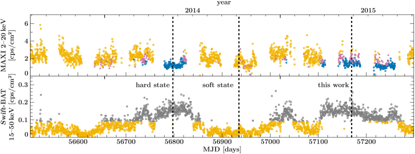
Figure 1.— MAXI light curve in the 2–20 keV band for Cyg X-1 and Swift/BAT light curve in the 15–50 keV band, both binned to 6 hours. For both instruments, yellow circles represent soft states, magenta triangles intermediate states and blue squares hard states. For the Swift/BAT light curve, gray circles indicate either hard or intermediate states that cannot be easily distinguished in the BAT energy range. The vertical lines mark the times of NuSTAR observations from this work, hard state (Parker et al., 2015; Basak et al., 2017) and soft state (Walton et al., 2016).

Figure 2.— (a) NuSTAR 3–79 keV light curve with FPMA and FPMB rates added together and (b) NuSTAR hardness ratio (10–79/3–10 keV) for Cyg X-1. The time bins are 50 s in duration.

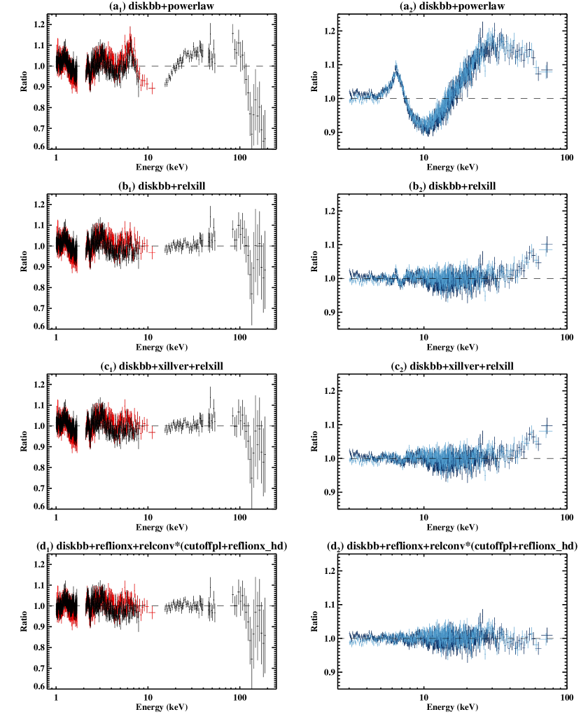
Figure 3.— Data-to-model ratio plots for the four models indicated above each plot. The Suzaku (left panels) and NuSTAR (right panels) spectra were fitted together, but the data-to-model ratios are shown separately for clarity. The left panels ($a_{1}$, $b_{1}$, $c_{1}$, and $d_{1}$) show the XIS data (red and black), the PIN data, and the GSO data at the highest energies. The right panels ($a_{2}$, $b_{2}$, $c_{2}$, and $d_{2}$) show FPMA (dark blue) and FPMB (light blue). The XIS and NuSTAR spectra are binned in XSPEC (only for visual clarity) to levels of 30-$\sigma$ per bin and 50-$\sigma$ per bin, respectively.

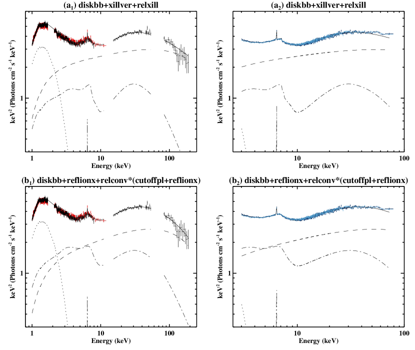
Figure 4.— Unfolded Suzaku (left panels) and NuSTAR (right panels) spectra fitted with two models with the iron abundance parameter free. In all panels, the components are diskbb (dotted line), cutoffpl (dashed line), and reflection component (dash-dotted line). Although a full reflionx model is also included, only the narrow iron line is visible. The solid line is the total of all the components. The residuals for panels $a_{1}$ and $a_{2}$ are shown in Figure 3c₁ and 3c₂. The XIS and NuSTAR spectra are binned in XSPEC (only for visual clarity) to levels of 30-$\sigma$ per bin and 50-$\sigma$ per bin, respectively.

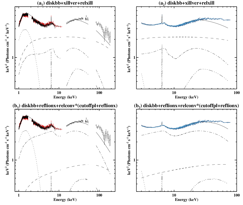
Figure 5.— Unfolded Suzaku (left panels) and NuSTAR (right panels) spectra fitted with two models with the iron abundance parameter fixed to $A_{\rm Fe}=1$. The components use the same line styles as in Figure 4, but the reflection hump for the reflionx model (triple-dot-dashed line) is visible because the the lower iron abundance forces the overall normalization of this component to increase. Although the only change in the model from the spectra shown in Figure 4 is the factor of $\sim$10 lower $A_{\rm Fe}$, the differences between the data and the model are largest at the high energy end of the spectrum.

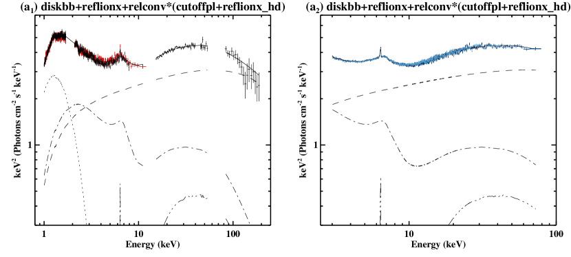
Figure 6.— Unfolded Suzaku (left panels) and NuSTAR (right panels) spectra fitted with a model that has solar abundances ($A_{\rm Fe}=1$), but with an electron density of $n_{e}=4\times 10^{20}$ cm^-3 (compared to $10^{15}$ cm^-3 for Figures 4 and 5). The reflection component (dash-dotted line) has a larger soft excess due to the higher electron density. The residuals are shown in Figure 3d₁ and 3d₂.

Figure 7.— Relativistic reflection models in the NuSTAR bandpass using the reflionx_hd model with values of the electron density ranging from $n_{e}=10^{15}$ to $4\times 10^{20}$ cm^-3. The highest density model is a component in the full spectrum.

Table 1Observing Log and Exposure Times

			Start Time (UT)	End Time (UT)	Livetime
Mission	Instrument	ObsID	(in 2015)	(in 2015)	(s)
NuSTAR	FPMA	30101022002	May 27, 17.3 h	May 28, 11.8 h	19,860
NuSTAR	FPMB	”	”	”	20,500
Suzaku	XIS0	410018010	May 27, 17.2 h	May 28, 15.6 h	1,098
Suzaku	XIS1	”	May 27, 16.7 h	May 28, 18.8 h	4,991
Suzaku	XIS3	”	May 27, 16.7 h	May 28, 15.1 h	2,913
Suzaku	HXD/PIN	”	May 27, 17.4 h	May 28, 18.1 h	18,620
Suzaku	HXD/GSO	”	”	”	18,620

Table 2Fit Parameters for Reflection Models with Free Iron Abundnace

Parameter	Unit/Description	Value	Valuea
		(relxill-based)	(reflionx-based)
Interstellar Absorption
$N_{\rm H}$	$10^{21}$ cm-2	6.0	6.0b
Disk-blackbody
$kT_{\rm in}$	keV	$0.378\pm 0.002$	$0.376\pm 0.002$
$N_{\rm DBB}$	Normalization	$44,600\pm 1100$	$46,600^{+1500}_{-1400}$
Direct component plus partially ionized/relativistic reflection
$\Gamma$	Photon Index	$1.826\pm 0.004$	$1.712\pm 0.006$
$E_{\rm cut}$	keV	300b	300b
$\log{\xi}$	$\xi$ in erg cm s-1	$3.374\pm 0.013$	$3.588^{+0.044}_{-0.035}$
$A_{\rm Fe}$	Abundance relative to solar	$>$9.96	$10.6^{+1.6}_{-0.9}$
$\Omega/2\pi$	Covering fraction	$0.87\pm 0.04$	—
$q_{\rm in}$	Emissivity Index	$9.1^{+0.5}_{-0.4}$	$9.3\pm 0.3$
$q_{\rm out}$	Emissivity Index	3b	3b
$R_{\rm break}$	Index Break Radius ($R_{\rm ISCO}$)	$2.24^{+0.07}_{-0.22}$	$2.41^{+0.06}_{-0.22}$
$R_{\rm in}$	Disk Inner Radius ($R_{\rm ISCO}$)	$1.33^{+0.03}_{-0.06}$	$1.26^{+0.03}_{-0.02}$
$R_{\rm out}$	Outer Radius for Reflection ($R_{\rm g}$)	400b	400b
$a_{*}$	Black Hole Spin	$>$0.987	$>$0.988
$i$	Inclination (∘)	$37.5\pm 0.7$	$35.6\pm 1.0$
$N_{\rm relxill}$	Normalization	$(3.74^{+0.04}_{-0.05})\times 10^{-2}$	—
$N_{\rm reflionx}$	Normalization	—	$(1.88^{+0.13}_{-0.15})\times 10^{-4}$
$N_{\rm cutoffpl}$	Normalization	—	$26.2^{+0.7}_{-1.3}$
Neutral reflection
$\log{\xi}$	$\xi$ in erg cm s-1	0.0b	1.0b
$N_{\rm xillver}$	Normalization	$(1.77^{+0.22}_{-0.25})\times 10^{-3}$	—
$N_{\rm reflionx}$	Normalization	—	$(3.5\pm 0.4)\times 10^{-4}$
Cross-Normalization Constants (relative to XIS0+XIS3)
$C_{\rm XIS1}$	–	$0.794\pm 0.003$	$0.794\pm 0.003$
$C_{\rm FPMA}$	–	$1.005\pm 0.004$	$1.002\pm 0.004$
$C_{\rm FPMB}$	–	$1.007\pm 0.004$	$1.003\pm 0.004$
$C_{\rm PIN}$	–	$1.247\pm 0.007$	$1.244\pm 0.007$
$C_{\rm GSO}$	–	$1.13\pm 0.03$	$1.15\pm 0.03$
Goodness of fit
$\chi^{2}/\nu$	–	3566/2750	3360/2750

Table 3Fit Parameters for High Density Reflection Model

Parameter	Unit/Description	Value	Valuea
		(power-law emissivity)	(lamppost)
Interstellar Absorption
$N_{\rm H}$	$10^{21}$ cm-2	6.0	6.0b
Disk-blackbody
$kT_{\rm in}$	keV	$0.317\pm 0.002$	$0.317\pm 0.002$
$N_{\rm DBB}$	Normalization	$100,500^{+3700}_{-3500}$	$100,400^{+2500}_{-3400}$
Direct component plus partially ionized/relativistic reflection
$\Gamma$	Photon Index	$1.779\pm 0.007$	$1.777^{+0.009}_{-0.006}$
$E_{\rm cut}$	keV	300b	300b
$\log{\xi}$	$\xi$ in erg cm s-1	$3.302^{+0.011}_{-0.006}$	$3.303^{+0.014}_{-0.002}$
$A_{\rm Fe}$	Abundance relative to solar	1.0	1.0c
$q_{\rm in}$	Emissivity Index	3b	—
$q_{\rm out}$	Emissivity Index	3b	—
$h$	Lamppost height ($R_{\rm ISCO}$)	—	$20.0^{+15.9}_{-1.0}$
$R_{\rm in}$	Disk Inner Radius ($R_{\rm ISCO}$)	$7.3^{+4.6}_{-1.9}$	$2.9^{+3.5}_{-0.8}$
$R_{\rm out}$	Outer Radius for Reflection ($R_{\rm g}$)	400b	400b
$a_{*}$	Black Hole Spin	$>$0.93	$0.949^{+0.013}_{-0.019}$
$i$	Inclination (∘)	$18^{+4}_{-5}$	$<$20
$n_{e}$	Density in $10^{20}$ cm-3	$3.98^{+0.12}_{-0.25}$	$3.98^{+0.13}_{-0.33}$
$N_{\rm reflionx}$	Normalization	$97.9^{+2.9}_{-1.5}$	$97.8^{+4.0}_{-1.5}$
$N_{\rm cutoffpl}$	Normalization	$24.8\pm 0.4$	$24.8^{+0.4}_{-0.3}$
Neutral reflection
$\log{\xi}$	$\xi$ in erg cm s-1	1.0b	1.0b
$N_{\rm reflionx}$	Normalization	$(8.6\pm 0.8)\times 10^{-4}$	$(8.3^{+0.2}_{-0.7})\times 10^{-4}$
Cross-Normalization Constants (relative to XIS0+XIS3)
$C_{\rm XIS1}$	–	$0.793\pm 0.003$	$0.793^{+0.001}_{-0.003}$
$C_{\rm FPMA}$	–	$1.002\pm 0.004$	$1.002^{+0.004}_{-0.001}$
$C_{\rm FPMB}$	–	$1.004\pm 0.004$	$1.004^{+0.004}_{-0.001}$
$C_{\rm PIN}$	–	$1.244\pm 0.007$	$1.244\pm 0.007$
$C_{\rm GSO}$	–	$1.02\pm 0.03$	$1.02\pm 0.03$
Goodness of fit
$\chi^{2}/\nu$	–	3020/2752	3016/2751

Table 4Key Parameters for Cyg X-1 in different Spectral States

	Tomsick et al. (2014)	Walton et al. (2016)	This work	This work	Basak et al. (2017)
	(NuSTAR and	(4 NuSTAR	relxill	reflionx_hd	(NuSTAR and
	Suzaku)	observations)		(lamppost)	Suzaku)
Spectral State	soft	soft	intermediate	intermediate	hard
$kT_{\rm in}$ (keV)	0.56	0.40–0.47	$0.378\pm 0.002$	$0.317\pm 0.002$	0.14–0.15
$\Gamma$	2.6–2.7	2.56–2.74	$1.826\pm 0.004$	$1.777^{+0.009}_{-0.006}$	1.70–1.71
$R_{\rm in}/R_{\rm ISCO}$	1	1	$1.33^{+0.03}_{-0.06}$	$2.9^{+3.5}_{-0.8}$	13–20 $R_{g}$
$a_{*}$	$>$0.83	0.93–0.96	$>$0.987	$0.949^{+0.013}_{-0.019}$	—
$i$ (∘)	$>$40	38.2–40.8	$37.5\pm 0.7$	$<$20	24–43
$A_{\rm Fe}$	1.9–2.9	4.0–4.3	$>$9.96	1.0	2.2–4.6
Flux	$8.0\times 10^{-8}$	—	$4.4\times 10^{-8}$	—	$2.9\times 10^{-8}$
Luminosity	$3.3\times 10^{37}$	—c	$1.8\times 10^{37}$	—d	$1.2\times 10^{37}$
$L/L_{\rm Edd}$	1.72%	—c	0.94%	—d	0.62%

References

- Bardeen & Petterson (1975) Bardeen, J. M., & Petterson, J. A., 1975, ApJ, 195, L65
- Basak et al. (2017) Basak, R., Zdziarski, A. A., Parker, M., & Islam, N., 2017, MNRAS, 472, 4220
- Dauser et al. (2013) Dauser, T., Garcia, J., Wilms, J., Böck, M., Brenneman, L. W., Falanga, M., Fukumura, K., & Reynolds, C. S., 2013, MNRAS, 430, 1694
- Duro et al. (2011) Duro, R., et al., 2011, A&A, 533, L3
- Fabian et al. (2013) Fabian, A. C., et al., 2013, MNRAS, 429, 2917
- Fabian et al. (1989) Fabian, A. C., Rees, M. J., Stella, L., & White, N. E., 1989, MNRAS, 238, 729
- Fabian et al. (2012) Fabian, A. C., et al., 2012, MNRAS, 424, 217
- Fabian et al. (2009) Fabian, A. C., et al., 2009, Nature, 459, 540
- Fragile et al. (2007) Fragile, P. C., Blaes, O. M., Anninos, P., & Salmonson, J. D., 2007, ApJ, 668, 417
- Fürst et al. (2015) Fürst, F., et al., 2015, ApJ, 808, 122
- García et al. (2014) García, J., et al., 2014, ApJ, 782, 76
- García et al. (2013) García, J., Dauser, T., Reynolds, C. S., Kallman, T. R., McClintock, J. E., Wilms, J., & Eikmann, W., 2013, ApJ, 768, 146
- García, Kallman & Mushotzky (2011) García, J., Kallman, T. R., & Mushotzky, R. F., 2011, ApJ, 731, 131
- García et al. (2016) García, J. A., Fabian, A. C., Kallman, T. R., Dauser, T., Parker, M. L., McClintock, J. E., Steiner, J. F., & Wilms, J., 2016, MNRAS, 462, 751
- García et al. (2015) García, J. A., Steiner, J. F., McClintock, J. E., Remillard, R. A., Grinberg, V., & Dauser, T., 2015, ApJ, 813, 84
- Gies & Bolton (1986) Gies, D. R., & Bolton, C. T., 1986, ApJ, 304, 371
- Gou et al. (2014) Gou, L., et al., 2014, ApJ, 790, 29
- Grinberg et al. (2013) Grinberg, V., et al., 2013, A&A, 554, A88
- Gruber et al. (1999) Gruber, D. E., Matteson, J. L., Peterson, L. E., & Jung, G. V., 1999, ApJ, 520, 124
- Harrison et al. (2013) Harrison, F. A., et al., 2013, ApJ, 770, 103
- Jourdain et al. (2012) Jourdain, E., Roques, J. P., Chauvin, M., & Clark, D. J., 2012, ApJ, 761, 27
- Kouzu et al. (2013) Kouzu, T., et al., 2013, PASJ, 65, 74
- Koyama et al. (2007) Koyama, K., et al., 2007, PASJ, 59, 23
- Krimm et al. (2013) Krimm, H. A., et al., 2013, ApJS, 209, 14
- Laurent et al. (2011) Laurent, P., Rodriguez, J., Wilms, J., Cadolle Bel, M., Pottschmidt, K., & Grinberg, V., 2011, Science, 332, 438
- Lightman & White (1988) Lightman, A. P., & White, T. R., 1988, ApJ, 335, 57
- Matsuoka et al. (2009) Matsuoka, M., et al., 2009, PASJ, 61, 999
- McConnell et al. (2002) McConnell, M. L., et al., 2002, ApJ, 572, 984
- Meyer, Liu & Meyer-Hofmeister (2000) Meyer, F., Liu, B. F., & Meyer-Hofmeister, E., 2000, A&A, 361, 175
- Miller et al. (2002) Miller, J. M., et al., 2002, ApJ, 578, 348
- Miller et al. (2012) Miller, J. M., Pooley, G. G., Fabian, A. C., Nowak, M. A., Reis, R. C., Cackett, E. M., Pottschmidt, K., & Wilms, J., 2012, ApJ, 757, 11
- Miller et al. (2015) Miller, J. M., et al., 2015, ApJ, 799, L6
- Mitsuda et al. (2007) Mitsuda, K., et al., 2007, PASJ, 59, 1
- Mitsuda et al. (1984) Mitsuda, K., et al., 1984, PASJ, 36, 741
- Nowak et al. (2011) Nowak, M. A., et al., 2011, ApJ, 728, 13
- Orosz et al. (2011) Orosz, J. A., McClintock, J. E., Aufdenberg, J. P., Remillard, R. A., Reid, M. J., Narayan, R., & Gou, L., 2011, ApJ, 742, 84
- Parker et al. (2016) Parker, M. L., et al., 2016, ApJ, 821, L6
- Parker et al. (2015) Parker, M. L., et al., 2015, ApJ, 808, 9
- Reid et al. (2011) Reid, M. J., McClintock, J. E., Narayan, R., Gou, L., Remillard, R. A., & Orosz, J. A., 2011, ApJ, 742, 83
- Reynolds et al. (2012) Reynolds, C. S., Brenneman, L. W., Lohfink, A. M., Trippe, M. L., Miller, J. M., Fabian, A. C., & Nowak, M. A., 2012, ApJ, 755, 88
- Risaliti et al. (2013) Risaliti, G., et al., 2013, Nature, 494, 449
- Ross & Fabian (2005) Ross, R. R., & Fabian, A. C., 2005, MNRAS, 358, 211
- Ross & Fabian (2007) Ross, R. R., & Fabian, A. C., 2007, MNRAS, 381, 1697
- Schandl & Meyer (1994) Schandl, S., & Meyer, F., 1994, A&A, 289, 149
- Steiner et al. (2010) Steiner, J. F., McClintock, J. E., Remillard, R. A., Gou, L., Yamada, S., & Narayan, R., 2010, ApJ, 718, L117
- Stirling et al. (2001) Stirling, A. M., Spencer, R. E., de la Force, C. J., Garrett, M. A., Fender, R. P., & Ogley, R. N., 2001, MNRAS, 327, 1273
- Svensson & Zdziarski (1994) Svensson, R., & Zdziarski, A. A., 1994, ApJ, 436, 599
- Takahashi et al. (2007) Takahashi, T., et al., 2007, PASJ, 59, 35
- Tananbaum et al. (1972) Tananbaum, H., Gursky, H., Kellogg, E., Giacconi, R., & Jones, C., 1972, ApJ, 177, L5
- Tomsick et al. (2014) Tomsick, J. A., et al., 2014, ApJ, 780, 78
- Tomsick et al. (2009) Tomsick, J. A., Yamaoka, K., Corbel, S., Kaaret, P., Kalemci, E., & Migliari, S., 2009, ApJ, 707, L87
- Torii et al. (2011) Torii, S., et al., 2011, PASJ, 63, S771
- Verner et al. (1996) Verner, D. A., Ferland, G. J., Korista, K. T., & Yakovlev, D. G., 1996, ApJ, 465, 487
- Walton et al. (2017) Walton, D. J., et al., 2017, ApJ, 839, 110
- Walton et al. (2016) Walton, D. J., et al., 2016, ApJ, 826, 87
- Wang et al. (2012) Wang, H., Zhou, H., Yuan, W., & Wang, T., 2012, ApJ, 751, L23
- Wilms, Allen & McCray (2000) Wilms, J., Allen, A., & McCray, R., 2000, ApJ, 542, 914
- Xiang et al. (2011) Xiang, J., Lee, J. C., Nowak, M. A., & Wilms, J., 2011, ApJ, 738, 78
- Yamada et al. (2013) Yamada, S., Makishima, K., Done, C., Torii, S., Noda, H., & Sakurai, S., 2013, PASJ, 65, 80
- Zoghbi et al. (2016) Zoghbi, A., et al., 2016, ApJ, 833, 165