Cooling by heating in nonequilibrium nanosystems

Abstract

We demonstrate the possiblity to cool nanoelectronic systems in nonequilibrium situations by increasing the temperature of the environment. Such cooling by heating is possible for a variety of experimental conditions where the relevant transport-induced excitation processes become quenched and deexcitation processes are enhanced upon an increase of temperature. The phenomenon turns out to be robust with respect to all relevant parameters. It is especially pronounced for higher bias voltages and weak to moderate coupling. Our findings have implications for open quantum systems in general, where electron transport is coupled to mechanical (phononic) or photonic degrees of freedom. In particular, molecular junctions with rigid tunneling pathways or quantum dot circuit QED systems meet the required conditions.

Nanoelectronic systems exhibit a plethora of fundamentally interesting physical properties and, at the same time, are considered as promising architectures for technological applications, ranging from transistor Piva et al. (2005); Song et al. (2009) to quantum information devices Loss and DiVincenzo (1998); Petersson et al. (2011). Experimental realizations include single-molecule junctions Reed et al. (1997); Reichert et al. (2002); Park et al. (2002); Reed (2004); Wu et al. (2004); Cuniberti et al. (2005); Venkataraman et al. (2006); Secker et al. (2011); Cuevas and Scheer (2010), atomic wires Agrait et al. (2002, 2003); Schäfer et al. (2009); Blumenstein et al. (2011), carbon nanotube LeRoy et al. (2004); Tans et al. (1997); Sapmaz et al. (2005, 2006); Leturcq et al. (2009); Delbecq et al. (2011, 2013) and semiconductor based quantum dot systems Reed et al. (1988); van Wees et al. (1988); Holleitner et al. (2001); van der Wiel et al. (2002); Ihn et al. (2007); Kießlich et al. (2007); Tutuc et al. (2011); Liu et al. (2014); Beckel et al. (2014). A limiting factor is current-induced heating associated with the excitation of mechanical or electromagnetic degrees of freedom. Such heating limits the control, coherence or even the mechanical stability of these devices. It is therefore expedient to identify and understand the intrinsic cooling mechanisms of nanoelectronic systems.

(a) transport	(b) transport	(c) pair-creation

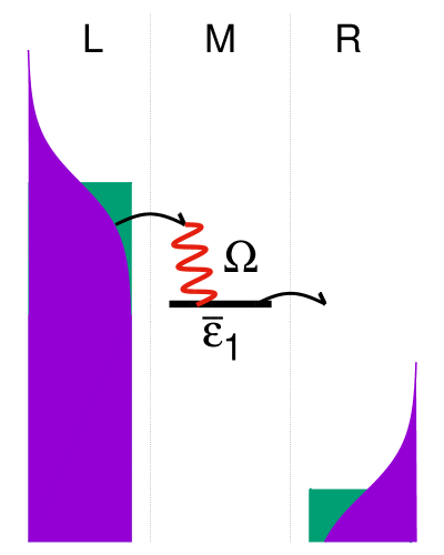
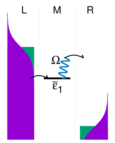
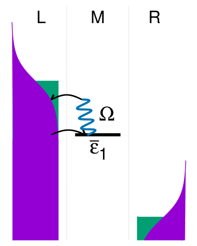
Figure 1: Sketch of representative inelastic processes in a biased molecular junction, where electrons tunnel in two, sequential resonant tunneling processes onto and off the molecule (M). The green and purple areas represent occupied states in the left (L) and right lead (R) for lower and higher temperatures, respectively. Panel (a) and (b) depict transport processes, where the vibrational mode is excited and deexcited upon tunneling of an electron from L to M and from M to R, respectively. At low temperatures, process (a) requires higher bias voltages, $\Phi\gtrsim 2(\overline{\epsilon}_{1}+\Omega)$ than process (b), $\Phi\gtrsim 2\overline{\epsilon}_{1}$. At these voltages, an increase of temperature reduces the initial state population of both processes. Panel (c) depicts a pair-creation process, where the electron returns to the original electrode. For $\Phi\gtrsim 2(\overline{\epsilon}_{1}+\Omega)$ and low temperatures, this deexcitation process is Pauli-blocked since its final state population is almost $1$. It can be reactivated by an increase of temperature which reduces the final state population.

Nonequilibrium steady states offer the possibility for unprecedented control or cooling strategies. One possibility is to use the bias voltage which is applied to the device. In many situations, a non-zero voltage leads to additional heating processes and higher levels of excitation. However, in the presence of co-tunneling assisted sequential tunneling Lüffe et al. (2008); Hüttel et al. (2009), higher-lying electronic states Härtle et al. (2009); Romano et al. (2010), antiresonances McEniry et al. (2009), suitably defined spectral properties of the leads Galperin et al. (2009); Gelbwaser-Klimovsky et al. (2017), donor-acceptor structures Galperin et al. (2009); Lü et al. (2011); Simine and Segal (2012) or electron-electron interactions Härtle and Thoss (2011a), an increase in voltage can lead to lower excitation levels of the mechanical or photonic degrees of freedom. Another possibility is to use spin-polarized currents Brüggemann et al. (2014).

In this work, we demonstrate how an increase of the environments temperature leads to lower excitation levels of the nanoelectronic system and thus stabilizes the device. To be specific, we consider models of single-molecule junctions in the following. The principle, however, applies to any few-level systems where electron transport is coupled to mechanical or, e.g. in the case of cavity QED systems Delbecq et al. (2011, 2013); Liu et al. (2014), photonic degrees of freedom. It is emphasized that our scheme for cooling by heating does not involve heat or temperature gradients such as in domestic Gordon and Ng (2000) or quantum absorption refrigerators Palao et al. (2001); Linden et al. (2010); Levy and Kosloff (2012); Cleuren et al. (2012); Gelbwaser-Klimovsky and Kurizki (2014); Gelbwaser-Klimovsky et al. (2015) or optomechanical devices Mari and Eisert (2012). Rather, chemical potential differences induced by an external bias voltage lead to transport through the nanosystem between two Fermion reservoirs where heating the reservoirs cools down the nanosystem.

The phenomenon of thermal stabilization predicted here is most strongly pronounced in the regime of weak to moderate molecule-lead and electronic-vibrational/photonic coupling and high enough (but still practically relevant) voltages, where transport-induced heating mechanisms (cf. Fig. 1a) are quenched for higher temperatures and, at the same time, cooling mechanisms are either less affected (cf. Fig. 1b) or become enhanced (cf. Fig. 1c). An important characteristics of this regime is that weaker coupling to vibrational or photonic degrees of freedom results in higher excitation levels Mitra et al. (2004); Koch et al. (2006); Avriller (2011); Härtle and Thoss (2011a, b); Kast et al. (2011); Härtle and Kulkarni (2015). In the limit of vanishing couplings and temperatures, this leads to an indefinite increase of the excitation level for harmonic modes Härtle and Thoss (2011b); Härtle and Kulkarni (2015), that is a vibrational instability .

We consider transport through a molecule (M) that is coupled to a left (L) and a right electrode (R). We describe this transport setup by the Hamiltonian $H=H_{\text{M}}+H_{\text{ME}}+H_{\text{E}}$ where (using units where $\hbar=1$ and $k_{\text{B}}=1$)

$$H_{\text{M}} = \sum_{m\in\text{M}}\epsilon_{m}d_{m}^{\dagger}d_{m}+\sum_{m<n\in\text{M}}U_{mn}d_{m}^{\dagger}d_{m}d_{n}^{\dagger}d_{n}$$

$$+H_{\text{Vib}}+\sum_{m\in\text{M}}\lambda_{m}(a+a^{\dagger})d_{m}^{\dagger}d_{m},$$

$$H_{\text{Vib}} = \Omega a^{\dagger}a+\sum_{\xi}V_{\xi}(a+a^{\dagger})^{\xi},$$ (2)

$$H_{\text{E}} = \sum_{k\in\text{L,R}}\epsilon_{k}c_{k}^{\dagger}c_{k}+\sum_{\alpha}\omega_{\alpha}b_{\alpha}^{\dagger}b_{\alpha},$$ (3)

$$H_{\text{ME}} = \sum_{m\in\text{M},k\in\text{L,R}}(V_{mk}c^{\dagger}_{k}d_{m}+V_{mk}^{*}d_{m}^{\dagger}c_{k})$$

$$+\sum_{\alpha}W_{\alpha}(a+a^{\dagger})(b_{\alpha}+b_{\alpha}^{\dagger}).$$

It includes a discrete set of electronic eigenstates with energies $\epsilon_{m}$ and density-density interactions $U_{mn}$ between electrons in states $m$ and $n$. The states of the molecule are coupled to a continuum of electronic states with energies $\epsilon_{k}$ and coupling matrix elements $V_{mk}$ in the left (L) and the right (R) electrode. The corresponding tunneling efficiency or hybridization function is $\Gamma_{K,mn}(\epsilon)=2\pi\sum_{k\in K}V_{mk}^{*}V_{nk}\delta(\epsilon-\epsilon_{k})$ ($K\in\{\text{L,R}\}$). Throughout this work, we use the wide-band approximation $\Gamma_{K,mn}(\epsilon)\approx\Gamma_{K,mn}$ and consider a symmetric drop of the applied bias voltage, i.e. the chemical potentials in the left and right lead are given by $\mu_{\text{L/R}}=\pm\Phi/2$. We model vibrational effects by the vibrational Hamiltonian $H_{\text{Vib}}$, which, for $V_{\xi}=0$, is harmonic with frequency $\Omega$ and, for non-zero $V_{\xi}$, includes generic anharmonic effects, most importantly a non-equidistant energy spectrum. The mode may be representative of the dominant reaction coordinate of the molecule. It is coupled to the electronic states of the molecule by coupling strengths $\lambda_{m}$ and a bath of harmonic oscillators $\alpha$ with coupling strengths $W_{\alpha}$ in order to account for intramolecular vibrational energy redistribution Mukamel and Smalley (1980); Freed and Nitzan (1983); Zewail (1994); Nesbitt and Field (1996) or energy losses to a bosonic junction’s environment Tao (2006); Jorn and Seidemann (2009). Note that we use the same temperature $T$ to describe the bath and the electrodes, that is we do not consider any external temperature gradients.

We solve the above transport problem using the well established Born-Markov (BM) May (2002); Mitra et al. (2004); Lehmann et al. (2004); Harbola et al. (2006); Volkovich et al. (2008); Härtle et al. (2009); Härtle and Thoss (2011a); Pshenichnyuk and Čížek (2011) and the recently developed hierarchical quantum master equation (HQME) approach Schinabeck et al. (2016). Explicit formulas and detailed derivations for HQME and BM can be found in Refs. Jin et al. (2008); Schinabeck et al. (2016) and Härtle and Thoss (2011a, b), respectively. The central quantity of both approaches is the reduced density matrix $\sigma$ of the molecule which includes the electronic levels and the vibrational mode. We determine it as the stationary solution of its equation of motion,

$$0\,\stackrel{{\scriptstyle!}}{{=}}\,\frac{\partial\sigma(t)}{\partial t}\,=\,-i\left[H_{\text{M}},\sigma(t)\right]-\sigma^{(1)}(t),$$ (5)

where the first term of the rhs describes the internal dynamics of the molecule and the second term $\sigma^{(1)}(t)$ the influence of the environment. Using HQME, we determine $\sigma^{(1)}(t)$ by solving its equation of motion, which leads to second- and, consequently, higher-tier operators $\sigma^{(n)}(t)$ with $n>1$. Truncation of this hierarchy corresponds to a truncated hybridization expansion. HQME thus allows us to systematically assess the importance of higher-order effects. The basic effect, however, is already included in BM, where the first-tier operator

$$\sigma^{(1)}(t) = \int_{0}^{\infty}\text{d}\tau\,\text{tr}_{\text{E}}\{\left[H_{\text{ME}},\left[H_{\text{ME}}(\tau),\sigma(t)\sigma_{\text{E}}\right]\right]\}$$ (6)

is expressed in terms of the reduced density matrix $\sigma(t)$, the density matrix of the environment $\sigma_{\text{E}}$ and the coupling operator $H_{\text{ME}}(\tau)=\text{e}^{-i(H_{\text{M}}+H_{\text{E}})\tau}H_{\text{ME}}\text{e}^{i(H_{\text{M}}+H_{\text{E}})\tau}$. Thus, BM corresponds to a first-tier truncation of HQME, including the Markov approximation $\sigma(t-\tau)\approx\text{e}^{iH_{\text{M}}\tau}\sigma(t)\text{e}^{-iH_{\text{M}}\tau}$ which enters the above integral kernel. In addition, we disregard off-diagonal elements of the density matrix and renormalization effects. A discussion on the role of vibrational off-diagonal elements can be found, for example, in Ref. Härtle and Thoss (2011a). The role of renormalization effects in the presence of electron-electron interactions has been outlined in Refs. König and Martinek (2003); Wunsch et al. (2005); Härtle and Millis (2014), including a pronounced resonance in the conductance-voltage characteristics Härtle et al. (2013); Hell et al. (2015); Wenderoth et al. (2016). These effects, however, are not important for our discussion, which we show explicitly by a comparison to HQME where both off-diagonal elements and renormalization effects are included.

We introduce the phenomenon of thermal stabilization for a minimal model first. It includes a single electronic state with the polaron-shifted energy $\overline{\epsilon}_{1}\equiv\epsilon_{1}-\lambda_{1}^{2}/\Omega=3\Omega$ that is weakly coupled to an undamped ($W_{\alpha}=0$) harmonic mode with $\lambda_{1}=\Omega/10$ and the leads with $\Gamma_{\text{L/R},11}=\Omega/1000\equiv\Gamma_{\text{L/R}}$. We measure the stability of the junction by the average vibrational energy $\langle H_{\text{Vib}}\rangle$. It is the result of thermal excitations, transport-induced excitation processes (Figs. 1a) and deexcitation processes which are associated either with transport (Fig. 1b) or pair-creation processes (Fig. 1c). High values indicate a less stable junction, low ones a more stable junction.

The average vibrational energy $\langle H_{\text{Vib}}\rangle$ of our minimal model is shown in Fig. 2a as a function of both bias voltage $\Phi$ and temperature $T$. At very low temperatures, $T\rightarrow 0$, we observe a step-like increase with bias voltages. The steps at $\Phi=2(\overline{\epsilon}_{1}+\Omega)=8\Omega$, $10\Omega$, $12\Omega$ … correspond to the opening of transport-induced heating processes (see Fig. 1a) and the closing of cooling processes via pair creation (see Fig. 1c), which are associated with single, two, three … phonon transitions, respectively. Increasing the temperature, the steps are smeared out and the vibrational energy decreases due to suppression (enhancement) of heating (cooling) rates as explained below.

We study this temperature effect more closely in Fig. 2b which shows the vibrational energy as a function of temperature for different fixed values of the applied bias voltage $\Phi$. For low voltages $\Phi\lesssim 2(\overline{\epsilon}_{1}+\Omega)$ (dashed grey line), the vibrational energy increases monotonically with temperature, starting from low transport-induced values which evolve towards values that are given by a thermal distribution (cf. the blue line which depicts the Bose function $1/(\text{exp}(\Omega/T)-1))$). The vibrational energy is relatively low in this regime because transport-induced heating is outbalanced by both transport-induced cooling (Fig. 1b) and pair-creation processes (Fig. 1c) Härtle and Thoss (2011a). Additional heating processes (Fig. 1a) become active at higher bias voltages $\Phi\gtrsim 2(\overline{\epsilon}_{1}+\Omega)$, while, in parallel, pair-creation processes with a single phonon transition become blocked (e.g. the one depicted in Fig. 1c). Thus, the transport-induced vibrational energy increases significantly at these voltages (cf. solid and dashed green lines). This leads to a qualitatively different temperature dependence, in particular a negative slope in an intermediate temperature regime, which becomes more pronounced for higher bias voltages. This is the regime where thermal stabilization occurs, that is a decrease of the vibrational energy as the temperature of the environment is increased. The mechanism can be rationalized by the effect of thermal broadening which quenches preferentially the additional heating processes (compare Fig. 1a to Fig. 1b) and allows pair-creation processes (Fig. 1c) to cool the junction again before thermal fluctuations override any transport-induced effects. For very low temperatures, $T\ll\Omega/2$, these broadening effects are too inefficient, as reflected by the plateau which appears before the average vibrational energy decreases. The small peak in the green line indicates the onset of transport-induced excitation processes (Fig. 1a) and the suppression of pair creation processes (Fig. 1c) with two vibrational quanta which, for $\Phi=9.5\Omega$, occurs before pair-creation processes with a single vibrational quantum become re-activated.

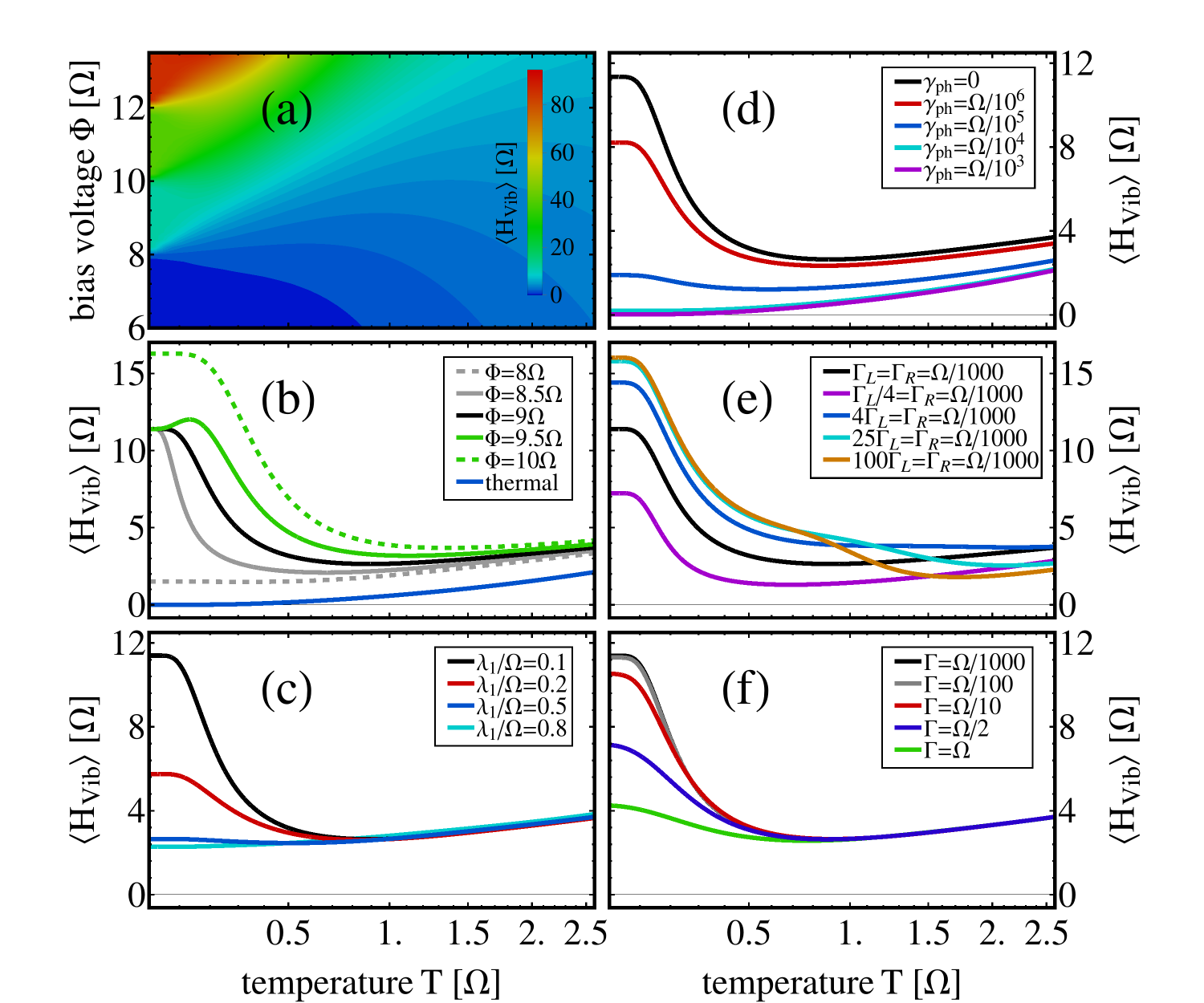
Figure 2: Average vibrational energy $\langle H_{\text{Vib}}\rangle$ for our model of a molecular junction as a function of both temperature and applied bias voltage $\Phi$ (Panel (a)), as a function of temperature for fixed voltages (Panel (b)), different electronic-vibrational coupling strengths $\lambda$ (Panel (c)), mode-bath couplings (Panel (d)), molecule-lead coupling ratios $\Gamma_{\text{L}}/\Gamma_{\text{R}}$ (Panel (e)) and strengths $\Gamma$ (Panel (f)). For the results shown in Panels (c)–(f), we used $\Phi=9\Omega$. If not stated otherwise, the other parameters are $\overline{\epsilon}_{1}=3\Omega$, $\lambda_{1}=\Omega/10$, $\Gamma_{\text{L}}=\Gamma_{\text{R}}=\Omega/1000$ and $\gamma_{\text{ph}}=2\pi\sum_{\alpha}|W_{\alpha}|^{2}\delta(\Omega-\omega_{\alpha})$. The results shown in Panels (a)–(e) and (f) have been obtained using BM and HQME, respectively.

As will be shown below, the phenomenon of thermal stabilization is robust. Nevertheless, the extent of the regime where thermal stabilization occurs depends on the specific junction parameters which we now study one by one. To this end, we point out that the phenomenon occurs in the same regime of bias voltages, $\Phi\gtrsim 2(\overline{\epsilon}_{1}+\Omega)$, where the model exhibits a vibrational instability as $\lambda,T,\Gamma_{\text{L/R}}\rightarrow 0$, that is an indefinite increase of vibrational energy as the electronic-vibrational coupling constant is decreased Mitra et al. (2004); Koch et al. (2006); Avriller (2011); Kast et al. (2011); Härtle and Thoss (2011b); Härtle and Kulkarni (2015). Consequently, the transport-induced vibrational energy is higher and the stabilization effect is more pronounced for weaker electronic-vibrational coupling, as can be seen in Fig. 2c, where we show the temperature dependence of the vibrational energy for different electronic-vibrational coupling strengths. While the vibrational energy of the mode is indeed lower for stronger coupling strengths, a negative slope can still be seen for intermediate coupling strengths, i.e. $\lambda/\Omega\lesssim 0.5$.

Another parameter of the model is the energy of the electronic level with respect to the Fermi level of the junction. Thermal stabilization, however, turns out to be rather insensitive to this parameter, unless additional pair-creation processes, e.g. with respect to the electrode with the lower chemical potential, come into play (see SI). The same is true, when additional electronic states are included, even in the presence of electron-electron interactions (cf. SI).

At this point, we increase the complexity of our model by coupling the vibrational mode to a heat bath. Fig. 2d shows the average vibrational energy $\langle H_{\text{Vib}}\rangle$ of the extended model as a function of temperature for different mode-bath coupling strengths. The overall effect of the bath is to reduce the vibrational energy and, consequently, to narrow the range of temperatures where an increase in temperature leads to a reduction of the vibrational energy. Nevertheless, thermal stabilization is observed also in the presence of coupling to a heat bath.

So far, we considered symmetric coupling to the leads. Thus, the rate of transport and pair-creation processes differ only by thermal factors. Asymmetric molecule-lead coupling, $\Gamma_{\text{L}}\neq\Gamma_{\text{R}}$, affects the balance between transport and pair-creation processes, leading, for example, to vibrational rectification Härtle and Thoss (2011a) or mode-selective vibrational excitation Härtle et al. (2010); Volkovich et al. (2011). Fig. 2e shows the average vibrational energy for our minimal model of a molecular junction as a function of temperature for different asymmetry scenarios. If the lead with the higher chemical potential is more strongly coupled to the molecule, cooling via pair-creation processes is more effective. The corresponding reduction of vibrational energy has a similar effect as coupling of the mode to a heat bath. In the opposite case, where the lead with the higher chemical potential is less strongly coupled to the molecule, cooling via pair-creation processes is less effective. Consequently, the average vibrational energy at low temperatures increases and the stabilization regime extends over a broader range of temperatures. In this regime, the quenching of heating processes is the dominant mechanism for thermal stabilization, in particular for $\Gamma_{\text{L}}\lesssim\Gamma_{\text{R}}/100$.

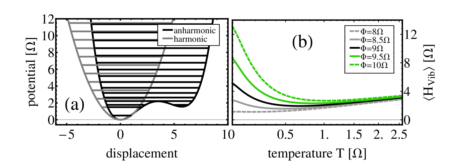
Figure 3: Panel (a): Potential of the vibrational motion for $V_{2}=0.136\Omega$, $V_{3}=0.084\Omega$ and $V_{4}=0.005\Omega$. Panel (b): Average vibrational energy $\langle H_{\text{Vib}}\rangle$ as a function of temperature for $\epsilon_{1}=3\Omega$ and the anharmonic potential shown in Panel (a). We used BM to obtain these results.

Next, we discuss the effect of higher-order processes and broadening due to the hybridization of the molecule with the leads. To this end, we employ the HQME approach and symmetric coupling to the leads ($\Gamma_{\text{L}}=\Gamma_{\text{R}}=\Gamma$). Fig. 2f shows converged data for the average vibrational energy as a function of temperature for different molecule-lead coupling strengths. In the anti-adiabatic regime $\Gamma\ll\Omega$ (black line), we recover the BM results. Increasing the coupling strength, the average vibrational energy at low temperatures decreases. We attribute this behavior to broadening effects due to the hybridization of the molecule with the leads which have a similar effect as an increased thermal broadening. Accordingly, the stabilization effect is most pronounced in the anti-adiabatic regime, where BM theory applies.

Last but not least, we demonstrate that the phenomenon of thermal stabilization is not restricted to harmonic vibrations. To this end, we relax the harmonic approximation and consider an anharmonic potential (see black line in Fig. 3a). The corresponding average vibrational energy is depicted in Fig. 3b. Despite differences to the harmonic case, the anharmonic system still exhibits a pronounced regime where thermal stabilization occurs. Qualitative changes occur at low temperatures, because transport-induced and pair-creation processes can now take place at a variety of energies, redistributing the onset voltages for excitation and deexcitation processes. Thus, e.g., the plateau at low temperatures ($T\ll\Omega$) is less pronounced.

We conclude that molecular junctions exhibit a broad range of parameters where they can be stabilized by increasing the temperature of the environment. As we showed, the stabilization effect is robust and occurs in the weak- to intermediate-coupling regime at voltages where resonant pair-creation processes with a single or more vibrational quanta (cf. Fig. 1c) are suppressed. This suppression is typical for low temperatures, i.e. $T\lesssim\Omega$. An increase in temperature leads to unbalanced transport-induced cooling and heating processes which favors the former and to a gradual reactivation of cooling by pair creation, resulting in a reduction of the vibrational energy. The phenomenon is more pronounced at even higher bias voltages and in the anti-adiabatic regime $\Gamma\lesssim\Omega$ and occurs for weak to intermediate electronic-vibrational coupling. We also observe it in more complex models with multiple electronic and vibrational degrees of freedom as well as for anharmonic vibrations. Our findings obtained for the specific example of molecular junctions apply similarly to other nanoelectronic systems, in particular ciruit QED systems where the tunneling electrons interact with photonic instead of vibrational degrees of freedom.

This work was supported by the German Research Foundation (DFG) and the German-Israeli Foundation for Scientific Research and Development (GIF).

Supporting Information: Cooling by heating in nonequilibrium nanosystems

I Influence of electronic level position

One of the parameters of our minimal model is the position of the electronic level with respect to the Fermi level of the junction. Fig. S1 shows the temperature dependence of the average vibrational energy $\langle H_{\text{Vib}}\rangle$ for all relevant level positions. The effect turns out to be rather insensitive to this parameter. In fact, we obtain the same level of vibrational energy if we replace $\overline{\epsilon}_{1}$ by $-\overline{\epsilon}_{1}$ (black and dashed gray line). For higher energies (orange line), the results in the low and intermediate temperature regime are almost the same, including the regime where thermal stabilization occurs. Only if the electronic level approaches the Fermi level (turquoise line), that is if $\overline{\epsilon}_{1}\rightarrow 0$, we observe a reduction of the low-temperature vibrational energy by about $50\%$ to $7.8$ at $\Phi=2(\overline{\epsilon}_{1}+3\Omega/2)$. Yet, the overall temperature dependence is very similar to the one for $\overline{\epsilon}_{1}=3\Omega$ (black line).

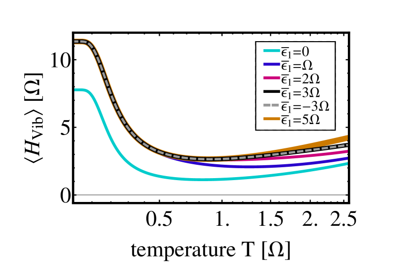
Figure S1: Average vibrational energy $\langle H_{\text{Vib}}\rangle$ for our minimal model of a molecular junction as a function of temperature for different level positions $\overline{\epsilon}_{1}$. These results have been obtained using BM and $\Phi=2(\overline{\epsilon}_{1}+3\Omega/2)$.

II Influence of other electronic states

Another important influence is exerted by the presence of other electronic levels. A higher-lying electronic level, for example, can facilitate additional inelastic processes that lead to a reduction of the vibrational energy at high bias voltages Härtle et al. (2009); Romano et al. (2010). A similar behavior can be observed in the presence of electron-electron interactions (Coulomb cooling) Härtle and Thoss (2011a). To study these effects, we add another electronic level to our model. It is distinguished from the first one only by its energy $\overline{\epsilon}_{2}=\epsilon_{2}-\lambda_{2}^{2}/\Omega$.

Fig. S2 shows the temperature dependence of the average vibrational energy $\langle H_{\text{Vib}}\rangle$ for different positions of the second electronic level, without electron-electron interactions $\overline{U}_{12}=U_{12}-2\lambda_{1}\lambda_{2}/\Omega=0$ (left panel of Fig. S2) and with electron-electron interactions $\overline{U}_{12}=5\Omega$ (right panel of Fig. S2). If the second state is too high in energy (red and blue lines), it has no effect. Once it approaches the bias window from above, resonant deexcitation processes with respect to this level become active and suppress the overall level of vibrational energy Härtle et al. (2009); Romano et al. (2010) and, consequently, the thermal stabilization effect (cf. turquoise line). Once it approaches the first level or becomes located below, the energy levels rise again and thermal stabilization is reestablished. These findings are very similar for both scenarios, with or without electron-electron interactions.

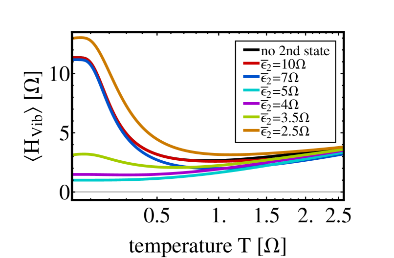
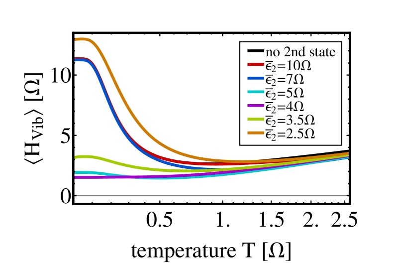
Figure S2: Average vibrational energy $\langle H_{\text{Vib}}\rangle$ for our minimal model of a molecular junction as a function of temperature, including a second electronic state that is located at a set of different energies $\overline{\epsilon}_{2}$. The left/right panel shows results for $\overline{U}_{12}=0$/$\overline{U}_{12}=5\Omega$. These results have been obtained using BM and $\Phi=2(\overline{\epsilon}_{1}+3\Omega/2)=9\Omega$.

References

- Piva et al. (2005) P. G. Piva, G. A. DiLabio, J. L. Pitters, J. Zikovsky, M. Rezeq, S. Dogel, W. A. Hofer, and R. A. Wolkow, Nature 435, 658 (2005).
- Song et al. (2009) H. Song, Y. Kim, Y. H. Jang, H. Jeong, M. A. Reed, and T. Lee, Nature 462, 1039 (2009).
- Loss and DiVincenzo (1998) D. Loss and D. P. DiVincenzo, Phys. Rev. A 57, 120 (1998).
- Petersson et al. (2011) K. D. Petersson, L. W. McFaul, M. D. Schroer, M. Jung, J. M. Taylor, A. A. Houck, and J. R. Petta, Nature 490, 380 (2011).
- Reed et al. (1997) M. A. Reed, C. Zhou, C. J. Muller, T. P. Burgin, and J. M. Tour, Science 278, 252 (1997).
- Reichert et al. (2002) J. Reichert, R. Ochs, D. Beckmann, H. B. Weber, M. Mayor, and H. v. Lohneysen, Phys. Rev. Lett. 88, 176804 (2002).
- Park et al. (2002) J. Park, A. N. Pasupathy, J. I. Goldsmith, C. Chang, Y. Yaish, J. R. Petta, M. Rinkoski, J. P. Sethna, H. D. Abruna, P. L. McEuen, et al., Nature (London) 417, 722 (2002).
- Reed (2004) M. A. Reed, Nature Materials 3, 286 (2004).
- Wu et al. (2004) S. W. Wu, G. V. Nazin, X. Chen, X. H. Qiu, and W. Ho, Phys. Rev. Lett. 93, 236802 (2004).
- Cuniberti et al. (2005) G. Cuniberti, G. Fagas, and K. Richter, Introducing Molecular Electronics (Springer, Heidelberg, 2005).
- Venkataraman et al. (2006) L. Venkataraman, J. E. Klare, C. Nuckolls, M. S. Hybertsen, and M. L. Steigerwald, Nature 442, 904 (2006).
- Secker et al. (2011) D. Secker, S. Wagner, S. Ballmann, R. Härtle, M. Thoss, and H. B. Weber, Phys. Rev. Lett. 106, 136807 (2011).
- Cuevas and Scheer (2010) J. C. Cuevas and E. Scheer, Molecular Electronics: An Introduction To Theory And Experiment (World Scientific, Singapore, 2010).
- Agrait et al. (2002) N. Agrait, C. Untiedt, G. Rubio-Bollinger, and S. Vieira, Chem. Phys. 281, 231 (2002).
- Agrait et al. (2003) N. Agrait, A. L. Yeyati, and J. M. van Ruitenbeek, Phys. Rep. 377, 81 (2003).
- Schäfer et al. (2009) J. Schäfer, S. Meyer, C. Blumenstein, K. Roensch, R. Claessen, S. Mietke, M. Klinke, T. Podlich, R. Matzdorf, A. A. Stekolnikov, et al., New J. Phys. 11, 125011 (2009).
- Blumenstein et al. (2011) C. Blumenstein, J. Schäfer, S. Mietke, S. Meyer, A. Dollinger, M. Lochner, X. Y. Cui, L. Patthey, R. Matzdorf, and R. Claessen, Nature Physics 7, 776 (2011).
- LeRoy et al. (2004) B. J. LeRoy, S. G. Lemay, J. Kong, and C. Dekker, Nature 432, 371 (2004).
- Tans et al. (1997) S. J. Tans, M. H. Devoret, H. Dai, A. Thess, R. Smalley, L. J. Geerligs, and C. Dekker, Nature 386, 6624 (1997).
- Sapmaz et al. (2005) S. Sapmaz, P. Jarillo-Herrero, Y. M. Blanter, and H. S. J. van der Zant, New J. Phys. 7, 243 (2005).
- Sapmaz et al. (2006) S. Sapmaz, P. Jarillo-Herrero, Y. M. Blanter, C. Dekker, and H. S. J. van der Zant, Phys. Rev. Lett. 96, 026801 (2006).
- Leturcq et al. (2009) R. Leturcq, C. Stampfer, K. Inderbitzin, L. Durrer, C. Hierold, E. Mariani, M. G. Schultz, F. von Oppen, and K. Ensslin, Nature Physics 5, 327 (2009).
- Delbecq et al. (2011) M. R. Delbecq, V. Schmitt, F. D. Parmentier, N. Roch, J. J. Viennot, G. Fève, B. Huard, C. Mora, A. Cottet, and T. Kontos, Phys. Rev. Lett. 107, 256804 (2011).
- Delbecq et al. (2013) M. R. Delbecq, L. E. Bruhat, J. J. Viennot, S. Datta, A. Cottet, and T. Kontos, Nat. Commun. 4, 1400 (2013).
- Reed et al. (1988) M. A. Reed, J. N. Randall, R. J. Aggarwal, R. J. Matyi, T. M. Moore, and A. E. Wetsel, Phys. Rev. Lett. 60, 535 (1988).
- van Wees et al. (1988) B. J. van Wees, H. van Houten, C. W. J. Beenakker, J. G. Williamson, L. P. Kouwenhoven, D. van der Marel, and C. T. Foxon, Phys. Rev. Lett. 60, 848 (1988).
- Holleitner et al. (2001) A. W. Holleitner, C. R. Decker, H. Qin, K. Eberl, and R. H. Blick, Phys. Rev. Lett. 87, 256802 (2001).
- van der Wiel et al. (2002) W. G. van der Wiel, S. De Franceschi, J. M. Elzerman, T. Fujisawa, S. Tarucha, and L. P. Kouwenhoven, Rev. Mod. Phys. 75, 1 (2002).
- Ihn et al. (2007) T. Ihn, M. Sigrist, K. Ensslin, W. Wegscheider, and M. Reinwald, New J. Phys. 9, 111 (2007).
- Kießlich et al. (2007) G. Kießlich, E. Schöll, T. Brandes, F. Hohls, and R. J. Haug, Phys. Rev. Lett. 99, 206602 (2007).
- Tutuc et al. (2011) D. Tutuc, B. Popescu, D. Schuh, W. Wegscheider, and R. J. Haug, Phys. Rev. B 83, 241308 (2011).
- Liu et al. (2014) Y. Y. Liu, K. D. Petersson, J. Stehlik, J. M. Taylor, and J. R. Petta, Phys. Rev. Lett. 113, 036801 (2014).
- Beckel et al. (2014) A. Beckel, A. Kurzmann, M. Geller, A. Ludwig, A. D. Wieck, J. König, and A. Lorke, Eur. Phys. Lett. 106, 47002 (2014).
- Lüffe et al. (2008) M. C. Lüffe, J. Koch, and F. von Oppen, Phys. Rev. B 77, 125306 (2008).
- Hüttel et al. (2009) A. K. Hüttel, B. Witkamp, M. Leijnse, M. R. Wegewijs, and H. S. J. van der Zant, Phys. Rev. Lett. 102, 225501 (2009).
- Härtle et al. (2009) R. Härtle, C. Benesch, and M. Thoss, Phys. Rev. Lett. 102, 146801 (2009).
- Romano et al. (2010) G. Romano, A. Gagliardi, A. Pecchia, and A. Di Carlo, Phys. Rev. B 81, 115438 (2010).
- McEniry et al. (2009) E. J. McEniry, T. N. Todorov, and D. Dundas, J. Phys.: Condens. Matter 21, 195304 (2009).
- Galperin et al. (2009) M. Galperin, K. Saito, A. V. Balatsky, and A. Nitzan, Phys. Rev. B 80, 115427 (2009).
- Gelbwaser-Klimovsky et al. (2017) D. Gelbwaser-Klimovsky, A. Aspuru-Guzik, M. Thoss, and U. Peskin, arXiv: 1705.08534 (2017).
- Lü et al. (2011) J. T. Lü, P. Hedegård, and M. Brandbyge, Phys. Rev. Lett. 107, 046801 (2011).
- Simine and Segal (2012) L. Simine and D. Segal, Phys. Chem. Chem. Phys. 14, 13820 (2012).
- Härtle and Thoss (2011a) R. Härtle and M. Thoss, Phys. Rev. B 83, 115414 (2011a).
- Brüggemann et al. (2014) J. Brüggemann, S. Weiss, P. Nalbach, and M. Thorwart, Phys. Rev. Lett. 113, 076602 (2014).
- Gordon and Ng (2000) M. Gordon and K. C. Ng, Cool Thermodynamics (Cambridge International Science Publishing, Cambridge, England, 2000).
- Palao et al. (2001) J. P. Palao, R. Kosloff, and J. M. Gordon, Phys. Rev. E 64, 056130 (2001).
- Linden et al. (2010) N. Linden, S. Popescu, and P. Skrzypczyk, Phys. Rev. Lett. 105, 130401 (2010).
- Levy and Kosloff (2012) A. Levy and R. Kosloff, Phys. Rev. Lett. 108, 070604 (2012).
- Cleuren et al. (2012) B. Cleuren, B. Rutten, and C. Van den Broeck, Phys. Rev. Lett. 108, 120603 (2012).
- Gelbwaser-Klimovsky and Kurizki (2014) D. Gelbwaser-Klimovsky and G. Kurizki, Phys. Rev. E 90, 022102 (2014).
- Gelbwaser-Klimovsky et al. (2015) D. Gelbwaser-Klimovsky, W. Niedenzu, and G. Kurizki, Adv. At. Mol. Opt. Phys. 64, 329 (2015).
- Mari and Eisert (2012) A. Mari and J. Eisert, Phys. Rev. Lett. 108, 120602 (2012).
- Mitra et al. (2004) A. Mitra, I. Aleiner, and A. J. Millis, Phys. Rev. B 69, 245302 (2004).
- Koch et al. (2006) J. Koch, M. Semmelhack, F. von Oppen, and A. Nitzan, Phys. Rev. B 73, 155306 (2006).
- Avriller (2011) R. Avriller, J. Phys.: Condens. Matter 23, 105301 (2011).
- Härtle and Thoss (2011b) R. Härtle and M. Thoss, Phys. Rev. B 83, 125419 (2011b).
- Kast et al. (2011) D. Kast, L. Kecke, and J. Ankerhold, Beilstein J. Nanotechnol. 2, 416 (2011).
- Härtle and Kulkarni (2015) R. Härtle and M. Kulkarni, Phys. Rev. B 91, 245429 (2015).
- Mukamel and Smalley (1980) S. Mukamel and R. E. Smalley, J. Chem. Phys. 73, 4156 (1980).
- Freed and Nitzan (1983) K. F. Freed and A. Nitzan, Energy Storage and Redistribution in Molecules (Plenum, New York, 1983).
- Zewail (1994) A. H. Zewail, Femtochemistry – Ultrafast Dynamics of the Chemical Bond (World Scientific, Singapore, 1994).
- Nesbitt and Field (1996) D. J. Nesbitt and R. W. Field, J. Phys. Chem. 100, 12735 (1996).
- Tao (2006) N. J. Tao, Nat. Nano. 1, 173 (2006).
- Jorn and Seidemann (2009) R. Jorn and T. Seidemann, J. Chem. Phys. 131, 244114 (2009).
- May (2002) V. May, Phys. Rev. B 66, 245411 (2002).
- Lehmann et al. (2004) J. Lehmann, S. Kohler, V. May, and P. Hänggi, J. Chem. Phys. 121, 2278 (2004).
- Harbola et al. (2006) U. Harbola, M. Esposito, and S. Mukamel, Phys. Rev. B 74, 235309 (2006).
- Volkovich et al. (2008) R. Volkovich, M. Caspary Toroker, and U. Peskin, J. Chem. Phys. 129, 034501 (2008).
- Pshenichnyuk and Čížek (2011) I. A. Pshenichnyuk and M. Čížek, Phys. Rev. B 83, 165446 (2011).
- Schinabeck et al. (2016) C. Schinabeck, A. Erpenbeck, R. Härtle, and M. Thoss, Phys. Rev. B 94, 201407 (2016).
- Jin et al. (2008) J. Jin, X. Zheng, and Y. Yan, J. Chem. Phys. 128, 234703 (2008).
- König and Martinek (2003) J. König and J. Martinek, Phys. Rev. Lett. 90, 166602 (2003).
- Wunsch et al. (2005) B. Wunsch, M. Braun, J. König, and D. Pfannkuche, Phys. Rev. B 72, 205319 (2005).
- Härtle and Millis (2014) R. Härtle and A. J. Millis, Phys. Rev. B 90, 245426 (2014).
- Härtle et al. (2013) R. Härtle, G. Cohen, D. R. Reichman, and A. J. Millis, Phys. Rev. B 88, 235426 (2013).
- Hell et al. (2015) M. Hell, B. Sothmann, M. Leijnse, M. R. Wegewijs, and J. König, Phys. Rev. B 91, 195404 (2015).
- Wenderoth et al. (2016) S. Wenderoth, J. Bätge, and R. Härtle, Phys. Rev. B 94, 121303R (2016).
- Härtle et al. (2010) R. Härtle, R. Volkovich, M. Thoss, and U. Peskin, J. Chem. Phys. 133, 081102 (2010).
- Volkovich et al. (2011) R. Volkovich, R. Härtle, M. Thoss, and U. Peskin, Phys. Chem. Chem. Phys. 13, 14333 (2011).