The SPHINX Cosmological
Simulations of the First Billion Years:
the Impact of Binary Stars
on Reionization††thanks: https://sphinx.univ-lyon1.fr/
Abstract
We present the Sphinx suite of cosmological adaptive mesh refinement simulations, the first radiation-hydrodynamical simulations to simultaneously capture large-scale reionization and the escape of ionizing radiation from thousands of resolved galaxies. Our and co-moving Mpc volumes resolve haloes down to the atomic cooling limit and model the inter-stellar medium with better than pc resolution. The project has numerous goals in improving our understanding of reionization and making predictions for future observations. In this first paper we study how the inclusion of binary stars in computing stellar luminosities impacts reionization, compared to a model that includes only single stars. Owing to the suppression of galaxy growth via strong feedback, our galaxies are in good agreement with observational estimates of the galaxy luminosity function. We find that binaries have a significant impact on the timing of reionization: with binaries, our boxes are percent ionized by volume at , while without them our volumes fail to reionize by . These results are robust to changes in volume size, resolution, and feedback efficiency. The escape of ionizing radiation from individual galaxies varies strongly and frequently. On average, binaries lead to escape fractions of percent, about times higher than with single stars only. The higher escape fraction is a result of a shallower decline in ionizing luminosity with age, and is the primary reason for earlier reionization, although the higher integrated luminosity with binaries also plays a sub-dominant role.
keywords:
early Universe – dark ages, reionization, first stars – galaxies: high-redshift – methods: numerical1 Introduction
The formation of the first galaxies marks the end of the dark ages and the beginning of the Epoch of Reionization (EoR). Radiation from the first generations of stars, hosted by the first galaxies, heated the surrounding inter-galactic gas via photo-ionization. As the ionized hydrogen () bubbles grew and percolated, the whole Universe was transformed from a dark, cold, neutral state into a hot ionized one: reionization was completed. This last major transition of the Universe is at the limit of our observational capabilities and is a key science driver of the foremost upcoming telescopes, such as the James Webb Space Telescope (JWST) and the Square Kilometre Array (SKA).
Cosmological simulations are an indispensable tool to disentangle the complex and non-linear interplay of physical mechanisms leading to reionization, a ‘loop’ encompassing an enormous range of physical scales: of gravitational collapse of dark matter into haloes, the condensation of gas via radiative cooling into galaxies at the centers of those haloes, it’s eventual collapse into stars, which is slowed down by feedback, the emission of ionizing radiation from those stars, the propagation of the radiation through the inter-stellar medium (ISM), the circum-galactic medium (CGM) and the inter-galactic medium (IGM), and its ability to suppress gas cooling and thus star formation.
Two major challenges face those seeking to understand reionization with simulations, compared with simulations of galaxy evolution at low-redshift. First is the need for radiation-hydrodynamics (RHD) to explicitly model the interplay of ionizing radiation and gas. Traditional cosmological simulations use pure gravito-hydrodynamics, typically applying homogeneous ultra-violet (UV) background radiation instead of the more computationally expensive hydrodynamically coupled radiative transfer. However, to model the reionization process self-consistently, the radiation should not be ignored or applied in post-processing. The second challenge is capturing the range of scales involved. Reionization is a large-scale process that should preferentially be modelled on cosmological-homogeneity scales, or volume widths of co-moving Mpc (cMpc), in order to predict the patchiness of reionization and a realistic average volume filling factor of ionized gas that is unaffected by cosmic variance (Iliev et al., 2013). The sources of reionization, however, form and emit radiation on relatively tiny, sub-pc scales, and even if sub-pc scales are not represented, predicting the transfer and escape of ionizing radiation through the ISM requires at least a few pc resolution (e.g. Kimm & Cen, 2014; Xu et al., 2016).
There has been a surge of cosmological RHD reionization simulation projects that have captured the large-scale reionization process (Gnedin & Fan, 2006; Finlator et al., 2011; Iliev et al., 2013; Gnedin, 2014; So et al., 2013; Pawlik et al., 2016; Ocvirk et al., 2015; Chen et al., 2017), with volume widths ranging from cMpc. However, the range of scales required to adequately model both the large-scale process and the production and transfer of radiation through the ISM has been out of reach. Galaxies are still largely unresolved in reionization simulations, with physical resolution ranging from pc (Gnedin, 2014; Pawlik et al., 2016) for smaller volumes to kpc (Iliev et al., 2013) for the largest ones. Therefore, the escape fraction of ionizing radiation from galaxies, , is fully or partly a free and adjustable parameter. If galaxies are not resolved at all it sets the total fraction of radiation getting out of galaxies. If galaxies are to some degree resolved, the free parameter is a sub-resolution escape fraction, , setting the luminosity of stellar sources, and the real escape fraction becomes a multiple of , which sets the production rate of ionizing photons, and the fraction of emitted radiation that propagates out of galaxies (e.g. Pawlik et al., 2016).
Cosmological zoom simulations can achieve a much higher maximum resolution than full cosmological simulations by focusing only on the environment of one or a few haloes with a nested refinement structure. In this type of simulation, the production and escape of ionizing radiation in galaxies can be predicted in detail, even with sub-parsec resolution. Furthermore, fewer assumptions regarding star formation, feedback, and radiation-gas interactions are required. Radiation-hydrodynamical zoom simulations have provided important insight into reionization and particularly how appears to highly fluctuate and be strongly regulated by feedback (Wise & Cen, 2009; Kimm & Cen, 2014; Wise et al., 2014; Trebitsch et al., 2017a; Xu et al., 2016; Kimm et al., 2017). However, the sacrifice is that the large-scale reionization process, statistical averages, and the scatter (in e.g. and ionizing luminosities against galaxy properties) provided by the resolved evolution of many haloes is lost. The cosmological environment surrounding these few targeted well-resolved haloes remains at a relatively low resolution and only serves to provide a realistic background gravitational field.
The recent state-of-the-art is to connect these two types of small-scale and large-scale simulations by using the predicted escape of photons from the high-resolution zooms as inputs for the unresolved escape of photons from galaxies in full reionization simulations, allowing predictions to be made for the contributions of different galaxy masses to reionization (Xu et al., 2016; Chen et al., 2017). Yet, this approach still lacks the full coupling between the highly fluctuating escape of ionizing radiation from these unresolved galaxies and the galaxy dynamics, which is partially regulated by large-scale processes of mergers and accretion. Full non-zoom cosmological RHD simulations of reionization that capture these large scale processes and simultaneously predict the production and escape of ionizing radiation remain the ideal goal.
With recent increase in computational power and algorithmic advances for radiation-hydrodynamics in the Ramses-RT code, this goal is now within reach. Here, we present the Sphinx111In the spirit of the mythical Sphinx, we prefer to keep the acronym an enigma. suite of simulations, a series of cosmological volumes cMpc in width where haloes are well resolved down to or below the atomic cooling threshold (halo mass of ; Wise et al. 2014) and a maximum physical resolution of pc is reached in the ISM of galaxies at (and higher at higher redshifts).
These volumes are still well below the cosmological homogeneity scale, but we apply an initial conditions (ICs) selection technique that allows us to minimise cosmic variance effects, model an accurate ionizing photon production rate, and achieve reionization histories that are well-converged with simulation volume. The simulation volumes include thousands of star-forming galaxies, allowing for a statistical understanding of escape fractions and ionizing luminosities for haloes over a mass range of .
Our goals with the Sphinx project are numerous, including understanding the main sources of reionization (e.g. halo masses, environments, stellar population ages), the statistical behaviour of , and the back-reaction (Gnedin & Kaurov, 2014) of radiation on the formation of dwarf galaxies. Furthermore, we aim to make predictions for the observational signatures of EoR galaxies for the JWST and to better constrain the metal enrichment process of the high-redshift IGM. These goals will be addressed in forthcoming papers. This pilot Sphinx paper is dedicated to describing the numerical methods and setup of our simulations, to comparing our simulated galaxies to observations of the high-redshift Universe, and to addressing the contribution of binary stars to reionization.
Recently, Stanway et al. (2016) demonstrated how accounting for the interactions of binary stars in spectral energy distribution (SED) models increases the total flux of ionizing radiation from metal-poor stellar populations by tens of percent, compared to models that do not include binaries. Around the same time, Ma et al. (2016) demonstrated an additional, and perhaps more important, effect of binaries, which is an increase in the escape of ionizing radiation from galaxies. They post-processed cosmological zoom simulations with ray-tracing, comparing two sets of SED models, with only single stars, and with added binary stars, and found a factor higher with binary stars included (with for binaries).
This ties to the regulation of by stellar feedback. In the first few Myr after the birth of a stellar population, very little ionizing radiation escapes, even if the population is very luminous, since the radiation is absorbed locally by the dense ISM. The first SN explosions at Myr coincide with a steep drop in the production rate of ionizing photons, because the most luminous stars in the population are precisely those most massive ones that explode first as SNe. So as the ISM starts to be cleared away by SN explosions and the radiation begins to escape, the ionizing luminosity is rapidly declining, resulting in an overall small fraction of the emitted radiation escaping. Due to mass transfer and mergers between binary companions, UV luminous stars exist at much later times in models that include binaries compared to single stars only models. The luminosity still declines after Myr, but at a slower rate, enhancing the number of photons that can escape into the IGM after the onset of SN explosions.
Ma et al. (2016) predict a strong boost in with the inclusion of binary stars, but they apply the radiative transfer in post-processing and only consider three galaxies from cosmological zoom simulations. Therefore they do not consider the back reaction on the gas or predict how binary stars affect the reionization history. In this paper, we seek to verify and expand the results of Ma et al. (2016), using directly coupled radiation-hydrodynamics, and a full (non-zoom) cosmological volume to provide the statistics of thousands of galaxies. This allows us to directly probe whether and how the inclusion of binary stars affects the evolution, observational properties, and escape fractions of galaxies, as well as the timing and the process of reionization.
The setup of the paper is as follows. In section 2 we present our simulation methods and setup (code, refinement, radiative transfer, star formation, feedback, selection of initial conditions). In section 3 we present our results, first comparing our simulations with observables, then showing the reionization histories resulting from binary and single star SED models, and finally comparing overall escape fractions, with those same models, from millions of stellar populations in thousands of galaxies. We present our discussion of the greater impact of binaries on reionization in section 4 and conclude in section 5 by highlighting upcoming work using the Sphinx simulations.
2 Simulations
We use Ramses-RT (Rosdahl et al., 2013; Rosdahl & Teyssier, 2015), which is an RHD extension of the cosmological gravito-hydrodynamical code Ramses (Teyssier, 2002)222The public code, including all the RHD extensions used here, can be downloaded at https://bitbucket.org/rteyssie/ramses, to solve the interactions of dark matter, stellar populations, ionizing radiation, and baryonic gas via gravity, hydrodynamics, radiative transfer, and non-equilibrium radiative cooling/heating, on a three-dimensional adaptive mesh. For the hydrodynamics, we use the HLLC Riemann solver (Toro et al., 1994) and the MinMod slope limiter to construct gas variables at cell interfaces from their cell-centred values. To close the relation between gas pressure and internal energy, we use an adiabatic index , which is appropriate for an ideal monatomic gas. The dynamics of collisionless DM and stellar particles are evolved with a particle-mesh solver and cloud-in-cell interpolation (Guillet & Teyssier, 2011). The advection of radiation between cells is solved with a first-order moment method, using the fully local M1 closure for the Eddington tensor (Levermore, 1984) and the Global-Lax-Friedrich flux function for constructing the inter-cell radiation field.
In the following sub-sections, we describe the set-up of our simulations (initial conditions, adaptive refinement, ionizing radiation, thermochemistry), our main sub-grid model components (star formation and supernova feedback), and the halo finder utilised in the analysis. For reference, the main simulation parameters are listed in Table 1.
| Name | Value | Comments |
|---|---|---|
| Initial conditions (ICs) mass density | ||
| ICs dark energy density | ||
| ICs baryon density | ||
| ICs amplitude of galaxy fluctuations | ||
| Hubble constant | ||
| Hydrogen mass fraction | ||
| Helium mass fraction | ||
| Initial metal mass fraction | ||
| SN ejecta mass fraction | ||
| Mean SN progenitor mass | ||
| SN metal yield |
2.1 Halo finder
For identification of haloes and galaxies, we use the AdaptaHOP halo finder (Aubert et al., 2004; Tweed et al., 2009) in the most massive submaxima (MSM) mode. We fit a tri-axial ellipsoid to each (sub-)halo and check that the virial theorem is satisfied within this ellipsoid, with the center corresponding to the location of the densest particle. If this condition is not satisfied, we iteratively decrease its volume until we reach an inner virialized region. From the volume of this largest ellipsoidal virialized region, we define the virial radius and mass . We have checked that our results are similar if we instead use and , defined to produce a spherical over-density times the critical value. For the halo finder, we require a minimum of particles per halo. In practice, using the notation of Aubert et al. (2004, App. B) we use for the halo finder , , , and . We also require that a (sub-)group of particles has at least particles during the halo/sub-halo decomposition step. In the end, we retain for the analysis only those haloes we consider resolved, with , where is the DM particle mass. For this work, we also ignore sub-haloes in our analysis.
We also identify galaxies with AdaptaHOP. Here we require at least stellar particles per galaxy and we add sub-groups to the main bodies. The galaxy-finder parameters are: , , , and .
2.2 Initial conditions
We generate the cosmological initial conditions (ICs) with Music (Hahn & Abel, 2011). Our CDM universe has cosmological parameters , , , , and , consistent with the Planck 2013 results (Planck Collaboration, 2014). We assume hydrogen and helium mass fractions and , respectively, and the gas is given an initial homogeneous metal mass fraction of (we assume a Solar metal mass fraction of throughout this work). This unrealistically non-pristine initial metallicity is used to compensate for our lack of molecular hydrogen cooling channels in the infant Universe, allowing the gas to cool below K, and calibrated so that the first stars form at redshift .
| Name | |||||
|---|---|---|---|---|---|
| [cMpc] | [] | [] | |||
| S10_512 | kpc | pc | |||
| S05_512 | kpc | pc | |||
| S05_256 | kpc | pc |
We use three sets of initial conditions with two volume sizes, as listed in Table 2. Our main simulation volume, S10_512, has a width of cMpc, a minimum (coarse) physical resolution of ckpc ( kpc at ), and reaches a maximum cell resolution of cpc ( pc at ). It is populated by DM particles with mass each. We assume the limit of a resolved halo being at a mass corresponding to DM particles. This means we resolve haloes down to a mass of , which is slightly above the atomic cooling limit of (Wise et al., 2014). The atomic cooling limit is important because below it, primordial galaxies form inefficiently and likely contribute little to reionization due to their self-destructive behaviour (Kimm et al., 2017). To measure the possible contribution from low-mass haloes that are above the atomic cooling limit but unresolved in the S10_512 volume (i.e. at masses ), we use volume S05_512, with the same number of DM particles but half the width, thus giving an eight times higher DM mass resolution, or , and haloes resolved down to . Statistical representation of massive haloes is sacrificed, due to the smaller volume, to the gain of resolving haloes down to the atomic cooling limit. This allows us to probe the contribution of the smallest haloes to reionization. We keep the maximum physical resolution in this volume the same as in S10_512, i.e. pc at , but the coarse resolution is higher, following the DM resolution, or kpc at .
The third simulation volume, S05_256, connects the other two volumes by having the resolution of the larger volume, S10_512, and size and initial conditions of the the smaller volume, S05_512. Hence we can use it for resolution convergence studies, by comparing the properties of galaxies to those in S05_512.
2.2.1 Volume selection
Our simulation volumes do not probe the scales at which the Universe is homogeneous. Hence we are influenced by cosmic variance, such that different IC realisations, with different random seeds for the generation of density fluctuations, result in different halo mass functions at later epochs. This can, in turn, affect the luminosity function and change the reionization history.

To recover a representative luminosity density and reionization history from our limited-volume simulations, we seek to minimise the effects of cosmic variance on the ionizing luminosity budget by selecting the most representative ICs from a large set of candidates. We perform pure DM simulations at a degraded resolution of for both the and cMpc wide volumes, each starting from ICs generated with a unique set of random number seeds. We then select from those the ICs that give the most average cumulative DM halo mass function to the power of , , at , and . We use rather than because we find that it correlates better with the total luminosity of galaxies: the ionizing luminosity scales linearly with the star formation rate, which scales roughly as (see Fig. 6).
Fig. 1 shows the cumulative functions at and for the pure DM runs of the cMpc ICs in coloured curves, and the averages of all simulations in thick dashed black curves. Our selected ICs are represented by thick coloured curves, at the degraded DM mass resolution in solid and the fiducial resolution in dashed. A comparison of the thick coloured solid and dashed curves shows that the DM resolution has little effect on the cumulative halo mass function (but note that it does have an impact on the non-cumulative function at the low-mass end, since low-mass haloes are lost when degrading the resolution). Out of candidate ICs, it is difficult to get an ideal average at all three redshifts. The selected ICs are very close to the average at and , but slightly top-heavy at and thus perhaps produce slightly too many stars at .
Fig. 2 shows the number of haloes in our two simulation volumes, binned by halo mass. At , each volume contains about haloes above the resolution limit. The smaller and larger volumes have maximum halo masses of and , respectively, at .

2.3 Adaptive refinement
In the cubical octree structure of Ramses, the cell refinement level sets the cell width , where is the width of the volume. Taking our cMpc volume, the coarsest level is , corresponding to coarse cell widths and a minimum resolution of ckpc ( kpc at ). Starting at this coarsest level, cells are adaptively refined to higher levels, up to , which corresponds to a maximum physical resolution of pc at .
| Photon | [eV] | [eV] | [Å] | [Å] | [eV] | |||
| group | ||||||||
| UV | 13.6 | 24.59 | 18.3 | 0 | 0 | |||
| UV | 24.59 | 54.42 | 33.9 | 0 | ||||
| UV | 54.42 | 0 | 63.3 |
A cell is flagged for refinement into equally sized children cells if: i) , where and are the total DM and baryonic (gas plus stars) masses in the cell, or ii) the cell width is larger than a quarter of the local Jeans length,
| (1) |
where is the speed of sound, the gravitational constant, the gas mass density, and the hydrogen number density.
Contrary to the default refinement strategy in Ramses, which is to increase the maximum refinement level at fixed scale factor intervals to roughly maintain a constant maximum physical resolution, we keep the maximum refinement level fixed throughout the simulation. Hence the minimum physical cell widths are smaller at the start of the simulation than at . The difference in minimum cell size is not much different than at though, since the maximum level is first triggered at and thus the finest cells are times smaller (i.e. pc) than at .
The resolution of the gravitational force is the same as that of the gas, with the gravitational potential calculated for each cell. In the fiducial-resolution S05_256 and S10_512 runs, the DM density is smoothed to the second-finest levels, whereas in the high-resolution S05_512 runs, the DM density is applied to the finest level. This smoothing of the DM density is decided from analogue pure DM simulations using the refinement criteria stated above but without any limit in the maximum refinement. The maximum refinement actually reached in those pure DM simulations sets the maximum DM density level: for the high-resolution RHD simulations but for the fiducial resolution.
2.4 Radiation
The methods for photon injection, M1 moment advection, and the interaction of radiation with hydrogen and helium gas via photo-ionization, heating, and direct radiation pressure, are fully described in Rosdahl et al. (2013). The radiation is split into three photon groups, bracketed by the ionization energies for , , and , and shown in Table 3. Radiation interacts with hydrogen and helium via photo-ionization, heating, and momentum transfer (Rosdahl & Teyssier, 2015). The group properties (average energies and cross sections to hydrogen and helium) are updated every coarse time-steps from luminosity-weighted averages of the spectra of all stellar populations in the simulation volume, as described in Rosdahl et al. (2013). We do this so that at any time, the cross sections and photon energies are representative of the average photon population. Hence, as indicated in the Table 3 (and Fig. 23 in Appendix D), the energies and cross sections change by a few tens of percent over the course of a simulation as the contributions from both old and metal-rich stellar populations increases.
In this work, we ignore the effects of radiation at sub-ionizing energies ( eV). We have run a sub-set of small-volume simulations at the fiducial resolution with added optical and reprocessed infrared radiation groups, and including multi-scattering radiation pressure on dust as described in Rosdahl & Teyssier (2015); Rosdahl et al. (2015), but found a negligible impact. This is likely because of the low metal and dust content at the early epoch we are concerned with.
Radiation is advected on the grid with an explicit solver, and therefore the simulation time-step is subject to the Courant condition. Since the radiative transfer (RT) time-step can become significantly smaller than the hydrodynamic time-step, we subcycle the RT on each AMR level, with a maximum of RT steps performed after each hydro step (if the projected number of RT steps exceeds , the hydro time-step length is decreased accordingly). During the sub-cycling on each level, radiation is prevented from propagating to other levels and the radiation flux across boundaries is treated with Dirichlet boundary conditions: when advecting radiation on grid refinement level , the radiation density and flux in neighbouring cells at the finer () and coarser () levels is fixed at the states from the last RT steps performed at those levels. Radiation can cross boundaries into the level currently being sub-cycled, but to prevent ‘bursts’ of radiation across level boundaries, levels are not updated when sub-cycling level : these updates are performed only when those other levels are being RT sub-cycled. In this scheme, perfect photon conservation is not strictly maintained across level boundaries, although we have verified with tests that the number of photons is conserved to the level of a few percent or less. For details of the same sub-cycling scheme in the context of flux-limited diffusion, see Commerçon et al. (2014).
To prevent prohibitively small time-steps and a large number of RT subcycles, we use the variable speed of light approximation (VSLA) described in Katz et al. (2017), with a local speed of light reduced by a factor from the real speed of light . Here, we apply a relatively slow speed of light in the finest grid cells, which typically represent the ISM of galaxies, and increase the speed of light by a factor two for every coarser level, up to a light speed fraction in the coarsest cells. These correspond to diffuse voids in the simulation volume (to be precise, the coarsest cells all have density less than eight times the critical density). This naturally follows the velocity increase of ionization fronts with lower gas density (Rosdahl et al., 2013) and allows us to reduce the cost of the calculation by reducing the speed of light in the regions that constrain the global time step.
In our cMpc volume, the speed of light fraction is set to for refinement levels , and is fixed at for . Even with the VSLA, using the full speed of light at the coarsest level(s) is prohibitively expensive. However, Katz et al. (2018) show that the reionization history is fairly well converged with this setup (see also Gnedin, 2016). The main deviations are overshoot in the volume-weighted neutral fraction, , during the final stage of reionization, when voids are being ionized, and a few tens of percent overshoot (undershoot) in the volume-weighted neutral fraction (photo-ionization rate) when the volume is completely reionized. For our comparison between SED models, these VLSA effects are negligible. Note that the variable speed of light conserves the total number of photons. The density of photons for group , varies locally and inversely with the speed of light, but the flux, remains exactly constant (see Rosdahl et al., 2013; Katz et al., 2017).
With our set-up for RT sub-cycling and the VSLA, the radiative transfer is rarely sub-cycled more than times on any given level. The only exception to this occurs early on in the simulations when the first stars have just been born and are emitting ionizing photons but SN have yet to occur. In this case, the hydro time steps are still very long compared to the RT time steps.
2.4.1 Single and binary star radiation sources
In this work, we compare the stellar emission from two SED models; the Galaxev model of Bruzual & Charlot (2003)333 www.bruzual.org/bc03/Updated_version_2016/BC03_basel_kroupa.tgz and the Binary Population and Spectral Synthesis code (Bpass: Eldridge et al., 2007; Stanway et al., 2016)444http://bpass.auckland.ac.nz/2.html. The latter includes binary stars while the former does not; for simplicity, we refer to the Bruzual & Charlot (2003) model as singles and the Bpass model as binaries throughout this paper.
For the single stars, we use the model generated with the semi-empirical BaSeL 3.1 stellar atmosphere library (Westera et al., 2002) and a Kroupa (2001) initial mass function (IMF). For the binaries we use the available IMF closest to Kroupa (2001), with slopes of from to and from to . In Appendix D we describe in detail how we extract luminosities and photon group properties from the assumed SEDs, and show how the group properties evolve with age and metallicity.

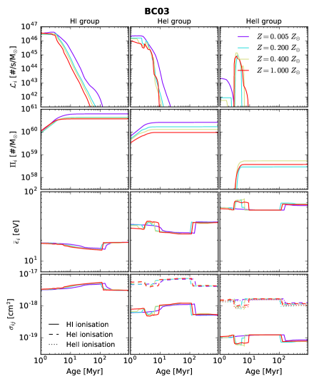
Fig. 3 shows the instantaneous and integrated luminosities ( and , respectively) for the two sets of SED models, for Solar metallicity () and , which is the lowest metallicity available in Bpass555For the Bruzual & Charlot (2003) model, we have used the interpolation scheme in Ramses-RT to retrieve the low metallicity curve and compare with Bpass, since the exact metallicity of th Solar is not tabulated in the official distribution. . There are two important differences to note. First, for low metallicity, the binaries model emits almost twice as many ionizing photons than the singles model. Second, at any metallicity, the ionizing luminosity decreases significantly faster with stellar age for the singles model compared to the binaries. For example, for , a singles population emits , , and of its ionizing photons in the first , , and Myr, respectively (the total is taken at Gyr, where the model ends), while the binaries population has emitted only , , and of all its ionizing photons at the same ages.
Both differences may cause the binaries SED model to reionize the Universe earlier than the singles model. However, simply increasing the number of available photons by a small factor does not necessarily cause significantly earlier reionization, as the radii of ionization bubbles scale only as luminosity to the power of one-third (Strömgren, 1939). The more prolonged emission with binaries is likely more important because what matters most is how many photons escape the dense ISM and penetrate out into the low density IGM where only photon per baryon is required to maintain ionization. Due to the interplay with stellar feedback, a stellar population is born in dense gas where the ionizing radiation is absorbed very efficiently in keeping up with the rapid rate of hydrogen recombinations, but as the population gets older, feedback processes can clear away the gas, allowing ionizing radiation to escape into the IGM (Kimm & Cen, 2014; Ma et al., 2016; Kimm et al., 2017; Trebitsch et al., 2017a).
2.4.2 Unresolved escape fractions
In previous simulations of reionization, the escape fraction of ionizing radiation on unresolved scales, , is typically calibrated such that the injected radiation is either higher or lower than that given by the SED model used. A sub-unity is then interpreted as modelling under-resolved over-densities, correcting for underestimated recombination rates and too many photons escaping the unresolved region, while models boost the luminosity of stellar sources to compensate for e.g. under-resolved escape channels, under-resolved turbulence (Safarzadeh & Scannapieco, 2016), or secondary ionization from X-ray binaries (Shull & van Steenberg, 1985). The calibration on is usually done in such a way that the Universe is reionized at the roughly the correct redshift (, depending on the definition of ‘reionized’), as determined from observations.
In this work we do not perform calibration on unresolved escape fractions, always setting . This does not mean that we are sure to fully resolve the escape of ionizing radiation from sources deep within galaxies. However, since we are primarily interested in comparing reionization histories and escape fractions with two different SED models, and since we find that the two SED models result in reionization histories that bracket current observational constraints, there is no particular need for calibration. This nonessential calibration of can be interpreted as either a balance between under-resolved clumps and under-resolved escape channels, or, more likely, an indication that the escape of radiation is governed more by large-scale feedback, captured with pc resolution, than the detailed turbulent motions of gas on pc and sub-pc scales.
2.5 Gas thermochemistry
The non-equilibrium hydrogen and helium thermochemistry, coupled with the local ionizing radiation, is performed with the quasi-implicit method described in Rosdahl et al. (2013) via photo-ionization, collisional ionization, collisional excitation, recombination, bremsstrahlung, homogeneous Compton cooling/heating off the cosmic-microwave background, and di-electronic recombination. Along with the temperature, and photon fluxes, we track in every cell the ionization fractions of hydrogen, singly, and doubly ionized helium (, , , respectively), and advect them with the gas, like the metal mass fraction, as passive scalars. The thermochemistry is operator split from the advection of gas and radiation and performed with adaptive-time-step sub-cycling on every RT time-step (i.e. the thermochemistry is sub-cycled within the RT, which is sub-cycled within the hydrodynamics). To reduce the amount of thermochemistry sub-cycling, we use the ‘smoothing’ method for un-splitting the advection and injection of photons from the thermochemistry, described in Rosdahl et al. (2013). We assume the on-the-spot approximation, whereby we ignore recombination emission of ionizing photons, assuming it is all absorbed locally, within the same cell.
For K, the cooling contribution from metals is computed using tables generated with Cloudy (Ferland et al., 1998, version 6.02), assuming photo-ionization equilibrium with a Haardt & Madau (1996) UV background. The metal cooling is not currently modelled self-consistently with the local radiation, which is a feature reserved for future work. For K, we use the fine structure cooling rates from Rosen & Bregman (1995), allowing the gas to cool radiatively to a density-independent temperature floor of K. We do not apply a density-dependent pressure floor to prevent numerical fragmentation: our star formation model (see below) is designed to very efficiently form stars at high gas densities and, in unison with SN and radiation feedback, prevent overly high densities and numerical fragmentation.
2.6 Star formation
We use the turbulent star formation (SF) criterion inspired by Federrath & Klessen (2012), as described in Kimm et al. (2017); Trebitsch et al. (2017a), and Devriendt (2018, in preparation).
The following conditions must be met locally for stars to form in a cell:
-
1.
The local hydrogen density and the local overdensity is more than a factor greater than the cosmological mean (the latter is needed to prevent ubiquitous star formation at extremely high redshift).
- 2.
-
3.
The gas is locally convergent and at a local density maximum compared to the six next-neighbour cells.
Gas that satisfies the above criteria is converted into stellar population particles at a rate
| (3) |
where is the local free-fall time and is the star formation efficiency. The cell gas is stochastically converted into collisionless stellar particles by sampling the Poisson probability distribution for gas to star conversion over the time-step (see Rasera & Teyssier, 2006, for details), such that on average, the conversion rate follows Eq. (3). The initial mass of each stellar particle is an integer multiple of , but capped so that no more than of the gas is removed from the cell. The main distinction of this turbulent star formation recipe from traditional star formation in Ramses (Rasera & Teyssier, 2006), where is a global (typically small) constant, is that varies locally with the thermo-turbulent properties of the gas (see Kimm et al., 2017; Trebitsch et al., 2017a; Devriendt, 2018, for details). The local star formation efficiency can approach and even exceed (with meaning that stars are formed faster than in a free-fall time). This gives rise to a bursty mode of star formation, whereas the classical constant recipe leads to star formation that is more smoothly distributed in both space and time.
We modify the SF recipe as described by Kimm et al. (2017) by subtracting rotational velocities and symmetric divergence from the turbulent velocity dispersion in Eq. (2) and the expression leading to , such that the turbulence represents only anisotropic and unordered motion. This leads to stronger instantaneous star formation at the centers of galaxies and rotating clouds, but also stronger feedback episodes, with the net effect of reducing the overall star formation.
2.7 Supernova feedback
We apply individual type II SN explosions of erg by stochastically sampling the delay-time distribution for the IMF over the first Myr of the lifetime of each stellar particle.
We use the mechanical SN model for momentum injection from Kimm et al. (2015, see also , and a similar model described in ). The key feature of the mechanical feedback model is its ability to capture the correct final snow-plow momentum of a SN remnant, by injecting it directly if the previous adiabatic phase is not resolved, or otherwise letting it evolve naturally. We review here the main features of the algorithm.
For one SN explosion, its radial momentum, along with the SN ejecta mass (), as well as gas mass contained in the host SN cell, is shared between the host and all neighbour cells sharing vertices with it (corners included; thermal energy is injected into the host instead of momentum). The amount of momentum given to each neighbour depends on the mass loading . Here, the denominator is the SN ejecta mass received by the neighbour, with a geometrical factor determining the share of SN energy and mass that the neighbour receives (totalling to unity for each explosion). The numerator, , contains all the mass in the same neighbour after the wind injection (i.e. the mass already in the cell plus the SN remnant plus times the mass originally in the SN host cell).
For low , the momentum injection follows the adiabatic phase with
| (4) |
Here, is a function ensuring a smooth transition to the maximum momentum injection for the neighbour,
| (5) |
where is the SN energy in units of ergs and always unity in these simulations, is the local hydrogen number density in units of , and . This expression for the density- and metallicity-dependent upper limit for the snowplow momentum comes from the numerical experiments of Blondin et al. (1998) and Thornton et al. (1998) of explosions in a homogeneous medium and has been confirmed more recently by e.g. Kim & Ostriker (2015) and Martizzi et al. (2015).
As in Kimm et al. (2017), we increase the maximum injected momentum in cells where ionized () regions are unresolved. At each SN injection, we compare the local Strömgren radius (Strömgren, 1939) with the cell width . Based on a simple fit to the results of Geen et al. (2015), for , the magnitude of the injected momentum gradually shifts to
| (6) |
due to the unresolved clearing of dense gas via photo-ionization heating.
We assume a Kroupa (2001) initial mass function (IMF), where a mass fraction of the initial stellar population mass explodes as SNe and recycles back into the ISM with a metal yield of (i.e. of the ejecta hydrogen plus helium mass is converted to heavy elements). Integration of the Kroupa IMF to gives an average SN progenitor mass of , resulting in SN explosion per Solar masses. However, we calibrate the SN feedback in order to roughly reproduce the early Universe stellar mass to halo mass relation (SMHM), star formation rate (SFR) versus halo mass, and UV luminosity function (these plots are shown in §3.1 and the effects of the calibration are detailed in Appendix C). As a result, the SN rate is boosted by assuming , which gives four SN explosions per Solar masses, four times higher than the Kroupa IMF.
The boost in the rate of SN explosions is pure calibration, but can be viewed as representing uncertain factors of: i) the high mass end of the IMF (a less conservative integration over gives a SN rate close to ours), ii) numerical overcooling (Katz et al., 1996)666The Kimm et al. (2015) sub-grid model circumvents numerical overcooling of SN blasts by design, but even so overcooling may still be an issue, e.g. due to under-resolved gas porosity (Kimm et al., 2015)., and iii) complementary feedback processes such as cosmic rays (e.g. Booth et al., 2013; Hanasz et al., 2013; Girichidis et al., 2016; Pakmor et al., 2016), stellar winds (e.g. Gatto et al., 2016), and radiation pressure in the Lyman-alpha (Dijkstra & Loeb, 2009; Smith et al., 2016; Kimm et al., 2018) and infrared (e.g. Hopkins et al., 2012; Thompson et al., 2005, but see Rosdahl et al. 2015).
We make no SED-dependent adjustments to the SN feedback. In reality the rate of SN explosions is inherently tied to the SED model: for example, mass transfer between binary companions leads to an increased number of type II SN explosions for a stellar population, and at later times. However, to minimise the number of variables in our comparison between SED models, we ignore these factors in the present study.
3 Results

We first demonstrate the range of scales captured in our cosmological simulations. In Fig. 4 we show maps of hydrogen column densities () in the cMpc volume (run with binary stars) at , starting in the top left panel with a projection of the full volume, then clockwise showing the large-scale environment of the most massive halo, and a zoom-in on the halo gas. The insets in the bottom left panel show zoom-ins on the central galaxy of , stellar column density (), hydrogen photo-ionization rate (), and ionized hydrogen fraction (). The images show clear signatures of violent feedback events and outflows, mergers, and accretion, with expanding remnants of SN super-bubbles (top right panel of halo environment) and a generally unsettled morphology of gas.
The photo-ionization rate is a measure for the flux of ionizing radiation and is calculated as
| (7) |
where is the local reduced speed of light, is the number of radiation groups, is the photon number density for radiation group , and is the hydrogen photo-ionization cross section for group . The map of in Fig. 4 shows that the ionizing radiation emitted by some stellar populations is efficiently absorbed by the ISM, for example inside the central bulge where there is a bright spot of high photo-ionization rate, at the location of a young cluster of stars, surrounded by a darker region of relatively low and high neutral gas density. In other regions, for example north-east from the central bulge, the radiation propagates much more freely through, and away from, the ISM.
We now compare our galaxy populations to observables of the high-redshift Universe and demonstrate that we reproduce an accurate luminosity budget for our simulated patches of the Universe. We will then present our simulated reionization histories, and finish by comparing the redshift-evolution of escape fractions with single and binary SED models.
3.1 Galaxy properties
We begin with the stellar mass to halo mass (SMHM) relation. We assign to each halo the most massive galaxy within (as identified by AdaptaHOP). The resulting SMHM relation is shown in Fig. 5 for the cMpc volumes with binary and single SED models. We have binned the haloes by mass and plotted the mean stellar mass per bin, with the sizes of circles indicating the number of galaxies per bin, and shaded areas showing the standard deviation. We note that our cMpc volume results are very similar to those for the cMpc one, only extending to lower maximum (and minimum) halo masses.
The different SED models produce similar SMHM relations. This is due to the fact that, except for the SED models, we use the exact same parameters and SN feedback model in those runs, underlining that stellar mass is mostly regulated by SNe in our simulations. There is secondary feedback via photo-ionization heating (Rosdahl et al., 2015) which leads to the SMHM relation in Fig. 5 being shifted down by with the binary stars SED model compared to the singles case. An identical run without any ionizing radiation (not shown) results in an SMHM relation which is shifted up by compared to the single stars SED model. We stress though that the photo-ionization feedback is sub-dominant compared to SNe, which have a much more dramatic effect on the stellar mass (see Appendix C and in particular Fig. 21 for the effect of SN feedback).

We compare our SMHM relation in Fig. 5 to to estimates from rotation curves of dwarf galaxies (Read et al., 2017, for lack of direct observational constraints with such low-mass haloes at high redshift), with which our simulations are in good agreement, and observational constraints from abundance matching (Behroozi et al., 2013) which, while not overlapping with our mass range, are not in obvious conflict with our results. The figure also includes predictions from the cosmological EoR simulations of Ma et al. (2017), with dashed lines marking their scatter in galaxy masses. Our galaxy masses are slightly but systematically higher than theirs, which is very likely due to less efficient stellar feedback, but the SMHM relation is very similar in slope. Our scatter in galaxy mass is similar to theirs at all masses: much like them we find that the scatter in stellar masses decreases somewhat towards the high-mass end, but for halo masses , our relative lack of scatter is merely a result of limited statistics, with only a few haloes populating this regime (see Fig. 2).

In Fig. 6 we show the mean star formation rates averaged over the past Myr as a function of halo mass at . Again there is little overlap with observations except at the very highest masses of our simulated haloes. For comparison we include estimates from Harikane et al. (2017), with which our highest-mass galaxies are in reasonable agreement. Again there is slightly but systematically lower star formation efficiency with the binary SED, hinting at non-negligible effects from the more luminous and prolonged radiation emitted from binary stellar populations, compared with the single stars SED.
To generate luminosity functions from our simulation outputs, we sum the Å luminosities of all stellar particles in each galaxy (as identified by AdaptaHOP). The luminosity of each stellar particle is calculated by interpolating tables of metallicity- and age-dependent Å luminosities for each SED. We transform the total Å luminosity, , of each galaxy to an absolute AB magnitude (Oke & Gunn, 1983),
| (8) |
We ignore dust absorption, which is predicted by Ma et al. (2017) to become important at for intrinsic magnitudes and brighter.

The resulting luminosity functions are plotted in Fig. 7 and compared to observations from Bouwens et al. (2017) and Livermore et al. (2016). The overall agreement with observations is good, indicating that we produce a realistic number of photons over the range of halo masses captured in our simulations. Thus, our results are not compromised by an over- or under-abundance of galaxies at a given luminosity. We note that including an absorption of mag at the bright end (as suggested e.g. by Ma et al. 2017 or Bouwens et al. 2015) would further improve the agreement of our results with observations. It should also be noted that our statistics at the luminous end are very limited, with the most luminous bins in each of our volumes containing only galaxies. For future comparisons, we tabulate our predicted luminosity functions with the binary SED, at and in Appendix A.
At the faint end, for , discrepancies appear for the box sizes, with a systematically larger number of faint galaxies for the cMpc volume than for the cMpc volume (this is true both for the single and binary SED models, though the discrepancy appears in slightly brighter galaxies with single stars). The discrepancies are due to the different cosmological initial conditions (and not to differences in resolution: luminosity functions for the cMpc box with varying resolution are much better converged, as shown in Appendix B).
Overall, due to strong calibrated SN feedback, our simulated volumes contain galaxies that are in good agreement with observations in terms of stellar masses, star formation rates, and luminosity functions. Hence, the simulated production of ionizing photons per volume should roughly match the real production of photons over the range of halo masses represented in our simulations, assuming the SED models are accurate.
3.2 Reionization history


We now turn to the reionization histories produced in our volumes with single and binary SED models. Fig. 8 shows a visual comparison of the volume for the two SED models, with single stars in the upper set of panels and binaries in the lower ones. The maps show projected distributions through the simulated volume of density-weighted gas temperature (upper rows) and density-weighted hydrogen photo-ionization rate (lower rows) at redshifts , and (from left to right). The qualitative extent of ionized regions can be judged from the temperature projections, where deep blue marks cold neutral regions, light-blue to light-red shows photo-ionized gas, and darker red indicates gas that has been heated by SNe and, to a lesser extent, virial shocks. Comparing the upper and lower set of panels, it is clear that the IGM is ionized sooner and to a greater extent with binary stars included. At all redshifts shown, the ionized regions are much larger with binary stars and at the individual Hii bubbles have merged. Without binaries there is still a significant fraction of the volume which remains neutral and with photo-ionization rates far below the observational estimates of a few times (Calverley et al., 2010; Wyithe & Bolton, 2010; D’Aloisio et al., 2018).
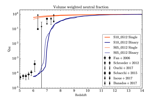
Fig. 9 shows the redshift evolution of the volume-filling fraction of neutral hydrogen, , for the and cMpc wide volumes, with single and binary SED models. Black datapoints in the same plot show model-dependent observational estimates from Fan et al. (2006), Schroeder et al. (2012), Ouchi et al. (2017), Sobacchi & Mesinger (2015), Inoue et al. (2017), and Bañados et al. (2017). The single and binary SED models produce very different reionization histories. The volumes are only reionized at with the single stars SED, while they are completely reionized by with binaries included. Note that for each SED, the two different curves are not only for different volume sizes (and hence a different range of halo masses) but also for different DM mass resolution, so the results are robust to both these factors. In Appendix B we also show that these reionization histories are robust with respect to resolution only (i.e. not changing the volume size at the same time). This insensitivity to box size is in part due to our method for selecting initial conditions to minimise cosmic variance effects (see §2.2.1). It is also an indication that our volumes are mostly ionized by intermediate-mass haloes, i.e. in the mass range , since this is the mass range overlapping our two volumes (see Fig. 2).
Neither SED model produces a reionization history in perfect agreement with the observational limits, but it is compelling and reassuring that variations in state-of-the-art SED modelling produce reionization histories that bracket the observational limits, without any calibration in unresolved escape fractions.
Note that in order to produce the good agreement with observations of the stellar mass to halo mass, SFR to halo mass, and luminosity function, we artificially boost the rate of SN explosions by a factor of four compared to that derived from a Kroupa (2001) IMF. Without the factor four boost, our stellar masses and SFRs are systematically higher than observations by factors of a few, as shown in Appendix C. Likewise, the resulting luminosity function is far too shallow compared to observations. However, as we also show in Appendix C, our main results are surprisingly insensitive to the feedback calibration, with remarkably similar reionization histories produced with and without the SN boost, even if galaxy luminosities are vastly overestimated in the un-boosted SN case.
In Fig. 10, we plot the simulated redshift evolution of the volume averaged in ionized gas, selecting only cells with hydrogen ionized fraction . The photo-ionization rate fluctuates strongly at high redshift, due to the rates being extracted from a small number of ionized regions nearby or inside haloes. Thus is very sensitive the current SFR. Some such regions, dim yet ionized by previous star formation events, can easily be identified by matching the temperature and photo-ionization rate projections in Fig. 8. Over time, the number of ionized regions increases and the strength of the fluctuations decreases as the average becomes less sensitive to individual regions. Eventually the fluctuations disappear completely with binary stars as individual Hii bubbles merge and the radiation field in any location becomes a composite of all the sources in the volume. The photo-ionization rate slightly over-predicts observations at although this is expected since the box reionizes at a marginally higher redshift than observations suggest. For the single stars SED, the fluctuations remain until , since the volume is not fully reionized, and the average photo-ionization rate is clearly well below the observational estimates, as expected from the reionization history in Fig. 9.

We finally note that our use of the variable reduced speed of light leads to a few tens of percent (relative) over-predictions of the neutral fraction and under-predictions of the photo-ionization rate, compared to a full light speed, when the volume is fully ionized (see §2.4 and a full explanation in Ocvirk et al. (2018): when reionization is completed and the whole volume becomes optically thin, the photon density turns light-speed independent and hence both the photon flux and the photo-ionization rate become light-speed dependent). With the binary SED model, a full speed of light would thus bring us further away from the observational data in Figures 9 and 10.
3.3 Escape fractions for individual haloes
The variable speed-of-light approximation makes it difficult to estimate directly from the M1 radiation field, due to the different and untraceable delay times for photons to travel from their sources to a given distance. Therefore, we measure the instantaneous escape fractions in post-processing by tracing rays from all stellar sources. We calculate the optical depth to neutral hydrogen and helium, , along each ray until it exits the virial boundary of its parent halo. We then determine the escape fraction for the ray as . The net escape fraction from each stellar particle is then the average of rays with random directions, and the net escape fraction for a halo at a given time is the luminosity-weighted average for all stellar particles assigned to the halo. We assign each stellar particle to the closest (sub-)halo, using for each halo the weighted distance measurement , where is the distance of the star from the halo center. A star outside of any halo is not assigned and we do not assign to any sub-halo fully enclosed within of its parent halo (i.e. stars within such a sub-halo are assigned to its parent halo).
We have checked in a few outputs that casting rays per source gives relative differences in of less than percent, compared to the fiducial rays. Hence it is fully justified to use rays per source. Trebitsch et al. (2017a) showed that this method of tracing rays in postprocessing yields almost identical results as integrating the flux of M1 photons across the virial radius (with a constant light-speed) and comparing to the galaxy’s ionizing photon production rate. Note that all of our escape fractions are luminosity-weighted, meaning represents the average escape probability per ionizing photon, not per source.
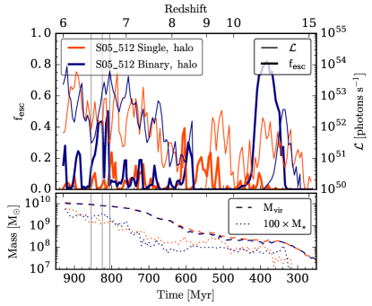

In Fig. 11 we compare the variation over time of from the most massive progenitor to the most massive halo at (, ) in the smaller-volume S05_512 simulations, with single and binary SED models (in red and blue, respectively). As found by Kimm & Cen (2014); Wise et al. (2014); Ma et al. (2016); Trebitsch et al. (2017a), the escape fraction varies strongly with time, due to regulation by SN feedback. Peaks in typically follow peaks in ionizing luminosity (denoted by thin curves) from bursty star formation events. The highly fluctuating nature of makes it difficult to compare the binary and stellar SED models for a single halo, but the plot shows generally higher for the binary SED, especially at late times.
To demonstrate how the variation is regulated by feedback, Fig. 12 shows neutral hydrogen column density and photo-ionization rate projections for the binary SED model at the three times, indicated by thin vertical lines at Myr in Fig. 11 (at this time, the virial mass of the halo is ). The left column corresponds to a peak of intrinsic ionizing luminosity, due to an ongoing starburst. The ISM of the galaxy is already quite disrupted but still intact enough that little of the ionizing radiation produced can escape. In the middle column, SN explosions have disrupted the ISM to the extent that star formation, and hence also the ionizing luminosity, is declining fast, but the more diffuse ISM now allows a significant fraction () of the ionizing photons to break out of the halo. In the right column, not much ionizing radiation comes from the galaxy because i) the ISM has settled back and is very low again and ii) the galaxy has become very faint in ionizing radiation due to the drop in star formation. This is a rather extreme example compared to most other peaks of in Fig. 11, but the picture is usually the same, with flashes of escaping ionizing radiation following star formation (and subsequent feedback) events. The first such event for the binary case in Fig. 11, at time Myr, is also the most extreme one in terms of duration and the peak value in . This is because, at this point, the system is very low in mass () and highly susceptible to disruption by SN feedback. This first strong starburst results in total obliteration of the ISM, so it takes more than a hundred million years to recover and start forming stars again.
3.4 Global escape fractions
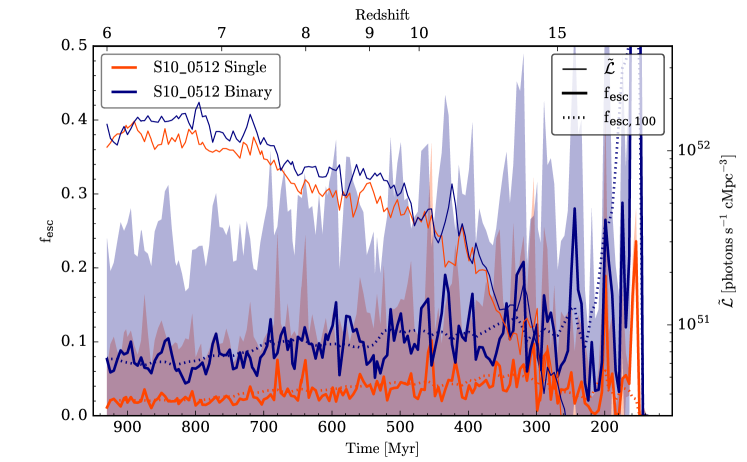
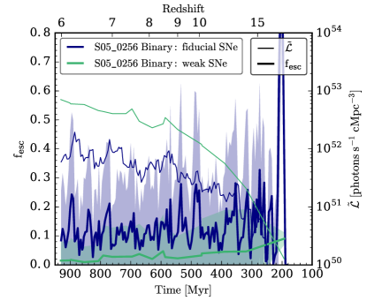
Fig. 13 shows the global luminosity-weighted for the cMpc volume, again for both the single and binary SED models, as well as the ionizing luminosities per volume (). We use the same definition for escape as in the previous section. We remind that we do not assign particles outside the of any halo, but note that such unassigned stellar particles account for less than percent of the total ionizing luminosity and hence their inclusion would have no effect on our estimated escape fractions.
Since the escape fraction is now averaged over a few thousand galactic sources, the fluctuations are not as extreme as seen in individual haloes, except at high redshift, when is dominated by a small number of galaxies. This makes it easier to compare the single- and binary-star SED models. In order to make the comparison even clearer, we plot in dotted curves the -weighted average over the last Myr, or . We show also the luminosity-weighted variance in the instantaneous , which is indicated with shaded regions. Note the distribution is highly non-gaussian and the variance here is meant only to give an indication of the range in that we measure at a given redshift.
For the binary SED model, the global escape fraction is at for , while for the single-star SED model it is at . In both cases there is a slight overall decline in with decreasing redshift. Sampled over every Myr until , the -weighted average is for binaries and for singles (i.e. times higher for binaries). This is in good agreement with Ma et al. (2016), who predict a factor of boost in ‘true’ escape fractions (i.e. omitting an extra luminosity boost) with binaries.
The higher with binaries partially explains the much more efficient reionization with the binary SED model. However, as shown with thin curves in Fig. 13, the production rate per volume of ionizing photons, , is also somewhat higher for the binary SED model. It is the combination of higher escape fractions and higher ionizing luminosities that leads to earlier reionization with binary stars. However, since the ratio of escape fractions between the single and binary SED models (a factor few) is consistently and significantly higher than the ratio of luminosities for those same models (typically a few tens of percent), we can conclude, as did Ma et al. (2016), that the higher dominates over the higher integrated luminosity with binary stars (seen in the lower panel of Fig. 3).

We further examine the variation in in Fig. 14, where we plot the luminosity-weighted probability distribution of escape fractions from all (halo-assigned) stellar particles at selected redshifts in our cMpc wide volume, with binary and single stars. The distribution peaks at zero or near-zero , as expected, but for higher there are a few non-systematic bumps in each snapshot. The reason for these bumps is that a few galaxies in each snapshot exist in the luminous and optically thin phase (similar to the middle column in Fig. 12). In this phase, the majority of young stars are exposed to the same low column density channels where a fixed fraction of the ionizing radiation can escape. In contrast, other stars are embedded in high density regions with negligible escape fractions (see also Cen & Kimm, 2015; Trebitsch et al., 2017a). Such a galaxy typically has a bi-modal distribution in : we include an example of this in the light-blue curve in Fig. 14, which shows the distribution from the massive halo in the S05_512_Binary simulation at a time of high (corresponding to the blue peak at Myr in Fig. 11). The series of bumps in Fig. 14 represent the rare luminous galaxies with high , each having a bi-modal distribution, while most galaxies at a given time either have a low and contribute mostly to the peak at , or they have a low luminosity and hence contribute little to the luminosity-weighted distributions plotted in Fig. 14. With larger simulation volumes, these bumps would presumably merge into a smooth distribution with a single peak at .
4 Discussion
With the Sphinx simulations, we find a significant boost in escape fractions with a SED model that includes binary stars, increasing to percent escape probability per photon from percent without the binaries. With the binary SED model, the volumes are also fully reionized at , even somewhat prematurely compared to observational constraints.
This puts our results in mild tension with estimations that a global is required to match observational constraints on reionization (e.g. Kuhlen & Faucher-Giguere, 2012; Ouchi et al., 2017). These estimates, however are based on simple analytic models for the competition between photo-ionization and recombination that depend on the clumping factor of gas in the IGM and the intrinsic ionizing luminosity density in the early Universe, in addition to . Neither of these two additional parameters are currently well constrained777Also, the Thompson optical depth Kuhlen & Faucher-Giguere (2012) calibrated their results against was a bit higher () than the current estimate () by Planck., so our is no cause for concern.
However, our results show a degeneracy between the efficiency of feedback and the reionization history, which is a natural outcome of the regulation by feedback, and does appear to generate some spread in the predicted . In Appendix C we show that significantly weaker SN feedback produces very similar reionization histories as our fiducial strong SN feedback, even if the rate of star formation, and hence the production of ionizing photons888There is not an exact linear relationship between the number of stars formed and the number of ionizing photons produced, since successive generations of stars have higher metallicities and hence lower luminosities (see Fig. 3). However, ten times more stars certainly produce many times more ionizing photons., is almost an order of magnitude higher.
This implies that the global escape fractions are significantly lower with weak feedback. In Fig. 15 we confirm this relationship between the strength of feedback and . The plot shows the global luminosity-weighted escape fractions and production rates of ionizing photons in our cMpc volume, with our fiducial rate of SNe and the four times lower SN rate directly derived from a Kroupa (2001) IMF. Indeed, the typical escape fraction with fiducial feedback, while highly fluctuating (due to the disrupting nature of strong feedback and small volume), is much higher than in the weak feedback case.
In §3.1 we show that even with our fiducial strong SN feedback, our galaxy stellar masses (Fig. 5) and luminosity function (Fig. 7) fall towards the upper end of observational constraints and recent models. The stellar masses can be lowered, via even stronger feedback, by roughly a factor of two and still be in good agreement with high-redshift observations and models. Based on our results with weaker feedback, such enhanced feedback simulations would likely result in similar reionization histories. Therefore, our model seems to allow for somewhat higher, but not lower, escape fractions, while still agreeing with observational constraints of the high- Universe.
Our results with binary stars, and in fact the actual event of reionization itself, appear to contradict observations of the low-redshift Universe (), where indirect measures have been made for the escape of ionizing photons from dwarf galaxies, resulting in upper limits of a few percent (e.g. Cowie et al., 2009; Bridge et al., 2010; Siana et al., 2010; Leitet et al., 2013). Reconciling this difference between low observationally estimated escape fractions at low redshift and relatively high escape fractions required to reionize the Universe is a well known puzzle which we will not solve in this paper. There are a few possible explanations that are exciting to explore in future work. Fig. 3 demonstrates that the decline in ionizing luminosity with stellar population age steepens with increasing metallicity. Similarly, the integrated ionizing luminosities mildly decrease with increasing metallicity. Both effects suggest a possible change in SEDs between high and low redshift. If dwarf galaxies become significantly and increasingly enriched, via long-term local star formation or external contamination (Anglés-Alcázar et al., 2017), their escape fractions may become very low as a result. Such a scenario, however, presents some tension with observations, as dwarf galaxies in the local Universe are not observed to become substantially enriched, with galaxies having th Solar metallicity (Kirby et al., 2013). The evolution in Fig. 14 of our Myr-averaged escape fraction, , does hint at the global escape fraction decreasing slowly over time, but confirming whether or not this is directly due to metallicity-dependence in the SED models is beyond the scope of this paper.
Another factor that may explain the low observed escape fractions is the stochastic nature of the escape of ionizing radiation from galaxies (Fig. 11, Kimm & Cen, 2014; Ma et al., 2016; Trebitsch et al., 2017a) which makes it very difficult to derive an average escape fraction with only a few observations. Based on a post-processing of the RHD simulation of Kimm & Cen (2014), Cen & Kimm (2015) indeed concluded that roughly galaxy spectra need to be stacked in order to draw meaningful conclusions on the average escape fraction.
Tempting as it is, we are reluctant to draw conclusions or preferences about different SED models from our results. Even if the two SED models we compare produce very different escape fractions and interestingly bracket current observational estimates of the reionization history, neither model produces a very good match with the observational data in Fig. 10. While this could be interpreted as some sort of uncertainty in SED models, it may just as well be a limitation of unresolved escape fractions. Presumably – and this will be attempted in future work – we could calibrate our unresolved escape fraction, with for the single-stars SED model and for the binary stars, and produce good matches with observations using either SED model. We cannot yet say for sure if the escape of radiation from the ISM is resolved in our simulations, nor can we tell whether it is over- or under-estimated, and hence it is not timely to rule out any SED models. We suffice to conclude that in the framework of our models, the inclusion of binary stars has a huge impact on the reionization history and makes it easy to reionize the Universe by .
We do not include active galactic nuclei (AGN) in our simulations, nor do we consider the effects of molecular cooling or POPIII stars. AGN are expected to become relevant in galaxies that are more massive those currently captured in our simulations (Trebitsch et al., 2017b; Mitchell et al., 2018). We aim in the next generation of larger-volume Sphinx simulations to study the possible contribution of more massive galaxies and AGN to reionization. However, their contribution to the EoR ionizing background is at best uncertain (see the debate in D’Aloisio et al., 2016; Chardin et al., 2016; Parsa et al., 2017). Regardless, the inclusion of binary stars in the emission from high-redshift stellar populations removes the need for any other sources of reionization than stars.
The possible contribution from metal-free (PopIII) stars has been considered in recent state-of-the-art models (Wise et al., 2014; Kimm et al., 2017) and the general conclusion is that they have relatively little direct impact on reionization at . The impact of PopIII stars during the EoR is an interesting question, but due to the large uncertainty in the PopIII initial mass function, a current inclusion of PopIII physics really constitutes an additional set of free parameters, which we prefer to skip in the first generation of our simulation suite.
For similar reasons of simplicity and transparency, we have chosen to not model the formation and destruction of molecular hydrogen. The first generation of stars was made possible by primordial molecular hydrogen formation and cooling, while successive generations formed via more efficient gas cooling catalysed by metals. In the current Sphinx simulations, instead of modeling the complex molecular hydrogen formation channels, we have imitated the effects of primordial molecular hydrogen by calibrating the initial gas metallicity in our simulations to reach a similar initial epoch and efficiency of star formation as in zoom-simulations where primordial molecular hydrogen formation was included (using the models described in Kimm et al., 2017).
5 Conclusions
This paper describes the Sphinx suite of cosmological simulations, the first non-zoom radiation-hydrodynamical simulations of reionization that capture the large-scale reionization process and simultaneously start to predict the escape fraction, , of ionizing radiation from thousands of galaxies. Our series of and co-moving Mpc wide volumes resolve haloes down to the atomic cooling limit and model the inter-stellar medium of galaxies with pc resolution. We select our cosmological initial conditions out of candidates to minimise the impact of cosmic variance on the volume-emissivity of ionizing photons and to maintain consistent reionization histories across different volumes.
Owing to strong SN feedback, our haloes are in good agreement with high-redshift observations, as well as recent state-of-the-art models, of the stellar mass to halo mass, star formation rate versus halo mass, and, most importantly, the Å UV luminosity function at (Fig. 7).
We study the effect of binary stars on reionization. Due to mass transfer and mergers between binary companion stars, spectral energy distribution (SED) models that include binary stars predict higher integrated ionizing luminosities for stellar populations as well as a much shallower decline of luminosity with stellar age (Stanway et al., 2016). We run and compare two sets of Sphinx simulations: one with the Bpass SED model (Eldridge et al., 2007) that includes binary stars, and one with the Bruzual & Charlot (2003) model, which does not. Using the M1 moment method for radiative transfer, we inject into our volumes the exact ionizing luminosities dictated by those SED models, given the metallicity, age, and mass of each stellar population particle, and without any calibration in unresolved escape fractions.
The reionization histories strongly differ in the models with and without binary stars (Fig. 9). The different reionization histories bracket the observed constraints, with the binaries model reionizing at , slightly earlier than observations predict, while the model with single stars does not ionize the volume by .
Because the escape fraction is regulated by feedback, as was demonstrated by Kimm et al. (2017) and later by Trebitsch et al. (2017a), it fluctuates strongly with time in an individual galaxy (Fig. 11), with brief flashes of radiation during which the galaxy satisfies the two conditions of being luminous and having an ISM disrupted enough for ionizing radiation to escape. The binary SED model consistently results in (luminosity-weighted) mean , with a large scatter. This is a factor higher than that for the singles-only SED model (Fig. 13).
The higher escape fractions are due to the combination of feedback and the shallower decline in stellar luminosities with binaries: by disrupting the ISM and clearing away dense gas, feedback simultaneously suppresses star formation and increases the local . With binary stars, more photons can escape, and for a longer time, after this ISM disruption, leading to larger globally averaged escape fractions. The higher escape fractions are the primary reason for the much earlier reionization with binaries, but the higher integrated luminosity with binaries also plays a sub-dominant role.
Our reionization histories are robust to changes in resolution, volume size, and, surprisingly, to changes in the SN feedback efficiency. The robustness to SN feedback is an outcome of an apparent balance between ionizing luminosities and escape fractions, which scale down and up, respectively, with increased feedback efficiency (Fig. 15).
We will follow up this work with an analysis of how escape fractions vary with halo mass and how haloes of different masses contribute to reionization. We will also use the Sphinx simulations to study the back-reaction of suppressed galaxy growth via reionization and to predict the observational properties of extreme-redshift galaxies, which will become increasingly visible to us when the JWST comes online.
Acknowledgements
We are grateful the reviewer, John Wise, for comments that strengthened the paper. We thank Dominique Aubert, Leindert Boogaard, Julien Devriendt, Yohan Dubois, Peter Mitchell, Ali Rahmati, Benoit Semelin, and Maxime Trebitsch for useful discussions, and Andreas Bleuler for very useful contributions to the optimisation of Ramses-RT. JR and JB acknowledge support from the ORAGE project from the Agence Nationale de la Recherche under grant ANR-14-CE33-0016-03. HK thanks the Beecroft fellowship, the Nicholas Kurti Junior Fellowship, and Brasenose College. TK is supported by the National Research Foundation of Korea to the Center for Galaxy Evolution Research (No. 2017R1A5A1070354) and in part by the Yonsei University Future-leading Research Initiative of 2017 (RMS2-2017-22-0150). TG is grateful to the LABEX Lyon Institute of Origins (ANR-10-LABX-0066) of the Université de Lyon for its financial support within the program “Investissements d’Avenir” (ANR-11-IDEX-0007) of the French government operated by the National Research Agency (ANR). Support by ERC Advanced Grant 320596 “The Emergence of Structure during the Epoch of reionization” is gratefully acknowledged. The results of this research have been achieved using the PRACE Research Infrastructure resource SuperMUC based in Garching, Germany. We are grateful for the excellent technical support provided by the SuperMUC staff. Preparations and tests were also performed at the Common Computing Facility (CCF) of the LABEX Lyon Institute of Origins (ANR-10-LABX-0066), and on the GENCI national computing centers at CCRT and CINES (DARI grant number x2016047376).
References
- Anglés-Alcázar et al. (2017) Anglés-Alcázar D., Faucher-Giguère C.-A., Kereš D., Hopkins P. F., Quataert E., Murray N., 2017, MNRAS, 470, 4698
- Aubert et al. (2004) Aubert D., Pichon C., Colombi S., 2004, MNRAS Letters, 352, 376
- Bañados et al. (2017) Bañados E. et al., 2017, Nature
- Behroozi et al. (2013) Behroozi P. S., Wechsler R. H., Conroy C., 2013, Astrophys. J., 770, 57
- Blondin et al. (1998) Blondin J. M., Wright E. B., Borkowski K. J., Reynolds S. P., 1998, Astrophys. J., 500, 342
- Bonazzola et al. (1987) Bonazzola S., Falgarone E., Heyvaerts J., Perault M., Puget J. L., 1987, Astron. Astrophys., 172, 293
- Booth et al. (2013) Booth C. M., Agertz O., Kravtsov A. V., Gnedin N. Y., 2013, Astrophys. J. Lett., 777, L16
- Bouwens et al. (2015) Bouwens R. J. et al., 2015, Astrophys. J., 803
- Bouwens et al. (2017) Bouwens R. J., Oesch P. A., Illingworth G. D., Ellis R. S., Stefanon M., 2017, Astrophys. J., 843, 129
- Bridge et al. (2010) Bridge C. R. et al., 2010, Astrophys. J., 720, 465
- Bruzual & Charlot (2003) Bruzual G., Charlot S., 2003, MNRAS Letters, 344, 1000
- Calverley et al. (2010) Calverley A. P., Becker G. D., Haehnelt M. G., Bolton J. S., 2010, MNRAS, 412, 2543
- Cen & Kimm (2015) Cen R., Kimm T., 2015, Astrophys. J. Lett., 801, L25
- Chardin et al. (2016) Chardin J., Puchwein E., Haehnelt M. G., 2016, Mon. Not. R. Astron. Soc. Vol. 465, Issue 3, p.3429-3445, 465, 3429
- Chen et al. (2017) Chen P., Norman M. L., Xu H., Wise J. H., 2017, eprint arXiv:1705.00026
- Commerçon et al. (2014) Commerçon B., Debout V., Teyssier R., 2014, Astron. Astrophys., 563, 11
- Cowie et al. (2009) Cowie L. L., Barger A. J., Trouille L., 2009, Astrophys. J., 692, 1476
- D’Aloisio et al. (2018) D’Aloisio A., McQuinn M., Davies F. B., Furlanetto S. R., 2018, MNRAS, 473, 560
- D’Aloisio et al. (2016) D’Aloisio A., Sanderbeck P. R. U., McQuinn M., Trac H., Shapiro P. R., 2016, MNRAS, 468, 4691
- Devriendt (2018) Devriendt J., 2018, in preparation
- Dijkstra & Loeb (2009) Dijkstra M., Loeb A., 2009, MNRAS Letters, 396, 377
- Eldridge et al. (2007) Eldridge J. J., Izzard R. G., Tout C. A., 2007, MNRAS, 384, 1109
- Fan et al. (2006) Fan X., Carilli C. L., Keating B., 2006, Annu. Rev. Astron. Astrophys., 44, 415
- Federrath & Klessen (2012) Federrath C., Klessen R. S., 2012, Astrophys. J., 761, 156
- Ferland et al. (1998) Ferland G. J., Korista K. T., Verner D. A., Ferguson J. W., Kingdon J. B., Verner E. M., 1998, Publ. Astron. Soc. Pacific, 110, 761
- Finlator et al. (2011) Finlator K., Dave R., Ozel F., 2011, Astrophys. J., 743, 169
- Gatto et al. (2016) Gatto A. et al., 2016, MNRAS, 466, 1903
- Geen et al. (2015) Geen S., Rosdahl J., Blaizot J., Devriendt J., Slyz A., 2015, MNRAS, 448, 3248
- Girichidis et al. (2016) Girichidis P. et al., 2016, Astrophys. J. Lett., 816, L19
- Gnedin (2014) Gnedin N. Y., 2014, Astrophys. J., 793
- Gnedin (2016) Gnedin N. Y., 2016, Astrophys. J., 833, 66
- Gnedin & Fan (2006) Gnedin N. Y., Fan X., 2006, Astrophys. J., 648, 1
- Gnedin & Kaurov (2014) Gnedin N. Y., Kaurov A. A., 2014, Astrophys. J., 793
- Guillet & Teyssier (2011) Guillet T., Teyssier R., 2011, J. Comput. Phys., 230, 4756
- Haardt & Madau (1996) Haardt F., Madau P., 1996, Astrophys. J., 461, 20
- Hahn & Abel (2011) Hahn O., Abel T., 2011, MNRAS, 415, 2101
- Hanasz et al. (2013) Hanasz M., Lesch H., Naab T., Gawryszczak A., Kowalik K., Wóltański D., 2013, Astrophys. J. Lett., 777, L38
- Harikane et al. (2017) Harikane Y. et al., 2017, eprint arXiv:1704.06535
- Hopkins et al. (2014) Hopkins P. F., Kereš D., Oñorbe J., Faucher-Giguère C.-A., Quataert E., Murray N., Bullock J. S., 2014, MNRAS, 445, 581
- Hopkins et al. (2012) Hopkins P. F., Quataert E., Murray N., 2012, MNRAS, 421, 3522
- Iliev et al. (2013) Iliev I. T., Mellema G., Ahn K., Shapiro P. R., Mao Y., Pen U.-L., 2013, MNRAS, 439, 725
- Inoue et al. (2017) Inoue A. K. et al., 2017, eprint arXiv:1801.00067
- Katz et al. (2018) Katz H., Kimm T., Haehnelt M., Sijacki D., Rosdahl J., Blaizot J., 2018, eprint arXiv:1802.01586
- Katz et al. (2017) Katz H., Kimm T., Sijacki D., Haehnelt M. G., 2017, MNRAS, 468, 4831
- Katz et al. (1996) Katz N., Weinberg D. H., Hernquist L., 1996, Astrophys. J. Suppl. Ser., 105, 19
- Kim & Ostriker (2015) Kim C.-G., Ostriker E. C., 2015, Astrophys. J., 802, 99
- Kimm & Cen (2014) Kimm T., Cen R., 2014, Astrophys. J., 788, 121
- Kimm et al. (2015) Kimm T., Cen R., Devriendt J., Dubois Y., Slyz A., 2015, MNRAS, 451, 2900
- Kimm et al. (2016) Kimm T., Cen R., Rosdahl J., Yi S. K., 2016, Astrophys. J., 823, 52
- Kimm et al. (2018) Kimm T., Haehnelt M., Blaizot J., Katz H., Michel-Dansac L., Garel T., Rosdahl J., Teyssier R., 2018, MNRAS, 475, 4617
- Kimm et al. (2017) Kimm T., Katz H., Haehnelt M., Rosdahl J., Devriendt J., Slyz A., 2017, MNRAS, 652, 4826
- Kirby et al. (2013) Kirby E. N., Cohen J. G., Guhathakurta P., Cheng L., Bullock J. S., Gallazzi A., 2013, Astrophys. J., 779
- Kroupa (2001) Kroupa P., 2001, MNRAS Letters, 322, 231
- Kuhlen & Faucher-Giguere (2012) Kuhlen M., Faucher-Giguere C.-A., 2012, Mon. Not. R. Astron. Soc, 423, 862
- Leitet et al. (2013) Leitet E., Bergvall N., Hayes M., Linné S., Zackrisson E., 2013, Astron. Astrophys., 553
- Levermore (1984) Levermore C. D., 1984, J. Quant. Spectrosc. Radiat. Transf., 31, 149
- Livermore et al. (2016) Livermore R. C., Finkelstein S. L., Lotz J. M., 2016, Astrophys. J., 835
- Ma et al. (2017) Ma X. et al., 2017, eprint arXiv:1706.06605
- Ma et al. (2016) Ma X., Hopkins P. F., Kasen D., Quataert E., Faucher-Giguere C.-A., Keres D., Murray N., Strom A., 2016, MNRAS, 459, 3614
- Martizzi et al. (2015) Martizzi D., Faucher-Giguère C.-A., Quataert E., 2015, MNRAS, 450, 504
- Mitchell et al. (2018) Mitchell P. D., Blaizot J., Devriendt J., Kimm T., Michel-Dansac L., Rosdahl J., Slyz A., 2018, MNRAS, 474, 4279
- Ocvirk et al. (2018) Ocvirk P., Aubert D., Deparis N., Lewis J., 2018, eprint arXiv:1803.02434
- Ocvirk et al. (2015) Ocvirk P. et al., 2015, MNRAS, 463, 1462
- Oke & Gunn (1983) Oke J. B., Gunn J. E., 1983, Astrophys. J., 266, 713
- Ouchi et al. (2017) Ouchi M. et al., 2017, eprint arXiv:1704.07455
- Pakmor et al. (2016) Pakmor R., Pfrommer C., Simpson C. M., Springel V., 2016, Astrophys. J., 824, L30
- Parsa et al. (2017) Parsa S., Dunlop J. S., McLure R. J., 2017, MNRAS, 474, 2904
- Pawlik et al. (2016) Pawlik A. H., Rahmati A., Schaye J., Jeon M., Vecchia C. D., 2016, MNRAS, 466, 960
- Planck Collaboration (2014) Planck Collaboration, 2014, Astron. Astrophys., 571, A1
- Rasera & Teyssier (2006) Rasera Y., Teyssier R., 2006, Astron. Astrophys. (ISSN 0004-6361), 445, 1
- Read et al. (2017) Read J. I., Iorio G., Agertz O., Fraternali F., 2017, MNRAS, 467, 2019
- Rosdahl et al. (2013) Rosdahl J., Blaizot J., Aubert D., Stranex T., Teyssier R., 2013, MNRAS, 436, 2188
- Rosdahl et al. (2017) Rosdahl J., Schaye J., Dubois Y., Kimm T., Teyssier R., 2017, MNRAS, 466, 11
- Rosdahl et al. (2015) Rosdahl J., Schaye J., Teyssier R., Agertz O., 2015, MNRAS, 451, 4553
- Rosdahl & Teyssier (2015) Rosdahl J., Teyssier R., 2015, MNRAS, 449, 4380
- Rosen & Bregman (1995) Rosen A., Bregman J. N., 1995, Astrophys. J., 440, 634
- Safarzadeh & Scannapieco (2016) Safarzadeh M., Scannapieco E., 2016, Astrophys. J. Lett., 832
- Schroeder et al. (2012) Schroeder J., Mesinger A., Haiman Z., 2012, MNRAS, 428, 3058
- Shull & van Steenberg (1985) Shull J. M., van Steenberg M. E., 1985, Astrophys. J., 298, 268
- Siana et al. (2010) Siana B. et al., 2010, Astrophys. Journal, Vol. 723, Issue 1, pp. 241-250 (2010)., 723, 241
- Smith et al. (2016) Smith A., Bromm V., Loeb A., 2016, MNRAS, 464, 2963
- So et al. (2013) So G. C., Norman M. L., Reynolds D. R., Harkness R. P., 2013, Astrophys. J., 789
- Sobacchi & Mesinger (2015) Sobacchi E., Mesinger A., 2015, MNRAS, 453, 1843
- Stanway et al. (2016) Stanway E. R., Eldridge J. J., Becker G. D., Z. H., D. M. T., N. K., Y. F., O. R., 2016, MNRAS, 456, 485
- Strömgren (1939) Strömgren B., 1939, Astrophys. J. Lett. v.489, 89, 526
- Teyssier (2002) Teyssier R., 2002, Astron. Astrophys., 385, 337
- Thompson et al. (2005) Thompson T. A., Quataert E., Murray N., 2005, Astrophys. J., 630, 167
- Thornton et al. (1998) Thornton K., Gaudlitz M., Janka H.-T., Steinmetz M., 1998, Astrophys. J., 500, 95
- Toro et al. (1994) Toro E. F., Spruce M., Speares W., 1994, Shock Waves, 4, 25
- Trebitsch et al. (2017a) Trebitsch M., Blaizot J., Rosdahl J., Devriendt J., Slyz A., 2017a, MNRAS, 470, 224
- Trebitsch et al. (2017b) Trebitsch M., Volonteri M., Dubois Y., Madau P., 2017b, eprint arXiv:1712.05804
- Tweed et al. (2009) Tweed D., Devriendt J., Blaizot J., Colombi S., Slyz A., 2009, Astron. Astrophys. (ISSN 0004-6361), 506, 647
- Verner et al. (1996) Verner D. A., Ferland G. J., Korista K. T., Yakovlev D. G., 1996, Astrophys. J. v.465, 465, 487
- Westera et al. (2002) Westera P., Lejeune T., Buser R., Cuisinier F., Bruzual G., 2002, Astron. Astrophys., 381, 524
- Wise & Cen (2009) Wise J. H., Cen R., 2009, Astrophys. J. Lett., 693, 984
- Wise et al. (2014) Wise J. H., Demchenko V. G., Halicek M. T., Norman M. L., Turk M. J., Abel T., Smith B. D., 2014, MNRAS, 442, 2560
- Wyithe & Bolton (2010) Wyithe S., Bolton J. S., 2010, Mon. Not. R. Astron. Soc. Vol. 412, Issue 3, pp. 1926-1936., 412, 1926
- Xu et al. (2016) Xu H., Wise J. H., Norman M. L., Ahn K., O’Shea B. W., 2016, Astrophys. J., 833
Appendix A Luminosity functions
For future comparisons to models and/or observations, we show in Table 4 our predicted Å luminosity functions for our and cMpc wide volumes, with the binary SED, at , and . These luminosity functions are also plotted in Fig. 16
| -20.5 | 0 | 0 | 0 | 0.001 | 0 | 0.001 |
|---|---|---|---|---|---|---|
| -19.5 | 0 | 0 | 0 | 0.001 | 0 | 0.001 |
| -18.5 | 0 | 0.001 | 0 | 0.004 | 0.008 | 0.01 |
| -17.5 | 0 | 0.004 | 0 | 0.012 | 0.008 | 0.017 |
| -16.5 | 0.008 | 0.012 | 0.032 | 0.023 | 0.032 | 0.05 |
| -15.5 | 0.016 | 0.034 | 0.56 | 0.068 | 0.096 | 0.106 |
| -14.5 | 0.048 | 0.083 | 0.104 | 0.124 | 0.168 | 0.159 |
| -13.5 | 0.160 | 0.140 | 0.264 | 0.235 | 0.256 | 0.306 |
| -12.5 | 0.256 | 0.242 | 0.472 | 0.374 | 0.496 | 0.486 |
| -11.5 | 0.488 | 0.344 | 1.096 | 0.514 | 1.072 | 0.674 |
| -10.5 | 0.816 | 0.421 | 1.496 | 0.678 | 1.784 | 0.909 |
| -9.5 | 0.744 | 0.385 | 1.640 | 0.728 | 2.728 | 1.147 |
| -8.5 | 0.776 | 0.441 | 1.880 | 0.954 | 3.176 | 1.52 |
| -7.5 | 0.800 | 0.394 | 1.944 | 0.993 | 3.712 | 1.907 |
| -6.5 | 0.224 | 0.168 | 1.136 | 0.616 | 3.448 | 1.685 |
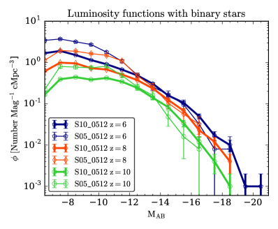
Appendix B Resolution convergence
In this Appendix we compare the main results of our fiducial simulations to those acquired with lower resolution, in order to show that they are not significantly affected by minor variations in spatial and mass resolution.
Fig. 17 shows the stellar mass to halo mass relation for resolution variations in our cMpc volume (with the binary SED model). The thickest (blue) curve shows our high-resolution case, where the DM mass resolution is and the maximum physical resolution at is pc. The medium-thickness (red) curve represents a run with our fiducial mass resolution, where the DM mass resolution is degraded to per DM particle, but the stellar mass and physical resolution remain fixed. The thinnest (green) curve represents another run where we have also degraded the maximum physical resolution, which is now at pc at . These resolution changes have little and non-systematic effects on the stellar mass to halo mass relation. The most noticeable difference is a hint of systematically higher stellar mass for the most massive haloes with degraded physical resolution, but this may as well be due to low number statistics.
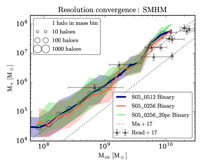
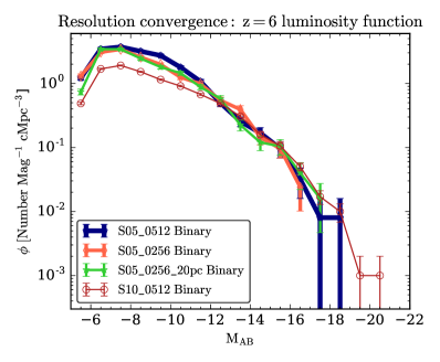
We show how the luminosity function for the cMpc volume changes with resolution in Fig. 18. There is little systematic difference for the different resolution runs, except for a hint of slightly more galaxies at the faint end with higher DM mass resolution. Comparing with the larger volume (shown in red) the luminosity function is clearly much more sensitive to the cosmological initial conditions than to factor-few changes in resolution. From Fig. 7 it is also clear that using different SED models has a larger effect than those resolution changes. There are, however, likely stellar mass resolution effects at the low-luminosity end, manifested in the down-turn in the luminosity functions in the faintest bin. Our galaxies with contain fewer than stellar particles on average: their star formation histories are overly discrete and likely underestimated.
In Fig. 19 we show how the same variations in resolution affect the reionization history. The aforementioned variations in resolution have minor effects on the reionization history which do not appear to be systematic. These minor variations in the evolution are likely the result of the stochasticity of starbursts and feedback in our relatively small simulation volume in the calibration simulations. We can confirm that simply varying the random seeds for star formation has similar-amplitude effects on the reionization history as these resolution variations.
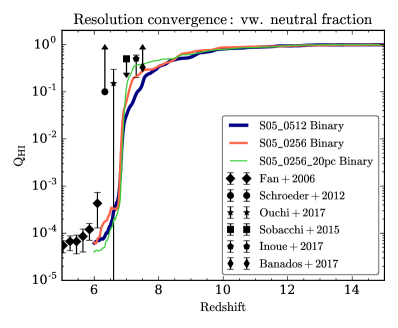
Note that we have not studied a degraded stellar mass resolution. We expect that variations in the stellar mass resolution within sensible limits has little effect, since we inject individual SN explosions rather than instantaneously injecting the total SN energy for the mass of each stellar population particle (the latter would translate into stronger resolution effects, with fewer, more energetic SN explosions). Furthermore, decreasing the stellar particle mass significantly from our brings us into a questionable regime where the IMF is no longer sampled by a single particle and we need to consider more sophisticated models for stellar populations.
Appendix C Calibration of SN feedback
We now demonstrate how our SN feedback model is calibrated to match constraints to the Å UV luminosity function and the SMHM relation.
In Fig. 20 we compare simulated Å luminosity functions at in our cMpc volume (with fiducial resolution) with observations from Bouwens et al. (2017) and Livermore et al. (2016). The thin green curve shows the luminosity function for an uncalibrated SN rate derived from a Kroupa (2001) IMF, with type II SN explosions per . The thick blue curve shows the results for our fiducial SN feedback, where the rate of SN explosions has been boosted four-fold, so that SN explosions occur per . Both are run with the binary SED model (which is also used to calculate the luminosity of each galaxy; as usual dust attenuation is ignored). The lower SN rate is clearly insufficient to produce a realistic luminosity function, while the fiducial boosted feedback produces a luminosity function in reasonable agreement with the observational constraints. As we have seen in Fig. 7, this agreement for the fiducial calibrated SN feedback, holds both in the case of higher mass resolution and for an eight times larger volume.
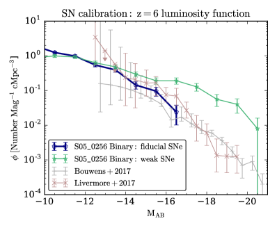
Fig. 21 shows a comparison, for the same two simulations, of the predicted SMHM relation. We include the local Universe observations from Read et al. (2017) and the relation derived by Behroozi et al. (2013). Our fiducial SN feedback results in a SMHM relation that agrees well with local Universe observations and does not appear in conflict with high-z constraints. The uncalibrated feedback produces much higher stellar masses, by almost an order of magnitude at the high-mass end.

Our fiducial four-fold boost in the rate of SN explosions is a simple substitute for an unknown combination of the following and possibly incomplete list of factors: i) uncertainty in the IMF and hence the rate of SN explosions. ii) resolution, which may play a role, but likely not a large one, as our resolution has been demonstrated to produce results that are resolution-converged and not subject to severe over-cooling. iii) uncertainty in gas cooling rates, which affects the final momentum gained in the remnants of SN explosions. iv) lack of complementary feedback physics, such as cosmic rays, stellar winds, or active galactic nuclei, though the latter is unlikely in the mass range for galaxies captured in our simulations (Trebitsch et al., 2017b).
Regardless, our main result – of a large difference in the reionization histories produced by single and binary stellar populations – is robust with respect to the feedback calibration. Fig. 22 shows that the reionization histories are very similar if the feedback is not boosted, and the same difference remains between single and binary stellar populations. It may seem counter-intuitive that reionization progresses as efficiently with weak SN feedback, but this is due to the feedback regulation of both star formation and . Many more stars are produced with the weaker feedback model and this leads to larger ionizing luminosities. However, the SNe also become less efficient at disrupting the ISM, leading to a smaller fraction of photons which escape into the IGM. With the higher luminosities but lower escape fractions, a comparable number of ionizing photons escapes the galaxies compared to our fiducial model,
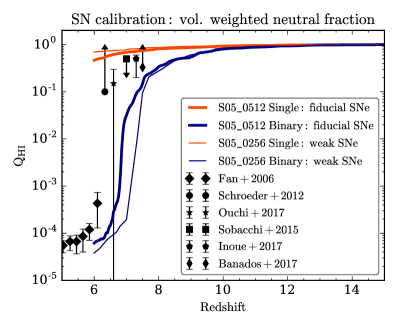
Appendix D SED properties
The ionizing luminosities of stellar particles in our simulations, as well as the properties of the three radiation groups, are based on two spectral energy distribution (SED) models, which each provide a set of spectra binned by metallicity and population age (assuming an instantaneous formation time), and normalised to .
One set of simulations uses Bruzual & Charlot (2003) (BC03), which includes only single star systems. Here, we use the model generated with the semi-empirical BaSeL 3.1 stellar atmosphere library (Westera et al., 2002) and a Kroupa (2001) initial mass function (IMF). The other set of simulations uses the Bpass model (Eldridge et al., 2007), which includes binary stars, and has an IMF closest to Kroupa (2001), with slopes of from to and from to . Fig. 23 shows in detail the age- and metallicity-dependency of the stellar population luminosities, number weighted mean photon energies, and cross sections, for all three radiation groups (defined in Table 3), integrated from the two SED spectra for bins of population age and metallicity.
From each SED spectrum (in units of ), we extract and tabulate age- and metallicity-dependent ionising luminosities, average energies, number-, and energy-weighted cross sections for all radiation groups, by integrating over the wavelength interval defined for each group.999For BC03, the ages range from zero to Gyr, and for BPASS from zero to 20 Gyr. The metallicities range from for BC03 and for BPASS. Using linear interpolation, we then re-bin the tables in age and metallicity (8 bins) so that the increment is linear in log-space, i.e. is the same for every age-interval (giving 266 bins for BC03, 209 bins for BPASS) and ( for BC03, for BPASS) is the same for every metallicity-interval. The purpose of the re-binning is to speed up the age- and metallicity-interpolation performed for every star particle in every RHD time-step. The lowest tabulated zero-age is a special case for the interpolation, since we cannot tabulate the logarithm of zero.
For each re-binned age bin, we integrate and tabulate the cumulative luminosity (number of photons per Solar mass emitted up to given age), assuming constant metallicity. We then use this re-binned table to extract the number of photons emitted by a stellar particle by comparing the cumulative luminosity before and after the RHD timestep. We use the cumulative luminosity rather than simply multiplying the instantaneous luminosity by the timestep length, because if the timestep happens to be very large, short bursts in luminosity may be lost entirely. Using the cumulative luminosity ensures that these unresolved bursts are still accounted for in the photon budget.
For metallicities outside the table limits, we use the lowest or highest tabulated metallicity (this is irrelevant for age, which is always within the tabulated limits). We feel this is a more conservative option than to apply extrapolation outside the metallicity limits: the BC03 model reaches ten times lower metallicity than BPASS, and lower metallicity generally leads to higher ionising luminosity (see Fig. 23). Hence, if there is an under-estimate of luminosities at very low metallicities due to our lack of extrapolation, the under-estimate should be more exaggerated with BPASS than with BC03, i.e. we are then underestimating the difference between BPASS and BC03.
Every ten coarse time-steps, we update the photo-ionization cross sections and energies for the radiation groups in our simulations, to represent the luminosity-weighted average of all emitting sources in our simulations. The details of this process are described in Appendix B2 in Rosdahl et al. (2013). Note that since stellar population particles have different ages and metallicities, and hence different spectra as defined by the assumed SED model, the emission of photons into a radiation group cannot be exactly energy-conserving and photon-number conserving at the same time. Given the energy per photon defined for the group, we can choose to emit either i) the exact amount of energy per time, leaving a small error in the number of photons per time, due to the difference in the particle spectrum over the group frequency interval from the ‘average’ group spectrum, or ii) the exact number of photons, sacrificing in the same way the exact energy luminosity. In this work, we have chosen the latter, as the number of ionizing photons is more important in the context of reionization.