LOOKING FOR A NEW TEST OF GENERAL RELATIVITY
IN THE SOLAR SYSTEM

Abstract

This paper discusses three matter-of-principle methods for measuring the general relativity correction to the Newtonian values of the position of collinear Lagrangian points $L_{1}$ and $L_{2}$ of the Sun-Earth-satellite system. All approaches are based on time measurements. The first approach exploits a pulsar emitting signals and two receiving antennas located at $L_{1}$ and $L_{2}$, respectively. The second method is based on a relativistic positioning system based on the Lagrangian points themselves. These first two methods depend crucially on the synchronization of clocks at $L_{1}$ and $L_{2}$. The third method combines a pulsar and an artificial emitter at the stable points $L_{4}$ or $L_{5}$ forming a basis for the positioning of the collinear points $L_{1}$ and $L_{2}$. Further possibilities are mentioned and the feasibility of the measurements is considered.

Received (Day Month Year)Revised (Day Month Year)

PACS Nos.: 04.20Cv, 95.10.Ce

1 Introduction

From the age of Laplace and Poincaré [1, 2, 3] until recent times [4, 5], celestial mechanics has played the crucial role of providing a testbed for the theories of gravitation that mankind has been able to develop. When Poincaré discovered chaos in his investigation of $3$-body dynamics in Newtonian gravity, he stressed this peculiar role of celestial mechanics at the beginning of his monumental treatise on the new methods of celestial mechanics [3]. A quarter of a century later, after Einstein arrived at his geometric view of gravitation, the precession of Mercury’s perihelion, observed by the astronomers, turned out to be in complete agreement with the calculation based upon the geodesic motion of planets in Einstein’s theory [6], and since then his general relativity has passed many observational tests [7], including the recent discovery of gravitational waves [8]. However, in the light of the accelerated expansion of the universe, which seems to cast doubts on the attractive nature of gravity on all scales, and bearing in mind the attempt to question the existence of dark matter by appealing to modified gravitational Lagrangians [9] (cf. Ref. [10]), satellite and planetary motions in the solar system are still receiving careful consideration, with the hope of being able to discriminate between Einstein’s theory and extended gravity theories [11, 12].

Over the last few years, some of us have looked, in particular, at the tiny corrections to the location of Lagrangian points, both stable and unstable, in the Earth-Moon-satellite [13, 14, 15, 16] and Sun-Earth-satellite [17] $3$-body systems. In the present letter we are concerned with the purely classical corrections that Einstein’s theory predicts for the location of collinear Lagrangian points, with respect to Newtonian gravity. We had originally looked at the Earth-Moon-satellite system, but the corresponding corrections are a few millimeters only. This theoretical value is conceptually interesting but is still too small, despite the extraordinary progress made by laser ranging techniques, that have reached the centimeter accuracy by now. Moreover, for the location of collinear Lagrangian points $L_{1}$ and $L_{2}$ of the Sun-Earth-satellite system, we have recently found that Einstein’s theory corrects Newtonian gravity by $5$ meters and $-4.8$ meters, respectively [17]. These corrections are apparently big enough to allow for experimental verification.

It is now our aim to discuss the possibility of measuring such an effect, which seems to be a good example of Galilean physics within mankind’s reach.

2 Approach (a): pulsars

Let us start from the work in Ref. [17], and in particular from Table 3 therein, which displays an important general relativistic correction to the location of collinear Lagrangian points $L_{1}$ and $L_{2}$ for a $3$-body system consisting of Sun, Earth and a satellite, with respect to the Newtonian gravity. The amount of the correction has been mentioned in the introduction; considering the effect on both $L_{1}$ and $L_{2}$, the two points turn out to be $9.8$ m closer to one another. We may think of detecting such change of distance between the two collinear points, at least in principle, by measuring the time of flight difference of an electromagnetic signal between $L_{1}$ and $L_{2}$.

In the first approach that we present, our idea it to use signals emitted from one or more pulsars (for redundancy). Once we have chosen a specific pulsar, suppose that two receiving antennas (radiotelescopes) are available, one at $L_{1}$ and the other at $L_{2}$. The wavefronts of the pulses emitted from the pulsar first run over $L_{2}$ then $L_{1}$ (or in the reverse order). The difference in the arrival times depends on the distance between the two points and on the angle $\alpha$ between the $L_{1}$-$L_{2}$ axis and the direction of the pulsar (assumed to be at infinity). The setting is shown in Fig. 1 below.

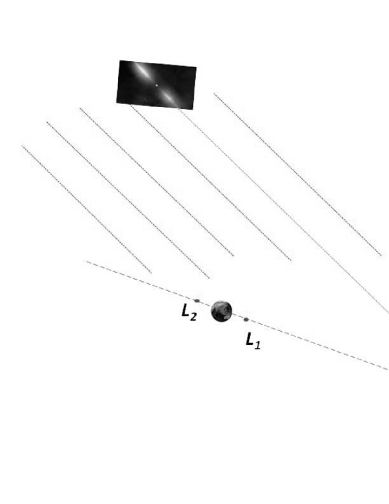
Figure 1: On top we represent the pulsar that emits signals, while $L_{1}$ and $L_{2}$ are two collinear Lagrangian points of the Sun-Earth-planetoid system, and $\alpha$ is the angle between the line joining such points and the direction of the pulsar.

On denoting by $a$ the distance between $L_{1}$ and $L_{2}$, the arrival times difference $\tau$ is

$$\tau={a\over c}\cos(\alpha).$$ (1)

The approximate value of $a$ is

$$a\approx 3\times 10^{9}\;{\rm m},$$ (2)

and hence

$$\tau\leq 10\;{\rm s}.$$ (3)

As we have already seen, according to Ref. [17], the general relativity correction to $a$ amounts to a variation $\delta a=9.8$ meters, which implies a relative variation

$${\delta a\over a}\approx 3\times 10^{-9}.$$ (4)

The resulting expected change in the times of arrival difference would be

$$\delta\tau\leq 3\times 10^{-8}\;{\rm s},$$ (5)

which means that the accuracy in the measurement of time should of course be better than that. Moreover, it implies that the Newtonian positions of collinear points $L_{1}$ and $L_{2}$ should be known with accuracies better than at least $1$ meter.

As far as the choice of the pulsar is concerned, one should look for a sufficiently bright one (although it is known that they are, in general, very faint objects). The available periods range from a few $ms$ to a few $s$, and the relative stability of the emission rate (rotation of the star) may be $1$ part in $10^{12}$ per cycle. Single pulses are usually not identical to one another, however, for the application we are considering here, what really matters is the possibility to recognize one and the same pulse after it has passed through the Lagrangian points $L_{1}$ and $L_{2}$.

In practice, one should record a sequence of pulses both at $L_{1}$ and at $L_{2}$, then the two series should be confronted in the same time reference and shifted until they coincide. The duration of the shift would measure the difference in the arrival times; it should be measured with an accuracy better at least than $10^{-8}$s, in order to make the comparison between the Newtonian and the general relativity results possible.

Of course, the measurement should be performed by considering a variety of sources with different positions in the sky and different periods. A non-trivial basic problem is that one should previously synchronize the clocks at $L_{1}$ and $L_{2}$ with an accuracy better than $1$ ns.

3 Approach (b): a relativistic positioning system based upon the Lagrangian points themselves

The Lagrangian points of the Sun-Earth-satellite $3$-body system are fit to be the material bases for a Relativistic Positioning System [18, 19]. However in this case the situation, by virtue of peculiar symmetries, looks simpler. All Lagrangian points lie in the same plane, and the two that are more interesting for us are located along the Sun-Earth line; in practice, the problem is therefore one-dimensional.

Suppose then to locate beacons at the stable points $L_{4}$ and $L_{5}$ emitting periodic signals at a stable frequency; they would act with respect to $L_{1}$ and $L_{2}$ more or less as artificial pulsars, with much stronger signals.

Apparently, only one emitter would be enough (either at $L_{4}$ or at $L_{5}$). The emission sequence from, say, the stable point $L_{4}$, since the emitter is at rest with respect to $L_{1}$ and $L_{2}$, coincides with the sequence of arrivals at $L_{1}$; the unstable point $L_{2}$ will receive the same sequence, with some delay depending on the greater distance of the receiver from the emitters. The procedure is then the same as for the pulsars in the previous section, and also for the accuracies involved the same considerations can be made. The difficulty that is challenging us is also the same: the clocks at collinear points $L_{1}$ and $L_{2}$ must be synchronous.

4 Approach (c): stable Lagrangian points and a pulsar

In order to avoid the need for synchronization of the clocks, the full Relativistic Positioning System should be used. In practice, at least one source of pulses out of the ecliptic plane is required, and this can be a pulsar. The pulsar and an artificial emitter at $L_{4}$ or $L_{5}$ can provide the positioning of unstable Lagrangian points $L_{1}$ and $L_{2}$ both in space and time, i.e. to give the relative distance between them.

As for the practical aspects of measurements as the ones we have suggested here, we must add that, of course, we would not have spacecrafts permanently located at $L_{1}$ and $L_{2}$. Both positions are indeed unstable, so that the receivers therein would move around the corresponding Lagrangian point along Lissajous orbits. Consequently the measurement should be repeated several times. The reference would then be to the average position over time, the center of the instantaneous positions being coincident with the Lagrangian point.

5 Closed contours

The difficulty of synchronizing clocks located million kilometers apart from one another is not easy to surmount. A way to solve the problem would be to use just one clock. This would be possible if the electromagnetic signals move along a closed path in space, starting from and arriving to the same position. Consider for instance a path $L_{1}-L_{4}-L_{2}-L_{5}-L_{1}$; its length (see fig. 2) would be

$$l=2\left(\sqrt{\Lambda^{2}+\Lambda a^{\prime\prime}+a^{\prime\prime 2}}+\sqrt{\Lambda^{2}-\Lambda a^{\prime}+a^{\prime 2}}\right).$$ (6)

With our notation, $\Lambda$ is the distance of $L_{4}$ or $L_{5}$ from the Earth and corresponds to $1$ AU; $a^{\prime}$ is the distance of $L_{1}$ from the Earth and $a^{\prime\prime}$ is the distance of $L_{2}$ from the Earth; of course $a^{\prime}+a^{\prime\prime}=a$.

On taking into account that $a^{\prime}\simeq a^{\prime\prime}\sim\frac{\Lambda}{10}$, the total time of flight of light moving along the path would be approximately $2000$ s. A change $\delta a$ of the distance $a$ would produce a time of flight change

$$\delta\tau\simeq 5\times 10^{-9}\;{\rm s}.$$ (7)

A more favorable configuration would be obtained by using the triangle $L_{2}-L_{5}-L_{4}-L_{2}$ (see fig. 2). In that case the total path would be $l=2\sqrt{\Lambda^{2}+a^{\prime\prime}\Lambda+a^{\prime\prime 2}}+\sqrt{3}\Lambda$; the corresponding time of flight is approximately $1920$ s, and the change in the time of flight induced by a change $\delta a^{\prime\prime}=5$ m would be roughly

$$\delta\tau\simeq 2\times 10^{-8}\;{\rm s}.$$ (8)

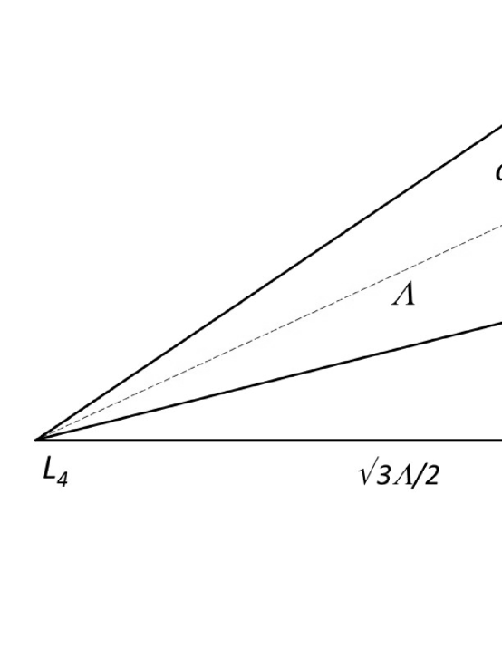
Figure 2: The scheme (not on scale) represents the possible closed paths including the Lagrangian points to be used to send electromagnetic signals and measure the times of flight along closed paths.

6 Discussion

The models we have considered have a matter-of-principle nature. A number of practical problems are however present. For example, as shown in detail by Brumberg, by virtue of the emission of gravitational radiation, the libration points $L_{1},L_{2},L_{3},L_{4},L_{5}$ of Newtonian theory are, strictly, quasi-libration points.[20] Moreover, non-gravitational perturbations must also be accounted for; for instance, radiation pressure affects the motion of a spacecraft,[21, 22, 23, 24, 25, 26] and hence a proposal to a space agency should consider carefully also the shape of the desired satellite, especially in the case that extended antennas should be deployed.

Leaving such complications aside, one can say what follows. So far, we have described our original ideas on how in principle the correction in the position of the Sun-Earth collinear Lagrange points, induced by General Relativity effects, could be measured. It is not the purpose of the present paper to enter a detailed technical analysis, but some comments on the practical feasibility and the problems to tackle are in order.

Let us start with the proposal to use pulsars, approach a of Sect. 2. As mentioned therein, a practical problem is the size of the required antenna, by virtue of the weakness of signals. It is worth mentioning a solution that would be viable: using X-ray pulsars. Such sources are much less numerous than the more common radio-pulsars, but the antennas they need have much smaller size than radiotelescopes. The use of X-ray pulsars is indeed under study and development by NASA for space navigation purposes (XNAV system); see for instance Ref. [27]

The other major delicate issue, besides the need for synchronization of the clocks, is the actual position of the spacecraft that should mark $L_{1}$ and $L_{2}$. Of course, they would move around the corresponding Lagrangian points, rather than stably stop there. As we said before, the position at collinear points is unstable and a station therein would move around the Lagrangian point, tracing planar Lissajous figures or halo orbits, with a period of approximately six months. The receiver would then slowly drift away. The whole issue is discussed in Sect. 6 of Ref. [19] Upon considering our approach (c), also $L_{4}$ or $L_{5}$ come into play and, of course, also for them the problem would arise of what is the actual position of the spacecraft while performing the measurement. Now the orbits are stable quasi-periodic, with a period of order one year.

Last but not least, the accuracy with which the Newtonian position of $L_{1}$ and $L_{2}$ can be calculated depends on the accuracy on the value of the masses of the Earth and the Sun, and on the distance between the two bodies. At the moment the resulting uncertainty in the position of the two $L$-points seems to be bigger than the correction due to General Relativity. Furthermore the orbit of the earth is not exactly circular, which means that the position of both $L_{1}$ and $L_{2}$ periodically changes during the year.

The above remarks tell us that we should in any case think of a measurement strategy where we look for the central values in a cloud of results generated by the instantaneous positions of the space stations (and even of the $L$-points). Taking into account the slowness of the movements about the Lagrangian points, the data acquisition should last quite a few years.

References

- [1] P. S. Laplace, Traité de Mécanique Céleste (Imprimerie Royale, Paris, 1843 to 1846)
- [2] F. F. Tisserand, Traité de Mécanique Céleste (Gauthier-Villars, Paris, 1889 to 1896).
- [3] H. Poincaré, Les Méthodes Nouvelles de la Mécanique Céleste (Gauthier-Villars, Paris, 1892 to 1899).
- [4] S. Kopeikin and I. Vlasov, Phys. Rep. 400, 209 (1994).
- [5] S. Kopeikin, M. Efroimsky and G. Kaplan, Relativistic Celestial Mechanics of the Solar System (Wiley, New York, 2011).
- [6] Y. Choquet-Bruhat, General Relativity and the Einstein Equations (Oxford University Press, Oxford, 2009).
- [7] C. M. Will, Theory and Experiment in Gravitational Physics, Second Edition (Cambridge University Press, Cambridge, 1994).
- [8] B. P. Abbott et al., Phys. Rev. Lett. 116, 061102 (2016).
- [9] S. Capozziello and M. De Laurentis, Phys. Rep. 509, 167 (2011).
- [10] R. An, C. Feng and B. Wang, arXiv:1711.06799 [astro-ph.CO].
- [11] M. Martini and S. Dell’Agnello, Probing gravity with next generation lunar laser ranging, in: Gravity: Where Do We Stand (Springer, 2016), pp. 195-210; ISBN 978-3-319-20224-2.
- [12] E. Ciocci et al., J. Adv. Space Res. 60, 1300 (2017).
- [13] E. Battista and G. Esposito, Phys. Rev. D 89, 084030 (2014).
- [14] E. Battista and G. Esposito, Phys. Rev. D 90, 084010 (2014).
- [15] E. Battista, S. Dell’Agnello, G. Esposito and J. Simo, Phys. Rev. D 91, 084041 (2015).
- [16] E. Battista, S. Dell’Agnello, G. Esposito, L. Di Fiore, J. Simo and A. Grado, Phys. Rev. D 92, 064045 (2015).
- [17] E. Battista, G. Esposito, L. Di Fiore, S. Dell’Agnello, J. Simo and A. Grado, Int. J. Geom. Methods Mod. Phys. 14, 1750117 (2017).
- [18] A. Tartaglia, M. L. Ruggiero and E, Capolongo, Adv. Space Res. 47, 645 (2011).
- [19] A. Tartaglia, E. Lorenzini, D. Lucchesi, G. Pucacco, M. L. Ruggiero and P. Valko, Gen. Relativ. Gravit. 50 (2018).
- [20] V. A. Brumberg, Cel. Mech. Dyn. Astr. 85, 269 (2003).
- [21] H. F. Fliegel, T. E. Gallini and E. R. Swift, J. Geophys. Res. 97, 559 (1992).
- [22] H. F. Fliegel and T. E. Gallini, J. Spacecraft & Rockets 33, 863 (1996).
- [23] P. Farinella and D. Vokrouhlicky, Planet. Space Sci. 44, 1551 (1996).
- [24] S. Adhya, Thermal Re-Radiation Modelling for the Precise Prediction and Determination of Spacecraft Orbits, Ph.D. Thesis, UCL London (2005).
- [25] J. Ray, Z. Altamimi, X. Collilieux and T. van Dam, GPS Solut. 12, 55 (2008).
- [26] C. J. Rodriguez-Solano, U. Hugentobler, P. Steigenberger and S. Lutz, J. Geodesy 86, 309 (2012).
- [27] https://www.nasa.gov/sites/default/files/atoms/files/session_3_-_2_x-ray_pulsar_navigation_for_deep-space_autonomous_applications_jason_mitchell_0.pdf