Medium-sized satellites of large Kuiper belt objects

Abstract

While satellites of mid- to small-Kuiper belt objects tend to be similar in size and brightness to their primaries, the largest Kuiper belt objects preferentially have satellites with small fractional brightness. In the two cases where the sizes and albedos of the small faint satellites have been measured, these satellites are seen to be small icy fragments consistent with collisional formation. Here we examine Dysnomia and Vanth, the satellites of Eris and Orcus, respectively. Using the Atacama Large Millimeter Array, we obtain the first spatially resolved observations of these systems at thermal wavelengths. Vanth is easily seen in individual images and we find a 3.5$\sigma$ detection of Dysnomia by stacking all of the data on the known position of the satellite. We calculate a diameter for Dysnomia of 700$\pm$115 km and for Vanth of 475$\pm$75 km, with albedos of 0.04${}^{+0.02}_{-0.01}$ and 0.08$\pm$0.02 respectively. Both Dysnomia and Vanth are indistinguishable from typical Kuiper belt objects of their size. Potential implications for the formation of these types of satellites are discussed.

1. Introduction

Most of largest objects in the Kuiper belt are known to have one or more satellites orbiting the parent body. The majority of these satellites have a small fractional brightness compared to their parent body. Even before the discovery of any of these small satellites, models predicted that giant impacts onto differentiated bodies would preferentially form icy satellites with a small fractional mass (Canup, 2005). Many of the known satellites to large Kuiper belt objects (KBOs) appear consistent with this paradigm. In the two cases where compositional information of these small satellites is available, these satellite surfaces are known to have a high albedo and to be dominated by water ice. The small satellites of Pluto have been directly imaged by the New Horizons spacecraft and have measured albedos of 0.5-0.9 and deep water ice absorptions in the near infrared (Weaver et al., 2016; Cook et al., 2017), while the satellites of Haumea show deep water ice absorption (Barkume et al., 2006; Fraser & Brown, 2009), and dynamical modeling strongly suggests low mass and thus high albedo (Ragozzine & Brown, 2009).

Little is known about the size or albedo of other satellites around large KBOs owing to the difficulty of resolving the satellites at anything other than optical or near-infrared wavelengths. The recently improved capability of the Atacama Large Millimeter Array (ALMA) to obtain spatial resolutions of 10s of milliarcseconds, however, allows us to now measure thermal emission directly from KBO satellites. Here, we use spatially resolved observations from ALMA to examine the size and albedo of two satellite systems: Eris-Dysnomia and Orcus-Vanth. Dysnomia, with a fractional brightness of 0.2% that of Eris (Brown & Schaller, 2007), appears to fit the paradigm of small, icy, collisionally-induced satellites surrounding all of the largest known dwarf planets (Brown et al., 2006; Parker et al., 2016; Kiss et al., 2017). A closer look at the system, however, makes this assessment less certain. The unusually high albedo of Eris of 0.97 (Sicardy, 2011) makes Dysnomia’s relative brightness seem artificially low. In fact, if Dysnomia has a typical small-KBO-like albedo of $\sim$5%, it is as large as 630 km. On the other hand, if Dysnomia has an icy-collisional-satellite like albedo of 0.5 or higher it is smaller than 200 km in radius. This range in sizes spans a wide range of the types of satellite systems in the Kuiper belt. Without a constraint on the size of Dysnomia, we lack a fundamental understanding of this system. A counter-example is the dwarf planet Orcus, which has a satellite – Vanth – with a fractional brightness of 9.6% and a spectrum with significantly less water ice than its primary (Brown et al., 2010). The origin of this type of dwarf planet system remains uncertain, with models from capture to collision being plausible (Ragozzine, 2009).

2. Observations

Observations of Orcus-Vanth and Eris-Dysnomia were undertaken with the 12-m array of the Atacama Large Millimeter Array (ALMA). This synthesis array is a collection of radio antennas, each 12 m in diameter, spread out on the Altiplano in the high northern Chilean Andes. Each of the pairs of antennas acts as a two element interferometer, and the combination of all of these individual interferometers allows for the reconstruction of the full sky brightness distribution, in both dimensions (Thompson et al., 2001).

ALMA is tunable in 7 discrete frequency bands, from $\sim$90 to $\sim$ 950 GHz. All observations in this paper were taken in Band 7, near 350 GHz, in the “continuum” (or “TDM”) mode, with the standard frequency tunings. The data is observed in four spectral windows in this mode, which for us had frequency ranges: 335.5–337.5 GHz; 337.5–339.5 GHz; 347.5–349.5 GHz; and 349.5–351.5 GHz. In the final data analysis we average over the entire frequency range in both bands, and use 345 GHz as the effective frequency in our modeling. All of these observations are in dual-linear polarization; in the end we combine these into a measurement of the total intensity.

Table 1 shows the observational circumstances of our data. The Eris-Dysnomia system was observed in November and December of 2015; The Orcus-Vanth system was observed in October and November of 2016. Initial calibration of the data was provided by the ALMA observatory, and is done in the CASA reduction package via the ALMA pipeline (Muders et al., 2014). After the initial calibration, the data product was a set of visibilities for each of the observing dates.

At this point we exported the data from CASA and continued the data reduction in the AIPS package. Because the primary purpose of the observations was to do astrometry of the two systems, the observations were done in high-resolution configurations of ALMA - with resolutions as fine as 15 mas. For the purposes of this paper, we are not concerned with such high resolution, but rather simply enough resolution to distinguish the primary from the satellite. Because of this we made images using weighting of the data which sacrifice resolution for sensitivity (so-called ”natural weighting”). The resulting images are shown in Figures 1 and 2.

The final step of the data analysis was to estimate the observed flux density for the primary and satellite for each observation. For each image, we obtained the values in a number of ways, to check for consistency: flux density in the image; flux density in the CLEAN components; fitting a gaussian in the image; and fitting the visibilities directly. We found relatively good agreement for all of these techniques. We note that for the visibility fits, we used point sources for all but Eris, where ALMA does slightly resolve the body. For Eris, we used a fit of a slightly limb-darkened disk, with radius of 1163 km (Sicardy, 2011). We take the visibility fit value as the best value, as it avoids the biases of the image plane (Greisen, 2004).

There is one final correction that must be made to the flux densities; a correction for atmospheric decorrelation. For interferometric observations, the Earth’s atmosphere causes phase fluctuations in the measured data which will result in a net reduction in the measured flux density (Thompson et al., 2001). In theory, and under good atmospheric conditions, normal calibration will account for this decorrelation in terms of the overall flux density scale, but image plane effects will still persist (source broadening, for instance). In normal ALMA observations, decorrelation is only a minor effect, because observations are scheduled when atmospheric conditions are good for the frequency being observed. However, our observations were done with specific constraints – namely that they had to be done in a particular (high resolution) configuration, and that they had to be done with particular time separations, in order to facilitate the astrometry. Because of these constraints, our observations were not done under optimal conditions in all cases. Fortunately, the way that astrometric observations are done with ALMA provides a convenient method for correcting for the decorrelation. Along with normal calibrations, astrometric ”check sources” are observed. These check sources are point sources with well-known astrometric positions. Because they are observed with the same time cadence as our target sources, and because they are relatively strong, self-calibration (Cornwell & Fomalont, 1999) can be used to estimate how much the flux density of these check sources changes from what the original calibration indicates. We used one of the check sources in each of the observations to measure the magnitude of this effect, and applied it to our final estimate of flux densities. We note that this correction was typically small for the Eris-Dysnomia observations, but much larger for some of the Orcus-Vanth observations. Table 1 shows the final fitted flux densities, including all corrections, for all of our observations.

Table 1 Observing dates, geometries, and flux-densities.

bodies	date/time	Distance	primary f.d.	secondary f.d.
	(UTC)	(AU)	(mJy)	(mJy)
Orcus-Vanth	11 Oct 2016/11:02-12:16	48.8	1.160 $\pm$ 0.030	0.310 $\pm$ 0.030
Orcus-Vanth	13 Oct 2016/09:54-11:08	48.8	1.120 $\pm$ 0.060	0.270 $\pm$ 0.060
Orcus-Vanth	15 Oct 2016/11:54-12:59	48.7	1.180 $\pm$ 0.040	0.370 $\pm$ 0.040
Orcus-Vanth	string7 Nov 2016/09:30-10:40	48.4	1.170 $\pm$ 0.030	0.400 $\pm$ 0.030
Eris-Dysnomia	2015-Nov-09/03:25-04:35	95.4	0.803 $\pm$ 0.076	—
Eris-Dysnomia	2015-Nov-13/02:50-04:00	95.4	0.893 $\pm$ 0.071	—
Eris-Dysnomia	2015-Dec-04/01:15-02:25	95.7	0.825 $\pm$ 0.080	—

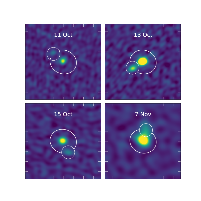
Figure 1.— ALMA observations of the Orcus-Vanth system. The images are centered on Orcus and the predicted position of Vanth is circled. Tick marks in the images are 200 mas. Vanth is clearly detected even in the lower resolution 7 Nov data.

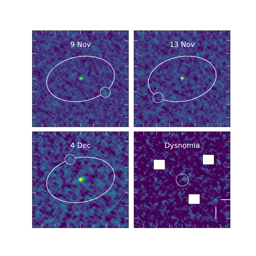
Figure 2.— ALMA observations of the Eris-Dysnomia system. The images are centered on Eris and the predicted orbit of Dysnomia is show. Predicted positions of Dysnomia based on contemporary HST observations are circled. In the bottom right panel, the three images are shifted and stacked at the position of Dysnomia, yielding a 3.5$\sigma$ detection of a source at the position of the satellite. The three positions of the shifted image of Eris are masked with white boxes. In the full frame, only one other detection as significant (marked with cross hairs in the lower right corner of the image) is seen.

3. Orcus-Vanth

A secondary source approximately 250 mas away from Orcus is clearly visible in 3 of the 4 ALMA images, and a two-gaussian fit also picks one out in the lower-resolution image from 2016 Nov 7. Using published Vanth orbital elements (Brown et al., 2010; Carry et al., 2011) we find that these detections are all along the orbital path of Vanth and consistent with the predicted position if the mean anomaly of Vanth is increased by 11 degrees, well within the current uncertainties. Flux densities measured for Orcus and Vanth are shown in Table 1.

We use the measured thermal emission to determine the sizes of Orcus and Vanth using the techniques detailed in Brown & Butler (2017, hereafter BB17). In our analysis we use a standard thermal model to calculate the thermal emission expected from a distant body. In this model, the free parameters are bolometric emmisivity, phase integral, albedo, diameter, and a beaming parameter to account for the combined effects of viewing geometry and surface thermal properties. For the emissivity and phase integral, we use typical Kuiper belt object assumptions: we constrain emissivity to be between 0.8 and 1.0, as argued in BB17, and we use the Brucker et al. (2009) empirical fit of phase integral to albedo with an allowed 50% variation from these values. Orcus and Vanth are not constrained to have any identical parameters.

We use the Markov Chain Monte Carlo scheme described in BB17 to explore the best fit parameters and their uncertainties. We fit the unresolved Orcus+Vanth Spitzer 24 and 71 $\mu$m fluxes (Stansberry et al., 2008), the unresolved Herschel 70, 100, and 350 $\mu$m flux (Fornasier et al., 2013), and the new resolved ALMA data. We assume an 850 $\mu$m emissivity of 0.685, as derived in BB17, consistent with the value also found in Lellouch et al. (2017). Figure 3 shows a collection of 30 random samples from the MCMC ensemble. The fit of the model to the data is excellent.

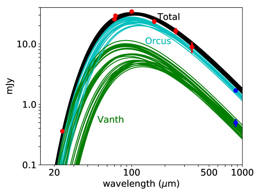
Figure 3.— A collection of 30 random samples from the MCMC ensemble compared to data from the Orcus-Vanth system. The red points are unresolved data from Spitzer and Herschel, while the blue points are the resolved data points from ALMA. The ALMA data have been scaled by the inverse of the assumed emissivity of 0.685 so that they appear at the equivalent emissivity of unity locations.

The marginalized distributions for the size and albedo of both bodies are nearly gaussian, so we report the median and 16th and 84th percentiles as our 1$\sigma$ error range. We find that Orcus has a diameter of $910^{+50}_{-40}$ km and an albedo of 0.23$\pm$0.02, while Vanth has a diameter of 475$\pm$75 km and an albedo of 0.08$\pm$0.02. Vanth is approximately half of the diameter of Orcus, with an albedo approximately 3 times smaller. These results put Vanth within the range of typical KBO albedos for objects of this size.

Without a knowledge of the density of Vanth, the mass ratio of the system is unclear. For plausible densities from 0.8 g cm^-3 (the typical density for a $\sim$500 km object) up to 1.4 g cm^-3 (the system density if Orcus and Vanth have identical densities) the mass ratio ranges between 5 and 20, while the density of Orcus ranges from 1.4$\pm$0.2 to 2.0$\pm$0.3 g cm^-3. Clearly, determining the density of Vanth is critical to understanding how the Orcus-Vanth systems fits into our understanding of large KBOs and their densities.

4. Eris-Dysnomia

No obvious detections of Dysnomia appear in the data. If we knew the predicted position of Dysnomia with respect to Eris, however, we could make a more stringent determination. The last published orbital elements of Dysnomia (Brown & Schaller, 2007) have a 30 degree phase uncertainty by the time of these observations, so are not sufficient for providing predictions. We thus use archival observations obtained using WF3 on the Hubble Space Telescope in January 2015 to update the orbital elements of Dysnomia and precisely predict its position at the time of the ALMA observations 9 months later. Astrometric offsets between Eris and Dysnomia for the times of observation are determined using the methods detailed in Brown & Schaller (2007). Table 2 shows the relative positions of Dysnomia at the times of the HST observations.

Table 2Positions of Dysnomia

JD	$\Delta$ RA	$\Delta$ Dec	observatory
	mas	mas
2457051.699	-347$\pm$2	-226$\pm$1	HST (measured)
2457054.950	string282$\pm$3	-325$\pm$2	HST (measured)
2457335.667	-383.2$\pm$1.4	-210.3$\pm$1.0	ALMA (predicted)
2457339.641	string379.5$\pm$1.5	-291.5$\pm$1.7	ALMA (predicted)
2457360.576	string159.8$\pm$1.7	string322.8$\pm$1.0	ALMA (predicted)

Table 3Orbital elements of Dysnomia

semimajor axis	string37460$\pm$80	km
inclination	string61.1$\pm$0.3	deg
period	15.78586$\pm$0.00008	days
eccentricity	string$<.004$
long. ascending node	string139.6$\pm$0.2	deg
mean anomaly	string273.2$\pm$0.02	deg
epoch (JD, defined)	string2457054.95

Note. — relative to J2000 ecliptic

We calculate the new orbit of Dysnomia using the methods described in Brown & Schaller (2007) with the updated improvements using a Markov Chain Monte Carlo scheme as described in Brown (2013). The orbit is in agreement with the previous results but with improved uncertainties. The orbit continues to be consistent with being circular, with a 1$\sigma$ upper limit to the eccentricity of 0.004, so for the final fit we constrain the orbit to be purely circular (Fig 4). Updated orbital elements are provided in Table 3.

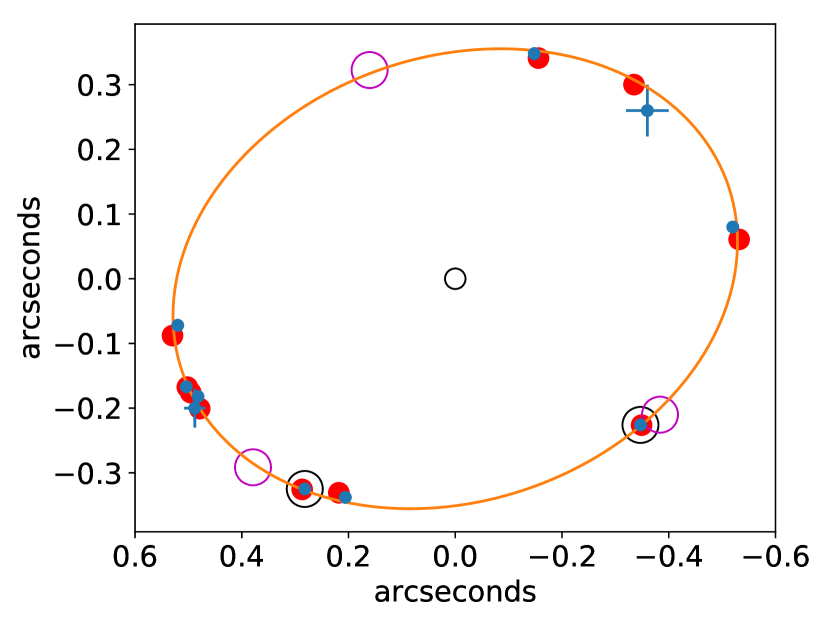
Figure 4.— A fit to the orbit of Dysnomia. Blue dots with error bars are the observations, while their best-fit locations are show as red dots. The two new data points added in this analysis are circled in blue. The large unfilled cyan circles are the predicted locations of Dysnomia at the times of the ALMA observations.

The new orbit fit allows us to predict the locations of Dysnomia at the times of the ALMA observation nine months later to within $\sim$2 mas, a fraction of the ALMA beam size. Additional astrometric uncertainty of order $\sim$10 mas ($1/4$ of the angular diameter of Eris) arises because of the potential offset between the center-of-light and center-of-mass of Eris (if, for example, Eris has a warmer pole observed obliquely). We show these predicted locations in Figures 2 and 4. A flux density enhancement occurs at the predicted location in at least 2 of the 3 observations. To increase the signal-to-noise of a potential Dysnomia detection, we shift all three images to be centered on the predicted position of Dysnomia and sum them (Figure 2). A source with a flux density of 0.13$\pm$0.03 mJy appears 16 mas from the expected position, smaller than the 30-50 mas resolution element of the data and within the range of expected astrometric uncertainties for such a low signal-to-noise source.

While we formally have a 4.2$\sigma$ detection of a potential source near the position of Dysnomia, we assess the true significance of this potential detection by performing an experiment where we shift each image by random amounts and determine the maximum flux density within 30 mas of this arbitrary position. We find values as high as the 0.13 mJy of Dysnomia only 0.02% of the time, corresponding to a 3.5$\sigma$ likelihood that the detection is indeed Dysnomia. As an additional check, we reexamine the combined image and find that in the 2.75 square arcsecond field we only see one other source as strong as the potential Dysnomia detection. Our field consists of approximately 1400 resolution elements, so we should expect to randomly detect a 3.5$\sigma$ source 33% of time, consistent with the observation. While the detection of Dysnomia is weak, we can find no reason to discount its reality. We proceed on the assumption that we have indeed detected Dysnomia.

We model the emission from Eris and Dysnomia using an identical technique as previously used for Orcus-Vanth. We assume the occultation-derived circular diameter of Eris of 2326$\pm$12 km (Sicardy, 2011) and have as the free parameters in our model fitting the beaming parameter of Eris and the diameter, albedo, and beaming parameter of Dysnomia. We again constrain the bolometric emissivity and Bond albedo as above.

We first investigate if there is any evidence for emission from Dysnomia from previous, unresolved, data. We use data at 71$\mu$m from the Spitzer Space Telescope (Stansberry et al., 2008) and data at 70, 100, and 150$\mu$m from the Herschel Space Telescope (Santos-Sanz et al., 2012). The marginalized distribution for the diameter of Dysnomia gives a 1$\sigma$ upper limit of 810 km and a corresponding 1$\sigma$ lower limit for albedo of 0.03. The unresolved data provide essentially no information on the parameters of Dysnomia. Nonetheless, if no Dysnomia is included in the fit, the flux of the shortest wavelength data is under-predicted, suggesting the possibility that a large dark body could be present in the system (Figure 5).

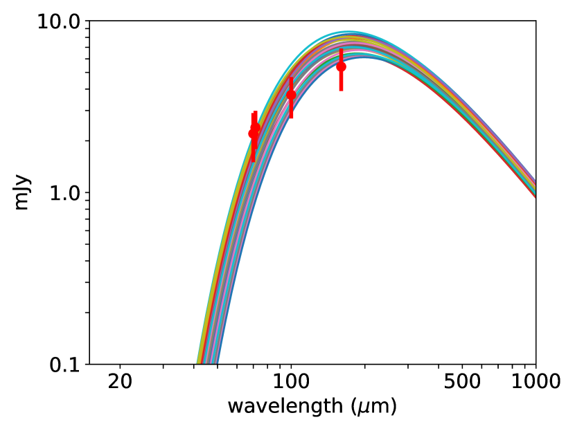
Figure 5.— A collection of 30 random samples from the MCMC ensemble compared to data from the Eris-Dysnomia system. We model only a single body and the unresolved measurements from Herschel. While the fit does not statistically support the existence of a second body in the system, it is clear that a smaller darker (thus warmer) body could improve the fit to the data.

We next fit the resolved ALMA data together with the previous unresolved data. We continue to use our earlier-derived 850 $\mu$m emissivity of 0.685 for Dysnomia, assuming it is a typical KBO. For Eris, which has a significantly different surface composition, we consider ALMA observations of Pluto (Butler et al., 2015), which suggest significantly lower brightness temperature, but it is difficult to separate the effects of emissivity and cold atmospherically buffered N₂ ice. As N₂ ice at the temperature of Eris has significantly lower volatility, we assume that ice effects are negligible and instead use the same canonical 0.685 value for emissivity. Figure 6 shows 30 samples from the MCMC ensemble to the thermal data. We find that Dysnomia has a diameter of 700$\pm$115 km with an albedo of 0.04${}^{+0.02}_{-0.01}$. Dysnomia’s size and albedo are consistent with those of typical mid-sized KBOs, but the albedo is nearly 25 times smaller than the extremely bright Eris. Allowing the density of Dysnomia to range from as low as 0.8 g cm^-3 to as high as being equal to that of Eris gives a range of system mass ratios between 37 and 115, again a large possible range.

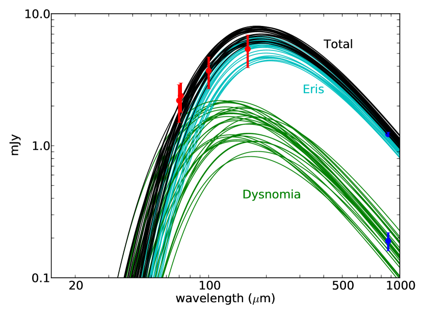
Figure 6.— A collection of 30 random samples from the MCMC ensemble compared to data from the Eris-Dysnomia system. Including the resolved ALMA data shows the presence of a mid-sized dark Dysnomia which somewhat improves the fit to the shorter wavelength data where Dysnomia’s contribution is more significant.

5. Discussion

Neither Vanth, the satellite of Orcus, nor Dysnomia, the satellite of Eris, fits the paradigm of the type of small icy collisionally derived satellite predicted by the models of Canup (2005). Such satellites form out of the icy disk surrounding the parent in the aftermath of the collision and would be expected to be nearly pure water ice like the satellites of Haumea and the small satellites of Pluto appear to be. Indeed, both Dysnomia and Vanth have the low albedos expected for typical KBOs of their size (Stansberry et al., 2008). We consider possible formation mechanisms below.

Smaller multiple-KBO systems tend to be binaries with similar-sized components (Noll et al., 2008). These are thought to either be formed through dynamical-friction-assisted capture (Goldreich et al., 2002) or to have initially formed as a pair (Nesvorný et al., 2010). Little exploration has been done of the range of possible satellite parameters that could ensue from such mechanisms, but they are generally thought to be relevant to small KBO pairs. There is no reason to expect that while mid-sized KBOs have a modest satellite fraction, the largest KBOs would preferentially have satellites owing to these same mechanisms.

Charon, the large satellite of Pluto, appears to have formed from an grazing giant impact which then left the proto-Charon largely intact, but with a low enough energy to remain bound (Canup, 2005). In simulations, collisions of undifferentiated bodies mostly yielded a satellite whose composition was unchanged from the initial impactor. The Orcus-Vanth system is plausibly explained by such a scenario. With a mass ratio between 5 and 20, Orcus-Vanth appears to be a good candidate for an analog to the Pluto-Charon system (with a mass ratio of 8), with the exception that we detect no small icy analogs of the small Pluto satellite. Brown (2008) places a brightness ratio limit of 0.1% for any more distant undiscovered objects in the Orcus system. For an icy albedo of 0.5-1.0, this limit corresponds to objects with a diameter of 15 to 20 km, smaller than at least two of the small satellites of Pluto.

The Eris-Dysnomia system is unlike any other known in the Kuiper belt. With a mass ratio between 37 and 115, Dysnomia appears intermediate between satellites such as Charon and Nyx and Hydra (with mass ratios greater than $10^{5}$; Brozović et al., 2015) Hi’iaka, the larger satellite of Haumea (with a mass ratio of $\sim$200; Ragozzine & Brown, 2009). But an albedo of $\sim$0.04 clearly shows that Dysnomia is not a reassembled product of an icy disk. We suggest two alternatives. First, it is possible that our reported detection of Dysnomia is erroneous. While we showed that the probability of a spurious detection at the predicted combined location of Dysnomia is low, robust detection at multiple locations are desired. Second, if the detection of Dysnomia is real, as the statistics suggest, our understanding of Kuiper belt satellite formation mechanisms is clearly inadequate and the range of possible satellite formation outcomes is larger than currently thought.

While large KBOs have a high fraction of satellites, a general understanding of the diverse possible formation mechanisms for these satellites is lacking. It is generally believed that giant impacts are responsible for the satellites of these KBOs, but simulations have only attempted to explain individual systems (Canup, 2005, 2011; Leinhardt et al., 2010), and no comprehensive study has explored a wide range of possible outcomes. Barr & Schwamb (2016) have suggested a general paradigm where collisions are either of the Charon-forming type or of the icy-small-fragment type, but it is not clear if this paradigm can be reconciled with the implication that Dysnomia appears not to have formed from a post-impact icy disk of material. As understanding of these satellite systems likely provides insights into populations and collisions in the early outer solar system, emphasis should be placed on both the theoretical and observational exploration of these objects.

This paper makes use of the following ALMA data: ADS/JAO.ALMA#2016.1.00830.S, ADS/JAO.ALMA#2015.1.00810.S. ALMA is a partnership of ESO (representing its member states), NSF (USA) and NINS (Japan), together with NRC (Canada), MOST and ASIAA (Taiwan), and KASI (Republic of Korea), in cooperation with the Republic of Chile. The Joint ALMA Observatory is operated by ESO, AUI/NRAO and NAOJ. The National Radio Astronomy Observatory is a facility of the National Science Foundation operated under cooperative agreement by Associated Universities, Inc. by Associated Universities, Inc.

References

- Barkume et al. (2006) Barkume, K. M., Brown, M. E., & Schaller, E. L. 2006, ApJ, 640, L87
- Barr & Schwamb (2016) Barr, A. C. & Schwamb, M. E. 2016, MNRAS, 460, 1542
- Brown (2008) Brown, M. E. 2008, in The Solar System Beyond Neptune, ed. M. A. Barucci, H. Boehnhardt, D. P. Cruikshank, & A. Morbidelli, 335–344
- Brown (2013) —. 2013, ApJ, 778, L34
- Brown & Butler (2017) Brown, M. E. & Butler, B. J. 2017, AJ, 154, 19
- Brown et al. (2010) Brown, M. E., Ragozzine, D., Stansberry, J., & Fraser, W. C. 2010, AJ, 139, 2700
- Brown & Schaller (2007) Brown, M. E. & Schaller, E. L. 2007, Science, 316, 1585
- Brown et al. (2006) Brown, M. E., van Dam, M. A., Bouchez, A. H., Le Mignant, D., Campbell, R. D., Chin, J. C. Y., Conrad, A., Hartman, S. K., Johansson, E. M., Lafon, R. E., Rabinowitz, D. L., Stomski, Jr., P. J., Summers, D. M., Trujillo, C. A., & Wizinowich, P. L. 2006, ApJ, 639, L43
- Brozović et al. (2015) Brozović, M., Showalter, M. R., Jacobson, R. A., & Buie, M. W. 2015, Icarus, 246, 317
- Brucker et al. (2009) Brucker, M. J., Grundy, W. M., Stansberry, J. A., Spencer, J. R., Sheppard, S. S., Chiang, E. I., & Buie, M. W. 2009, Icarus, 201, 284
- Butler et al. (2015) Butler, B. J., Gurwell, M., Lellouch, E., Moullet, A., Moreno, R., Bockelee-Morvan, D., Biver, N., Fouchet, T., Lis, D., Stern, A., Young, L., Young, E., Weaver, H., Boissier, J., & Stansberry, J. 2015, in AAS/Division for Planetary Sciences Meeting Abstracts, Vol. 47, AAS/Division for Planetary Sciences Meeting Abstracts, 210.04
- Canup (2005) Canup, R. M. 2005, Science, 307, 546
- Canup (2011) —. 2011, AJ, 141, 35
- Carry et al. (2011) Carry, B., Hestroffer, D., DeMeo, F. E., Thirouin, A., Berthier, J., Lacerda, P., Sicardy, B., Doressoundiram, A., Dumas, C., Farrelly, D., & Müller, T. G. 2011, A&A, 534, A115
- Cook et al. (2017) Cook, J. C., Binzel, R. P., Cruikshank, D. P., Dalle Ore, C. M., Earle, A., Ennico, K., Grundy, W. M., Howett, C., Jennings, D. J., Lunsford, A. W., Olkin, C. B., Parker, A. H., Philippe, S., Protopapa, S., Reuter, D., Schmitt, B., Stansberry, J. A., Stern, S. A., Verbiscer, A., Weaver, H. A., Young, L. A., New Horizons Composition Theme Team, & Ralph Instrument Team. 2017, in Lunar and Planetary Inst. Technical Report, Vol. 48, Lunar and Planetary Science Conference, 2478
- Cornwell & Fomalont (1999) Cornwell, T. & Fomalont, E. B. 1999, in Astronomical Society of the Pacific Conference Series, Vol. 180, Synthesis Imaging in Radio Astronomy II, ed. G. B. Taylor, C. L. Carilli, & R. A. Perley, 187–199
- Fornasier et al. (2013) Fornasier, S., Lellouch, E., Müller, T., Santos-Sanz, P., Panuzzo, P., Kiss, C., Lim, T., Mommert, M., Bockelée-Morvan, D., Vilenius, E., Stansberry, J., Tozzi, G. P., Mottola, S., Delsanti, A., Crovisier, J., Duffard, R., Henry, F., Lacerda, P., Barucci, A., & Gicquel, A. 2013, Astronomy and Astrophysics, 555, id.A15
- Fraser & Brown (2009) Fraser, W. C. & Brown, M. E. 2009, ApJ, 695, L1
- Goldreich et al. (2002) Goldreich, P., Lithwick, Y., & Sari, R. 2002, Nature, 420, 643
- Greisen (2004) Greisen, E. W. 2004, in Astronomical Society of the Pacific Conference Series, Vol. 281, Astronomical Data Analysis Software and Systems XI, ed. D. A. Bohlender, D. Durand, & T. H. Handley, 260–264
- Kiss et al. (2017) Kiss, C., Marton, G., Farkas-Takács, A., Stansberry, J., Müller, T., Vinkó, J., Balog, Z., Ortiz, J.-L., & Pál, A. 2017, ApJ, 838, L1
- Leinhardt et al. (2010) Leinhardt, Z. M., Marcus, R. A., & Stewart, S. T. 2010, ApJ, 714, 1789
- Lellouch et al. (2017) Lellouch, E., Moreno, R., Müller, T., Fornasier, S., Santos-Sanz, P., Moullet, A., Gurwell, M., Stansberry, J., Leiva, R., Sicardy, B., Butler, B., & Boissier, J. 2017, A&A, 608, A45
- Muders et al. (2014) Muders, D., Wyrowski, F., Lightfoot, J., Williams, S., Nakazato, T., Kosugi, G., Davis, L., & Kern, J. 2014, in Astronomical Data Analysis Software and Systems XXIII, ed. N. Manset & P. Forshay, 383–386
- Nesvorný et al. (2010) Nesvorný, D., Youdin, A. N., & Richardson, D. C. 2010, AJ, 140, 785
- Noll et al. (2008) Noll, K. S., Grundy, W. M., Chiang, E. I., Margot, J.-L., & Kern, S. D. 2008, in The Solar System Beyond Neptune, ed. M. A. Barucci, H. Boehnhardt, D. P. Cruikshank, & A. Morbidelli, 345–363
- Parker et al. (2016) Parker, A. H., Buie, M. W., Grundy, W. M., & Noll, K. S. 2016, ApJ, 825, L9
- Ragozzine & Brown (2009) Ragozzine, D. & Brown, M. E. 2009, AJ, 137, 4766
- Ragozzine (2009) Ragozzine, D. A. 2009, PhD thesis
- Santos-Sanz et al. (2012) Santos-Sanz, P., Lellouch, E., Fornasier, S., Kiss, C., Pal, A., Müller, T. G., Vilenius, E., Stansberry, J., Mommert, M., Delsanti, A., Mueller, M., Peixinho, N., Henry, F., Ortiz, J. L., Thirouin, A., Protopapa, S., Duffard, R., Szalai, N., Lim, T., Ejeta, C., Hartogh, P., Harris, A. W., & Rengel, M. 2012, A&A, 541, A92
- Sicardy (2011) Sicardy, B. . . o. 2011, Nature, 478, 493
- Stansberry et al. (2008) Stansberry, J., Grundy, W., Brown, M., Cruikshank, D., Spencer, J., Trilling, D., & Margot, J.-L. 2008, in The Solar System Beyond Neptune, ed. M. A. Barucci, H. Boehnhardt, D. P. Cruikshank, & A. Morbidelli, 161–179
- Thompson et al. (2001) Thompson, A. R., Moran, J. M., & Swenson, G. W. 2001, Interferometry and Synthesis in Radio Astronomy, 2nd Edition (New York, New York: Wiley-Interscience)
- Weaver et al. (2016) Weaver, H. A., Buie, M. W., Buratti, B. J., Grundy, W. M., Lauer, T. R., Olkin, C. B., Parker, A. H., Porter, S. B., Showalter, M. R., Spencer, J. R., Stern, S. A., Verbiscer, A. J., McKinnon, W. B., Moore, J. M., Robbins, S. J., Schenk, P., Singer, K. N., Barnouin, O. S., Cheng, A. F., Ernst, C. M., Lisse, C. M., Jennings, D. E., Lunsford, A. W., Reuter, D. C., Hamilton, D. P., Kaufmann, D. E., Ennico, K., Young, L. A., Beyer, R. A., Binzel, R. P., Bray, V. J., Chaikin, A. L., Cook, J. C., Cruikshank, D. P., Dalle Ore, C. M., Earle, A. M., Gladstone, G. R., Howett, C. J. A., Linscott, I. R., Nimmo, F., Parker, J. W., Philippe, S., Protopapa, S., Reitsema, H. J., Schmitt, B., Stryk, T., Summers, M. E., Tsang, C. C. C., Throop, H. H. B., White, O. L., & Zangari, A. M. 2016, Science, 351, aae0030