A Java Application to Characterize Biomolecules and Nanomaterials in Electrolyte Aqueous Solutions

Abstract

The electrostatic, entropic and surface interactions between a macroion (nanoparticle or biomolecule), surrounding ions and water molecules play a fundamental role in the behavior and function of colloidal systems. However, the molecular mechanisms governing these phenomena are still poorly understood. One of the major limitations in procuring this understanding is the lack of appropriate computational tools. Additionally, only experts in the field with an extensive background in programming, who are trained in statistical mechanics, and have access to supercomputers are able to study these systems. To overcome these limitations, in this article, we present a free, multi-platform, portable Java software, which provides experts and non-experts in the field an easy and efficient way to obtain an accurate molecular characterization of electrical and structural properties of aqueous electrolyte mixture solutions around both cylindrical- and spherical-like macroions under multiple conditions. The Java software does not require outstanding skills, and comes with detailed user-guide documentation. The application is based on the so-called Classical Density Functional Theory Solver (CSDFTS), which was successfully applied to a variety of rod-like biopolymers, rigid-like globular proteins, nanoparticles, and nano-rods. CSDFTS implements several electrolyte and macroion models, uses different level of approximation and takes advantage of high performance Fortran90 routines and optimized libraries. These features enable the software to run on single processor computers at low-to-moderate computational cost depending on the computer performance, the grid resolution, and the characterization of the macroion and the electrolyte solution, among other factors. As a unique feature, the software comes with a graphical user interface (GUI) that allows users to take advantage of the visually guided setup of the required input data to properly characterize the system and configure the solver. Several examples on nanomaterials and biomolecules are provided to illustrate the use of the GUI and the solver performance.

Program Summary:

Program Title: CSDFTS

Journal Reference:

Catalogue identifier:

Program obtainable from: CPC Program Library; The University at Texas at San Antonio, TX, USA.

Licensing provisions: UTSA license.

Distribution format: zip

Programming language: Java 1.8.

Computer: any computer at least with 2.8 GHz speed.

Operating system: Windows, Linux (Ubuntu, Fedora, Centos, Debian), and Mac OSX.

RAM: It is required at least 6 GBs. We Recommend 12 GBs for highly demanding calculations.

Classification: 3, 10.

External routines/libraries: GNU gawk installation is required if the user wants to calculate the protein volume using the 3v application.

Subprograms used: Jmol, pdb2pqr, Propka, Provol, 3v.

Nature of problem: A rich and complex, yet not fully understood, electrical double layer (EDL) formation arises when a nanoparticle or biomolecule is immersed in a liquid solution.

Solution method: The Java application is based on the Classical Density Functional Theory Solver (CSDFTS).

Unusual features: The software incorporates a graphical user interface which eliminates the arduous and error-prone manual entry of data, and substantially reduces the time spent on the setup of the information required to characterize the macroion and the electrolyte solution. Additionally, each GUI screen provides helpful information about how to fill out the input data by simply holding the mouse pointer over the corresponding text or blank box. the GUI tests all the input data before running the CSDFTS to avoid the incorrect use of the software and prevent meaningless results.

Additional comments: the GUI requires a variety of the user’s computer applications, which are a part of the basic operating systems. The GUI uses “Activity Monitor”, “procexp.exe”, and “gnome-system-monitor” (or “top”) applications for Mac, Windows and Linux users, respectively, to monitor the user’s computer performance. It also uses “Terminal.app”, “cmd.exe” and “gnome-terminal” (or “xterm”) for Mac, Windows, and Linux users, respectively, to display the CSDFT calculations.

Running time: the software to run on single processor computers at low-to-moderate computational cost depending on the computer performance, the grid resolution, and the characterization of the macroion and the electrolyte solution.

I Introduction

A rich and complex, yet not fully understood, electrical double layer (EDL) formation arises when a nanoparticle or biomolecule is immersed in a liquid solution key-1 ; key-9 ; key-2 . In such conditions, the structural and thermodynamic properties of the liquid surrounding the macroion are shown to be very different from those corresponding to the bulk phase, which in turn, have a high impact on the behaviors and functions of the macroion. For instance, physicochemical properties of nanomaterials such as particle size (PS), shape, Zeta potential (ZP), and surface charge density (SCD) have significant effects on their stability, circulation in blood and absorption into cell membranes key-3 ; key-4 ; key-5 ; key-6 . Alteration of the pH and electrolyte conditions modify the SCD and ZP, which affect the binding of nanomaterials to biological tissue and target them to specific sites inside the cell. Whereas, in biophysics key-7 ; key-8 ; key-10 , the formation of high order structures, including bundles and networks, involve interactions between highly charged linker proteins and biopolymers that are often modulated by the biological environment. The environment has been shown to have a profound impact on biological functions. For instance, ZP and SCD in microfilaments, nucleic acids, and globular proteins play a fundamental role in the stabilization of these systems due to charge residue groups on their surface. Extremely positive or negative ZP values cause larger repulsive forces. This repulsion between macroions with similar electric charge prevents aggregation of the macroions and thus ensures easy redispersion. Adversely, altering the ZP to the point at which it exhibits zero net charge may decrease stabilization forces and promote agglomeration.

Beyond the substantial progress done in the characterization of these colloidal systems, the complex interplay between the physicochemical properties of macroions and biological environment still remains elusive due to the lack of appropriate methodologies. Conventional computational tools and approaches are limited by their approximations and computational cost. Certainly, the current understanding of EDL properties of macroions is based mainly on mean-field theories like the non linear Poisson-Boltzmann (NLPB) formalism and its modifications key-10 , which consider electrostatic potential interactions only. Furthermore, the poor resolution and sensitivity of current experimental techniques limit our ability to obtain information on the molecular mechanisms governing these phenomena. Thus, they may be inappropriate to explore a large number of colloidal systems. Additionally, scientific software developed to characterize solvation and electrical double layers of nanomaterials and biomolecules might be helpful in understanding these phenomena. However, they usually require specialized training and expertise in computational biology, expensive commercial licenses, and access to clusters or supercomputers, which are often an obstacle for many researchers, experimentalists, even students lacking these requirements. Thus, it is essential to develop not only more accurate and efficient approaches, but also readily accessible, friendly implementation of a software package that provides experts and non-experts a visualized guide (graphical user interface) to perform these calculations without limitations key-11 .

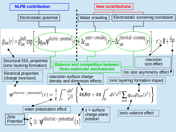
Figure 1: CSDFT theory

In this article, we present a free, multi-platform and portable Java software which provides both experts and non-experts in the field an easy and efficient way to get an accurate molecular characterization of the EDL properties for biomolecules and nanomaterials at infinite dilution. The application is based on the so-called Classical Solvation Density Function Theory (CSDFT) and its modifications, which have been shown to be particularly useful in studying multiple environmental scenarios for a variety of rod-likekey-12 ; key-13 and sphericalkey-14 ; key-15 ; key-16 rigid-like macroions without computational restriction. CSDFT extends the capabilities of NLPB formalism, eliminating the extremely high computational demands of full atomistic simulation calculations without losing important structural features of complex EDL properties (see Figure 1). It considers not only the electric, but also the entropic and many-body interactions. This feature has been particularly useful for identifying and characterizing dominant interactions and molecular mechanisms governing the behavior and function of macroions under a variety of electrolyte conditions.

In the next sections, we explain how to install, run and use the software. We also include examples to illustrate the solver performance and applicability. In Appendix A, we provide a brief summary of the approach and computational scheme implemented by the software to solve the CSDFT numerically.

II Overview

The software allows the user to use a variety of models and approaches. It provides four macroion models: nanoparticle, nanorod, globular protein, and rod-like biopolymer. For each of these models, there are two approaches to characterize the macroion size and the surface charge density: experimental and protonation/deprotonation models for nanomaterials applications, and experimental and molecular structure models for biophysics applications. Additionally, the software comes with two electrolyte approaches: NLPB and CSDFT. These approaches include 3 ion size types (Crystal, Effective and Hydrated), and two solvent models (implicit and explicit). As a unique feature, the Java application comes with a graphical user interface (GUI) which eliminates the arduous and error-prone manual entry of data, and substantially reduces the time spent on the setup of the information required to characterize the macroion and the electrolyte solution. Additionally, each GUI screen provides helpful information about how to fill out the input data by simply holding the mouse pointer over the corresponding text or blank box. The GUI also provides default values for key input parameters and preselects some relevant algorithms to speed up the setup of the input data. However, they may be easily changed at any time. Moreover, the GUI tests all the input data before running the CSDFTS to avoid the incorrect use of the software and prevent meaningless results. At the end of the calculations, the GUI generates two-dimension plots of the selected output files to provide graphical representations of the structural and electrostatic properties of the macroion EDL. Finally, all the output data files are properly saved and organized in the designated folder for post-analysis purposes.

III General considerations

III.0.1 System Requirements

The software requires at least 500 MB of disk space to install. Additional disc space is required to save the output files generated by each simulation, which may be as large as 1Gb or more. The available RAM memory required to run the software depends on many factors. Based on the examples presented in this article, most simulations require only a few Gbs whereas highly demanding calculations may demand up to 12 Gbs.

The software is portable, e.g. it does not require external libraries, leave its files or settings on the host computer, or modify the existing system and its configuration. The software comes with Java 1.8 which is configured by the installer to run the GUI. The Fortran90 codes are distributed as binary files. For biophysics applications, the software requires the molecular structure visualization java tool “Jmol” (http://jmol.sourceforge.net/) key-17 and either the java based protein volume “provol” (gmlab.bio.rpi.edu/) key-26 or the Unix based “v3” (http://3vee.molmovdb.org/volumeCalc.php) key-18 applications. These open sources are compiled and distributed along with the software. To use the latter application, the user’s computer needs to have the GNU “gawk” application installed (https://www.gnu.org/software /gawk/). The software also includes “pdb2pqr” and “propka” binary files with the necessary libraries to perform molecular structure calculations (http://apbs-pdb2pqr.readthedocs.io /en/latest/pdb2pqr/index.html) key-19 . Additionally, the GUI requires a variety of the user’s computer applications, which are a part of the basic operating systems. In particular, the GUI uses “Activity Monitor”, “procexp.exe”, and “gnome-system-monitor” (or “top”) applications for Mac, Windows and Linux users, respectively, to monitor the user’s computer performance. It also uses “Terminal.app”, “cmd.exe” and “gnome-terminal” (or “xterm”) for Mac, Windows, and Linux users, respectively, to display CSDFT calculations.

III.0.2 Installation

The software is distributed as a single zip file containing the self-installer application. The user does not need “Root” or “Admin” permissions to install the software on the user’s home directory. The user may unzip the file on the desktop directory, open the resulting folder, then double-click the self-installer application to run the wizard setup and follow a number of module steps (See Figure 2). The installer creates the folder “CSDFTS” in the chosen directory to save the software source files, including the GUI executable “CSDFTS-software”. If selected, the installer also creates an icon on the desktop for easy access to run the GUI. The software was successfully installed and tested on a variety of operating systems (Windows 7 and 10, Sierra, Centos 7, Ubuntu 14, Fedora 24, Debian 8) and provides an uninstaller application for easy removal.

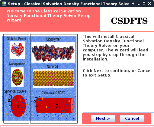
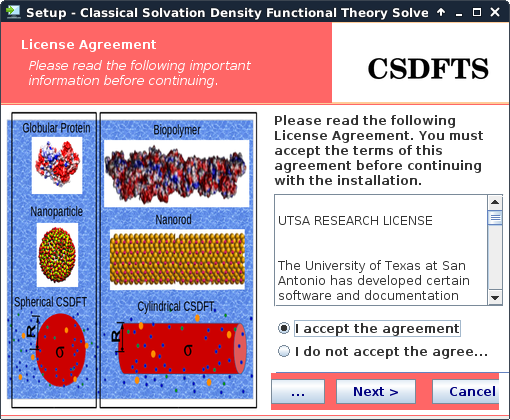
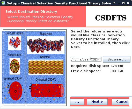
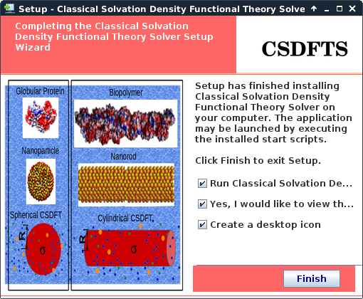
Figure 2: Multi-platform JAVA self-installer application

III.0.3 Output files

During the first simulation the GUI creates a folder named “CSDFTS_Workspace” in “My Documents” and “$HOME” directory for Windows and Unix operating systems, respectively. Within this folder, the GUI creates one sub-folder per each simulation to save and organize all the corresponding output data files. The name of the sub-folders follows the convention:

Analysis_<<macroion-electrolyte>>_<<Date>>__<<Time>>, where <<macroion- electrolyte>> is the macroion and electrolyte model selected by the user, <<Date>> is the current date, and <<Time>> is the real time when the model was selected (see Figure 3).

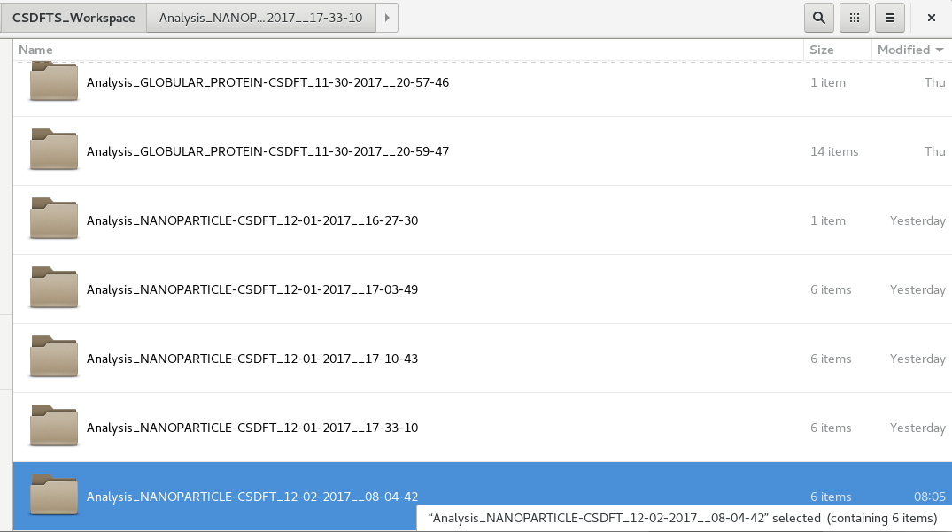
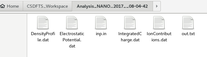
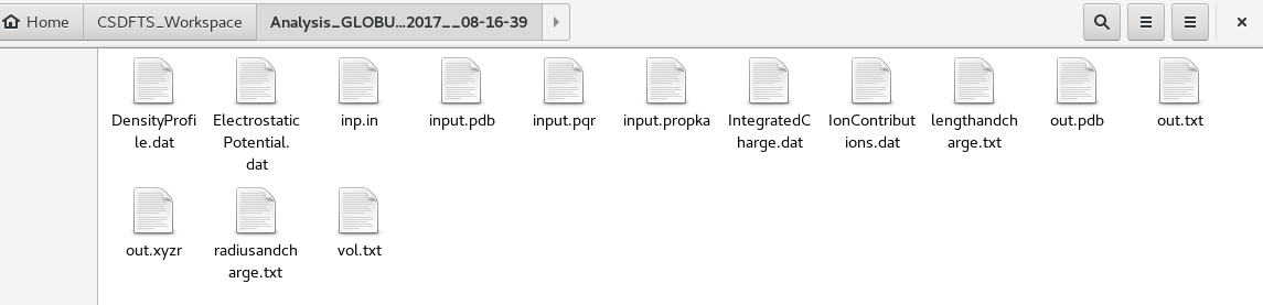
Figure 3: CSDFTS Workspace.

The GUI generates the following output files: “DensityProfile.dat (normalized ions and water density profile distributions”); “ElectrostaticPotential.dat” (mean electrostatic potential); “IntegrateCharge.dat” (the integrated charge), and “IonContributions.dat”(normalized electrostatic potential energy, particle crowding entropy energy, and ion-ion electrostatic correlation energy to the ionic potential of mean force). Explicit expressions for these properties are provided in Appendix A. The size of these files may vary depending on the number of ions species, number of grid points, and electrolyte model. These files are formatted in a multi-column arrangement where the row number corresponds to the number of grid points, the first column contains the discretized distance in unit of Å and the remaining column(s) provide the numerical solution(s) (see Table 1). Other relevant data including SCD, ZP, and PS are saved in the log file “out.txt”, whereas information on the input data and solver configuration are included in the files “inp.in” and “input.file” for spherical and cylindrical macroions, respectively. If the molecular structure option is selected for biophysical applications, the GUI generates the following additional files: “input.pdb” (copy of the molecular structure uploaded by the user); “input.pqr” (pdb2pqr output data); “input.propka” (propka output data) ; “out.pdb” (molecular structure information with heterogem atoms removed); “out.xyzr” (atomic positions in xyzr format); “vol.txt” (3v and provol output data including information on the macroion surface and volume as well as the number of residues and atoms); “lengthandcharge.txt” (total macroion charge and dimensions), and “radiusandcharge.txt” (parameters characterizing the macroion radius and charge density).

File name	Units	Description
DensityProfile.dat		$\begin{array}[]{c}\textrm{The first column is for distances. The second column corresponds to}\\ \textrm{the first ion species selected in ion model section, and so on. }\\ \textrm{If the CSDFT is selected, the last column corresponds to water}\end{array}$
ElectrostaticPotential.dat	KT/e	$\begin{array}[]{c}\textrm{The first column is for distances.}\\ \textrm{the second column contains the values of the mean }\end{array}$
IntegratedCharge.dat	e	$\begin{array}[]{c}\textrm{The first column is for distances. }\\ \textrm{the second column contains the values of the integrated charge}\end{array}$
IonConstributions.dat	J/KT	$\begin{array}[]{c}\textrm{The first column is for distances. Then, there is one set of columns per}\\ \textrm{contribution. The number of columns per contribution is equal to the}\\ \textrm{number of ion species. The order of the set of columns }\\ \textrm{from left to right reads : the electrostatic potential }\\ \textrm{energy, excluded volume energy, the ion-ion correlation energy, }\\ \textrm{and the potential of mean force (sum of the previous contributions). }\\ \textrm{The order of the columns in each set of contributions is the following:}\\ \textrm{first column corresponds to the first selected ion species, and so on.}\end{array}$

Table 1: Output Files created by CSDFTS.

IV Graphical User Interface: Use and Applications

IV.1 GUI Description

In this section we describe the screen sequence generated by the GUI. The first, second and third screens correspond to “project window”, ”model window”, and “results visualization window”, respectively. Each screen provides information to help the user fill out the input data by moving the mouse pointer over the corresponding text or blank box (see Figure 4).

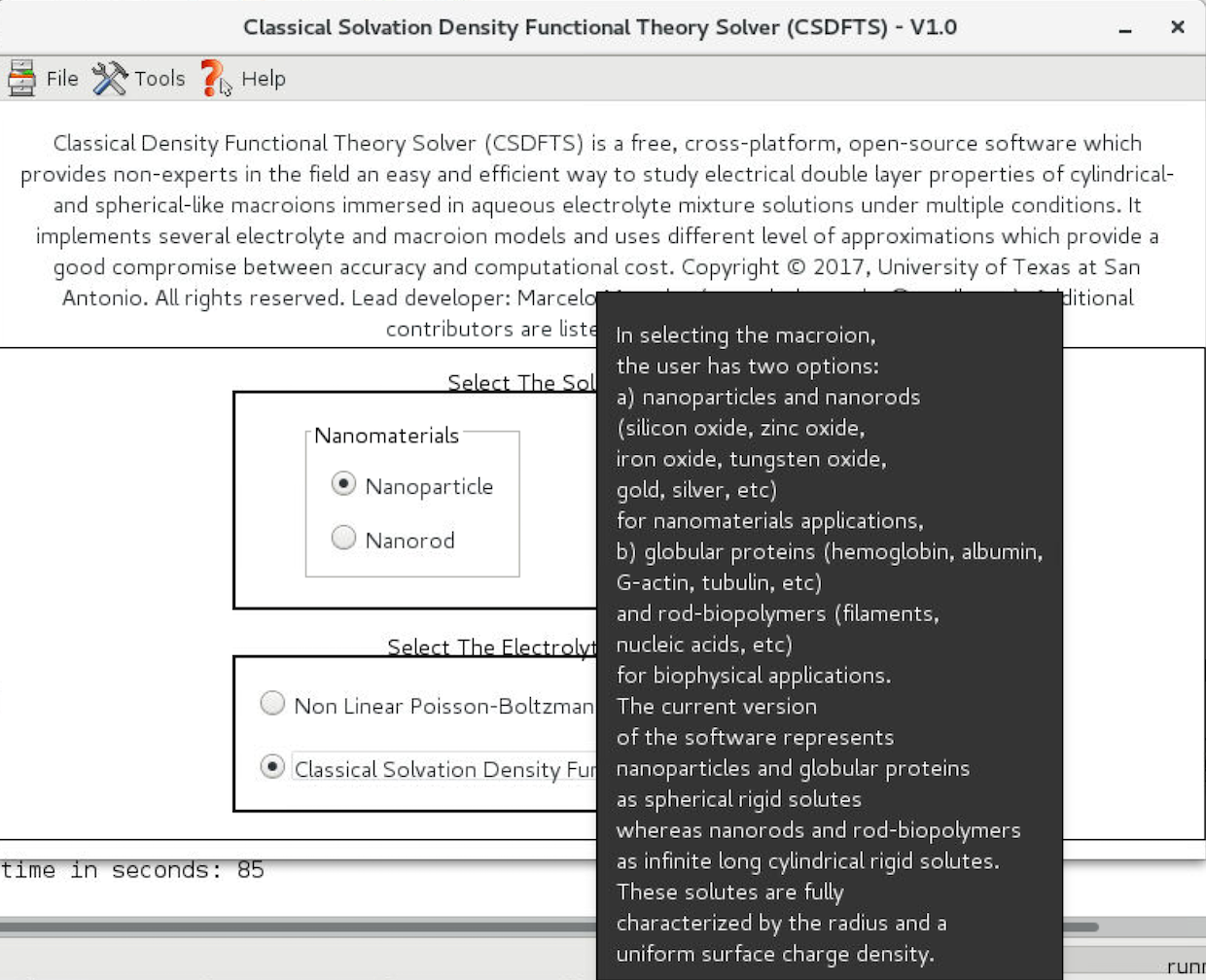
Figure 4: Help Messages.

IV.1.1 Project Window: Selection of the solute geometry model and electrolyte solution theory

The Project window shown in Figure 5 is the main screen which provides user access to the Menu, Information and Model Sections.

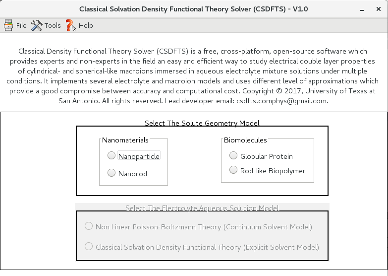
Figure 5: Project Window - main screen.

The menu section, located at the top left corner of the window, contains the File, Tools and Help menus. The File Menu contains the Results Visualization and Exit options (see Figure 6(a)). The Results Visualization option may be used after running the simulation. This option allows users to select output file(s) and visualize the solution(s) in two dimensional plot(s).

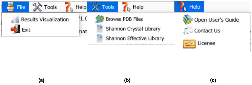
Figure 6: (a) File Menu. (b) Tools Menu. (c) Help Menu.

The Tools Menu contains the Browse PDB files, Crystal Ion Library, Effective Ion Library and Hydrated Ion Library options (see Figure 6(b)). The tool Browse PDB files is used for biophysical applications only. It allows users to open a web browser and download protein molecular structure(s) from the protein data base web page (http://www.rcsb.org/). The user may use this tool at anytime. The Ion Library tools provide the user access to the tables pretabulated with specific information on ion species, valences and diameters that are required to characterize the electrolyte aqueous solution. These tools can be used to redefine existing ion species and define new ion species as well. The last menu in Figure 6(c) is the Help Menu which provides access to the user’s guide, software license and contact information.

The Solute Geometry Model section is located at the central-bottom part of the window. To select the macroion (solute), the user has four options: Nanoparticles and nanorods for nanomaterials applications, or globular proteins and rod-biopolymers for biophysical applications.

The Electrolyte Aqueous Solution Model is located right below the Solute geometry model. CSDFTS offers two electrolyte aqueous solution theories. NLPB uses an implicit solvent model and considers electric interactions only, whereas, CSDFT uses an explicit solvent model (SPM) and considers not only the electric, but also the entropic and ion-ion correlation interactions. More information on solvent and ion models is provided in Appendix A. The selection of the EDL model mainly depends on the computational resources, the electrolyte conditions, physicochemical properties of the solute, and the accuracy required for the numerical solution (illustrative examples are provided below). As a rule of thumb, NLPB is more efficient, but less accurate than CSDFT. It is worth mentioning that CSDFT is a unique feature of the software, whereas NLPB theory is included for testing and comparison purposes, mostly. Indeed, there are other efficient programs based on implicit solvent models such as APBS key-20 and MPBEC key-21 who provide the solution for both symmetric and asymmetric macroion shapes.

IV.1.2 Model Window: system and solver configuration

Once the Solute Geometry Model and the Electrolyte Aqueous Solution Model are selected in the project window, the GUI automatically opens a second screen, the model window. In this screen, most of the text based user interaction occurs (see Figure 7). It contains the following modules: Electrolyte Model, Solute Model, and Numerical Scheme and Runtime Options.

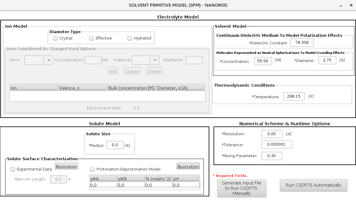
(a) Nanomaterials screen

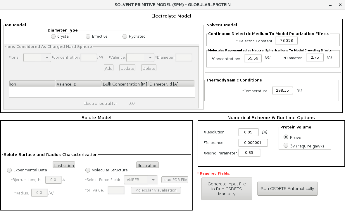
(b) Biophysics screen

Figure 7: Model window option

The Ion Model section shown in Figure 8 allows users to characterize the electrolyte solution by providing the bulk concentration $[\rho_{i}^{0}]$ and the valence $z_{i}$ for each ion species $i$. In NLPB theory, ions are represented as point-like particles, and consequently, there is no need to define the ion sizes. Whereas, in CSDFT each ionic species $i$ is represented by charged hard spheres of diameter $d_{i}$. In this case, CSDFTS offers a pretabulated crystal, effective and hydrated ionic diameter types, which are estimated using different experimental techniques key-22 . To characterize the electrolyte solution, the user has to select the first ion species and its properties, then click the button “Add”, and subsequently repeat the procedure to add more ion species. The “Delete” and “Update” buttons allow users to remove and change the properties of a previously selected ion. Once the user selects all the ion species (e.g. valence and bulk concentration), the electroneutrality condition (e.g. $\sum_{i}z_{i}[\rho_{i}^{0}]=0$) must be satisfied. The status of this condition is displayed at the bottom of this section. Note that only ion species comprising the electrolyte solution must be defined in this section. Hydrogen and Hydroxide ions controlling the pH level of the electrolyte solution are assigned by CSDFTS automatically.

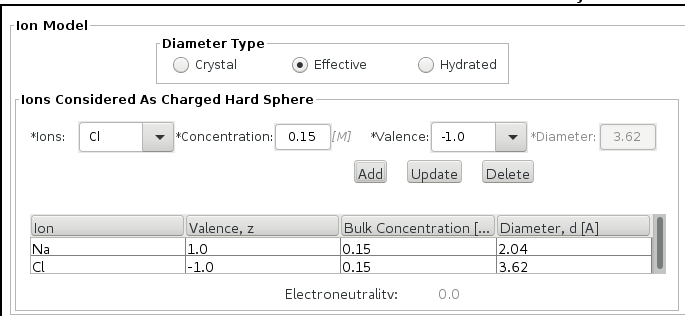
Figure 8: Ion Model.

The Solvent Model section shown in Figure 9 allows users to characterize the structural and electric properties of the solvent. Both NLPB and CSDFT consider the solvent as neutral polar molecules. NLPB only requires the value of the uniform bulk dielectric permittivity constant $\epsilon$ to model the solvent electrical properties. CSDFT additionally requires the solvent molar bulk concentration $[\rho_{w}^{0}]$ and molecular diameter $d_{w}$ to model the solvent entropy properties. The default values displayed in this section correspond to the experimental values for water. More details on solvent models are provided in Appendix A.

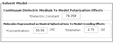
Figure 9: Solvent Model.

Regarding the Solute Model section, Figure 10 a) corresponds to nanomaterials, whereas Figure 10 b) corresponds to biomolecules. The current version of the software represents nanoparticles and globular proteins as spherical rigid solutes. Nanorods and rod-biopolymers are represented as infinitely long cylindrical rigid solutes. These solutes are characterized by the effective radius, as well as, the surface charge density $\sigma$ and the Bjerrum length $\ell$ for spherical and cylindrical shapes, respectively.

For nanomaterials it is required to provide the effective radius which is usually obtained from experiments. For biomolecules there are two ways to characterize the solute size. The user may either provide this information from experiments (Experimental data model) or it can be estimated from the molecular structure (Molecular structure model).

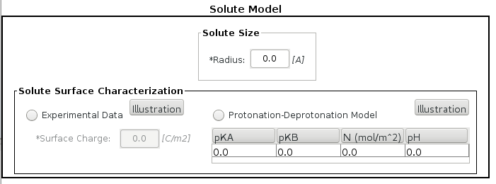
(a) Nanomaterials

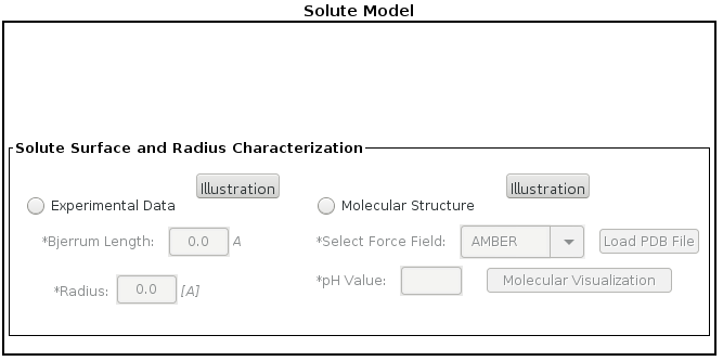
(b) Biomolecules

Figure 10: Solute Model.

A novel feature of the software is the option to calculate the macroion surface charge density $\sigma$ arising from the protonation/deprotonation reactions of the dissociable functional groups at the solid/liquid interface. The user can also click the Illustration buttons to visualize the different options and models (see Figure 11). For nanomaterials, this charging / discharging mechanism has traditionally been described using surface complexation models (SCMs), where titration of surface groups is described by the pH level and an ensemble of mass balance equilibria with associated equilibrium constants (see Appendix A). This approach is included in the protonation/deprotonation model where the user has to provide the equilibrium constants pKa and pKb for protonation and deprotonation of the active functional group, respectively, as well as the number density of total functional groups on the surface N, and the pH level (see Figures 10 a)). The resulting SCD depends on the ZP and vise-versa. A different scenario is presented for globular proteins and rod-biopolymers since the titration is usually described by a set of empirical rules relating the protein structure to the equilibrium constant values of ionizable groups (residues). This mechanism is included in the Molecular structure model option where the user has to upload the molecular structure (pdb file), select a force field, and define the pH level as shown in Figure 10 b). This uncharged molecular structure in pdb format is used by the software to automatically run the pdb2pqr / propka application (http://sourceforge.net/projects/pdb2pqr/). This application assigns atomic charges and sizes, adds missing hydrogens, optimizes the hydrogen bonding network, and renormalizes atomic charges of the residues exposed to the surface due to pH effects (protonation/deprotonation process). Afterwards, the GUI uses the molecular structure in pdb format to automatically run either the provol (default) or 3v application to estimate the total macroion volume by rolling a probe particle of radius 1.4Å and using a grid mesh of 0.5Å. Finally, the GUI uses the information obtained from the total protein charge and volume to estimate the effective solute radius as well as the uniform surface charge density and Bjerrum length for spherical and cylindrical shapes, respectively. For each of these approaches, the GUI opens an external terminal window to display these calculations (see Figure 12). It also opens a RAM memory window to monitor the user’s computer performance (see Figure 13). The GUI closes these windows once the calculations are over and enables the execution buttons “Generate the input file and run CSDFT manually” and “run CSDFT automatically” to run CSDFT.

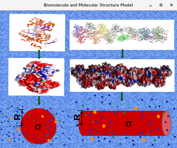
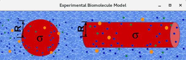
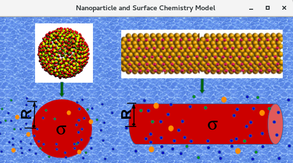
Figure 11: Illustrations

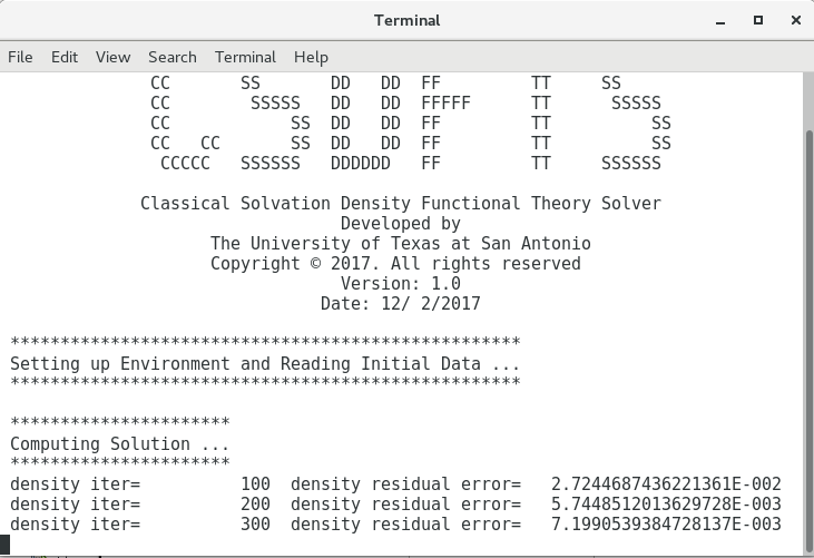
Figure 12: CSDFTS calculations

Another important feature for biophysics applications is the molecular visualization tool. After all the aforementioned calculations are over, the user can visualize the uploaded molecular structure which provides a detailed molecular characterization including the amino acid sequence and the number and type of residues exposed to the electrolyte (see Figure 14). Alternatively, the user may select the experimental data option to provide the values of these parameters from experiments. In this case, there is no waiting time to run CSDFTS.

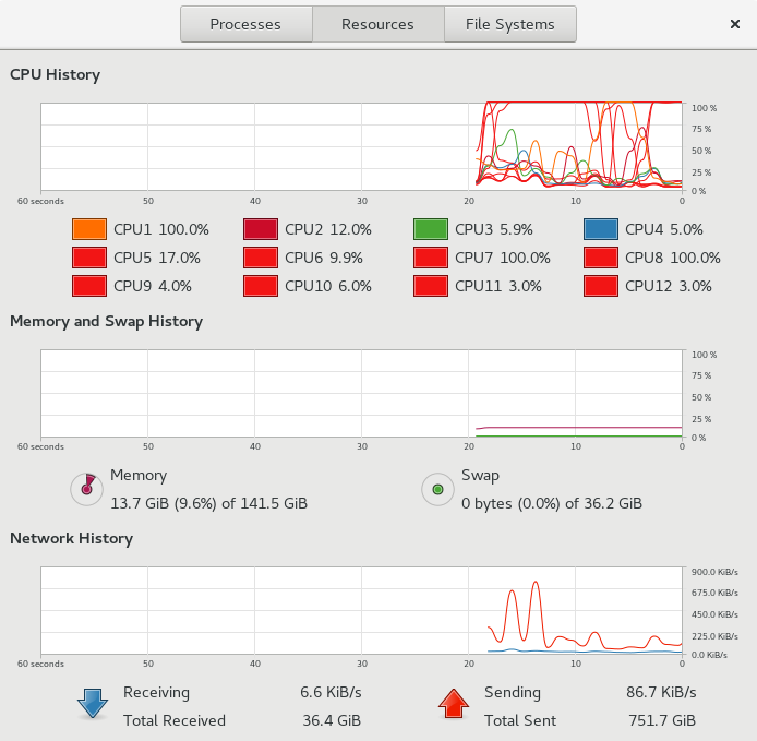
Figure 13: User’s computer performance on Linux operating systems

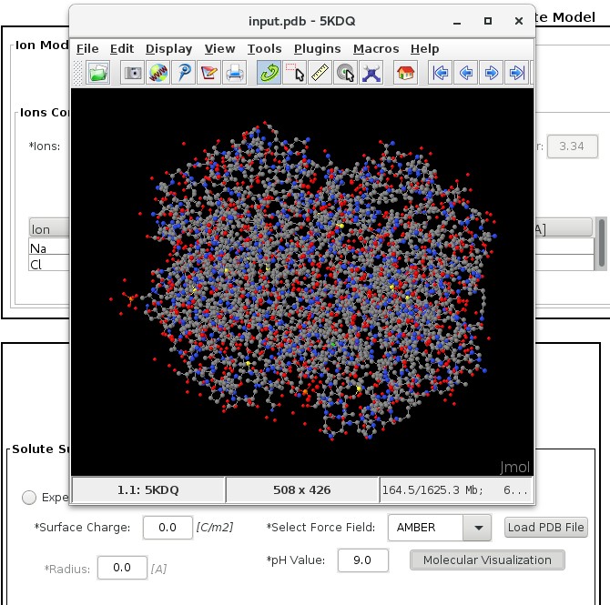
Figure 14: Molecular structure visualization.

The Thermodynamic Conditions option is used to define the electrolyte solution temperature. The default value displayed in Figure 15 corresponds to the room temperature.

Figure 15: Electrolyte solution temperature.

The Numerical Scheme and Runtime Option section shown in Figure 17 allows the user to configure key parameters that play a fundamental role in the solver performance. They control the accuracy and computational cost. The tolerance number represents the numerical error required by the user to numerically obtain the normalized density profile solutions. A minimum of six digits of precision is highly recommended (default value). The radial grid resolution represents the regular separation distance h between two consecutive points in the domain discretized of the radial distance to solve CSDFT numerically. The value recommended for this parameter is 0.05Å which has been shown to work for most applications on computers without RAM memory restrictions. The domain of the solution ranges from the macroion surface (e.g. the radius R) to the cutoff L. The latter is determined automatically by CSDFTS to provide the correct (long range) asymptotic behavior of the mean electrostatic potential, and consequently, satisfy the electroneutrality condition of the system. The number of grid points is calculated as follows $N=(L-R)/h+1$. The Mixing Parameter is a number between 0 and 1 which helps the solver to reach stability and convergence in the solution iteratively. The default value for this parameter is 0.35. It is required for the protonation/deprotonation model only.

We note that the high resolution and tolerance generate high computational cost, allocated RAM memory, solver stability and accuracy, but slow the rate of convergence on the calculations. The user may use lower resolution to speed up the calculations and reduce the allocated RAM memory at the risk of loosing convergence in the CSDFTS iterations. In that case, the solver will stop the simulation after 10000 iterations. The user may also kill the process using standard approaches (e.g. “Ctrl+c”, etc). More details on the numerical solver scheme are provided in Appendix A.

After all changes on preselected parameters and options are completed, all boxes are filled out and precalculations are over, the user may either press the button Generate the input file and run CSDFT manually or run CSDFT automatically. The GUI tests all the input data, and sends the user warning messages if unusual/nonphysical values are assigned to the required parameters or missing information is detected (see Figure 16).

Figure 16: Warning messages.

We highly recommend the user to use the option run CSDFT automatically. The other option is mainly for those users that have computer skills and prefer to run the simulations using command line. In this case, the GUI generates the input file “inp.in” for spherical solutes and “inputfile.in” for cylindrical solutes. To run CSDFTS manually in Linux operating systems, for instance, the user should open a terminal, change the current directory to the corresponding output sub-folder directory and type “~/CSDFT/Linux/sphere_linux.sh inp.in” for spherical solutes or “~/CSDFT/Linux/cylinder_linux.sh inputfile.in” for cylindrical solutes. A similar procedure should be performed for other operating systems.

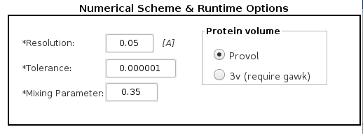
Figure 17: Numerical scheme and runtime options.

IV.1.3 Results Visualization

If the “run CSDFT automatically” option is selected, the results visualization window appears once the simulation is over. This screen allows the user to select the output file(s) and visualize the numerical solution(s) as a function of the radial separation distance in two dimension plot(s) (see Figures 18). To change the plot properties the user must right click on the desired plot (see Figure 18 c)). The user can also visualize the data on spreadsheets as shown in Figure 18 b).

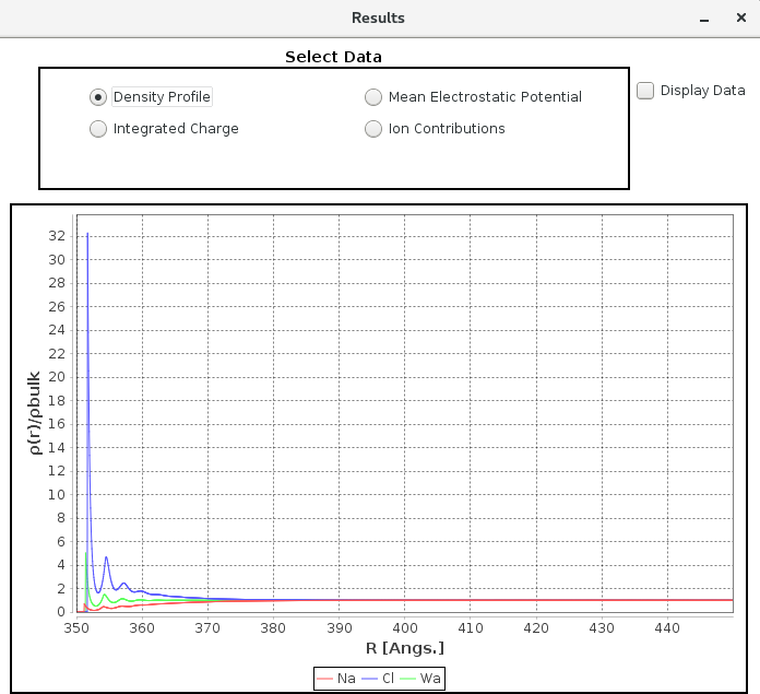
a)b)

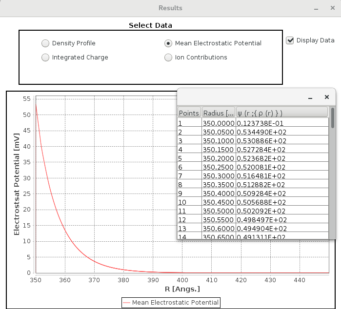
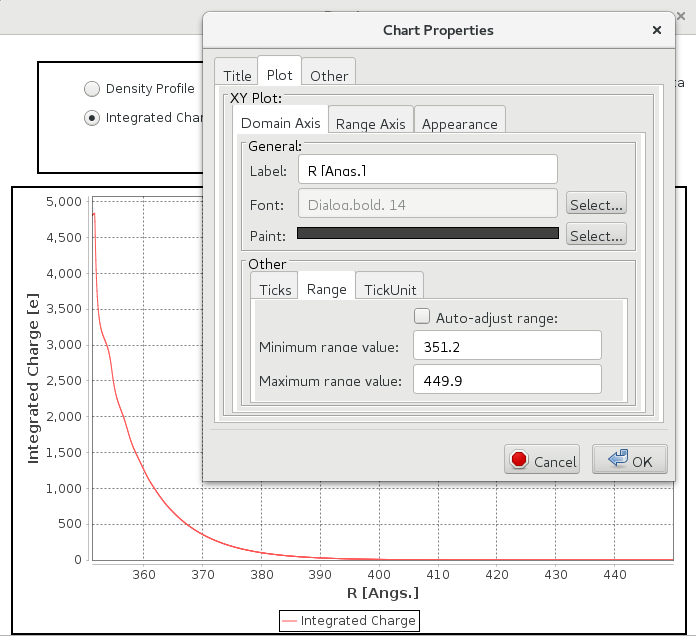
c)d)

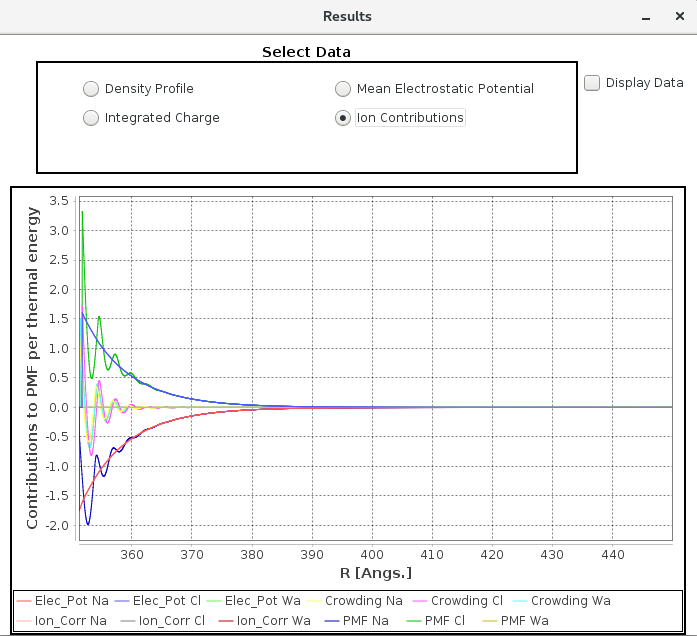
Figure 18: Results Visualization

IV.2 Quick start

The user is recommended to follows these simple steps:

• On the first screen, select the macroion type and subsequently the electrolyte model.

• On the second screen, select the ions and provide the corresponding concentrations. Make sure to fulfill the electroneutrality condition. Next, define the solvent model. The dielectric permittivity value may be changed if needed. If CSDFT was selected, the solvent concentration and molecule size may be also changed. Subsequently, configure the solver. The resolution and tolerance may be changed depending on the user’s computer performance and available RAM memory. The default values may be used if there is no RAM memory restrictions. Otherwise, decrease the resolution accordingly. For nanomaterials applications and protonation / deprotonation models, the mixing parameter may be changed if needed. For biophysics applications and the molecular structure option, the protein volume application may be changed depending on the user’s operating system. The default application works for all the operating systems whereas “3v” only works for Unix operating systems and requires the GNU gawk application installed on the user’s computer. As a rule of thumb, the latter runs faster and requires less allocated RAM memory. Next, the temperature may be changed if needed. The last step is the selection of the solute model. For nanomaterials applications, select either the experimental or protonation / deprotonation option and provide the corresponding information. Now the software is ready to run the CSDFTS. For biophysics applications, select either the experimental or the molecular structure option and provide the corresponding information. In the latter case, select the force field and set up the pH before uploading the molecular structure. Wait until some calculations on the molecular structure are over. Afterwards, the molecular structure my be visualized. Finally, select either the “Generate the input file and run CSDFT manually” or “run CSDFT automatically”.

• If the “run CSDFT automatically” was selected, an additional screen is available to visualize solutions in 2D plots.

• If there is any issue in the previous steps, close all screens and start over again. Double check that all the input data and selected options are appropriate for the required simulation and change those parameters to improve the CSDFTS convergence and the user’s computer performance.

IV.3 Examples

In this section we analyze several macroions under different electrolyte conditions (see Table 2). We ran these simulations on several operating systems and CPU processors. The results shown in the present article corresponds to those obtained on a single Intel Xeon 5680 and CentOS 7 operating system.

The first example is a Spherical Silica oxide nanoparticle of radius 50Å immersed in a salt mixture of 0.2M $NaCl$ + 0.05 M $MgCl_{2}$ (e.g. 0.2M $Na^{+}$, 0.05 M $Mg^{+2}$, and 0.3M $Cl^{-}$ after complete dissociation), with protonotation/deprotonation defined by equilibrium constants pKa = 6.8 and pKb =1.7, density number of active site N = 0.000002$mol/m^{2}$, and pH 4 . The second example is a Silica oxide nanorod of radius 30Å immersed in a single salt of 0.65 M $KCl$ (e.g. 0.65 M $K^{+}$ and 0.65 M $Cl^{-}$), with the same values for pKa, pKb, and N, but pH is set equal to 11. The third example is a segment of B-DNA with experimental value for the radius of 9.5Å and Bjerrum length of 7.2Å immersed in a mixed salt of 0.3M $NaCl$ +0.15M $KCl$ (0.3 M $Na^{+}$, 0.15 M $K^{+}$, and 0.45 M $Cl$) at neutral pH. The fourth example is the myoglobin globular protein immersed in a single salt of 0.15 M $CaCl_{2}$ (e.g. 0.15 M $Ca^{+2}$ and 0.3 M $Cl^{-}$), using the molecular structure 4of9.pdb (153 residues), Amber force field and pH 8. The last example is a filament actin immersed in 0.35M $KCl$ (e.g. 0.35M $K^{+}$ and 0.35 M $Cl^{-}$), using the molecular structure 3B5U.pdb (375 residues), Amber force field, and pH 5. We use predefined values for the remaining parameters unless otherwise is defined in table 2. We also use the crystal ion type for the CSDFT approach.

$h$$[\textrm{\r{A}}]$	Properties	Example		Example		Example		Example		Example
		1		2		3		4		5
		CSDFT	NLPB	CSDFT	NLPB	CSDFT	NLPB	CSDFT	NLPB	CSDFT	NLPB
	pH	4		11		7		8		5
	Radius $[\textrm{\r{A}}]$	50		30		9.5		16.38		22.13
$0.05$	$\sigma\>[C/m^{2}]$ or $\ell\>[\textrm{\r{A}}]$	-0.0135	-0.0137	-0.1913	-0.191	7.2	7.2	0.0048	0.0048	18.39	18.39
	ZP $[mV]$	-8.59	-12.14	-3.94	-93.66	7.81	19.48	1.44	2.65	1.69	4.13
	$\begin{array}[]{c}\textrm{Max.RAM memory}\\ {}[Gb]\end{array}$	2.9	1	2.5	1.5	1.1	0.5	0.7	0.7	11.5	11.5
	$\begin{array}[]{c}\textrm{Approx. computing}\\ \textrm{time $[min]$}\end{array}$	15	<1	27	<1	4	<1	2	1	49	47
$0.1$	$\sigma\>[C/m^{2}]$ or $\ell\>[\textrm{\r{A}}]$	-0.0137	-0.0137	-0.193	-0.191	7.2	7.2	0.0048	0.0048	18.39	18.39
	ZP $[mV]$	-8.65	-12.13	-3.89	-93.45	7.77	19.31	1.28	2.63	1.57	4.11
	$\begin{array}[]{c}\textrm{Max.RAM memory}\\ {}[Gb]\end{array}$	2.3	0.7	2.2	1.5	0.4	0.4	0.5	0.5	11.5	11.5
	$\begin{array}[]{c}\textrm{Approx. computing}\\ \textrm{time $[min]$}\end{array}$	9	<1	19	<1	1	<1	2	1	51	47

Table 2: Illustrative examples

To illustrate numerical solutions, we show in Figure 19 the structural properties of the EDL predicted by CSDFT and NLPB for a myoglogin protein, whereas in Figure 20, we present the electric properties of the EDL corresponding to a actin filament . Certainly, this visualization is useful for analyzing the behavior of the electrostatic potential interactions and the ion-water distributions at short and long distances from the macroion. It is also relevant for analyzing the effective range, intensity, and nature of the driving force governing the potential of mean force for each ion species. An extensive analysis and discussion on structural and electrical properties of EDLs can be found elsewhere key-10 ; key-12 ; key-14 ; key-15 ; key-16 ; key-23 .

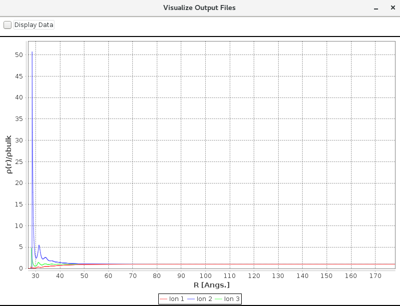
a)b)

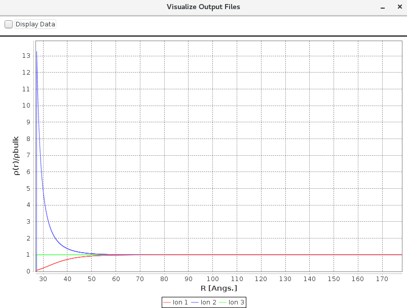
Figure 19: Example4: Ionic and water density distribution. Left and right plots correspond to CSDFT and NLPB, respectively.

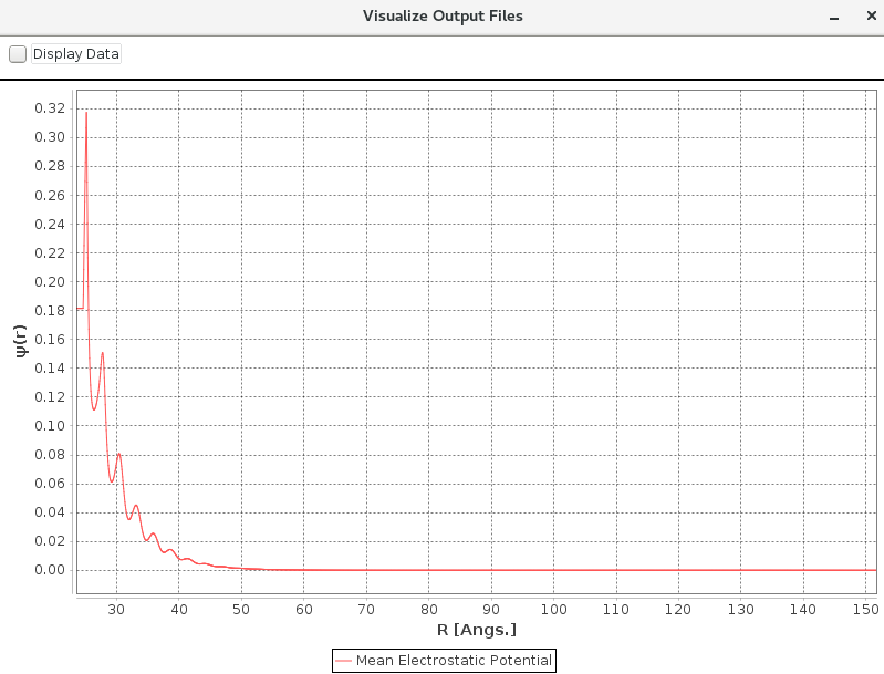
a)b)

Figure 20: Example5: Mean electrostatic potential. Left and right plots correspond to CSDFT and NLPB, respectively.

Overall, the software offers diversity in applicability and analysis on many colloidal systems. For instance, running multiple simulations at different pH levels may provide a molecular understanding on the impact of pH on the ZP, SCD, and EDL properties of macroions, and consequently, their stability and aggregation. Furthermore, simulating different electrolyte solutions may be useful to understand the effects of biological fluids on biomolecules and their functions. It is also possible to perform multiple simulations for different macroion sizes, charges and shapes to study their influence on membrane absorption.

V Future Directions

Users will be notified to update the software when a new release is available. Additional features to be included in coming releases are: 1) modeling more complex charging mechanism on the surface of nanomaterials including more than one active functional group and the release /adsorption of ions; 2) modeling solvent polarization effects key-23 . Future work will be focused on modeling: 1) inhomogenous surface charge density and solutes with irregular shapes; 2) nanomaterials having surface functionalization; 3) ionic currents along biopolymerskey-13 .

APPENDIX A: Theory and Numerical Scheme

.1 CSDFT for Spherical and Cylindrical macroions immersed in a aqueous electrolyte solution at neutral pH.

In this approach, we consider a rigid charged macroion of effective radius $R$ and uniform surface charge density $\sigma$ surrounded by an electrolyte solution comprised of $m$ ionic species. We use the solvent particle model to characterize the electrolyte. Each ionic species $i$ is represented by bulk Molar concentration $[\rho_{i}^{0}]$, a charged hard sphere of diameter $d_{i}$, and total charge $q_{i}=ez_{i}$, where $e$ is the electron charge and $z_{i}$ is the corresponding ionic valence. Additionally, the solvent molecules are represented as a neutral ion species whereas the solvent electrostatics is considered implicitly by using the continuum dielectric environment with a dielectric constant $\epsilon$. The macroion-liquid interaction induces inhomogeneous ion profiles $\left[\rho_{i}(r)\right]$ which are calculated using CSDFT as follows key-12 ; key-14 :

$$\left[\rho_{i}(r)\right]=\Bigg{\{} \begin{aligned} \left[\rho_{i}^{0}\right]exp\{\Delta E_{i}(r,\{[\rho_{j}])\},&r>R+d_{i}/2\\ 0,&r\leq R+d_{i}/2\end{aligned}$$ (1)

where $\Delta E_{i}(r,\{[\rho_{j}])\equiv-\beta q_{i}\psi(r,\{[\rho_{j}]\})+\Delta c_{i}^{(1)hs}(r;\{[\rho_{j}]\})+\Delta c_{i}^{(1)res}(r;\{[\rho_{j}]\})$ stands for the ionic PMF per unit of thermal energy $KT$, $\beta=1/kT$ , $k$ is the Boltzmann constant, $T$ the temperature, and $c_{i}^{(1)hs}(r;\{[\rho_{j}]\})$ and $c_{i}^{(1)res}(r;\{[\rho_{j}]\})$ are the hard sphere (particle crowding) and residual electrostatic ion-ion correlation functions, respectively. $\psi(r,\{[\rho_{j}]\})$ represents the MEP of the system

$$\psi(r,\{[\rho_{j}]\})=\frac{e}{\mbox{$\epsilon$}}\int_{r}^{\infty}\frac{dr^{\prime}}{r^{\prime}}P(r^{\prime},\{[\rho_{j}]\},n)$$ (2)

and

$$P(r^{\prime},n)=\frac{1}{r^{\prime n-1}}\left\{\frac{R^{n}\sigma}{e}+\int_{R}^{r^{\prime}}dr^{\prime}r^{\prime n}\sum_{i}z_{i}\rho_{i}(r^{\prime})\right\}\quad\left\{\begin{array}[]{c}\textrm{n=1 for cylindrical macroions}\\ \textrm{n=2 for spherical macroions}\end{array}\right.$$ (3)

the integrated charge (see Figure 1). Expression (2) is the formal solution of the PB equation for an homogeneous anisotropic dielectric media $\epsilon$

$$\begin{array}[]{c}\nabla^{2}\psi(r,\{[\rho_{j}]\})=-\frac{1}{\epsilon}\sum_{i=1}^{m}z_{i}\left[\rho_{i}(r)\right]\}\\ \\ \epsilon\partial\psi(r,\{[\rho_{j}]\})/\partial r|_{r=s}=-\sigma,\qquad\psi(r,\{[\rho_{j}]\})|_{r\rightarrow\infty}\rightarrow 0,\end{array}$$ (4)

with the surface charge layer position defined as $s\equiv R+<\{d_{i}\}>$ and $<\{d_{i}\}>\equiv N_{A}l_{B}^{3}\sum_{i}\left|z_{i}\right|[\rho_{i}^{0}]d_{i}/(2m)$. In the latter definition $N_{A}$ and $l_{B}$ stand for the Avogadro number and the Bjerrum length, respectively.

.2 Surface Complexation Model: Accounting for pH Effects of the Electrolyte aqueous Solution on the macroion Surface Charge Density

In order to account for the titration that regulates the macroion surface charge density $\sigma$ we consider the following two protonation reactions of single MO-coordinated sites :

$$MOH\leftrightarrow MO^{-}+H^{+},\qquad MOH+H^{+}\leftrightarrow MOH_{2}^{+}.$$ (5)

with equilibrium constants $K_{A}$ and $K_{B}$

$$K_{A}=\frac{N_{MO^{-}}[H^{+}]_{s}}{N_{MOH}},\qquad K_{B}=\frac{N_{MOH_{2}^{+}}}{N_{MOH}[H^{+}]_{s}}.$$ (6)

In the above expressions, $N_{MOH}$, $N_{MO^{-}}$, and $N_{MOH_{2}^{+}}$ are the surface site densities of $MOH$, $SO^{-}$ and $MOH_{2}^{+}$, respectively. $[H^{+}]_{s}$ is the concentration of $H^{+}$ ions at the SCD position $s$, namely

$$[H^{+}]_{s}\equiv\left[\rho_{H}(s)\right]=[\rho_{H}^{0}]exp\{\Delta E_{H}(s,\{[\rho_{j}])\},$$ (7)

where $\Delta E_{H}(s,\{[\rho_{j}])=-\beta\zeta+\Delta c_{H}^{(1)hs}(s;\{[\rho_{j}]\})+\Delta c_{H}^{(1)res}(s;\{[\rho_{j}]\})$ is the hydrogen PMF per unit of thermal energy $KT$, $\zeta\equiv\psi(s,\{[\rho_{j}]\})$ is the ZP, and $\Delta c_{H}^{(1)hs}$ and $\Delta c_{H}^{(1)res}$ represent the hydrogen hard sphere (particle crowding) and ion-ion correlation contributions, respectively. The bulk concentration of $H^{+}$ ions is represented by $[\rho_{H}^{0}]$, which is related to the $pH$ value of the bulk liquid at infinite dilution by the expression $pH=-Log([\rho_{H}^{0}])$. The total number density of functional groups on the SCD position is $N_{total}=N_{MO^{-}}+N_{MOH}+N_{MOH_{2}^{+}}$ and the SCD is $\sigma=-F(N_{MO}-N_{MOH_{2}^{+}})$, where $F$ represents the Faraday constant . Writing the densities sites in terms of the equilibrium constants (7), the SCD can be calculated as follows key-15 ; key-16 :

$$\sigma=-FN_{total}\frac{K_{A}-K_{B}\left[\left[\rho_{H}(r)\right]_{r=s}\right]^{2}}{K_{A}+\left[\rho_{H}(r)\right]_{r=s}+K_{B}\left[\left[\rho_{H}(r)\right]_{r=s}\right]^{2}}$$ (8)

The $pH$ of the solution is adjusted by adding strong acid ($NaOH$) and ($HCl$) solutions to the electrolyte. The free proton and hydroxyl ion bulk concentrations are given by the well-known expressions $[\rho_{H}^{0}]=10^{-pH},\quad and\quad[\rho_{OH}^{0}]=10^{-(14-pH)},$ respectively, and the bulk concentrations of the electrolyte are chosen to satisfy the bulk electroneutrality condition.

.3 NLPB approach

NLPB is a particular case of the CSDFT approach. Indeed, the expressions introduced in previous sections for CSDFT recover the NLPB approach by setting all ion sizes equal to zero. In particular, $s=R$, $\Delta c_{i}^{(1)res}(r;\{[\rho_{j}]\})=0,$ and $\Delta c_{i}^{(1)hs}(r;\{[\rho_{j}]\})=0$ in continuum models.

.4 Iterative Solver Scheme

Note that expression (8) describes the effects of the structural and electrostatic properties of the electrolyte on the SCD, whereas the boundary condition in expression (4) accounts for the SCD effects on the structural and electrostatic properties of the electrolyte. Therefore, eqns (1)-(8) must be solved self-consistently as it is shown in Figure 21.

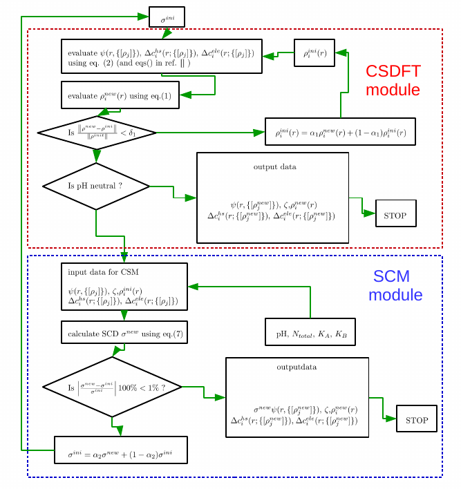
Figure 21: Iterative Solver Scheme

References

- (1) Gerald S. Manning. The molecular theory of polyelectrolyte solutions with applications to the electrostatic properties of polynucleotides. Quarterly Reviews of Biophysics, 11(2):179– 246, 1978.
- (2) David C. Grahame. The electrical double layer and the theory of electrocapillarity. Chemical Reviews, 41(3):441–501, 1947. PMID: 18895519.
- (3) John Newman. Electrochemical Systems, chapter 1. Englewood Cliffs, N.J. Prentice-Hall, 1973.
- (4) M. Barisik, S. Atalay, A. Beskok and S.J. Qian, J. Phys. Chem. C 2014, 118, 1836.
- (5) Sonnefeld, M. Löbbus and W. Vogelsberger, Colloids Surf. A, 2001, 195 215.
- (6) J.H. Masliyah and S. Bhattacharjee, Electrokinetic and Colloid Transport Phenomena, John Wiley and Sons, Hoboken, 2006.
- (7) A. Studart, E. Amstad and L. Gauckler, Langmuir 2007, 23, 1081.
- (8) Paul A. Janmey, David R. Slochower, Yu-Hsiu Wang, Qi Wen, and Andrejs Cebers. Polyelectrolyte properties of filamentous biopolymers and their consequences in biological flu- ids. Soft Matter, 10:1439–1449, 2014.
- (9) Alexei A. Kornyshev. Double-layer in ionic liquids: Paradigm change? Physical Chemistry B, 111(20):5545 – 5557, 2007.
- (10) Ren, P., Chun, J., Thomas, D.G., Schnieders, M.J., Marucho, M., Zhang, J. and Baker, N.A., Quarterly Reviews of Biophysics, 2012), 49, 427.
- (11) N. A. Baker, D. Bashford and D. A. Case, New Algorithms for Macromolecular Simu- lation, 2006, 49, 263.
- (12) Ovanesyan, Z.; Medasani, B.; Fenley, M. O.; Guerrero-García, G. I.; Olvera de la Cruz, M. and Marucho, M. (2014). Excluded volume and ion-ion correlation effects on the ionic atmosphere around B-DNA: Theory, simulations, and experiments, J Chem Phys 141 : 225103 (PMCID: PMC4265039).
- (13) Christian Hunley, Diego Uribe, and Marcelo Marucho, A Multi-scale approach to describe electrical impulses propagating along Actin filaments in both intracellular and in-vitro conditions, submitted to RCS Advances.
- (14) Medasani, B.; Ovanesyan, Z.; Thomas, D. G.; Sushko, M. L. and Marucho, M. (2014). Ionic asymmetry and solvent excluded volume effects on spherical electric double layers: A density functional approach, J Chem Phys 140 : 204510 (PMCID: PMC4039739).
- (15) Ovanesyan, Z.; Aljzmi, A.; Almusaynid, M.; Khan, A.; Valderrama, E.; Nash, K. L. and Marucho, M. (2016). Ion-ion correlation, solvent excluded volume and pH effects on physicochemical properties of spherical oxide nanoparticles, J Colloid Interface Sci 462 : 325-333
- (16) Hunley, C. and Marucho, M. (2017). Electrical double layer properties of spherical oxide nanoparticles, Phys. Chem. Chem. Phys. 19 : 5396-5404
- (17) Jmol: an open-source Java viewer for chemical structures in 3D. http://www.jmol.org/
- (18) Chen, C.R., and Makhatadze, M. ProteinVolume: calculating molecular van der Waals and void volumes in proteins, , BMC Bioinformatics 2015 16:101.
- (19) Voss, N.R, and Gerstein, M., 3V: cavity, channel and cleft volume calculator and extractor, Nucleic Acids Res. 2010 July 1; 38 W555–W562
- (20) Dolinsky TJ, Nielsen JE, McCammon JA, Baker NA. PDB2PQR: an automated pipeline for the setup, execution, and analysis of Poisson-Boltzmann electrostatics calculations. Nucleic Acids Research 32 W665-W667 (2004).
- (21) http://www.poissonboltzmann.org/
- (22) Vergara-Perez, S. and Marucho, M. (2016). MPBEC, a Matlab Program for Biomolecular Electrostatic Calculations, Comput. Phys. Commun. 198 : 179-194
- (23) R. D. Shannon (1976). "Revised effective ionic radii and systematic studies of interatomic distances in halides and chalcogenides". Acta Crystallogr A. 32: 751–767.
- (24) Warshavsky, V. and Marucho, M. (2016). Polar-solvation classical density-functional theory for electrolyte aqueous solutions near a wall, Phys Rev E 93 : 042607