Optimizing Prediction Intervals by Tuning Random Forest via Meta-Validation

Abstract

Recent studies have shown that tuning prediction models increases prediction accuracy and that Random Forest can be used to construct prediction intervals. However, to our best knowledge, no study has investigated the need to, and the manner in which one can, tune Random Forest for optimizing prediction intervals – this paper aims to fill this gap. We explore a tuning approach that combines an effectively exhaustive search with a validation technique on a single Random Forest parameter. This paper investigates which, out of eight validation techniques, are beneficial for tuning, i.e., which automatically choose a Random Forest configuration constructing prediction intervals that are reliable and with a smaller width than the default configuration. Additionally, we present and validate three meta-validation techniques to determine which are beneficial, i.e., those which automatically chose a beneficial validation technique. This study uses data from our industrial partner (Keymind Inc.) and the Tukutuku Research Project, related to post-release defect prediction and Web application effort estimation, respectively. Results from our study indicate that: i) the default configuration is frequently unreliable, ii) most of the validation techniques, including previously successfully adopted ones such as 50/50 holdout and bootstrap, are counterproductive in most of the cases, and iii) the 75/25 holdout meta-validation technique is always beneficial; i.e., it avoids the likely counterproductive effects of validation techniques.

1 Introduction

One important phase of software development is release planning ruhe2010product. During release planning, stakeholders define characteristics of the software release such as the requirements to implement, the defects to fix, the developers to use, the amount and type of testing, and the release duration. The project manager must make decisions in the midst of conflicting goals like time-to-market, cost, number of expected defects, and customer demands. These business goals, their importance, and clients’ expectations vary among releases of the same or different projects, and in turn the number of acceptable defects varies. For instance, some projects are more safety critical than others and, therefore, can tolerate fewer defects. Thus, the manager might decide to increase the amount of testing, reduce the number of features, or postpone the release deadline if the predicted number of defects does not fit the business goals of that project release.

In 2011, Keymind developed and institutionalized a tool to help managers define characteristics of a software release according to the predicted number of post-release defects. Over the last seven years, the tool was subject to eight major upgrades. Each upgrade included refreshing the data (i.e., collecting data about new software releases), refreshing the type of data (i.e., adding metrics based on changes in technologies being used), improving the usability of the layout, and selecting the most accurate prediction models. A major improvement effort took place in 2013, when Keymind transitioned from predicting the number of defects to predicting the upper bounds related to a confidence level falessi2014achieving. Thus, Keymind moved from supporting a sentence such as “The expected number of defects is $y$” to supporting a sentence such as “We are 90% confident that the number of defects is less than $y$.” Then, during a discussion with the Keymind team in 2016, we learned that the current model was actionable but not fully explicative. Specifically, we realized that an interval is more informative than its upper-bound, i.e., the lower bound is also informative. For instance, there is a practical difference in the intervals $0\leq y\leq 10$ and $9\leq y\leq 10$ constructed for two different software projects. On the one hand, the former is more desirable as the actual number of post-release defects could be 0, i.e., spending additional money on testing might not be required. On the other hand, the latter is more actionable, i.e., there is less variability. Upon reviewing the literature, we determined that prediction intervals can be used to support the sentence “We are 90% confident that the number of defects is between $a$ and $b$”, where $a$ and $b$ are the lower and upper bounds of the prediction interval jorgensen2003effort; angelis2000simulation; jorgensen2002combination.

1.1 Definitions

In order to avoid ambiguities in the remainder of this paper, we define the following key terms and concepts.

• Model: a formal description of structural patterns in data used to make predictions (e.g., Random Forest) witten2016data.

• Parameter: an internal variable of the algorithm used to learn the model (e.g., MTRY witten2016data).

• Configuration: the set of values for each of the parameters of a model (e.g., MTRY=1.0 and all other parameters set as default).

• Prediction Interval (PI): an estimate of an interval, with a certain probability, in which future observations will fall (e.g., $0\leq\text{post-release defects}\leq 5$) geisser1993predictive. An important difference between the confidence interval (CI) and the PI is that the PI refers to the uncertainty of an estimate, while the CI refers to the uncertainty associated with the parameters of a distribution jorgensen2003effort, e.g., the uncertainty of the mean value of a distribution of values.

• Width: the size of a PI. Width is computed as the upper bound minus the lower bound, e.g., $Width(0\leq y\leq 5)=5$. The smaller the width, the better.

  

  Figure 1: Data used for model evaluation, validation and meta-validation for tuning.

• Coverage: also called coverage probability, hit-rate, or actual confidence, is the proportion of time the true value falls within the PI dodge2006oxford. For instance, the true value might fall within the PI of a model 92% of the time. The higher the coverage, the better.

• Nominal Confidence (NC): the stated proportion of time the true value should fall within the PI dodge2006oxford. A project manager might like to have a model that constructs PI that contain the true value 90% of the times, i.e., the nominal confidence is 90%.

• Reliable: refers to a model that constructs PIs such that $Coverage\geq NC$. For instance, a model is said to be reliable if nominal confidence is 90% and coverage is 92%. Reliable models are preferable.

• Best Configuration: with respect to PI, the goodness of a configuration is (1) contingent upon reliability and (2) inversely proportional to width. Thus, we define the best configuration as the configuration with smallest width among the set of reliable configurations.

• Model evaluation: the process of measuring the performance of a model, as configured in a specific way (i.e., default configuration). Typically the model is first trained (i.e., learned) and then it is tested (i.e., accuracy is measured). For instance, in Figure 1, the dataset is first ordered chronologically and then split in two parts: train and test. Note that the proportion of train and test (i.e., 66/33) is consistent in fu2016tuning and tantithamthavorn2016automated. We also note that there are validation techniques that split the dataset in proportions other than 66/33 or that do not even preserve the order of the data between training and testing. We discuss validation techniques in further detail in Section 2.6.

• Tuning, auto-configuration, or configurations validation: is the process of automatically finding the model configuration which optimizes an objective function thornton2013auto; bergstra2011algorithms. In our context, we are interested in selecting the configuration which constructs the narrowest reliable PI. In this work, because we let only one parameter vary, and because we evaluate all possible values of said parameter, a tuning technique coincides with an exhaustive search and a specific validation technique. Thus, in this work, the terms tuning technique and validation technique can be used interchangeably. Tuning uses the training set of the model evaluation for validating candidate model configurations. Specifically, in Figure 1, the evaluation training set is divided into train^′ and test^′ of tuning. We note that train and test sets of tuning can be of different proportions; the only constraint of a tuning technique is that it is not exposed to the evaluation test set.

• Beneficial: refers to a tuning technique that is able to select a configuration that constructs PIs that are reliable and narrower than what the default configuration constructs.

• Configuration meta-validation: aka meta-validation, is the process of automatically finding the most beneficial tuning technique. In other words, if tuning selects the best configuration, by validating the different configurations, meta-validation selects the best technique to select the best configuration. Meta-validation uses the tuning training set for validating the tuning techniques. In Figure 1, the train^′ subset is further divided into train^′′ and test^′′. Again, training and test sets can have different proportions; the only constraint is that no meta-validation subset use test or test^′.

1.2 Motivation

In order to better understand the problem we are trying to solve, Figure 2 reports PIs at NC90 (green), NC95 (blue), and NC99 (yellow) as constructed by the default random forest configuration on the Keymind dataset. The model is trained on the first 66% of the data and PIs are constructed for the remaining 33%. We plot the actual number of post-release defects with the same color of the narrowest interval in which it is contained, e.g., a green point indicates that the actual value is contained in the PI constructed at NC90. We plot points that are not contained at any NC as red. Lastly, we plot the predicted value with a “x”.

In Figure 2, we observe that NC90 covers 89% (106), NC95 covers 95% (113), and NC99 covers 98% (117) of the total (119) releases. In other words, the default random forest configuration is not reliable at NC90 and NC99. Thus, we cannot use the default configuration to support the claim “We are NC% confident that the number of defects is between a and b” if NC is 90 or 99. This motivates the need for tuning to choose a configuration, other than default, which constructs reliable PIs.

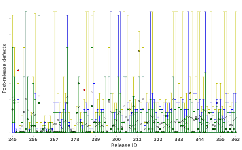
Figure 2: Prediction intervals at NC90 (green), NC95 (blue), and NC99 (yellow) as constructed by the default random forests configuration on the Keymind dataset. The model is trained on the first 66% of the data and PIs are constructed for the remaining 33%.

Figure 2 is also useful to identify the differences between PIs and CIs. Specifically, there are cases in which the NC95 and NC99 intervals cannot be seen (e.g., release 252). This means that the intervals constructed at all NCs are equivalent. This denotes a significant difference between PIs and CIs: the width of CIs is strongly correlated with NC. Moreover, within the same NC, higher upper bounds do not always correspond with more predicted defects. For example, release 280 has a higher number of predicted defects than release 267 but a lower upper bound at NC95 and NC99. This denotes another significant difference between PIs and CIs. Specifically, within the same NC, the upper bound of CIs is strongly correlated with the predicted number (i.e., NC50).

Finally, it is interesting to note that larger intervals do not always correspond with more actual defects. For example, release 248 has the second most defects and the 27th, 33rd, and 47th largest interval for NC90, NC95, and NC99, respectively.

1.3 Aim

Recent studies have shown that tuning prediction models increases accuracy duan2003evaluation; di2011genetic; corazza2013using; borg2016tuner; fu2016tuning, and that Random Forest can be used to to predict defect and effort data Moeyersoms:2015; DBLP:journals/iee/SatapathyAR16 and to construct prediction intervals. However, to our best knowledge, no study has investigated the need, or how, to tune Random Forest for optimizing prediction intervals; this paper aims to fill this gap.

The contribution of this paper is threefold;

1. We use Random Forest to construct prediction intervals for software engineering data (fault and effort).

2. We present and evaluate the use of eight validation techniques for tuning to determine which are beneficial.

3. We present and evaluate three meta-validation techniques to determine which are beneficial, i.e., which automatically choose a beneficial validation technique.

Specifically, we investigate the following research questions.

RQ 1

Is default the best configuration?

RQ 2

Are validation techniques beneficial?

RQ 3

Are meta-validation techniques beneficial?

Our validation uses data from our industrial partner (Keymind Inc.) and the Tukutuku Research Project, containing 363 and 195 industrial data points related to post-release defect prediction and Web application effort estimation, respectively.

Results show that the default configuration is frequently unreliable and previously successfully adopted validation techniques, such as 50/50 holdout and bootstrap, are frequently counterproductive in tuning. Moreover, no single validation technique is always beneficial; however, the meta 75/25 holdout technique selects validation techniques that are always beneficial. Thus, results show that Random Forest is a viable solution to construct prediction intervals only if well tuned. Because no single validation technique resulted always beneficial, we recommend the use of meta 75/25 holdout meta-validation technique to dynamically chose the validation technique according to the dataset and prediction interval of interest.

In order to support the usability and replicability of this study, we provide a Python package for tuning and meta-tuning Random Forests PIs. We also show how to use it over a large open source project called Apache-ANT.

1.4 Structure

The remainder of the paper is structured as follows. Section 2 discusses related work. Section LABEL:sec:design describes our experimental design. Section LABEL:sec:results present results and discussion. Section LABEL:sec:replicability presents meta_tune, an open source Python package we developed for using and tuning prediction intervals. Section LABEL:sec:threats discusses threats to validity. Section LABEL:sec:conclusion concludes the paper and identifies areas for future work.

2 Related Work

2.1 Defect Prediction

Numerous recent studies have applied data mining and machine learning techniques to improve QA resource allocation, i.e., to focus QA efforts on artifact(s) expected to be the most defective. These studies can be generally categorized as defect classification (i.e., the artifact is either defective or not defective) kim2011dealing; rahman2013sample; herzig2013s; zhang2014towards; mishra2012defect; selvaraj2013support; kim2008classifying; aversano2007learning; zimmermann2007predicting; menzies2013local; okutan2014software; guo2004robust; menzies2010defect; minku2015make; turhan2009relative; menzies2011local; suffian2014prediction; giger2012method; padberg2002empirical or defect prediction (i.e., the artifact contains n defects) li2003selecting; petersson2004capture; thelin2002confidence; biffl2001evaluating; biffl2000using; thelin2004team.

Similar to this paper, li2003selecting investigate the use of post-release defect prediction in the planning of widely used multi-release commercial systems. They conclude that models currently available fall short because they do not adequately consider organizational changes and customer adoption characteristics.

A family of studies apply capture-recapture to defect prediction petersson2004capture; thelin2002confidence; biffl2001evaluating; thelin2004team; padberg2002empirical. These studies estimate the remaining number of defects by analyzing characteristics of the overlapping set of defects detected by multiple, independent reviewers. Capture-recapture was first applied to software inspections by eick1992estimating in 1992 and petersson2004capture provide a survey of the method.

2.2 Effort Prediction

It is often difficult to predict the amount of effort required to complete a software project due to changes associated with aspects of software development (e.g., requirements, development environments, and personnel). It is of practical importance to have accurate effort predictions as it affects project management and resource allocation, i.e., larger parts of the budget should be allocated for artifacts that are expected to require more effort. Software effort prediction has been the subject of numerous studies, as summarized by boehm2000software and molokken2003review.

jorgensen2002combination use independent expert opinions to predict the amount of development effort. They suggest that it is better to have estimation teams comprising several different types of roles, rather than estimation teams consisting of only technical roles, to help reduce systematic bias. We incorporate this suggestion into the development of the Keymind dataset, which we discuss further in Section LABEL:sec:design_keymind.

briand1998cobra develop and apply CoBRA, a hybrid method which combines aspects of algorithmic and experiential approaches, to predicting the cost of software development. To construct CoBRA, domain experts are asked to decide the causal factors and their possible values. Experimental results show realistic uncertainty estimates. However, this method requires, and is sensitive to, human estimates.

di2011genetic propose and validate the use of a Genetic Algorithm with a grid search for tuning support vector regression for estimating defective file. corazza2013using propose and validate a meta-heuristics Tabu Search for tuning support vector regression for point values effort estimation. Their results show that Tabu search outperformed other simpler approaches, such as random configuration and default configuration. Because in this work it is reasonable to tune only one parameter, then a full search is preferable to any other incomplete search such as the Genetic or Tabu types.

Whigham:2015:BMS: propose a baseline for comparing effort estimation models. Unfortunately such a baseline does not apply to prediction interval and therefore cannot be used in this work.

To the best of our knowledge, there has been no study that has applied Random Forest to effort prediction.

2.3 Intervals in Software Engineering

Predictions about the number of post-release defects or development effort are intrinsically uncertain. This uncertainty primarily arises as a result of the nature of software development (e.g., changing requirements, unstable development teams and environments). However, there is also some degree of uncertainty associated with the model used to make the prediction. Hence, information about the level of uncertainty is desirable.

Software engineering studies using intervals can be generally categorized as either using CIs in combination with capture-recapture methods padberg2002empirical; petersson2004capture; thelin2002confidence; thelin2004team, or constructing PIs from expert opinion elicitation jorgensen2002combination, bootstrapping angelis2000simulation, regression models braga2007software, a combination of cluster analysis and classification methods bakir2011comparative,a multi-objective evolutionary algorithm sarro2016multi, or based on prior estimates jorgensen2003effort. We note that linear regression is not typically used in the construction of prediction intervals with respect to software engineering predictions. In our case, our datasets violated multiple assumptions of linear regression such as normality and homoscedasticity; thus, we did not consider it as a viable approach.

thelin2002confidence show that model-based point estimates, when used with confidence intervals, outperform human-based estimates. This result is particularly relevant as previous studies conclude that human-based estimates outperform model-based point estimates.

vander1993assessing evaluate Walds Likelihood CI and Mh–JK CIs and conclude that the Walds Likelihood CI includes the correct number of defects in most cases, and therefore should be preferred over Mh-JK. However, the Walds Likelihood CI is often too conservative, which leads to large intervals petersson2004capture.

Notably, angelis2000simulation describe an instance-based learning approach used in combination with bootstrapping to construct effort intervals. They claim to construct CIs, however, our reading of the paper suggests they actually construct PIs.

jorgensen2003effort introduce an approach used to construct effort PI based on the assumption that they are able to select prior projects with similar estimation errors to that of a future project, i.e., the selected projects must have similar degrees of uncertainty as the future project.

Regarding PI construction via expert-opinion elicitation, jorgensen2002combination use human-based PIs in effort estimation and conclude that group-discussion based PIs are more effective than “mechanically” combining individual PIs. However, the approach they put forth requires significant time and effort on the part of the experts involved and is sensitive to the accuracy of human estimates. Further, PIs based on human estimates tend to be too narrow to reflect high confidence levels (e.g., 90% nominal confidence) jorgensen2004better; connolly1997decomposed.

In conclusion, despite significant research advances in predictive models for software analytics, there have been very few studies that investigate the use of model-based intervals (CI or PI). A majority of those that have rely on capture-recapture methods petersson2004capture; thelin2002confidence; biffl2001evaluating; thelin2004team; padberg2002empirical, which are a very specific type of prediction and have the distinct disadvantage of requiring human review. Methods relying on human estimates thelin2002confidence; jorgensen2002combination; briand1998cobra are infeasible in our context. To our knowledge, no SE studies have investigated constructing PIs with Random Forest.

2.4 Random Forest

Decision trees are attractive for their execution time and the ease with which they can be interpreted. However, decision trees tend to overfit and generalize poorly to unseen data witten2016data. The Random Forest (RF), first introduced in 1995 by Tin Kam Ho ho1995random, is an example of ensemble learning in which multiple decision trees are grown independently.

Given data-points $D_{i}$ and responses $y_{i}$, $i=1,\dots,m$, each decision tree is grown from a bootstrapped sample of D. Further, only a random subset of predictors is considered for the split of each node breiman2001random. The number of predictors to consider at each split is specified by the parameter MTRY.

Thus, the trees grown in different, random subspaces generalize in a complementary manner, and their combined decision can be monotonically improved ho1995random; breiman2001random. Given data-points $D_{i}$ and responses $y_{i}$, $i=1,\dots,m$, where each $D_{i}$ contains $n$ predictors, each tree in the RF is grown as follows:

• Construct the training set by sampling, with replacement, m data-points from D.

• At each node, $n\textprime=n\times MTRY$ predictors are selected randomly and the most informative of these n´ predictors is used to split the node.

• Each tree is grown to the largest extent possible.

The prediction $\hat{y}$ of a single tree $T$ for a new data-point $\vec{X}=\vec{x}$ is obtained by averaging the observed values $\ell(\vec{x})$, where $\ell$ is the leaf that is reached when dropping $\vec{x}$ down $T$.

The prediction of a Random Forest $\hat{y}$ is equivalent to the conditional mean $\hat{\mu}(\vec{x})$ which is approximated by averaging the prediction of the $k$ trees breiman2001random:

$$\hat{y}=\hat{\mu}(\vec{x})=k^{-1}\sum_{i=1}^{k}\ell_{k}(\vec{x}).$$ (1)

guo2004robust were the first to investigate the use of RF in defect classification. They conclude that RF outperforms the logistic regression and discriminant analysis of SAS, the VF1 and VotedPerceptron classifiers of WEKA, and NASA’s ROCKY menzies2003can.

2.5 Random Forest Prediction Intervals

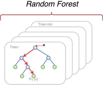
Figure 3: Random Forest overview.

A common goal in statistical analysis is to infer the relationship between a response variable, $Y\in\mathbb{R}$, and a predictor variable $\vec{X}$. Given $\vec{X}=\vec{x}$, typical regression analysis determines an estimate $\hat{\mu}(\vec{x})$ of the conditional mean of $Y$. However, the conditional mean describes just one aspect of the relationship, neglecting other features such as fluctuations around the predicted mean meinshausen2006quantile. In general, given $\vec{X}=\vec{x}$ the distribution function is defined by the probability that $Y\leq y$ evans2000statistical:

$$F(y|\vec{x})=P(Y\leq y|\vec{X}=\vec{x}).$$ (2)

For a continuous distribution, the $\tau$-quantile is defined such that $\tau=F(y|\vec{X}=\vec{x})$ meinshausen2006quantile:

$$Q_{\tau}(\vec{x})=inf\{y:F(y|\vec{X}=\vec{x})\geq\tau\}.$$ (3)

We can use these definitions to construct PIs. For instance, the 90% prediction interval is given by:

$$I_{.90}(\vec{x})=[Q_{.05}(\vec{X}=\vec{x}),Q_{.95}(\vec{X}=\vec{x})]$$ (4)

In other words, there is a 90% probability that a new observation of $Y$ is contained in the interval. meinshausen2006quantile presents the Quantile Regression Forest (QRF), a general method for constructing prediction intervals based on decision trees. Rather than approximating the conditional mean, he shows that the responses from each tree $T_{i}$, $i=1,\dots,k$ can be used to approximate the full conditional distribution function $\hat{F}(y|\vec{X}=\vec{x})$.

We can use the RF to construct prediction intervals if we ensure that all trees are fully expanded, i.e., each leaf has only one response. For a given $\vec{X}=\vec{x}$ and RF with trees $T_{i}$, $i=1,\dots,k$, the distribution function can be approximated as:

$$\hat{F}(y|\vec{x})=k^{-1}\sum_{i=1}^{k}1_{\{\ell_{i}(\vec{x})\leq y\}}.$$ (5)

In other words, the likelihood that the prediction $\hat{y}_{i}=\ell_{i}(\vec{x})$ is less than or equal to the response $y$. Then, the $\tau$-quantile can be approximated as:

$$\hat{Q}_{\tau}(\vec{x})=inf\{y:F(y|\vec{X}=\vec{x})\geq\tau\}.$$ (6)

Finally, the 90% prediction interval can be approximated as:

$$\hat{I}_{.90}(\vec{x})=[\hat{Q}_{.05}(\vec{X}=\vec{x}),\hat{Q}_{.95}(\vec{X}=\vec{x})].$$ (7)

We note that it is possible that we are unable to fully expand all of the trees. This can happen if (1) the node is already pure, or (2) the node cannot be split further, i.e., all remaining data-points have the same predictors. In the former case, we know the response and the leaf size, i.e., we can still determine the conditional distribution. In the latter case, we do not know what the response would be if the node is split further; hence, we are unable to determine the conditional distribution. Lastly, we note that fully-expanding trees can lead to overfitting, in which case the intervals will provide little practical value meinshausen2006quantile. However, fully expanding trees is what breiman2001random suggests. Further, even if individual trees overfit, the effect should be mitigated by increasing the total number of trees in the forest.

Algorithm 1 Random Forest Prediction Intervals

1:procedure PredictionIntervals($D$, $y$, $nc$, $ph$)

2:     $\textit{D\_train},\textit{D\_test},\textit{y\_train},\textit{y\_test}\leftarrow\text{split(D, y, ph)}$

3:     $\textit{clf}\leftarrow\text{RandomForestRegressor()}$

4:     clf.fit(D_train, y_train)

5:

6:     $preds\leftarrow[[]]$

7:     for all est in clf.estimators do

8:         for all n, leaf in est.apply(D_test) do

9:              if leaf is not pure then

10:                  exit               

11:              $\textit{preds[n]}.extend(\textit{leaf.responses()})$               

12:

13:     $\alpha\leftarrow\frac{1-nc}{2}$

14:     $\beta\leftarrow 1-\alpha$

15:     $intervals\leftarrow[]$

16:     for all pred in preds do

17:         $intervals.append((Q_{\alpha}(pred),Q_{\beta}(pred)))$      

18:     return intervals

19:

20:procedure 

We present the procedure for constructing prediction intervals in Algorithm 1. The procedure accepts four arguments: D (the data-points), y (the responses), nc (the nominal confidence), and ph (the percent to be held out). In lines 2-4 we partition the data into training and test sets and learn a RF. In lines 7-11 we record the responses of all decision trees for each $d_{i}\in D_{test}$. We ensure that each leaf is pure on line 10. Finally, we construct prediction intervals on line 17.

Table 1 presents the list of parameters for Sci-Kit Learn’s RandomForestRegressor.

Table 1: Sci-Kit Learn RandomForestRegressor parameters

feature	description	value
n_estimators	The number of trees in the forest.	1000
max_features	The size of the subset of the features to consider for each split.	1.0*
max_depth	The maximum depth of the tree.	None
min_samples_ split	The minimum number of samples required to split an internal node.	2
min_samples_ leaf	The minimum number of samples required to be at a leaf node.	1
min_weight_ fraction_leaf	The minimum weighted fraction of the sum total of weights (of all the input samples) required to be at a leaf node.	0
max_leaf_nodes	If specified, trees are grown with the specified number of leaves in a best first fashion.	None
min_impurity_ split	Threshold for stopping early tree growth.	1E-7

2.6 Validation Techniques

Validation techniques (also referred to as performance estimation techniques) are methods used for estimating performance of a model on unseen data. They are widely used in the machine learning domain to compare the performance of multiple models on a dataset in order to select the most well suited model (i.e., the model that minimizes the expected error) d2012evaluating; lessmann2008benchmarking; myrtveit2005reliability.

Within the context of validating defect prediction models, tanti2017empirical report 89 studies (49%) use k-fold cross-validation, 83 studies (45%) use holdout validation, 10 studies (5%) use leave-one-out cross-validation, and 1 study (0.5%) uses bootstrap validation.

Validation techniques are also used in hyper-parameter optimization, i.e., tuning the parameters of a model tantithamthavorn2016automated; fu2016tuning. There are many validation techniques that can be applied and no consensus on which technique is the most effective beleites2005variance; braga2004cross; breiman1992submodel; kocaguneli2013software; kohavi1995study; mockus2000predicting; tanti2017empirical.

To our knowledge, only two techniques have been used in tuning models for software analytics: fu2016tuning use the holdout and tantithamthavorn2016automated use bootstrap. These studies serve as inspiration for this work; we analyze the two techniques used in their studies and include an additional six more. Moreover, we reuse part of their experimental design: we holdout one third of the initial dataset for testing. One of the major differences in this paper is that both our datasets contain data-points measured across multiple industrial projects and multiple releases of the same project, whereas each of their datasets contain data-points measured from a single release of an open-source project. Thus, our datasets are sensitive to time and this aspect could affect the performance of certain tuning techniques that do not preserve the dataset order (e.g., bootstrap) in learning and testing.

2.6.1 Order Preserving

Techniques which preserve the order of the dataset are commonly used for performance estimation with time-series data (e.g., forecasting) bergmeir2012use. We analyze five such techniques: time series cross-validation, time series HV cross-validation, and three variations of the non-repeated holdout. Given data-points $D_{i}$ and responses $y_{i}$, $i=1,\dots,m$:

H/k holdout partitions the dataset such that $\frac{h}{m}$ data-points are used for training and $\frac{k}{m}$ are used for testing. Holdout validation has the advantage of being faster than techniques which require multiple repetitions and is often acceptable to use if $D$ is sufficiently large witten2016data. However, it is criticized for providing unreliable estimates tanti2017empirical due to the fact that performance is estimated on a single subset of $D$. Further, the holdout is criticized as being statistically inefficient since much of the data is not used to train the model tanti2017empirical. Figure 1 provides an example of 66/33 holdout between validation-training and validation-testing.