KEK-TH-2029
Scale-invariant Feature Extraction of Neural Network
and Renormalization Group Flow

Abstract

Theoretical understanding of how deep neural network (DNN) extracts features from input images is still unclear, but it is widely believed that the extraction is performed hierarchically through a process of coarse-graining. It reminds us of the basic concept of renormalization group (RG) in statistical physics. In order to explore possible relations between DNN and RG, we use the Restricted Boltzmann machine (RBM) applied to Ising model and construct a flow of model parameters (in particular, temperature) generated by the RBM. We show that the unsupervised RBM trained by spin configurations at various temperatures from $T=0$ to $T=6$ generates a flow along which the temperature approaches the critical value $T_{c}=2.2{7}$. This behavior is opposite to the typical RG flow of the Ising model. By analyzing various properties of the weight matrices of the trained RBM, we discuss why it flows towards $T_{c}$ and how the RBM learns to extract features of spin configurations.

1 Introduction

Machine learning has attracted interdisciplinary interests as the core method of artificial intelligence, particularly of big data science, and is now widely used to discriminate subtle images by extracting specific features hidden in complicated input data. A deep neural network (DNN), which is motivated by human brains, is one of well-known algorithms [1]. Despite its enormous successes, it is still unclear why DNN works so well and how DNN can efficiently extract specific features. In discriminating images, we first provide samples of input images with assigned labels, such as a cat or a dog, and then train the neural network (NN) so as to correctly predict the labels of new, previously unseen, input images: this is the supervised learning and its ability of prediction depends on how much relevant features the NN can extract. On the other hand, in unsupervised learning algorithms, a NN is trained without assigning labels to data, but trained so as to generate output images that are as close to the input ones as possible. If the NN is successfully trained to reconstruct the input data, it must have acquired specific features of the input data. With this in mind, unsupervised learnings are often adopted for pre-training of supervised NNs.

How can DNN efficiently extract features? Specific features characteristic to input data usually have hierarchical structures. An image of a cat can still be identified as an animal in a very low resolution image but one may not be able to distinguish it from a dog. Thus it is plausible that depth of neural networks reflects such hierarchy of features. Namely DNN learns low-level (microscopic) characteristics in upper stream of the network and gradually extracts higher-level (macroscopic) characteristics as the input data flow downstream. In other words, the initial data will get coarse-grained towards output. This viewpoint is reminiscent of the renormalization group (RG) in statistical physics and quantum field theories, and various thoughts and studies are given [2, 3, 4, 5, 6, 7, 8, 9] based on this analogy. Especially, in a seminal paper [4], Mehta and Schwab proposed an explicit mapping between the RG and the Restricted Boltzmann Machine (RBM) [1, 10, 11, 12, 13, 14].

RG is the most important concept and technology to understand the critical phenomena in statistical physics and also plays an essential role to constructively define quantum field theories on lattice. It is based on the idea (and proved by Kenneth Wilson [15]) that the long-distant macroscopic behavior of a many body system is universally described by relevant operators (relevant information) around a fixed point, and not affected by microscopic details in the continuum limit. Through reduction of degrees of freedom in RG, the relevant information is emphasized while other irrelevant information is discarded. Particularly, suppose that the statistical model is described by a set of parameters $\{\lambda_{\alpha}\}$, and that the parameters are mapped to a different set $\{\tilde{\lambda}_{\alpha}\}$ by RG transformations. Repeating such RG transformations, we can draw a flow diagram in the parameter space of the statistical model,

$$\{\lambda_{\alpha}\}\rightarrow\{\tilde{\lambda}_{\alpha}\}\rightarrow\{\tilde{\tilde{\lambda}}_{\alpha}\}\rightarrow\cdots.$$ (1)

These RG flows control the behavior of the statistical model near the critical point where a second order phase transition occurs.

A simplest version of RBM is a NN consisting of two layers, a visible layer with variables $\{v_{i}=\pm 1\}$ and a hidden layer with variables $\{h_{a}=\pm 1\}$, that are coupled to each other through the Hamiltonian

$$\Phi(\{v_{i}\},\{h_{a}\})=-(\sum_{i,a}W_{ia}v_{i}h_{a}+\sum_{i}b_{i}^{(v)}v_{i}+\sum_{a}b_{a}^{(h)}h_{a})\,.$$ (2)

A probability distribution of a configuration $\{v_{i},h_{a}\}$ is given by

$$p(\{v_{i}\},\{h_{a}\})=\frac{1}{\cal Z}e^{-\Phi(\{v_{i}\},\{h_{a}\})}$$ (3)

where we defined the partition function by ${\cal Z}=\sum_{\{v_{i},h_{a}\}}e^{-\Phi(\{v_{i}\},\{h_{a}\})}$. No intra-layer couplings are introduced in the RBM. Now suppose that the RBM is already trained and the parameters of the Hamiltonian (2), namely $\{W_{ia},b_{i}^{(v)},b_{a}^{(h)}\}$, are already fixed through a process of training. The probability distribution $p(\{v_{i}\},\{h_{a}\})$ also provides the following conditional probabilities for $\{h_{a}\}$ (or $\{v_{i}\})$ with the other variables being kept fixed;

$$p(\{h_{a}\}|\{v_{i}\})=\frac{p(\{h_{a}\},\{v_{i}\})}{\sum_{\{h_{a}\}}p(\{h_{a}\},\{v_{i}\})}$$ (4)

$$p(\{v_{i}\}|\{h_{a}\})=\frac{p(\{h_{a}\},\{v_{i}\})}{\sum_{\{v_{i}\}}p(\{h_{a}\},\{v_{i}\})}\,.$$ (5)

These conditional probabilities generate a flow of distributions, and consequently a flow of parameters $\{\lambda_{\alpha}\}$ of the corresponding statistical model. Suppose that we have a set of $N(\gg 1)$ initial configurations $\{v_{i}=\sigma_{i}^{A}\}$ ($A=1,\ldots,N$), which are generated by a statistical model with parameters $\lambda_{\alpha}$, such as the Ising model at temperature $T$. In the large $N$ limit, the distribution function

$$q_{0}(\{v_{i}\})=\frac{1}{N}\sum_{A}\delta(v_{i}-\sigma_{i}^{A})$$ (6)

faithfully characterizes the statistical model with parameters $\lambda_{\alpha}$. Multiplying $q_{0}(\{v_{i}\})$ by the conditional probabilities (4) and (5) iteratively, we can generate a flow of probability distributions as

$$q_{0}(\{v_{i}\})\rightarrow r_{1}(\{h_{a}\})=\sum_{\{v_{i}\}}p(\{h_{a}\}|\{v_{i}\})q_{0}(\{v_{i}\})$$ (7)

$$r_{1}(\{h_{a}\})\rightarrow q_{1}(\{v_{i}\})=\sum_{\{h_{a}\}}p(\{v_{i}\}|\{h_{a}\})r_{1}(\{h_{a}\})$$ (8)

and so on for $q_{n}(\{v_{i}\})\rightarrow r_{n+1}(\{h_{a}\})$ and $r_{n+1}(\{h_{a}\})\rightarrow q_{n+1}(\{v_{i}\})$. Let us focus on Eq. (7). If the probability distribution $r_{1}(\{h_{a}\})$ is well approximated by the Boltzmann distribution of the same statistical model with different parameters $\tilde{\lambda}_{\alpha}$, we can say that the RBM generates a transformation from $\{\lambda_{\alpha}\}$ to $\{\tilde{\lambda}_{\alpha}\}$. If more than two layers are stacked iteratively, we can obtain a flow of parameters as in Eq. (1). Another way to obtain a flow is to look at the transformations $q_{0}(\{v_{i}\})\rightarrow q_{1}(\{v_{i}\})\rightarrow q_{2}(\{v_{i}\})\rightarrow\cdots$ and translate the flow of probability distributions into a flow of parameters $\{\lambda_{\alpha}\}.$ In the present paper, we consider the latter flow to discuss a relation with RG.

Mehta and Schwab [4] pointed out similarity between RG transformations of Eq. (1) and the above flows of parameters in the unsupervised RBM. But in order to show that the transformation of parameters $\{\lambda_{\alpha}\}$ in the RBM indeed generates the conventional RG transformation, it is necessary to show that the weight matrix $W_{ia}$ and the biases $b_{i}^{(v)},b_{a}^{(h)}$ of the RBM must be appropriately chosen so as to generate the correct RG transformation that performs coarse-graining of input configurations. In Ref.[4], multi-layer RBM is employed as an unsupervised-learning NN, and the weights and the biases are chosen by minimizing the KL divergences (relative entropy) between the input probability distribution and the reconstructed distribution by integrating (marginalizing) over the hidden variables. The authors suggested the similarity by looking at the local spin structures in the hidden variables, but they did not show it explicitly that the weights determined by the unsupervised learning actually generate the flow of RG transformations.

The arguments [4] and misconception in the literature are criticized by Ref.[6]. In a wider context, the criticism is related to the following question: what determines whether a specific feature of input data is relevant or not? In RG transformations of statistical models, long-wave length (macroscopic) modes are highly respected while short-wave length modes are discarded as noise. In this way, RG transformations can extract universal behavior of the model at long-wave length. But, of course, it is so because we are interested in the macroscopic behavior of the system: if we are instead interested in short-wave length physics, we need to extract opposite features of the model. Thus, we may say that extraction of relevant features needs pre-existing biases to judge, and supervised learning is necessary to give such biases to the machine. However this does not mean that unsupervised learnings do not have anything to do with the RG. Even in unsupervised learnings, a NN automatically notices and extracts some kind of features of the input data and the flow generated by the trained NN reflects such features.

In the present paper, we investigate relationship between the RBM and the RG by further studying the flows of distributions, Eqs. (7) and (8), that the unsupervised RBM generates. Here notice that in defining the flow of (7) and (8), we need to specify how we have trained the RBM because the training determines the properties of the weights and biases, and accordingly the behavior of the flow. In this paper we mostly use the following three different ways of trainings. One type of RBM (we call type V) is trained by configurations at various temperatures from low to high. Other two types (type H and L) are trained by configurations only at high (and only at low) temperatures. Then we translate these flows of probability distributions defined by Eqs. (7) and (8) into flows of temperature of the Ising model,

$$T\rightarrow\tilde{T}\rightarrow\tilde{\tilde{T}}\rightarrow\cdots.$$ (9)

In order to measure temperature, we prepare another NN trained by a supervised learning. The results of our numerical simulations lead to a surprising conclusion. In the type V RBM that has adequately learned the features of configurations at various temperatures, we found that the temperature approaches the critical point, $T\rightarrow T_{c}$, along the RBM flow. The behavior is opposite to the conventional RG flow of Ising model.

The paper is organized as follows. In section 2, we explain the basic settings and the methods of our investigations. We prepare sample images of the spin configurations of the Ising model, and train RBMs by the configurations without assigning labels of temperature. Then we construct flows of parameters (i.e., temperature) generated by the trained RBM. In section 3, we show various results of the numerical simulations, including the RBM flows of parameters. In section 4, we analyze properties of the weight matrices $W_{ia}$ using the method of singular value decomposition. The final section is devoted to summary and discussions. Our main results of the RBM flow and conjectures about the feature extractions of the unsupervised RBM are written in Sec. 3.2.

2 Methods

We explain various methods for numerical simulations to investigate relations between the unsupervised RBM and the RG of Ising model. Though most methods in this section are standard and well known, we explain them in details to make the paper self-contained. In Sec. 2.3, we explain the central method of generating the RBM flows. Basic materials of the RBM are given in Sec. 2.2. The other two sections, Secs. 2.1 and 2.4, can be skipped over unless one is interested in how we generate the initial spin configurations and measure temperature of a set of configurations.

2.1 Monte-Carlo simulations of Ising model

We first construct samples of configurations of the two-dimensional Ising model by using Monte-Carlo simulations. The spin variables $\sigma_{x,y}=\pm 1$ are defined on a two dimensional lattice of size $L\times L$. The index $(x,y)$ represents each lattice site and takes $x,y=0,1,\ldots,L-1$. The Ising model Hamiltonian is given by

$$H=-J\sum_{x,y=0}^{L-1}\sigma_{x,y}\left(\sigma_{x+1,y}+\sigma_{x-1,y}+\sigma_{x,y+1}+\sigma_{x,y-1}\right).$$ (10)

It describes a ferromagnetic model for $J>0$ and an anti-ferromagnetic model for $J<0$. Here we impose the periodic boundary conditions for the spin variables,

$$\sigma_{L,y}:=\sigma_{0,y}\,,\quad\sigma_{-1,y}:=\sigma_{L-1,y}\,,\quad\sigma_{x,L}:=\sigma_{x,0}\,,\quad\sigma_{x,-1}:=\sigma_{x,L-1}\,.$$ (11)

Generations of spin configurations at temperature $T$ are performed by the method of Metropolis Monte Carlo (MMC) simulation. In the method, we first generate a random configuration $\{\sigma_{x,y}\}$. We then choose one of the spins $\sigma_{x,y}$ and flip its spin with the probability

$$p_{x,y}=\begin{cases}1&(\text{when}~{}dE_{x,y}<0)\\ e^{-dE_{x,y}/k_{B}T}&(\text{when}~{}dE_{x,y}>0)\end{cases}$$ (12)

where $dE_{x,y}$ is the change of energy of this system

$$dE_{x,y}=2J\sigma_{x,y}\left(\sigma_{x+1,y}+\sigma_{x-1,y}+\sigma_{x,y+1}+\sigma_{x,y-1}\right).$$ (13)

The probability of flipping the spin (12) satisfies the detailed balance condition $P_{s\rightarrow s^{\prime}}\rho_{s}=P_{s^{\prime}\rightarrow s}\rho_{s^{\prime}}$ where $\rho_{s}\propto e^{-E_{s}/k_{B}T}$ is the canonical distribution of the spin configuration $s=\{\sigma_{x,y}\}$ at temperature $T$. Thus after many iterations of flipping all the spins, the configuration approaches the equilibrium distribution at $T$. Since all physical quantities are written in terms of a combination of $J/k_{B}T$, we can set the Boltzmann constant $k_{B}$ and the interaction parameter $J$ to be equal to 1 without loss of generality.

In the following analysis, we set the lattice size $L^{2}=10\times 10$ and repeat the procedure of MMC simulations $100L^{2}=10000$ times to construct spin configurations. In our simulations, we generated spin configurations at various temperatures $T=0,0.25,0.5,\ldots,6$. Some of typical spin configurations are shown in Fig. 1.

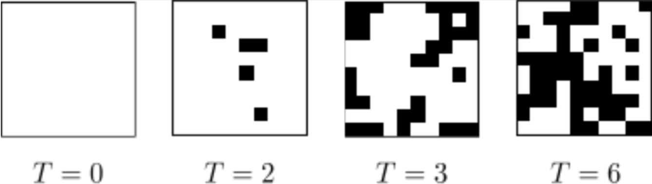
Figure 1: Examples of spin configurations at temperatures $T=0,2,3,6$

2.2 Unsupervised learning of the RBM

Our main motivation in the present paper is to study whether the RBM is related to the RG in statistical physics. In this section, we review the basic algorithm of the RBM [1, 10, 11, 12, 13, 14] which is trained by the configurations constructed by the MMC method of Sec. 2.1.

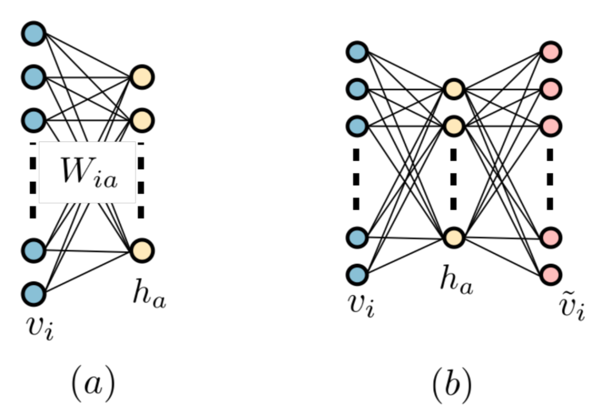
Figure 2: (a) Two-layer neural network of the RBM with a visible layer $\{v_{i}\}$ and a hidden layer $\{h_{a}\}$. These two layers are coupled but there are no intra-layer couplings. (b) The RBM generates reconstructed configurations from $\{v_{i}\}$ to $\{\tilde{v}_{i}\}$ through the hidden configuration $\{h_{a}\}$.

As explained in the Introduction, the RBM consists of two layers as shown in the left panel of Fig. 2. The initial configurations $\{\sigma_{x,y}\}$ of Ising model generated at various temperatures are input into the visible layer $\{v_{i}\}$. The number of neurons in the visible layer is fixed at $N_{v}=L^{2}=100$ ($i=1,\ldots,N_{v}$) to represent the spin configurations of Ising model. On the other hand, the hidden layer can take an arbitrary number of neurons, $N_{h}$. In the present paper, we consider 7 different sizes; $N_{h}=16,36,64,81,100,225$ and 400. Thus the $N_{h}$ spin variables in the hidden layer are given by $\{h_{a}\}$ for $a=1,\ldots,N_{h}$.

The RBM is a generative model of probability distributions based on Eq. (3). We first explain how we can train the RBM by optimizing the weights $W_{ia}$ and the biases $b_{i}^{(v)},b_{a}^{(h)}$. Our goal is to represent the given probability distribution $q_{0}(\{v_{i}\})$ in Eq. (6), as faithfully as possible, in terms of a model probability distribution defined by

$$p(\{v_{i}\})=\frac{1}{\cal Z}\sum_{\{h_{a}\}}e^{-\Phi(\{v_{i}\},\{h_{a}\})}.$$ (14)

The partition function ${\cal Z}=\sum_{\{v_{i},h_{a}\}}e^{-\Phi(\{v_{i}\},\{h_{a}\})}$ is difficult to evaluate, but summations over only one set of spin variables (e.g. over $\{v_{i}\}$) are easy to perform because of the absence of the intra-layer couplings. It also makes the conditional probabilities (4) and (5) to be rewritten as products of probability distributions of each spin variable;

$$p(\{h_{a}\}|\{v_{i}\})=\prod_{a}p(h_{a}|\{v_{i}\})=\prod_{a}\frac{1}{1+\exp\left[-2h_{a}\left(\sum_{i}W_{ia}v_{i}+b^{(h)}_{a}\right)\right]}$$ (15)

$$p(\{v_{i}\}|\{h_{a}\})=\prod_{i}p(v_{i}|\{h_{a}\})=\prod_{i}\frac{1}{1+\exp\left[-2{v}_{i}\left(\sum_{a}W_{ia}h_{a}+b^{(v)}_{i}\right)\right]}\,.$$ (16)

Then the expectation values of spin variables in the hidden (or visible) layer in the background of spin configurations in the other layer are calculated as

$$\langle h_{a}\rangle_{\{v_{i}\}}=\tanh\left(\sum_{i}W_{ia}v_{i}+b^{(h)}_{a}\right)$$ (17)

$$\langle v_{i}\rangle_{\{h_{a}\}}=\tanh\left(\sum_{a}W_{ia}h_{a}+b^{(v)}_{i}\right).$$ (18)

Now the task is to train the RBM so as to minimize the distance between two probability distributions of $q(\{v_{i}\})$ and $p(\{v_{i}\})$ by appropriately choosing the weights and the biases. The distance is called Kullback-Leibler (KL) divergence, or relative entropy, and given by

$$\text{KL}(q||p)=\sum_{\{v_{i}\}}q(\{v_{i}\})\log\frac{q(\{v_{i}\})}{p(\{v_{i}\})}=\text{const.}-\sum_{\{v_{i}\}}q(\{v_{i}\})\log p(\{v_{i}\})\,.$$ (19)

If two probabilities are equal, the KL divergence vanishes. Otherwise derivatives of KL$(q||p)$ with respect to the weight $W_{ia}$ and the biases $b_{i}^{(v)},b_{a}^{(h)}$ are given by

$$\frac{\partial\text{\,KL}(q||p)}{\partial W_{ia}} = \langle v_{i}h_{a}\rangle_{\text{data}}-\langle v_{i}h_{a}\rangle_{\text{model}}$$

$$\frac{\partial\text{\,KL}(q||p)}{\partial b_{i}^{(v)}} = \langle v_{i}\rangle_{\text{data}}-\langle v_{i}\rangle_{\text{model}}$$ (20)

$$\frac{\partial\text{\,KL}(q||p)}{\partial b_{a}^{(h)}} = \langle h_{a}\rangle_{\text{data}}-\langle h_{a}\rangle_{\text{model}}\,,$$

where averages are defined by

$$\langle A(\{v_{i}\})\rangle_{\text{data}}=\sum_{\{v_{i}\}}q(\{v_{i}\})A(\{v_{i}\})$$ (21)

$$\langle A(\{v_{i}\},\{h_{a}\})\rangle_{\text{model}}=\sum_{\{v_{i}\},\{h_{a}\}}p(\{v_{i}\},\{h_{a}\})A(\{v_{i}\},\{h_{a}\})\,,$$ (22)

and $h_{a}$ in $\langle\cdots\rangle_{\text{data}}$ is replaced by $\langle h_{a}\rangle_{\{v_{i}\}}$ of Eq. (17). In training the RBM, we change the weights and biases so that the KL divergence is reduced. Using the method of back propagation [22], we renew values of the weights and biases as

$$W~{} \to ~{}W_{\text{new}}=W+\delta W$$

$$b^{(v)}~{} \to ~{}b^{(v)}_{\text{new}}=b^{(v)}+\delta b^{(v)}$$

$$b^{(h)}~{} \to ~{}b^{(h)}_{\text{new}}=b^{(h)}+\delta b^{(h)}$$ (23)

where

$$\delta W_{ia} = \epsilon\left(\langle v_{i}h_{a}\rangle_{data}-\langle v_{i}h_{a}\rangle_{model}\right)$$

$$\delta b^{(v)}_{i} = \epsilon\left(\langle v_{i}\rangle_{data}-\langle v_{i}\rangle_{model}\right)$$

$$\delta b^{(h)}_{a} = \epsilon\left(\langle h_{a}\rangle_{data}-\langle h_{a}\rangle_{model}\right)\,.$$ (24)

Here $\epsilon$ denotes the learning rate, which we set to 0.1. The first terms $\langle\cdots\rangle_{{data}}$ are easy to calculate, but the second terms $\langle\cdots\rangle_{{model}}$ are difficult to evaluate since it requires the knowledge of the full partition function ${\cal Z}$.

To avoid this difficulty, we need to use the method of Gibbs sampling to approximately evaluate these expectation values $\langle\cdots\rangle_{{model}}$. Practically we employ a more simplified method, which is called the method of contrastive divergence (CD) [23, 24, 25]. The idea is very simple, and reminiscent of the mean field approximation in statistical physics. Given the input data of the visible spin configurations $\{v_{i}^{A(0)}=\sigma_{i}^{A}\}$, the expectation value of the hidden spin variable $h_{a}$ can be easily calculated as Eq. (17). We write the expectation value as

$$h_{a}^{A(1)}:=\langle h_{a}\rangle_{\{v_{i}^{A(0)}\}}=\tanh\left(\sum_{i}W_{ia}v_{i}^{A(0)}+b^{(h)}_{a}\right).$$ (25)

Then in this background of the hidden spin configurations, the expectation value of $v_{i}$ can be again easily calculated by using Eq. (18). We write it as

$$v_{i}^{A(1)}:=\langle v_{i}\rangle_{\{h_{a}^{A(1)}\}}=\tanh\left(\sum_{a}W_{ia}h_{a}^{A(1)}+b^{(v)}_{i}\right).$$ (26)

Then we obtain $h_{a}^{A(2)}=\langle h_{a}\rangle_{\{v_{i}^{A(1)}\}}$, and so on. We can iterate these procedure many times and replace the second terms in Eq. (20) by the expectation values generated by this method.

In doing the numerical simulations in the present paper, we adopt the simplest version of CD, called CD₁, which gives us the following approximate formulas:

$$\langle v_{i}\rangle_{data}=\frac{1}{N}\sum_{A}\sigma_{i}^{A},\quad\langle h_{a}\rangle_{data}=\frac{1}{N}\sum_{A}h_{a}^{A(1)},\quad\langle v_{i}h_{a}\rangle_{data}=\frac{1}{N}\sum_{A}\sigma_{i}^{A}h_{a}^{A(1)},$$ (27)

and

$$\langle v_{i}\rangle_{model}=\frac{1}{N}\sum_{A}v_{i}^{A(1)},\quad\langle h_{a}\rangle_{model}=\frac{1}{N}\sum_{A}h_{a}^{A(2)},\quad\langle v_{i}h_{a}\rangle_{model}=\frac{1}{N}\sum_{A}v_{i}^{A(1)}h_{a}^{A(2)}.$$ (28)

Here $\sigma_{i}^{A}$ denotes each spin configuration $\{\sigma_{x,y}\}$ generated by the method of Sec. 2.1. As input data to train the RBM, we generated 1000 spin configurations for each of 25 different temperatures $T=0,0.25,\ldots,6$. Then the index $A$ runs from $1$ to $N=25000$. In some cases, as we will see in Sec. 3.2, we use only a restricted set of configurations at high or low temperatures, then the index runs $A=1,\ldots,N=1000\times$(number of temperatures).

We repeat the renewal procedure (23) many times (5000 epochs), and obtain adjusted values of the weights and biases. In this way we train the RBM by using a set of configurations $\{v_{i}^{A(0)}=\sigma_{i}^{A}\}$, $(A=1,\ldots,N)$.

2.3 Generation of RBM flows

As discussed in the Introduction, once the RBM is trained and the weights and biases are fixed, the RBM generates a sequence of probability distributions (8). Then we translate the sequence into a flow of parameters (i.e., temperature). In generating the sequence, the initial set of configurations should be prepared separately in addition to the configurations that are used to train the RBM.

We can also generate a flow of parameters in a slightly different way. For a specific configuration $v_{i}=v_{i}^{(0)}$, we can define a sequence of configurations following Eqs. (25) and (26) as

$$\{v_{i}^{(0)}\}\rightarrow\{h_{a}^{(1)}\}\rightarrow\{v_{i}^{(1)}\}\rightarrow\{h_{a}^{(2)}\}\rightarrow\{v_{i}^{(2)}\}\rightarrow\cdots\,.$$ (29)

The right panel of Fig. 2 shows a generation of new configurations from $\{v_{i}\}$ to $\{\tilde{v}_{i}\}$ through $\{h_{a}\}$. Since each value of $v_{i}^{(n)}$ and $h_{a}^{(n)}$ (for $n>0$) is defined by an expectation value as in Eqs. (25) and (26), it does not take an integer $\pm 1$ but a fractional value between $\pm 1$. In order to get a flow of spin configurations, we need to replace these fractional values by $\pm 1$ with a probability $(1\pm\langle v_{i}^{(n)}\rangle)/2$ or $(1\pm\langle h_{a}^{(n)}\rangle)/2$. It turns out that the replacement is usually a good approximation since the expectation values are likely to take values close to $\pm 1$ owing to the property of the trained weights $|W_{ia}|\gg 1$. In this way, we obtain a flow of spin configurations

$$\{v_{i}^{(0)}\}\rightarrow\{v_{i}^{(1)}\}\rightarrow\{v_{i}^{(2)}\}\rightarrow\cdots\rightarrow\{v_{i}^{(n)}\}$$ (30)

starting from the initial configuration $\{v_{i}^{(0)}\}.$ The flow of configurations is transformed to a flow of temperature distributions by using the method explained in Sec. 2.4.

2.4 Temperature measurement by a supervised-learning NN

Next we design a neural network (NN) to measure temperature of spin configurations. The NN for the supervised learning has three layers with one hidden layer in the middle (See Fig. 3).

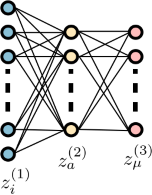
Figure 3: Three-layer neural network for supervised learning with an input layer $\{z_{i}^{(1)}\}$, a hidden layer $\{z_{a}^{(2)}\}$ and an output layer $\{z_{\mu}^{(3)}\}$.

The input layer $\{z^{(1)}_{i}\}$ consists of $L^{2}=100$ neurons in which we input spin configurations of Ising model. The output layer $\{z^{(3)}_{\mu}\}$ has $25$ neurons which correspond to 25 different temperatures that we want to measure. The number of neurons in the hidden layer $\{z^{(2)}_{a}\}$ is set to $64$. We train this three-layer NN by a set of spin configurations, each of which has a label of temperature. Thus this is the supervised learning. As input data to train the NN, we use the same $N=25000$ configurations which were used to train the RBM.

The training of the NN is carried out as follows. Denote the input data as

$$Z^{(1)}_{Ai}=\sigma_{i}^{A}$$ (31)

where $A=1,\ldots,N$, and $\sigma_{i}^{A}$ are the spin configurations $\{\sigma_{x,y}=\pm 1\}$ as in Sec. 2.2. The input data is transformed to $Z^{(2)}_{Aa}$ in the hidden layer by the following nonlinear transformation;

$$Z^{(2)}_{Aa}=f\left(\sum_{i=1}^{100}Z^{(1)}_{Ai}W^{(1)}_{ia}+b^{(1)}_{a}\right)=:f\left(U^{(1)}_{Aa}\right)$$ (32)

where $W^{(1)}_{ia}$ is an weight matrix and $b^{(1)}_{a}$ is a bias. The activation function $f(x)$ is chosen as $f(x)=\tanh(x)$. $Z^{(2)}_{Aa}$ is transformed to $Z^{(3)}_{A\mu}$ in the output layer, which corresponds to the label, namely temperature, of each configuration. The output $Z^{(3)}_{A\mu}$ is given by

$$Z^{(3)}_{A\mu}=g\left(\sum_{a=1}^{64}Z^{(2)}_{Aa}W^{(2)}_{a\mu}+b^{(2)}_{\mu}\right)=:g\left(U^{(2)}_{A\mu}\right)$$ (33)

where $W^{(2)}_{a\mu}$ and $b^{(2)}_{\mu}$ are another weight matrix and bias. The function $g(x)$ is the softmax function

$$g\left(U^{(2)}_{A\mu}\right)=\frac{\exp U^{(2)}_{A\mu}}{\sum_{\nu=1}^{25}\exp U^{(2)}_{A\nu}}\,,$$ (34)

so that $Z^{(3)}_{A\mu}$ can be regarded as a probability since $\sum_{\mu}Z^{(3)}_{A\mu}=1$ is satisfied for each configuration $A$. Thus the NN transforms an input spin configuration $Z^{(1)}_{Ai}$ to the probability $Z^{(3)}_{A\mu}$ of the configuration to take the $\mu$-th output value (i.e., temperature).

Each of the input configurations $Z^{(1)}_{Ai}$ is generated by the MMC method at temperature $T$. $T$ takes one of the 25 discrete values $T=\frac{1}{4}(\nu-1)$, ($\nu=1,\ldots,25$). If the A-th configuration is labelled by $\nu$, we want the NN to give an output $Z_{A\mu}^{(3)}$ as close as the following one-hot representation:

$$d_{A}^{(\nu)}=(0,\ldots,0,\check{1}^{(\nu)},0,\ldots,0)_{A}\,,$$ (35)

or its $\mu$-th component is given by $d_{A\mu}^{(\nu)}=\delta_{\mu\nu}$. It can be interpreted as a probability of the configuration $A$ to take the $\mu$-th output. Then the task of the supervised training is to minimize the cross entropy, which is equivalent to the KL divergence of the desired probability $d_{A\mu}^{(\nu)}$ and the output probability $Z^{(3)}_{A\mu}$. The loss function is thus given by the cross entropy,

$$E_{A}=\text{KL}(d_{A\mu}^{(\nu)}||Z^{(3)}_{A\mu})=-\sum_{\mu}d_{A\mu}^{(\nu)}\log Z^{(3)}_{A\mu}\,.$$ (36)

Then, using the method of back propagation, we renew values of the weights and biases from the lower to the upper stream;

$$W^{(\ell)}~{} \to ~{}W^{(\ell)}_{\text{new}}=W^{(\ell)}+\delta W^{(\ell)}$$

$$b^{(\ell)}~{} \to ~{}b^{(\ell)}_{\text{new}}=b^{(\ell)}+\delta b^{(\ell)}.$$ (37)

The variations of $\delta W^{(\ell)},\delta b^{(\ell)}$ at the lower stream are given by

$$\delta W^{(2)}_{a\mu} = -\frac{\epsilon}{N}\sum_{A}(Z^{(2)})^{T}_{aA}\Delta^{(3)}_{A\mu}$$

$$\delta b^{(2)}_{\mu} = -\frac{\epsilon}{N}\sum_{A}\Delta^{(3)}_{A\mu}$$ (38)

where $\Delta^{(3)}_{A\mu}=Z_{A\mu}^{(3)}-d_{A\mu}^{(\nu)}$. The learning rate $\epsilon$ is set to $0.1$. Then using these lower stream variations, we change the upper stream weights and biases as

$$\delta W^{(1)}_{ia} = -\frac{\epsilon}{N}\sum_{A}(Z^{(1)})^{T}_{iA}\Delta^{(2)}_{Aa}$$

$$\delta b^{(1)}_{a} = -\frac{\epsilon}{N}\sum_{A}\Delta^{(2)}_{Aa}$$ (39)

where

$$\Delta^{(2)}_{Aa} = \sum_{\mu}\Delta^{(3)}_{A\mu}(W^{(2)})^{T}_{\mu a}f^{\prime}\left(U^{(1)}_{Aa}\right).$$ (40)

We repeat this renewal procedure many times (7500 epochs) for the training of the NN to obtain suitably adjusted values of the weights and biases.

Finally we note how we measure temperature of a configuration. If the size of a configuration generated at temperature $T$ is large enough, say $L=10^{10^{100}}$, the trained NN will reproduce the temperature of the configuration quite faithfully. However our configurations are small sized with only $L=10$. Thus we instead need an ensemble of many spin configurations and measure a temperature distribution of the configurations. The supervised learning gives us this probability distribution of temperature.

3 Numerical results

In this section we present our numerical results for the flows generated by unsupervised RBM, and discuss a relation with the renormalization group flow of Ising model. Our main results of the RBM flows are written in Sec. 3.2.

3.1 Supervised learning for temperature measurement

Before discussing the unsupervised RBM, let us first see how we trained the NN to measure temperature.

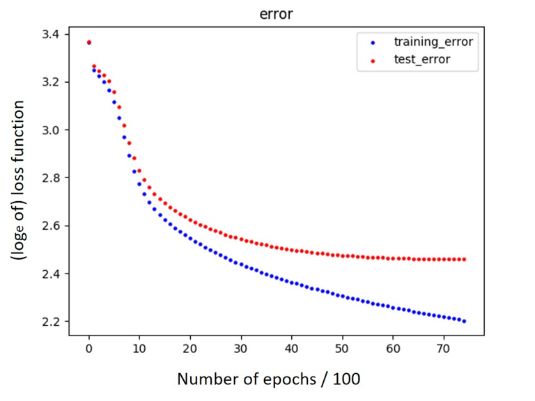
Figure 4: Training error and test error (up to 7500 epochs)

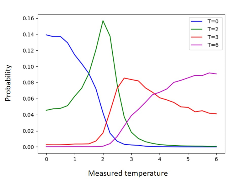
Figure 5: Probability distributions of measured temperatures for various sets of configurations generated at $T=0,2,3,6$ respectively. Temperature of the configurations can be distinguished by looking at the shapes of the distributions.

In Fig. 4, we plot behaviors of the loss function (36) as we iterate renewals of the weights and biases (37). The blue (lower) line shows the training error, namely values of the loss function (36) after iterations of training using 25000 configurations. It is continuously decreasing, even after 7500 epochs. On the other hand, the red (upper) line shows the test error, namely values of the loss function for additional 25000 configurations which are not used for the training. This is also decreasing at first, but after 6000 epochs it becomes almost constant. After 7500 epochs, in fact, it turns to increase. This means the machine becomes over-trained, therefore we stopped the learning at 7500 epochs.

In Fig. 5 we show probability distributions of temperature this NN measures. Here we use configurations at $T=0,2,3,6$ which are not used for the training. Though they are not sharply peaked at the temperatures where the configurations are generated, each of them has characteristic shape that is different temperature by temperature. Thus it is possible to distinguish the temperature of the input configurations by looking at the shape of the probability distribution, even if these configurations are not used for the training of the NN.

In the following, by using this NN, we measure temperature of configurations that are generated by the RBM flow.

3.2 Unsupervised RBM flows

Now we present the main results of the present paper, namely the flows generated by the unsupervised RBM. We sometimes call it the RBM flow. As discussed in the Introduction, if the RBM is similar to the the conventional RG in that it possesses a function of coarse-graining, the RBM flow must go away from the critical point $T_{c}=2.27$. In order to check it we construct three different types of unsupervised RBMs, which we call type V, type L, and type H respectively, using the method of Sec. 2.2. Each of them is trained by a different set of spin configurations generated at different set of temperatures. We then generate flows of temperature distributions by using these trained RBMs, following the methods of Secs. 2.3 and 2.4.

Type V RBM: Trained by configurations at $T=\{0,\ 0.25,0.5,\cdots,6\}$

First we construct type V RBM, which is trained by configurations at temperatures ranging widely from low to high, $T=0,0.25,\ldots,6$. The temperature range includes the temperature $T=2.25$ near $T_{c}$. After training is completed, this unsupervised RBM will have learned features of spin configurations at these temperatures.

Once the training is finished, we then generate a sequence of reconstructed configurations as in Eq. (30) using the methods in Sec. 2.3. For this, we prepare two different sets of initial configurations. One is a set of configurations at $T=0$, and another at $T=6$. These initial configurations are not used for the training of the RBM. Then by using the supervised NN in Sec. 3.1, we measure temperature and translate the flow of configurations to a flow of temperature distributions.

In Figs. 6 and 7, we plot temperature distributions of configurations that are generated by iterating the RBM reconstruction in Sec. 2.3. The “itr” in the legends means the numbers of iterations $n$ by the unsupervised RBM. Fig. 6 shows a flow of temperature distributions starting from spin configurations generated at $T=0$. Fig. 7 starts from $T=6.$ In all the figures, the black lines are the measured temperature distributions of the initial configurations. Colored lines show temperature distributions of the reconstructed configurations $\{v_{i}^{(n)}\}$ after various numbers of iterations. The left panels show the temperature distributions at small iterations (up to 10 in Fig. 6 and 50 in Fig. 7), while the right panels are at larger iterations up to 1000. These results indicate that the critical temperature $T_{c}$ is a stable fixed point of the flows in type V RBM. It is apparently different from a naive expectation that the RBM flow should show the same behavior as the RG flow. Indeed it is in the opposite direction. From whichever temperature $T=0$ or $T=6$ we start the RBM iteration, the peak of the temperature distributions approaches the critical point ($T=2.27$).

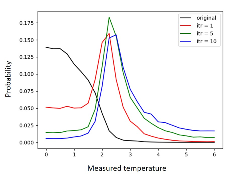
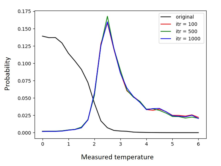
Figure 6: Temperature distributions after various numbers of iterations of type V RBM, which is trained by the configurations at $T=0,0.25,\ldots,6$. The original configurations are generated at $T=0$. After only several iterations, the temperature distribution is peaked around $T_{c}$, and stabilize there: $T_{c}$ is a stable fixed point of the flow.

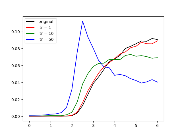
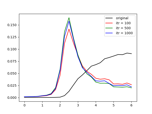
Figure 7: Temperature distributions after various numbers of iterations of the same RBM as Fig. 6. The original configurations are generated at $T=6$. After $\sim 50$ iterations, the distribution stabilizes at $T_{c}$.

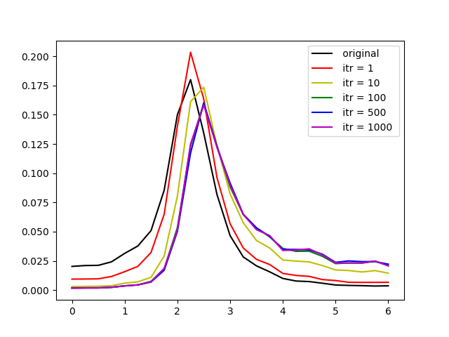
Figure 8: Temperature distributions after various numbers of iterations of the same RBM as Figs. 6 and 7. The original configurations are generated at $T=2.25$. The distribution is stable at around $T_{c}$.

In order to confirm the above behavior, we provide another set of configurations at $T=2.25$ as initial configurations, and generate the flow of temperature by the same trained RBM. The flow of temperature distributions is shown in Fig. 8. We can see that the temperature distribution of the reconstructed configurations remains near the critical point, and never flows away from there. If the process of the unsupervised RBM corresponds to coarse-graining of spin configurations, the temperature distributions of the reconstructed configurations must flow away from $T_{c}$. Though the direction of the flow is opposite to the RG flow, both flows have the same property in that the critical point $T=T_{c}$ plays an important role in controlling the flows.

So far, in obtaining the above results of Figs. 6, 7 and 8, we used an unsupervised RBM with 64 neurons in the hidden layer. We also trained other RBMs with different sizes of the hidden layer, but by the same set of spin configurations. When the size of the hidden layer is smaller than (or equal to) that of the visible layer $N_{v}=100$, namely $N_{h}=100,81,64,36$ or $16$, we find that the temperature distribution approaches the critical point. A difference is that for smaller $N_{h}$, the speed of the flow to approach $T_{c}$ becomes faster (i.e., the flow arrives at $T_{c}$ by smaller numbers of iterations).

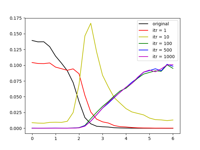
Figure 9: Temperature distribution after various numbers of iterations of type V RBM with 225 neurons in the hidden layer; i.e., $N_{h}>N_{v}$. The original configurations are generated at $T=0$. The distribution has a peak at $T=T_{c}$ after 10 iterations, but then moves towards $T=\infty$.

In contrast, when the RBM has more than 100 neurons in the hidden layer; $N_{h}>N_{v}$, we obtain different results. Fig. 9 shows the case of $N_{h}=225$ neurons. Until about ten iterations, the measured temperature distribution behaves similarly to the case of $N_{h}\leq 100$, i.e., it approaches the critical temperature. However, afterward it passes the critical point and flows away to higher temperature. In the case of 400 neurons, it moves towards high temperature at faster speed. This behavior suggests that, if the hidden layer has more than a necessary size, the NN tends to learn a lot of noisy fluctuations. Since configurations at higher temperatures are noise-like, the flow should go away to high temperature. We come back to this conjecture in later sections.

Type H/L RBM: Trained by configs at Higher/Lower temperatures

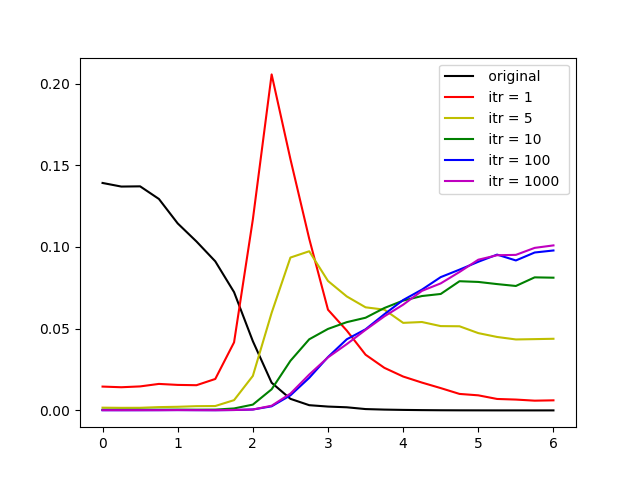
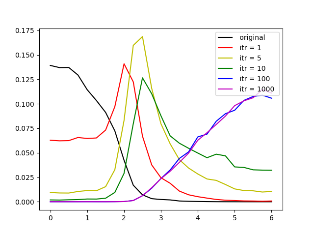
Figure 10: Flow of temperature distributions starting from $T=0$ in type H RBM. Type H RBM is trained by configurations at only $T=4,4.25,\ldots,6$. The NN has $N_{h}=64$ neurons (left) and $N_{h}=225$ neurons (right) respectively in the hidden layer. The speed of the flow is slower for the larger sized hidden layer.

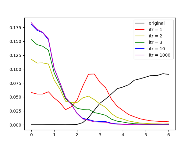
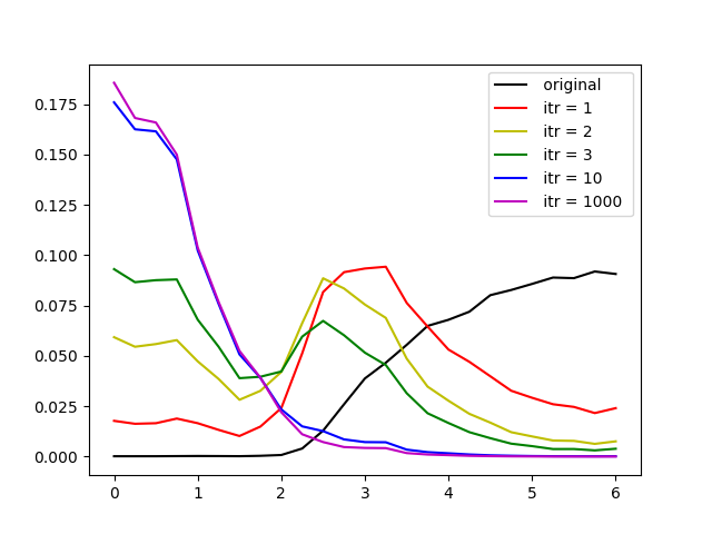
Figure 11: Flow of temperature distributions starting from $T=6$ in type L RBM. Type L RBM is trained by configurations at only $T=0$. $N_{h}=64$ (left) and $N_{h}=225$ (right).

Next we construct another type of RBM, which is trained by configurations at higher temperatures $T=4,4.25,\ldots,6$ than $T_{c}\sim 2.25.$ We call it type H RBM. The results of the flows of temperature distributions in type H RBM are drawn in Fig. 10. In this case, the measured temperature passes the critical point and goes away towards higher temperature. The behavior is understandable since the RBM must have learned only the features at higher temperatures. We also find that, if the number of neurons in the hidden layer is increased, the flow moves more slowly.

Finally, we construct type L RBM, which is trained by configurations only at the lowest temperature $T=0$. Fig. 11 shows the numerical results of flows in the type L RBM. Similarly to the type H RBM, the measured temperature passes the critical point, but flows towards lower temperature instead of higher temperature. It is, of course, as expected because the type L RBM must have learned the features of spin configurations at $T=0$. In the type L RBM, as far as we have studied, the flow never goes back to higher temperature even for large $N_{h}$. It will be because the $T=0$ configurations used for training do not at all contain noisy fluctuations specific to high temperatures. This also suggests that the RBM does not learn features that are not contained in the configurations used for trainings.

Summaries and Conjectures

Here we first summarize the numerical results:

For the type V RBM,

• When $N_{h}\leq 100=N_{v}$, the measured temperature $T$ approaches $T_{c}$ (Figs. 6, 7 and 8).

• However, for $N_{h}>100=N_{v}$, the flow eventually goes away towards $T=\infty$ (Fig. 9).

• Speed of flow is slower for a larger $N_{h}$.

For the type H/L RBM,

• The temperature $T$ flows towards $T=\infty/T=0$ respectively (Figs. 10 and 11).

• Speed of flow is slower for a larger $N_{h}$.

Here $N_{h}$ and $N_{v}$ are numbers of hidden and visible neurons in the RBM. These behaviors are reflections of the properties of the weights and biases that the unsupervised RBMs have learned in the process of training.

Understanding the above behaviors is equivalent to answering what the unsupervised RBMs have learned in the process of trainings. The most important question will be why the temperature approaches $T_{c}$ in the type V RBM with $N_{h}\leq N_{v}$, instead of, e.g., broadening over the whole regions of temperature from $T=0$ to $T=6$. Note that we did not teach the NN neither about the critical temperature nor the presence of phase transition. We just have trained the NN by configurations at various temperatures, from $T=0$ to $T=6$. Nevertheless the numerical simulations show that the temperature distributions are peaked at $T_{c}$ after some iterations of the RBM reconstruction. Thus we are forced to conclude that the RBM has automatically learned features specific to the critical temperature $T_{c}$.

An important feature at $T_{c}$ is the scale invariance. We have generated spin configurations at various temperatures by the Monte Carlo method, and each configuration has typical fluctuations specific to each temperature. At very high temperature, fluctuations are almost random at each lattice site and there are no correlations between spins at distant positions. At lower temperature, they become correlated: the correlation length becomes larger as $T\rightarrow T_{c}$ and diverges at $T_{c}$. On the other hand, at $T\ll T_{c}$, spins are clustered and in each domain all spins take $\sigma_{x,y}=+1$ or $\sigma_{x,y}=-1$. At low temperature configurations have only big clusters, and as temperature increases small-sized clusters appear. At $T_{c}$, spin configurations become to have clusters of various sizes in a scale-invariant way.

Now let us come back to the question why the type V RBM generates a flow approaching $T_{c}$ and does not randomize to broaden the temperature distribution over the whole regions. We have trained the type V RBM by using configurations at various temperatures with different sized clusters, and in the process the machine must have simultaneously acquired features at various temperatures. Consequently the process of the RBM reconstruction adds various features that the machine has learned to a reconstructed configuration. If only a single feature at a specific temperature was added to the reconstructed configuration, the distribution would become to have a peak at this temperature. But it cannot happen because various features of different temperatures will be added to a single configuration by iterations of reconstruction processes. Then one may ask if there is a configuration that is stable under additions of features at various different $T$.

Our first conjecture about this question is that a set of configurations at $T_{c}$ is a stabilizer (and even more an attractor) of the type V RBM with $N_{h}\leq N_{v}$. It must be due to the scale invariant properties of the configurations at $T_{c}$. Namely since these configurations are scale invariant, they have all the features of various temperatures simultaneously, and consequently they can be the stabilizer of this RBM. This sounds plausible since the scale invariance means that the configurations have various different characteristic length scales. However, we notice that this doesn’t mean that the RBM has forgotten the features of configurations away from the critical point. Rather it means that the RBM has learned features of all temperatures simultaneously. This doesn’t mean either that the configurations at $T=T_{c}$ have especially affected strong influence on the machine in the process of training. It can be confirmed as follows. Suppose we have trained a RBM by configurations at temperatures excluding $T=T_{c}$, namely train by configurations at all temperatures except $T=2.25$ and $2.5$. We found in the numerical simulations that the RBM generates a flow towards the critical point though we did not provide configurations at $T=T_{c}$. Therefore we can say that the type V RBM has learned the features at all the temperatures and that configurations at $T_{c}$ are special because they contain all the features of various temperatures in the configurations.

Our second conjecture, which is related to the behavior of the type V RBM with $N_{h}>N_{v}$, is that RBMs with unnecessary large sized hidden layer tend to learn lots of irrelevant features. In the present case, they are noisy fluctuations of configurations at high temperatures. High temperature configurations have only short distance correlations, whose behavior is similar to the typical behavior of noise. The conjecture will be partially supported by the similarity of the RBM flows between the type V RBM with $N_{h}>N_{v}$ and the type H RBM. Namely both RBM flows converge on $T=\infty$. The similarity indicates that the NN with a larger number of $N_{h}$ may have learned too much noise-like features of configurations at higher temperatures. The above considerations will teach us that the moderate size of the hidden layer, $N_{h}<N_{v}$, is the most efficient to properly extract the features.

4 Analysis of the weight matrix

In the previous section, we showed our numerical results for the flows generated by unsupervised RBMs, and proposed two conjectures. One is that the scale invariant $T=T_{c}$ configurations are stabilizers of the type V RBM flow. Another conjecture is that the RBM with an unnecessary large sized hidden layer $N_{h}>N_{v}$ tends to learn too much irrelevant noises. In this section, to further understand the theoretical basis of feature extractions and to give supporting evidences for our conjectures, we analyze various properties of the weight matrices and biases of the trained RBMs. Particularly, we study properties of $WW^{T}$ by looking at spin correlations in Sec. 4.2, magnetization in Sec. 4.3, and eigenvalue spectrum in Sec. 4.4.

4.1 Why $WW^{T}$ is important

All the information that the machine has learned is contained in the weights $W_{ia}$ and the biases $b_{i}^{(v)},b_{a}^{(h)}$. Since the biases have typically smaller values than the weights (at least in the present situations), we will concentrate on the weight matrix $W_{ia}$ ($i=1,\ldots,N_{v}=L^{2}$; $a=1,\ldots,N_{h}$) in the following.

Let us first note that the weight matrix $W_{ia}$ transforms as

$$W_{ia}~{}\rightarrow~{}\tilde{W}_{ia}=\sum_{j,b}U_{ij}W_{ib}(V^{T})_{ba}$$ (41)

under transformations of exchanging the basis of neurons in the visible layer ($U_{ij}$) and in the hidden layer ($V_{ab}$). Since the choice of basis in the hidden layer is arbitrary, relevant information in the visible layer is stored in a combination of $W_{ia}$ that is invariant under transformations of $V_{ab}$. The simplest combination is a product,

$$(WW^{T})_{ij}=\sum_{a}W_{ia}W_{aj}\,.$$ (42)

It is an $N_{v}\times N_{v}=100\times 100$ matrix, and independent of the size of $N_{h}$. But its property depends on $N_{h}$ because the rank of $WW^{T}$ must be always smaller than $\min(N_{v},N_{h})$. Thus, if $N_{h}<N_{v}$, the weight matrix is strongly constrained; e.g. a unit matrix $WW^{T}=1$ is not allowed.

This simplest product (42) plays an important role in the dynamics of the flow generated by the RBM. It can be shown as follows. If the biases are ignored, the conditional probability (15) and the expectation value (17) for $h_{a}$ in the background of $v_{i}$ become

$$p(\{h_{a}\}|\{v_{i}\})=\frac{e^{\sum_{i}v_{i}W_{ia}h_{a}}}{2\cosh\left(\sum_{i}v_{i}W_{ia}\right)}\,,\qquad\langle h_{a}\rangle=\tanh\left(\sum_{i}v_{i}W_{ia}\right)\,.$$ (43)

In $p(\{h_{a}\}|\{v_{i}\})$, a combination $\sum_{i}v_{i}W_{ia}=:B_{a}$ can be regarded as an external magnetic field for $h_{a}$. Thus these two variables, $B_{a}$ and $h_{a}$, tend to correlate with each other. Namely, the probability $p(\{h_{a}\}|\{v_{i}\})$ becomes larger when they have the same sign. Moreover, for $|B_{a}|<1$, $\langle h_{a}\rangle$ is approximated by $B_{a}$ and we can roughly identify these two variables,

$$\langle h_{a}\rangle\sim B_{a}:=\sum_{i}v_{i}W_{ia}\,.$$ (44)

It is usually not a good approximation since weights can have larger values, but let us assume this for the moment. For a large value of $|B_{a}|$, $\langle h_{a}\rangle$ is saturated at $\langle h_{a}\rangle=B_{a}/|B_{a}|$.

Suppose that the input configuration is given by $\{v_{i}^{(0)}\}=\{\sigma_{i}^{A}\}$. If Eq. (44) is employed, we have $h_{a}^{(1)}=B_{a}^{(0)}=\sum_{i}v_{i}^{(0)}W_{ia}.$ Then the conditional probability (16) in the background of $h_{a}^{(1)}$ with $b_{a}^{(h)}=0$,

$$p(\{v_{i}\}|\{h_{a}^{(1)}\})=\prod_{i}\frac{e^{\sum_{a}v_{i}W_{ia}h_{a}^{(1)}}}{2\cosh\left(\sum_{a}W_{ia}h_{a}^{(1)}\right)}$$ (45)

can be approximated as

$$p(\{v_{i}\}|\{h_{a}^{(1)}\})\sim\prod_{i}\frac{e^{\sum_{a}v_{i}W_{ia}\sum_{j}W_{ja}v_{j}^{(0)}}}{2\cosh\left(\sum_{a}W_{ia}\sum_{j}W_{ja}v_{j}^{(0)}\right)}=\prod_{i}\frac{e^{\sum_{j}v_{i}(WW^{T})_{ij}v_{j}^{(0)}}}{2\cosh\left(\sum_{j}(WW^{T})_{ij}v_{j}^{(0)}\right)}\,.$$ (46)

The RBM learns the input data $\{v_{j}^{(0)}\}$ so that the probability distribution $p$ reproduces the probability distribution of the initial data, $q(\{v_{i}\})=\frac{1}{N}\sum_{A}\delta(v_{i}-\sigma_{i}^{A})$. Therefore, training of the RBM will be performed so as to enhance the value $\sum_{A,i,j}\sigma_{i}^{A(0)}(WW^{T})_{ij}\sigma_{j}^{A(0)}$. This means that $W$ is chosen so that $(WW^{T})_{ij}$ will reflect the spin correlations of the input configurations $\{\sigma_{i}^{A}\}$ at site $i$ and $j$.

In this simplified discussion, learning of the RBM is performed through the combination $WW^{T}$. Of course, we neglected the nonlinear property of the neural network and the above statement cannot be justified as it is. Nevertheless, we will find below that the analysis of $WW^{T}$ is quite useful to understand how the RBM works.

4.2 Spin correlations in $WW^{T}$

In Fig. 12, we plot values of matrix elements of the $100\times 100$ matrix $WW^{T}$. These three figures correspond to the RBMs with different sizes of $N_{h}$. We can see that they have large values in the diagonal and near diagonal elements. Note that the spin variables in the visible layer, $\sigma_{x,y}$ with $x,y=1,\ldots,L=10$, are lined up as $(\sigma_{1,1},\sigma_{1,2},\ldots,\sigma_{1,L},\sigma_{2,1},\ldots,\sigma_{2,L},\sigma_{3,1},\ldots,\sigma_{L,L})$, and named $(\sigma_{1},\sigma_{2},\ldots,\sigma_{N})$. Hence lattice points $i$ and $j$ of $\sigma_{i}$ ($i=1,\ldots,L^{2}$) are adjacent to each other when $j=i\pm 1$ and $j=i\pm L$. In the following, we mostly discuss the type V RBM unless otherwise stated.

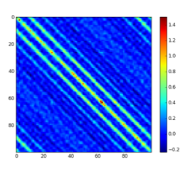
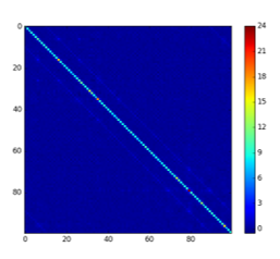
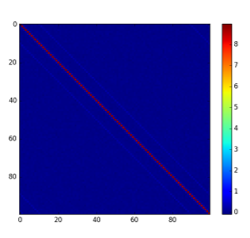
Figure 12: Elements of $WW^{T}$ when the hidden layer has 16 (left), 100 (center), 400 (right) neurons.

As discussed above, the product of weight matrices $WW^{T}$ must reflect correlations between spin variables of the input configurations used for the training of the RBM. The most strong correlation in $v_{i}^{(0)}(WW^{T})_{ij}v_{j}^{(0)}$ is of course the diagonal component, $i=j$. Thus we expect that the matrix $WW^{T}$ will have large diagonal components. Indeed, such behavior can be seen in Fig. 12. In particular, for $N_{h}=400>N_{v}=100$ (the rightmost figure), $WW^{T}$ is clearly close to a diagonal matrix. It is almost true for the case of $N_{h}=100=N_{v}$ (the middle figure). However, for $N_{h}=16<N_{v}=100$ (the leftmost figure), it is different from a unit matrix and off-diagonal components of $(WW^{T})_{ij}$ also have large values, in particular, at $j=i+1$ and $j=i+2$. This behavior must be a reflection of the spin correlations of the input configurations . It is also a reflection of the fact that the rank of $WW^{T}$ is smaller than $N_{h}$ and $WW^{T}$ cannot be a unit matrix if $N_{h}<N_{v}$. Thus even though only less information can be stored in the weight matrix for a smaller number of hidden neurons, the relevant information of the spin correlations is well encoded in the weight matrix of the RBM with $N_{h}<N_{v}$ compared with the RBM with larger $N_{h}$. Then we wonder why such relevant information is lost in the RBM with $N_{h}>N_{v}$. This question might be related to our second conjecture proposed at the end of Sec. 3.2 that the RBM with very large $N_{h}$ will learn too much irrelevant information, namely noises of the input configurations. It is interesting and a bit surprising that the RBM with fewer hidden neurons seems to learn more efficiently the relevant information of the spin correlations.

In order to further confirm the relation between the correlations in the combination of the weight matrix $WW^{T}$ and the spin correlations of the input configurations, we will study structures of the weight matrices of other types of RBMs. In Fig. 13, we plot behaviors of the off-diagonal components of $WW^{T}$ for various RBMs. Each RBM is trained by configurations at a single temperature $T=0$ (type L), $T=2$, $T=3$ and $T=6$ respectively. The size of the hidden layer is set to $N_{h}=16$. For comparison, we also plot the behavior of the off-diagonal components for the type V RBM.

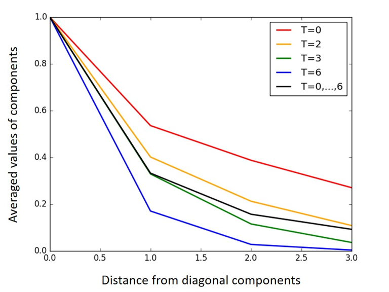
Figure 13: Averaged values of the off-diagonal components of $WW^{T}$ (normalized by the diagonal components). Each colored line corresponds to the RBM that has learned configurations at a single temperature $T=0,2,3,6$ respectively. The black line (the most middle line) is the behavior of the type V RBM that has learned all the temperatures $T=0,\ldots,6$.

Fig. 13 shows that the correlation of $WW^{T}$ decays more rapidly at higher temperature, which is consistent with the expected behavior of spin correlations. Therefore, the RBM seems to learn correctly about the correlation length, or the size of clusters, which becomes smaller at higher temperature. Furthermore, we find that, for the type V RBM that has learned all temperatures $T=0,\ldots,6$, the off-diagonal elements decrease with the decay rate between the $T=2$ case and the $T=3$ case. This indicates that the type V RBM has acquired similar features to those of the configurations around $T_{c}=2.27$. It is consistent with the numerical results of Figs. 6, 7 and 8, and gives another circumstantial evidence supporting for the first conjecture in Sec. 3.2.

4.3 Magnetization and singular value decomposition (SVD)

Information of the weight matrix $W$ can be inferred by using the method of the singular value decomposition (See, e.g., [26, 27]). Suppose that the matrix $WW^{T}$ has eigenvalues $\lambda_{a}$ ($a=1,\ldots,N_{v})$ with corresponding eigenvectors $u_{a}$;

$$WW^{T}u_{a}=\lambda_{a}u_{a}\,.$$ (47)

Decomposing an input configuration vector $v^{(0)}$ in terms of the eigenvectors $u_{a}$ as $v^{(0)}=\sum_{a}c_{a}u_{a}$ with a normalization condition $\sum_{a}(c_{a})^{2}=1$, we can rewrite $v^{(0)T}WW^{T}v^{(0)}$ as

$$v^{(0)T}WW^{T}v^{(0)}=\sum_{a}c_{a}^{2}\lambda_{a}\,.$$ (48)

Thus if a vector $v^{(0)}$ contains more components with larger eigenvalues of $WW^{T}$, the quantity $v^{(0)T}WW^{T}v^{(0)}$ becomes larger.

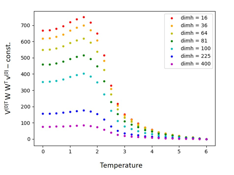
Figure 14: Averaged values of $v^{(0)T}WW^{T}v^{(0)}$ over the 1000 input configurations at each temperature. Different colors correspond to type V RBMs with different number of hidden neurons $N_{h}$. In this figure, the values at $T=6$ are subtracted for comparison between different RBMs.

Fig. 14 shows averaged values of $v^{(0)T}WW^{T}v^{(0)}$ over the 1000 configurations $\{v^{(0)}\}$ at each temperature. For comparison between different RBMs, we subtracted the values at $T=6$. The figure shows a big change near the critical point, which is reminiscent of the magnetization of Ising model. Since $v^{(0)T}WW^{T}v^{(0)}$ should contain more information than the magnetization itself, the behavior cannot be exactly the same. But it is quite intriguing that Fig. 14 shows similar behavior to the magnetization. It might be because the quantity contains much information about the lower temperature after subtraction of the values at higher temperature.

In order to see the properties of $v^{(0)T}WW^{T}v^{(0)}$ more than the magnetization in Fig. 14, we plot the same quantities but without subtracting the values at $T=6$. Fig. 15 shows two cases for $N_{h}=64$ and $N_{h}=225.$

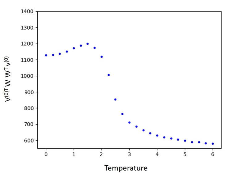
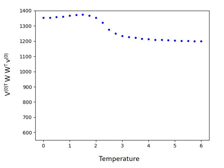
Figure 15: Averaged values of $v^{(0)T}WW^{T}v^{(0)}$ over the 1000 configurations $\{v^{(0)}\}$ at each temperature. The left and right figure shows the quantities in the type V RBM with $N_{h}=64$ and $N_{h}=225$ respectively.

These figures show that, at high temperature, the RBM with large $N_{h}$ in the right panel has larger components of the principal eigenvectors compared to the RBM with small $N_{h}$ in the left panel. The difference must have caused the different behaviors in the RBM flows shown in Fig. 6 ($N_{h}=64)$ and Fig. 9 ($N_{h}=225$). Namely the former RBM flow approaches the critical temperature $T_{c}$, while the latter eventually goes towards higher temperature. The difference of two figures in Fig. 14 indicate that the RBM with larger $N_{h}$ seems to have learned more characteristic features at high temperatures than the RBM with fewer $N_{h}$. Then, does the RBM with small $N_{h}$ fail to learn the features of high temperatures? Which RBM is more adequate for feature extractions? Although it is difficult to answer which is more adequate without specifying what we want the machine to learn, we believe that the RBM with $N_{h}<N_{v}$ properly learns all the features of various temperatures while the RBM with $N_{h}>N_{v}$ has learned too much irrelevant features of high temperature. This is nothing but the second conjecture in Sec. 3.2, and supported by the behaviors of correlations in $WW^{T}$ discussed in Sec. 4.2.

4.4 Eigenvalue spectrum and information stored in $W$

Finally we study the eigenvalue spectrum $\lambda_{a}$ of the matrix $WW^{T}$. Figs. 16 and 17 show the eigenvalues in the descending order.

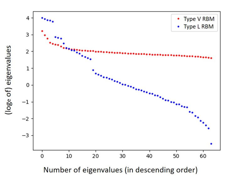
Figure 16: Eigenvalues of $WW^{T}$ for type V RBM (red, a smooth line) and type L RBM (blue, a steplike line). Both RBMs have 64 neurons in the hidden layer.

In Fig. 16, the red dots (a smooth line) show the eigenvalues of the type V RBM trained by configurations at all the temperatures ($T=0,0.25,\ldots,6$), while the blue dots (a steplike line) are the eigenvalues of the type L RBM (only $T=0$).

These are obviously different. For the type L RBM, only several eigenvalues are especially large, and the rest are apparently smaller. On the other hand, for the type V RBM, the eigenvalues decrease gradually and there are no jumps or big distinctions between larger and smaller eigenvalues. The behavior indicates that, in the type L RBM, the weight matrix holds only small relevant information and only a small number of neurons is sufficient in the hidden layer. In the type V RBM, however, since it is trained by configurations at various different temperatures, all the eigenvectors are equally utilized to represent relevant features of spin configurations at various temperatures. Namely, in order to learn features of a wide range of temperatures, larger number of neurons in the hidden layer are necessary. Using such larger degrees of freedom, the weight matrix has learned configurations with various characteristic scales at various temperatures so that the RBM can grasp rich properties of these configurations.

The difference of the eigenvalues between type V and type L is also phrased that type V has a scale invariant eigenvalue spectrum. In contrast, the eigenvalues of the type L RBM are separated into distinct regions in which the corresponding eigenvalues might represent features with different scales. It might be related to our previous numerical results, shown in Figs. 6, 7 and 8, that type V RBM generates a flow toward the critical point where the configurations have scale invariance.

Finally in Fig. 17 we show differences in eigenvalue spectrum between RBMs with different numbers of hidden neurons $N_{h}$.

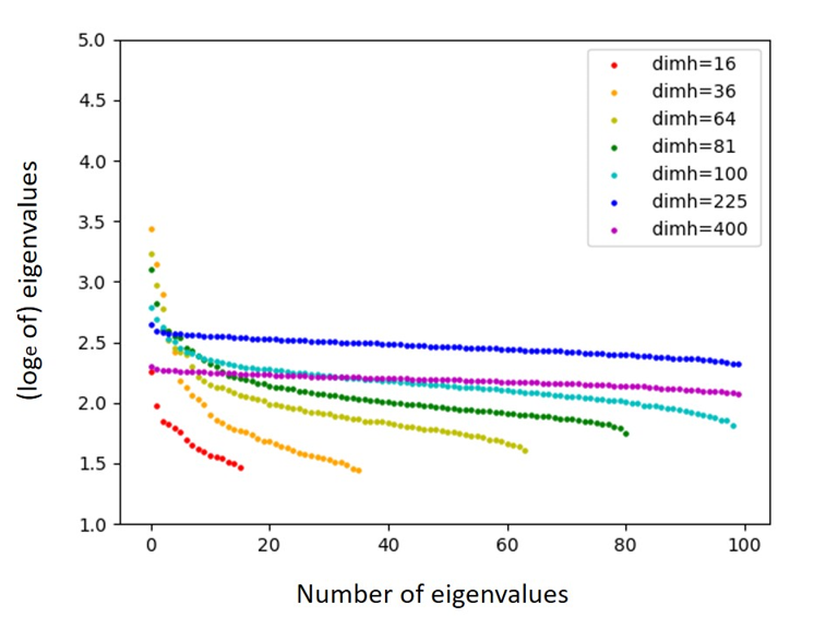
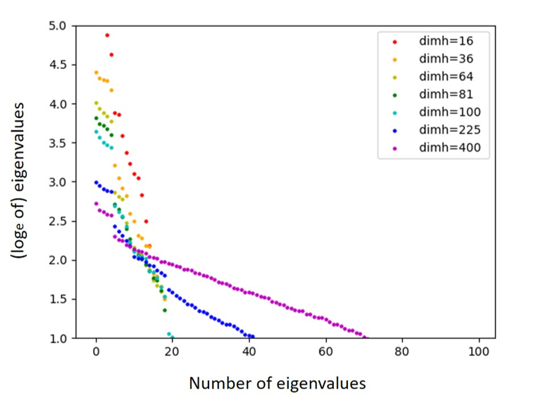
Figure 17: Eigenvalues of $WW^{T}$ for type V RBM (left) and type L RBM (right). The legend shows the number of hidden neurons $N_{h}$.

As shown in the left panel of Fig. 17, in the type V RBM with $N_{h}>N_{v}=100$, most eigenvalues have similar values. In contrast, for a smaller $N_{h}$, large and small eigenvalues are very different and the spectrum has a hierarchical structure. The type L RBM shows similar behaviors as shown in the right panel of Fig. 17. It might indicate that the RBM with larger $N_{h}$ ($>N_{v}$) has learned too much details of the input configurations and the most relevant features are weakened. In other words, it has learned too much irrelevant features which are especially specific to configurations at higher temperature. It may explain our numerical results shown in Fig. 9, which is apparently different from Fig. 6, that the flow first approaches the critical point but passes there and eventually goes away to higher temperature. This view is consistent with the discussion at the end of Sec. 4.3 and supports the second conjecture in Sec. 3.2.

To summarize, we find that the type V RBM with smaller $N_{h}$ than $N_{v}$ can adequately learn configurations at wide range of temperatures, without learning too much features at higher temperature. All the neurons in the hidden layer are efficiently used to represent features of various temperatures in a scale invariant way as seen in the eigenvalue spectrum. As a result, after many iterations of the RBM reconstruction, initial configurations are transformed into the configurations around the critical temperature $T_{c}$. Thus the RBM flow has similarity with the RG flow, but the RBM flow is in the opposite direction to the conventional RG flow and a naive analogy does not hold.

5 Discussions

In this paper, in order to see what the restricted Boltzmann machine (RBM) learns in the process of training, we investigated flow of configurations generated by the weight matrices of the RBM. In particular, we studied the Ising model and found that, if the RBM is trained by spin configurations at various different temperatures (we call it type V RBM), the temperature of an initial configuration flows towards the critical point $T=T_{c}$ where the system becomes scale invariant. The result suggests that the configurations at $T=T_{c}$ are attractors of the RBM flow. In order to understand the numerical results of the RBM flows and to find a clue of what the machine has learned, we explored properties of the weight matrix $W_{ia}$ , especially those of the product $WW^{T}$, by looking at the eigenvalue spectrum.

There are still many unsolved issues left for future investigations. If we admit that an eigenvector represents a “feature” that the RBM has learned, the magnitude of the corresponding eigenvalue is an indicator of how much influence the feature affects, and reminiscent of the critical exponents of relevant operators in the renormalization group (RG). It will be interesting to pursue this analogy further and to extract more information from the eigenvalue spectrum and to connect with the behaviors of the RBM flow. The RBM flow gives important clues of what the machine has learned. If an RBM is trained by configurations at a single specific temperature, it generates a flow toward that temperature. This confirms a hypothesis that the unsupervised RBM indeed extracted relevant features of the configurations and the flow is consequently attracted to the configurations with these relevant features. The RBM flow is a stochastic process with a random noise, and should be described by the Langevin (or Fokker Planck) equation, whose drift term is given by the relevant features. We want to come back to this problem in future investigations.

In the present paper, we picked up the Ising model, the simplest statistical model of the second order phase transition and found that the critical point is an attractor of the RBM flow. Then we wonder what happens in the case of the first order phase transition. A simple example is the Blume-Capel model on a two dimensional lattice. The Hamiltonian is given by $\beta H=-J\sum_{ij}s_{i}s_{j}+\Delta\sum_{i}s_{i}^{2}$ where $s_{i}=\pm 1,0$ is a spin at site $i$. The model undergoes the first order phase transition that separates the parameter space $(J,\Delta)$, and the second order phase transition at the tricritical point $(J_{c},\Delta_{c})$. If we train an RBM by configurations at various different parameters (such as the type V RBM of the Ising model), the flow of parameters will be attracted to the tricritical point. On the other hand, if we use only a restricted set of configurations for training, e.g. various $J$ with a fixed $\Delta(<\Delta_{c})$, where is the RBM flow attracted? It is not certain whether it is attracted to the phase boundary of the first order phase transition or to the tricritical point. It is under investigations and we want to report the numerical results in future publications.

Finally we would like to comment on a possible relation between structures of RBM flows and how we recognize the world around us. Our finding is that there is an attractor of the RBM flow which characterizes the relevant feature that machine has learned before. We human beings also meet similar phenomena, namely we can recognize more easily and comfortably what we have already learned many times than what we first experience. Also what we think beautiful is not what we experience first but usually a combination of what we have already experienced before. A good example will be looking at abstract paintings or tasting bitter coffee. It suggests that attractors are constructed in the process of learnings and we would feel comfortable when input data are close to the attractors of the neural network in our brain. For verification of the conjecture, it must be amusing to train a RBM by inputting varieties of human faces and generate the RBM flow of a human face to see if there is an attractor face. The attractor might provide a standard for beauty. In this way, we can guess that attractors of the RBM flows in the NN of our brain may control our value judgments.

Acknowledgments

We would like to thank participants of I-URIC frontier colloquium 2017, especially Shunichi Amari, Taro Toyoizumi and Shinsuke Koyama for fruitful discussions. We also thank Masato Taki for his intensive lectures on machine learning at KEK. This work of S.I. and S.S. is supported in part by Grants-in-Aid for Scientific Research (No. 16K05329 and No. 16K17711, respectively) from the Japan Society for the Promotion of Science (JSPS).

References

- [1] G. E. Hinton and R. R. Salakhutdinov, “Reducing the dimensionality of data with neural networks,” Science 313 (2006) 504.
- [2] C. Bény, “Deep learning and the renormalization group,” arXiv:1301.3124 [quant-ph].
- [3] S. Saremi and T. J. Sejnowski, “Hierarchical model of natural images and the origin of scale invariance,” Proceedings of the National Academy of Sciences 110 (2013) 3071.
- [4] P. Mehta and D. J. Schwab, “An exact mapping between the Variational Renormalization Group and Deep Learning,” arXiv:1410.3831 [stat.ML].
- [5] A. Paul and S. Venkatasubramanian, “Why does Deep Learning work? - A perspective from Group Theory,” arXiv:1412.6621 [cs.LG].
- [6] H. W. Lin, M. Tegmark and D. Rolnick, “Why Does Deep and Cheap Learning Work So Well?,” J. Stat. Phys. 168 (2017) 1223-1247 [arXiv:1608.08225 [cond-mat.dis-nn]].
- [7] M. Sato, “Renormalization Group Transformation for Hamiltonian Dynamical Systems in Biological Networks,” arXiv:1609.02981 [q-bio.OT].
- [8] K.-I. Aoki and T. Kobayashi, “Restricted Boltzmann machines for the long range Ising models,” Mod. Phys. Lett. B 30 (2016) 1650401 [arXiv:1701.00246 [cond-mat.stat-mech]].
- [9] M. Koch-Janusz and Z. Ringel, “Mutual Information, Neural Networks and the Renormalization Group,” arXiv:1704.06279 [cond-mat.dis-nn].
- [10] R. Salakhutdinov, A. Mnih and G. Hinton, “Restricted Boltzmann machines for collaborative filtering,” Proceedings of the 24th international conference on Machine learning (ACM, 2007) pp. 791-798.
- [11] H. Larochelle and Y. Bengio, “Classification using discriminative restricted Boltzmann machines,” Proceedings of the 25th international conference on Machine learning (ACM, 2008) pp. 536-543.
- [12] G. Hinton, “A practical guide to training restricted Boltzmann machines,” Momentum 9 (2010) 926.
- [13] G. E. Hinton, “A principal guide to training restricted Boltzmann machines,” Neural networks: Tricks of the Trade, Springer (2012) pp. 599-619.
- [14] D. S. P. Salazar, “Nonequilibrium Thermodynamics of Restricted Boltzmann Machines,” Phys. Rev. E 96 (2017) 022131 [arXiv:1704.08724 [cond-mat.stat-mech]].
- [15] K. G. Wilson, “Renormalization group and critical phenomena. 1. Renormalization group and the Kadanoff scaling picture,” Phys. Rev. B 4 (1971) 3174. K. G. Wilson, “Renormalization group and critical phenomena. 2. Phase space cell analysis of critical behavior,” Phys. Rev. B 4 (1971) 3184.
- [16] L. Wang, “Discovering phase transitions with unsupervised learning,” Phys. Rev. B 94 (2016) 195105 [arXiv:1606.00318 [cond-mat.stat-mech]].
- [17] G. Torlai and R. G. Melko, “Learning thermodynamics with Boltzmann machines,” Phys. Rev. B 94 (2016) 165134 [arXiv:1606.02718 [cond-mat.stat-mech]].
- [18] A. Tanaka and A. Tomiya, “Detection of phase transition via convolutional neural network,” J. Phys. Soc. Jap. 86 (2017) no.6, 063001 [arXiv:1609.09087 [cond-mat.dis-nn]].
- [19] S. J. Wetzel, “Unsupervised learning of phase transitions: from principal component analysis to variational autoencoders,” Phys. Rev. E 96 (2017) 022140 [arXiv:1703.02435 [cond-mat.stat-mech]].
- [20] W. Hu, R. R. P. Singh, and R. T. Scalettar, “Discovering Phases, Phase Transitions and Crossovers through Unsupervised Machine Learning: A critical examination,” Phys. Rev. E 95 (2017) 062122 [arXiv:1704.00080 [cond-mat.stat-mech]].
- [21] A. Morningstar and R. G. Melko, “Deep Learning the Ising Model Near Criticality,” arXiv:1708.04622 [cond-mat.dis-nn].
- [22] S. Amari, “Theory of adaptive pattern classifiers”, IEEE Trans. Elect. Comput. EC-16 (1967) 299-307.
- [23] G. E. Hinton, “Training products of experts by minimizing contrastive divergence,” Neural computation 14 (2002) 1771.
- [24] M. Á. Carreira-Perpiñán and G. E. Hinton, “On contrastive divergence learning,” Proceedings of the Tenth International Workshop on Artificial Intelligence and Statistics (AISTATS, 2005) pp. 33-40.
- [25] Y. Bengio and O. Delalleau, “Justifying and generalizing contrastive divergence.” Neural Computation 21 (2009) pp. 1601-1621.
- [26] C. H. Lee, Y. Yamada, T. Kumamoto and H. Matsueda, “Exact Mapping from Singular Value Spectrum of Fractal Images to Entanglement Spectrum of One-Dimensional Quantum Systems,” J. Phys. Soc. Jap. 84 (2015) no.1, 013001 [arXiv:1403.0163 [cond-mat.stat-mech]].
- [27] T. Kumamoto, M. Suzuki, H. Matsueda, “Singular-Value-Decomposition Analysis of Associative Memory in a Neural Network,” J. Phys. Soc. Jap. 86 (2017) no.2, 024005 [arXiv:1608.08333 [cond-mat.stat-mech]].