Mixed Quantum-Classical Electrodynamics: Understanding Spontaneous Decay and Zero Point Energy
Abstract
The dynamics of an electronic two-level system coupled to an electromagnetic field are simulated explicitly for one and three dimensional systems through semiclassical propagation of the Maxwell-Liouville equations. We consider three flavors of mixed quantum-classical dynamics: the classical path approximation (CPA), Ehrenfest dynamics, and symmetrical quantum-classical (SQC) dynamics. The CPA fails to recover a consistent description of spontaneous emission. A consistent “spontaneous” emission can be obtained from Ehrenfest dynamics–provided that one starts in an electronic superposition state. Spontaneous emission is always obtained using SQC dynamics. Using the SQC and Ehrenfest frameworks, we further calculate the dynamics following an incoming pulse, but here we find very different responses: SQC and Ehrenfest dynamics deviate sometimes strongly in the calculated rate of decay of the transient excited state. Nevertheless, our work confirms the earlier observations by W. Miller [J. Chem. Phys. 69, 2188-2195, 1978] that Ehrenfest dynamics can effectively describe some aspects of spontaneous emission and highlights new possibilities for studying light-matter interactions with semiclassical mechanics.
I Introduction
Understanding the dynamics of light-matter interactions is essential for just about any flavor of physical chemistry; after all, with a few exceptions, photons are the most common means nowadays to interrogate molecules and materials in the laboratory. Today, it is standard to study molecules and materials with light scattering experiments, absorption spectroscopy, pump-probe spectroscopy, etc. For a chemist, the focus is usually on the matter side, rather than the electromagnetic (EM) field side: one usually pictures an incoming EM field as a time-dependent perturbation for the molecule. Thereafter, one calculates how the molecule responds to the perturbation and, using physical arguments and/or semiclassical insight, one extrapolates how the molecular process will affect the EM field. For instance, in an absorption experiment, we usually assume linear response theoryTokmakoff (2014) when calculating how much energy the molecule absorbs. More precisely, one calculates a dipole-dipole correlation function and then, after Fourier transform, one can make an excellent prediction for the absorption pattern. For weak electric fields, this approach often results in reliable data.
However, in many situations involving strong light/matter interactions (e.g. laser physics), the states of the radiation field and the material sub-systems have to be considered on equal footing. An example of strong recent interest is the host of observed phenomena that manifest strong exciton-photon coupling.Törmä and Barnes (2014); Sukharev and Nitzan (2017); Vasa and Lienau (2017) Closely related, and also in recent focus, are observations and models pertaining to strong interactions between molecules and electromagnetic modes confined in optical cavities.Khitrova et al. (2006); Gibbs et al. (2011); Lodahl et al. (2015) As another example, recent studies by MukamelBennett et al. (2017), BucksbaumGlownia et al. (2016) and coworkers who have explored the proper interpretation of x-ray pump-probe scattering experiments and, in particular, the entanglement between electrons, nuclei and photons. Beyond the analysis of simplified quantum models, the important tools in analyzing many of these phenomena are variants of coupled Maxwell and Schrödinger (or, when needed, quantum-Liouville) equations, where the radiation field is described by classical Maxwell equations while the molecular system is modeled with a handful of states and described quantum mechanically.Sukharev and Nitzan (2017); Csesznegi and Grobe (1997); Su et al. (2011); Zhang et al. (2012); Puthumpally-Joseph et al. (2015); Sukharev and Nitzan (2011); Smith et al. (2017); Masiello et al. (2005); Lopata and Neuhauser (2009). A classical description of the radiation field is obviously an important element of simplification in this approach, which makes it possible to simulate the optical response of realistic model systems. However, open questions remain in this area, in particular:
-
•
How does spontaneous emission emerge, if at all, in semiclassical calculations?
-
•
How do we best describe computationally the possibly simultaneous occurrence of absorption, scattering, fluorescence and non-linear optical response following a pulse or CW excitation of a given molecular system that may interact with its environment?
-
•
How do we treat both quantum-mechanical electron-electron interactions (e.g. spin-orbit coupling) and classical electronic processes (e.g. electronic energy transfer) in a consistent fashion?
In the future, our intention is to address each and every one of these questions. For the present article, however, our goal is to address the first question. We note that spontaneous emission rates can be evaluated from the rate of energy emission by a classical dipolar antennaGersten (2005). An important quantification of this observation has been provided by MillerMiller (1978) who has shown that apart from semiclassical corrections, spontaneous decay rates can be ascertained from classical dynamics. Indeed, for a dipolar harmonic oscillator Miller has shown that a semiclassical decay rate can be obtained from classical dynamics exactly. His treatmentMiller (1978), however, raises several questions. First, in Ref. Miller, 1978, the molecular system is represented by a classical harmonic oscillator rather than a 2-level system. How will the observations made by Miller be affected with a proper quantum-mechanical treatment? What will be the performance of mixed semiclassical treatments for spontaneous emission, and which semiclassical treatment will perform best? Second, in Ref. Miller, 1978, no explicit light pulses are applied to the electronic system, but one can ask: If a pulse of light is applied to the system, and we use mixed quantum-classical dynamics, is the propagated photon field consistent with the ensuing molecular dynamics? With an external temperature, do we recover detailed balance? In this article, we will address most of these questions, paying special attention to the recent symmetrical quantum-classical (SQC) dynamics protocol of Cotton and MillerCotton and Miller (2013a, b).
This article is arranged as follows. In Sec. II, we briefly review the theory of spontaneous decay. In Sec. III, we introduce the semiclassical Hamiltonian in our model. In Sec. IV, we implement Ehrenfest dynamics, CPA and SQC. In Sec. V, simulation details are given. In Sec. VI, we compare results for spontaneous decay. In Sec. VII, we simulate and analyze two cases: the arrival of an incoming pulse and dephasing effects. We conclude in Sec. VIII.
For notation, we use the following conventions: is used to represent the energy difference between the excited state and the ground state ; (or ) is used to represent the energy of the photon with wave vector ; is the electric transition dipole moment of the molecule; represents the molecular size so that the transition dipole moment with a characteristic charge is approximately ; is used to represent a dephasing rate; denotes the total energy of an incident pulse; denotes the peak position, in Fourier space, of an incident pulse; is a parameter fixing the width of an incident pulse in space; and is the speed of light. We work below in SI units.
II Theory of Spontaneous Emission
For completeness, and because we will work in both one and three dimensions, it will be convenient to briefly review the theory of spontaneous emission and dipole radiation. Consider a molecular species in an excited state which can decay to the ground state by emitting a photon spontaneously.
II.1 The Fermi’s Golden Rule (FGR) Rate
Let the vacuum state for the radiation field be . Suppose that initially the system is in state . At long times, we expect to observe spontaneous emission, so that the final state will be . Here, creates a photon with wave vector and polarization .
We now apply Fermi’s Golden Rule (FGR) for the emission rate. We further make the dipole approximation, so that the interaction Hamiltonian for a molecule sitting at the origin is , where is the electronic charge, is the position operator for the quantum system, and is the electric field at the origin. In such a case, the decay rate in 3D can be calculated as followsSchwabl (2007):
| (1a) | ||||
| (1b) | ||||
| (1c) | ||||
Here, is the three-dimensional transition dipole moment of the molecule, is the a unit vector in direction of the electric field indexed by the wave vector and the polarization vector , and is the energy difference between and . Eqn. (1a) is the usual FGR expression. In Eqn. (1b), if we replace the discrete with the continuous , where is the three-dimensional density of states (DOS) for the photons, we recover Eqn. (1c).
In what follows below, it is useful to study EM radiation in 1D as well as in 3D. To that end, we will imagine charge distributions that are function of only, i.e. they are uniform in and directions. In 1D, the density of states (DOS) for the photon field is . Therefore, the decay rate in 1D is:
| (2a) | ||||
| (2b) | ||||
Using and defining the one-dimensional dipole moment , we can rewrite the final 1D rate as
| (3) |
Below, we will use to represent either and depending on context.
Note that, in 1D, the spontaneous decay rate depends linearly on the frequency and quadratically on the transition dipole moment . In 3D, however, depends cubically on instead of linearly, but still quadratically on . Note that, for Eqns. (1c) and (3) to apply, two conditions are required: The dipole approximation must be valid, i.e. the wavelength of the spontaneous light must be much larger than width of molecule. The coupling between molecule and radiation field must be weak to ignore any feedback of the EM field, i.e. must be much larger than the inverse lifetime.
II.2 The Abraham-Lorentz Rate
While FGR is the standard protocol for modeling spontaneous emission with quantum mechanics, we can also recover a similar decay rate with classical mechanics by using the Abraham-Lorentz equationDaboul (1974) . For a classical charged harmonic oscillator moving in the direction with mass , the Abraham-Lorentz equation reads
| (4) |
where has the dimension of time. The last term in Eqn. (4) represents the recoil force on a particle as it feels its own self-emitted EM field. Since , we can assume the damping effect is small and so we replace by to obtain
| (5) |
Eqn. (5) represents a damped harmonic oscillator, which has a well-know solution
| (6) |
since . In Eqn. (6), the amplitude and the phase will depend on the initial conditions, and the decay rate is
| (7) |
At this point, we can write down the total energy of the harmonic oscillator:
| (8) |
To relate the Abraham-Lorentz rate to the FGR rate in 3D, we require a means to connect a classical system with mass to a pair of quantum mechanical states. To do so, we imagine the oscillator is quantized and that the motion is occurring in the ground state, where . This is equivalent to asserting that the initial energy of the dipole is , which we set equal to the total dipole energy, . If we further assert that the dipole operator is off-diagonal (as in Eqn. (16)), we may substitute , which leads to the following Abraham-Lorentz rate ()
| (9) |
With this ansatz, the Abraham-Lorentz decay rate is equal to the FGR rate in 3D. Note that several ad hoc semiclassical assignments must be made for this comparison, and it is not clear how to generalize the Abraham-Lorentz approach to treat more than two electronic states in a consistent fashion.
II.3 The Asymptotic Electromagnetic Field
Below, we will analyze different schemes for solving Maxwell’s equations coupled together with the Liouville equation, and it will be helpful to compare our results with the standard theory of dipole radiation. According to classical electrodynamics, if a dipole is located at the origin and is driven by an oscillating field, the electromagnetic (EM) field is generated with the energy density (at time and position ) given in the far-field byGriffiths (2012)
| (10) |
Here, without loss of generality, we assume that the dipole is pointing in the direction, so that is the polar angle from the -axis. is the distance from the observer to the dipole (sitting at the origin). Eqn. (10) predicts that, for the energy density, there is dependence on the polar angle and dependence on the distance . Note that Eqn. (10) is valid in the far-field when , where is the wavelength of EM field and is the size of the dipole.
III The Semi-classical Hamiltonian
We consider the problem of a two-level system coupled to a radiation field. After a Power-Zienau-Woolley transformationMukamel (1999); Cohen-Tannoudji et al. (1997) is applied, the Hamiltonian reads as follows:
| (11) |
Here, , . is the vector potential for the EM field and is the polarization operator for the matter. For the EM field, the relevant commutators are: , where is the transverse delta function. is the Hamiltonian of the electronic system, which will be defined below. We ignore all magnetic moments in Eqn. (11).
Eqn. (11) is a large Hamiltonian, written in the context of a quantum field. For semiclassical dynamics, it is convenient to extract the so-called “electronic Hamiltonian” that depends only parametrically on the EM field. Following MukamelMukamel (1999), one route to achieve such a semiclassical Hamiltonian is to consider the equation of motion for an observable of the matter :
| (12) | ||||
If we approximate that the E-field is classical, so that we may commute with all matter operators, we find the following semiclassical electronic Hamiltonian:
| (13) |
With only one charge center, however, we will not need to distinguish between the longitudinal and perpendicular components, and so we will drop the ⟂ notation below.
For this paper, we consider the simplest case of two electronic states: the ground state and the electronic excited state . Thus, we represent as follows:
| (14) |
Furthermore, we assume that () these states carry no permanent dipole and () the transition between them is characterized by two single electron orbitals and and an effective charge such that the transition dipole density is given by
| (15) |
with a corresponding polarization operator:
| (16) |
For example, in 3D, in the common case that is a orbital () and is an orbital (), would be
| (17) |
If we consider a charge distribution that is effectively 1D, changing along in the direction but polarized in the direction, the reduced form of would be
| (18) |
The magnitude of is related to the magnitude of the total transition dipole moment, :
| (19) |
Eqn. (19) guarantees that, when the width of approaches , Eqn. (13) becomes the standard dipole Hamiltonian, . This definition allows us to rewrite Eqns. (17-18) above, as follows:
| (20a) | ||||
| (20b) | ||||
Note that and have different units.
In Appendix A we will show that under the point dipole limit – where the width of is much smaller than the wavelength of EM field, so that can be treated as a delta function – some analytic results can be derived for the coupled electronic-photons dynamics.
IV Methods
Many mixed quantum-classical semiclassical dynamics tools have been proposed over the years to address coupled nuclear-electronic dynamics, including wave packet dynamicsLee and Heller (1982); Cina et al. (2003), Ehrenfest dynamicsLi et al. (2005), surface-hopping dynamicsTully (1990); Nielsen et al. (2000), multiple spawning dynamicsBen-Nun and Martínez (2000), and partially linearized density matrix dynamics (PLDM)Huo and Coker (2012). Except for the Ehrenfest (mean-field) dynamics, other methods are usually based on the Born-Oppenheimer approximation, which relies on the timescale separation between (slow) classical and (fast) quantum motions. Such methods cannot be applied in the present context because the molecular timescales and the relevant photon periods are comparable.111There is one interesting nuance in this argument. The standard approach for embedding a quantum DOF in a classical environment is the quantum classical Liouville equation(QCLE), which can be approximated by PLDMHuo and Coker (2012) or surface-hopping dynamicsTully (1990). In the present case, for photons interacting with a handful of electronic states, the Hamiltonian is effectively a spin-boson Hamiltonian, which is treated exactly by the QCLE, regardless of the Born-Oppenheimer approximation or any argument about time-scale separation. Nevertheless, in general, we believe that many semi-classical dynamics, especially surface-hopping dynamics, will not be applicable in the present context. The Ehrenfest approximation relies on the absence of strong correlations between interacting subsystems, and may be valid under more lenient conditions. We therefore limit the following discussion to the application of the Ehrenfest approximation and its variants222Note that in most applications the Ehrenfest approximation is used to describe coupled electronic and nuclear motions where timescale separation determines the nature of the ensuing dynamics. Here we use this approximation in the spirit of a time dependent Hartree (self consistent field) approximation. Since timescale separation is not invoked, the success of this approach should be scrutinized by its ability to describe physical results, as is done in the present work. .
IV.1 Ehrenfest Dynamics
According to Ehrenfest dynamics for a classical radiation field and a quantum molecule, the molecular density operator is propagated according to
| (21) |
while the time evolution of the radiation field is given by the Maxwell’s equations
| (22) |
Here, the current density operator, , is replaced by its expectation value:
| (23) |
If we substitute Eqns. (16) and (21) into Eqn. (23), the current density can be simplified to
| (24) |
where is the coherence of the density matrix .
Two points are noteworthy: First, because Eqn. (21) does not include any dephasing or decoherence, there is also an equivalent equation of motion for the electronic wavefunction (with amplitudes ):
| (25) |
Here is a matrix element of the operator .
Second, under the dynamics governed by Eqns. (21) and (22), the total energy of the system is conserved, where
| (26) |
Altogether, Eqns. (21), (22), and (23) capture the correct physics such that, when an electron decays from the excited state to the ground state , an EM field is generated while the total energy is conserved.
IV.1.1 Advantages and disadvantages of Ehrenfest dynamics
The main advantage for Ehrenfest dynamics is a consistent, simple approach for simulating electronic and EM dynamics concurrently.
Several drawbacks, however, are also apparent for Ehrenfest dynamics. First, consider Eqn. (24). Certainly, if the initial electronic state is an eigenstate of , i.e. , then and there will be no current density if there is no EM field initially in space. Thus, in disagreement with the exact quantum result, there is no spontaneous emission: the initial state will never decay. According to Ehrenfest dynamics, spontaneous emission can be observed only if and , i.e., if the initial state is a linear combination of the ground and excited states.
Second, it is well known that, for finite temperature, Ehrenfest dynamics predicts incorrect electronic populations at long time: the electronic populations will not satisfy detailed balanceParandekar and Tully (2006a). Here, finite temperature would correspond to a thermal distribution of photon modes at time , representing the black-body radiation. However, for the purposes of fast absorption and/or scattering experiments, where there is no equilibration, this failure may not be fatal.
IV.2 The Classical Path Approximation (CPA)
If Ehrenfest dynamics provides enough accuracy for a given simulation, the relevant dynamics can actually be further simplified and reduced to the standard “classical path approximation (CPA)”Smith et al. (1969). To make this reduction, note that the EM field can be considered the sum of 2 parts: the external EM field that represents a pulse of light approaching the electronic system and the scattered EM field generated from spontaneous or stimulated emission from the molecule itself. Thus, at any time, , where we impose free propagation for the external EM field, i.e., . Here represents the unit vector in the propagation direction of the external EM field.
According to the CPA, we ignore any feedback from electronic evolution upon the EM field, i.e., we neglect the term of Eqn. (21). Thus, the electronic dynamics now obey
| (27) |
while photon dynamics still obeys Eqn. (22). This so called classical path approximation underlines all usual descriptions of linear spectroscopy, and should be valid when . In such a case, the coherence and current density are almost unchanged if we neglect the term.
IV.2.1 Advantages and disadvantages of the CPA
Obviously, the advantage of Eqn. (27) over Eqn. (21) is that we can write down an analytical form for the light-matter coupling (), since propagates freely.
That being said, the disadvantage of the CPA is that one cannot obtain a consistent description of spontaneous emission for the electronic degrees of freedom, because the total energy is not conserved; see Eqns. (22) and (27). As such, the classical path approximation would appear reasonably only for studying the electronic dynamics; EM dynamics are reliable only for short times.
IV.3 Symmetrical Quasi-classical (SQC) Windowing Method
As discussed above, the Ehrenfest approach cannot predict exponential decay (i.e. spontaneous emission) when the initial electronic state is . Now, if we want to model spontaneous emission, the usual approach would be to include the vacuum fluctuations of the electric field, in the spirit of stochastic electrodynamicsde la Peña and Cetto (2013). That being said, however, there are other flavors of mean-field dynamics which can improve upon Ehrenfest dynamics and fix up some failures.Huo and Coker (2012); Kim et al. (2008) (i.e., the inability to achieve branching, the inability to recover detailed balance, etc.) Miller’s symmetrical quasi-classical (SQC) windowingCotton and Miller (2013b) is one such approach.
The basic idea of the SQC method is to propagate Ehrenfest-like trajectories with quantum electrons and classical photons (EM field), assuming two modifications: (a) one converts each electronic state to a harmonic oscillator and includes the zero point energy (ZPE) for each electronic degree of freedom (so that one samples many initial electronic configurations and achieves branching); and (b) one bins the initial and final electronic states symmetrically (so as to achieve detailed balance). We note that SQC dynamics is based upon the original Meyer-Miller transformationMeyer and Miller (1979), which was formalized by Stock and ThossStock and Thoss (1997), and that there are quite a few similar algorithms that propagate Ehrenfest dynamics with zero-point electronic energyKim et al. (2008). While Cotton and Miller have usually propagated dynamics either in action-angle variables or Cartesian variables, for our purposes we will propagate the complex amplitude variable so as to make easier contact with Ehrenfest dynamicsBellonzi et al. (2016). Formally, , where and are the dimensionless position and momentum of the classical oscillator.
For completeness, we will now briefly review the nuts and bolts of the SQC method for a two-level system coupled to a bath of bosons.
IV.3.1 Standard SQC procedure for a two-level system coupled to a EM field
1. At time , the initial complex amplitudes and are generated by Eqn. (28),
| (28) |
Here, RN is a random number distributed uniformly between and is the action variable for electronic state . implies that state is unoccupied while implies state is occupied. is the angle variable for electronic state . Note that , but rather, on average , such that is a parameter that reflects the amount of zero point energy (ZPE) included. Originally, was derived to be Meyer and Miller (1979), but Stock et al. Stock (1995) and Cotton and MillerCotton and Miller (2013b) have found empirically that often gives better results.
3. For each trajectory, transform the complex amplitudes to action-angle variables according to Eqn. (29)
| (29) |
4. At each time , one may calculate raw populations (before normalization) as follows:
| (30) |
Here, is the number of trajectories and is the window function for the ground state , centered at ; is the window function for the excited state , centered at . means the th trajectory.
5. The true density matrix at time is calculated by normalizing Eqn. (30) in the following manner:
| (31a) | ||||
| (31b) | ||||
Miller and Cotton have also proposed a protocol to calculate coherences and not just populationsMiller and Cotton (2016), but we have so far been unable to extract meaningful values from this approach. Future work exploring such coherences would be very interesting.
IV.3.2 Choice of window function and initial distribution
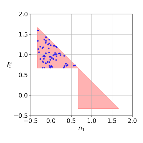
Below, we will study a two-level system weakly coupled to the EM field, i.e. the polarization energy will be several orders less than . For such a case, one must be very careful about binning. Cotton and Miller Cotton and Miller (2016) have suggested that triangular window functions with perform better than square window functions in this regime. Therefore, we have invoked the triangular window function in Eqn. (32) with below.
| (32) |
Here, is Heaviside function. Fig. 1 gives a visual representation of the triangular window function in Eqn. (32). The bottom and upper pink triangles represent areas where and respectively.
To be consistent with the choice of triangular window functions, one must modify the standard protocol in Eqn. (28). Instead of the standard square protocol, assuming we start in excited state , one generates a distribution of initial action variables within the area where (see Eqn. 32) uniformly. Visually, this initialization implies a distribution of inside a triangle centered at in the configuration space, as demonstrated in Fig. 1. The protocol for initializing angle variables is not altered: one sets .
IV.3.3 Advantages and disadvantages of SQC dynamics
Compared with Ehrenfest dynamics, one obvious advantage of SQC dynamics is that the latter can model spontaneous emission when the initial electronic state is . Moreover, the SQC approach must recover detailed balance in the presence of a photonic bath at a given temperatureMiller and Cotton (2015) — provided that the parameter is chosen to be small enough for the binningBellonzi et al. (2016).
At the same time, the disadvantage of the SQC method is that all results are sensitive to the binning width . should be big enough to give enough branching, but also should be small enough to enforce detailed balanceBellonzi et al. (2016). As a result, one must be careful when choosing . Although not relevant here, it is also true that SQC can be unstable for anharmonic potentials.Bellonzi et al. (2016) Lastly, as a practical matter, we have found SQC requires about times more trajectories than Ehrenfest dynamics.
IV.4 Classical Dynamics with Abraham-Lorentz Forces
Although (as shown above) classical electrodynamics with Abraham-Lorentz forces can be useful to model self-interaction, we will not analyze Abraham-Lorentz dynamics further in this paper. Because the correspondence between Ehrenfest dynamics and Abraham-Lorentz dynamics is not unique or generalizable, we feel any further explanation of Abraham-Lorentz equation would be premature. While a Meyer-Miller transformationMeyer and Miller (1979) can reduce a quantum mechanical Hamiltonian into a classical Hamiltonian, the inverse is not possible. Thus, it is not clear how to run classical dynamics with Abraham-Lorentz forces starting from an arbitrary initial superposition state in the basis. For instance, following the approach above in Section II.2, we might set . However, doing so leads to a rate of decay equal to . This result goes to infinity in the limit ; see Fig. 11. Future work may succeed at finding the best correspondence between semiclassical dynamics and the Abraham-Lorentz framework, but such questions will not be the focus of the present paper.
V Simulation Details
V.1 Parameter Regimes
We focus below on Hamiltonians with electronic dipole moment in the range of Cnm/mol ( in Debye) and electronic energy gaps in the range of eV. Other practical parameters are chosen as in Table 1. Two different sets of simulations are run: simulations to capture spontaneous emission (with zero EM field initially) and simulations to capture stimulated emission (with an incoming external finite EM pulse located far away at time zero).
| Quantity | 1D no ABC | 1D with ABC | 3D with ABC |
| 333Eqn. (14) (eV) | 16.46 | 16.46 | 16.46 |
| 444Eqns. (20a, 20b) (Cnm/mol)555As mentioned before, has dimension of C/mol in 1D and Cnm/mol in 3D | 11282 | 11282 | 23917 |
| 666Eqns. (20a, 20b) () | 0.0556 | 0.0556 | 0.0556 |
| 40000 | 200 | 60 | |
| (nm) | 2998 | 89.94 | 89.94 |
| (nm) | -2998 | -89.94 | -89.94 |
| (fs) | |||
| (fs) | 99 | 99 | 500 |
| 777Eqns. (34-35) (nm) | - | 50 | 50 |
| 888Eqns. (34-35) (nm) | - | 84 | 84 |
V.2 Propagation procedure
Equations of motion (Eqns. (21), (22)) are propagated with a Runge-Kutta 4th order solver, and all spatial gradients are evaluated on a real space grid with a two-stencil in 1D and a six-stencil in 3D. Thus, for example, if we consider Eqn. (22) in 1D, in practice we approximate:
| (33) |
etc. Here is a grid index. This numerical method to propagate the EM field (Eqn. (22)) is effectively a finite-difference time-domain (FDTD) methodTaflove (1998); Harris et al. (2011).
V.3 Absorbing boundary condition (ABC)
To run calculations in 3D, absorbing boundary condition (ABC) are required to alleviate the large computational cost. For such a purpose, we invoke a standard, one-dimensional smoothing functionSubotnik and Head-Gordon (2005); Subotnik et al. (2006) :
| (34) |
In 1D, by multiplying the E and B field with after each time step, we force the E and B fields to vanish for .
In 3D, we choose the corresponding smoothing function to be of the form of Eqn. (35),
| (35) |
where , or is exactly the same as Eqn. (34). Note that this smoothing function has cubic (rather than spherical) symmetry.
For the simulations reported below, applying ABC’s allows us to keep only of the grid points in each dimension, so that the computational time is reduced by a factor of in 1D and by a factor of in 3D. Our use of ABC’s is benchmarked in Figs. 2-3, and ABC’s are used implicitly for SQC dynamics in Figs. 6, 10, 11 and 14. ABC’s are also used for the 3D dynamics in Fig. 7.
V.4 Extracting Rates
Our focus below will be on calculating rates of emission; these rates will be subsequently compared with FGR rates. To extract a numerical rate from Ehrenfest or SQC dynamics, we simply calculate the probability to be on the excited state as a function of time () and fit that probability to an exponential decay: . For Ehrenfest dynamics, all results are converged using the default parameters in Table 1. For SQC dynamics, longer simulation times are needed (to ensure ); in practice, we set = 150 fs. Note that, for SQC dynamics, in SQC is calculated by Eqn. (31b) and we sample 2000 trajectories.
VI Results
We now present the results of our simulations and analyze how Ehrenfest and SQC dynamics treat spontaneous emission. The initial state is chosen to be = for Ehrenfest dynamics. We begin in one-dimension.
VI.1 Ehrenfest Dynamics: 1D
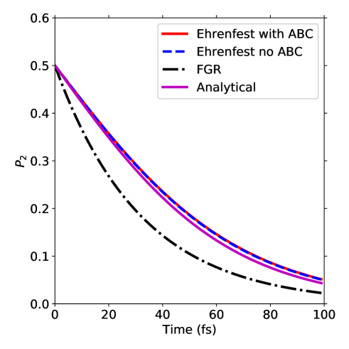
In Fig. 2, we plot for the default parameters in Table 1. Clearly, including ABC’s has no effect on our results. For this set of parameters, Ehrenfest dynamics predicts a decay rate that is slower than Fermi’s Golden Rule (FGR) in Eqn. (3).
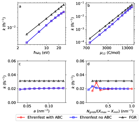
In Fig. 3, we now examine the behavior of Ehrenfest dynamics across a broader parameter regime. In Fig. 3a and 3b, we plot the dependence of the decay rate on the energy difference of electronic states, , and the dipole moment, . Ehrenfest dynamics correctly predicts linear and quadratic dependence, respectively, in agreement with FGR in 1D (see Eqn. (3)). Generally, the fitted decay rate from Ehrenfest dynamics is slower than FGR. As far as the size of the molecule is concerned, in Fig. 3c, we plot the decay rate as a function of the parameter (in Eqn. 20b). Note that our results are independent of molecular size when nm-2. This independence underlies the dipole approximation: when the width of the molecule is much smaller than wavelength of light, , the decay rate should not be dependent on the width of molecule. Note that eV for these simulations, which dictates that results will be dependent on for nm-2. Finally, Fig. 3d should convince the reader that our decay rates are converged with the density of grid points.
VI.1.1 Initial Conditions
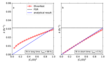
The results above were gathered by setting Let us now address how the initial conditions affect the Ehrenfest rate of spontaneous decay. In Fig. 4 we plot vs. . Here, we differentiate how is extracted, either from a a fit of the long time decay ( fs) or a fit of the short time decay ( fs). Clearly, the decay rates in Fig. 4a and 4b are different, suggesting that the decay of is not purely exponential (see detailed discussion in Appendix); the decay constant is itself a function of time. Moreover, according to Fig. 4, the short time decay rate appears to be linearly dependent on and, in the limit that , both fitted decay rates approach the FGR result. These results suggest that the fitted decay rate satisfies
| (36) |
where is the FGR decay rate. In fact, in the Appendix, we will show that Eqn. (36) can be derived for early time scales ( ) under certain approximations. We also mention that the same failure was observed previously by Tully when investigating the erroneous long time populations predicted by Ehrenfest dynamics.Parandekar and Tully (2005, 2006b); Miller and Cotton (2015)
VI.1.2 Distribution of EM field
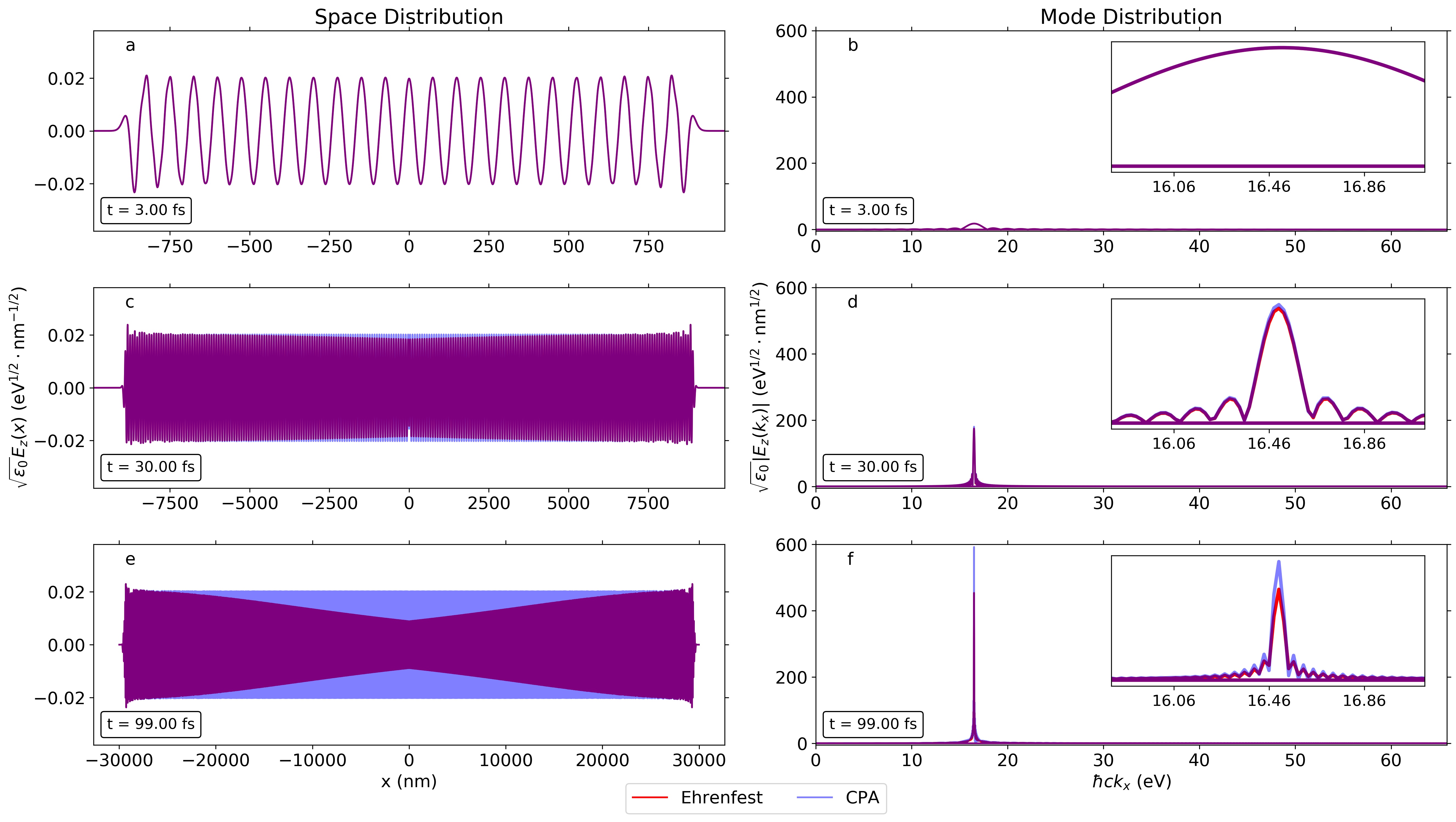
Beyond the electronic subsystem, Ehrenfest dynamics allows us to follow the behavior of the EM field directly. In Fig. 5, we plot the distribution of the EM field at times 3.00 fs (a-b) , 30.00 fs (c-d), and 99.00 fs (e-f) with two methods: Ehrenfest (red lines) and the CPA (light blue lines). On the left hand side, we plot the electric field in real space (); on the right hand side, we plot the EM field in Fourier space (). Here, the Fourier transform is performed over the region , which corresponds to light traveling exclusively to the right. In the insets on the right, we zoom in on the spectra in a small neighborhood of (here, 16.46 eV).
From Fig. 5, we find that Ehrenfest dynamics and the CPA agree for short times. However, for larger times, only Ehrenfest dynamics predicts a decrease in the EM field (corresponding to the spontaneous decay of the signal). This decrease is guaranteed by Ehrenfest dynamics because this method conserves energy. By contrast, because it ignores feedback and violates energy conservation, the CPA does not predict a decrease in the emitted EM field as a function of time (or any spontaneous decay). Thus, overall, as shown in Fig. 5f, the long time EM signal will be a Lorentzian according to Ehrenfest dynamics or a delta-function according to the CPA. These conclusions are unchanged for all values of the initial .
VI.2 SQC: 1D
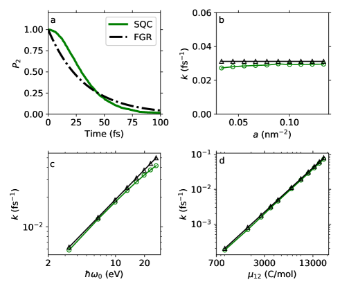
The simulations above have been repeated with SQC dynamics. In Fig. 6a, we plot for a single trajectory that begins on the excited state () for the default parameters (see Table 1). The remaining three sub-figures in Fig. 6 demonstrate the dependence of the fitted decay rate on (b) the molecular width parameter , (c) the electronic excited state energy and (d) the electronic dipole moment . Generally, SQC depends on , and as in a manner similar to Ehrenfest dynamics. However, for the initial condition , the overall SQC decay rate is almost the same as FGR (less than 10 % difference), whereas Ehrenfest dynamics completely fails and predicts . 999For these simulations, we do not consider SQC dynamics as a function of (as in Fig. 4). In practice, for such simulations, we would need to initialize in one representation and measure in another representation, and thus far, we have been unable to recover stable data using the techniques in Ref. Cotton and Miller, 2013b. We believe this failure is likely caused by our own limited experience with SQC.
VI.3 Ehrenfest Dynamics: 3D
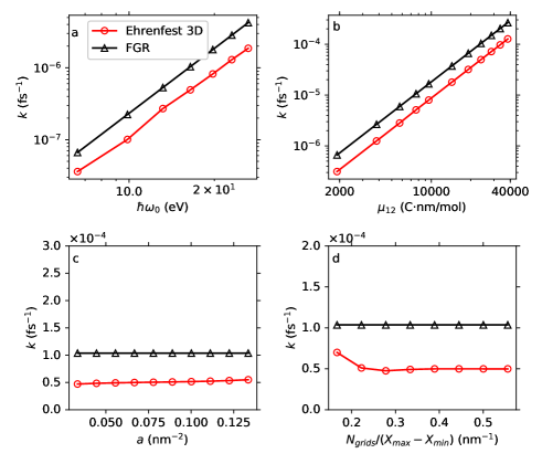
Finally, all of the Ehrenfest simulations above have been repeated in 3D. Overall, as shown in Fig. 7, the results are qualitatively the same as in 1D. However, as was emphasized in Sec. II, the decay rate now depends cubically (and not linearly) on .
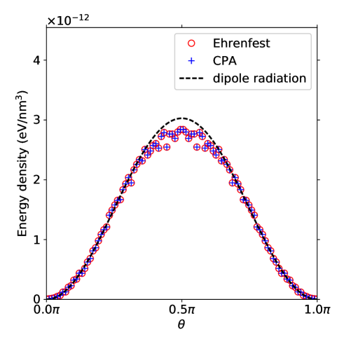
Concerning the radiation of EM field in 3D, in Fig. 8, we plot the energy density versus polar angle at nm when time fs. For such a short time, Ehrenfest dynamics (red ) and CPA (blue ) agree exactly: both results depend on the polar angle through . These results are in very good agreement with theoretical dipole radiation (black line, Eqn. 10). Lastly, in Fig. 9, we plot the energy density as a function of the radial distance from the molecule, while keeping the polar angle fixed at (a) and (b). Again, Ehrenfest dynamics (red ) and the CPA (blue ) agree with each other and give oscillating results that agree with Eqn. (10) for dipole radiation at asymptotically large distances (). Given that the Ehrenfest decay rate does not match spontaneous emission, one might be surprised at the unexpected agreement between Ehrenfest and the CPA dynamics with the classical dipole radiation in Figs. 8-9. In fact, this agreement is somewhat coincidental (depending on initial conditions), as is proved in the Appendix.
VII Discussion
The results above suggest that, for their respective domains of applicability, both Ehrenfest dynamics and SQC can recover spontaneous emission. We will now test this assertion by investigating the response to photo-induced dynamics and dephasing.
VII.1 An incoming pulse in one dimension
To address photo-induced dynamics, we imagine there is an incident pulse at of the form:
| (37) |
Here, is an normalization coefficient with value
The total energy of incident pulse is . The parameter determines the width of the pulse in real space. defines the peak of the pulse in reciprocal space. represents the center of pulse at .
At time zero, the Fourier transform of is:
| (38) |
is the sum of two Gaussians centered at with width . Qualitatively, if , shows two peaks at ; if , resembles a single large packet at . For resonance with the molecule, should be large at (16.46 eV by default).
VII.1.1 Electronic dynamics
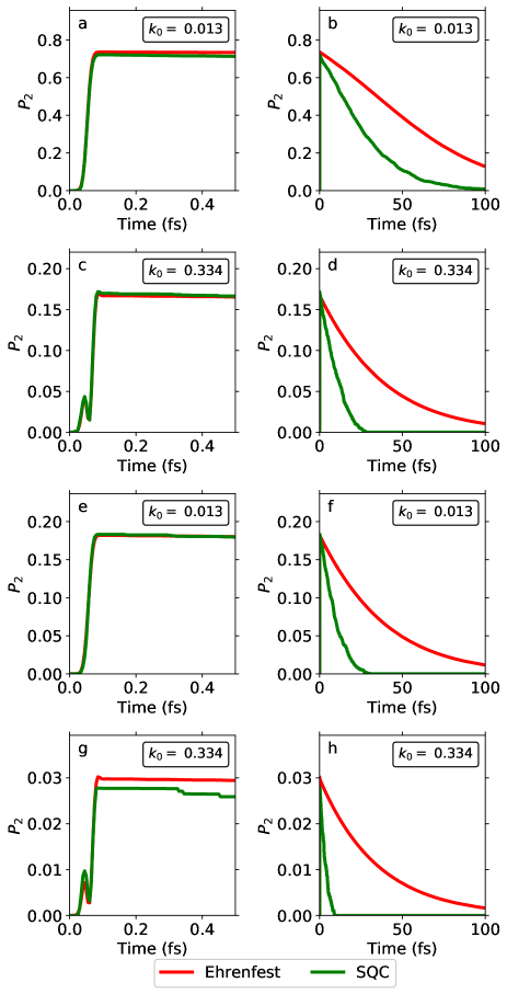
| No. | (keV) | (nm) | ||
|---|---|---|---|---|
| (a-b) | 19.7 | 0.0556 | 0.013 | -15.0 |
| (c-d) | 19.7 | 0.0556 | 0.334 | -15.0 |
| (e-f) | 3.29 | 0.0556 | 0.013 | -15.0 |
| (g-h) | 3.29 | 0.0556 | 0.334 | -15.0 |
In Fig. 10, we plot the electronic population of the excited state as a function of time after exposure to incident pulses of different intensity () and wavevector (); see Eqn. (37). We plot short and long times, on the left and right hand sides, respectively. For strong, resonant pulses, ( keV, ), there is obviously a strong response (see a-b). For strong, off-resonant pulses ( keV, ), obviously the response is weaker. In both situations, SQC (green line) and Ehrenfest dynamics (red line) agree almost exactly for short times. At longer times, however, the SQC value decays times faster than the Ehrenfest dynamics result.
Let us consider now weak pulses. In Fig. 10e-h, we plot the excited state population when the incident pulse is weak ( keV), keeping all other parameters unchanged. Now, there is much less agreement between SQC and Ehrenfest dynamics, especially for long times. Generally, SQC predicts a faster decay rate for than Ehrenfest dynamics for small .
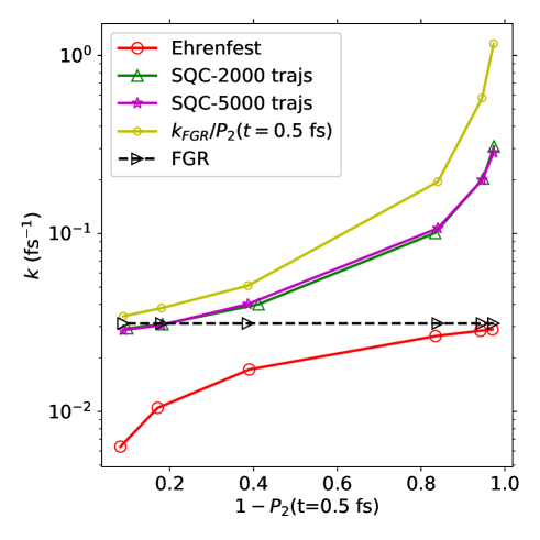
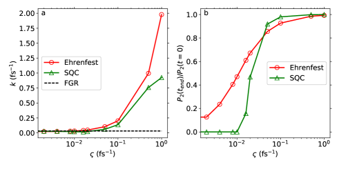
The statement above is quantified in Fig. 11. Here, we vary , which results in a change in the initial absorption (which is quantified by on the -axis). This graph quantifies how the population decay on the excited state depends on the initial condition: the decay of decreases when the initial excited state population decreases. Obviously, this Ehrenfest data is in complete agreement with Fig. 4.
Now, the new piece of data in Fig. 11 is the SQC data. Here, we see that SQC behaves in a manner completely opposite to Ehrenfest: the decay of increases (sometimes dramatically) when the initial excited state population decreases. Thus, for an initial state near , the decay of is unphysically large according to SQC. At the same time, however, the decay of the state is very close to the FGR result (just as noted in Sec. VI). Apparently, by including the zero point energy of the electronic state, SQC is able to include some aspects of true spontaneous decay, but the binning procedure introduces other unnatural consequences. Future work on the proper binning procedure for SQC (triangles, squares, etc. Cotton and Miller (2016)) must address this dilemma.
VII.1.2 Distribution of the EM field
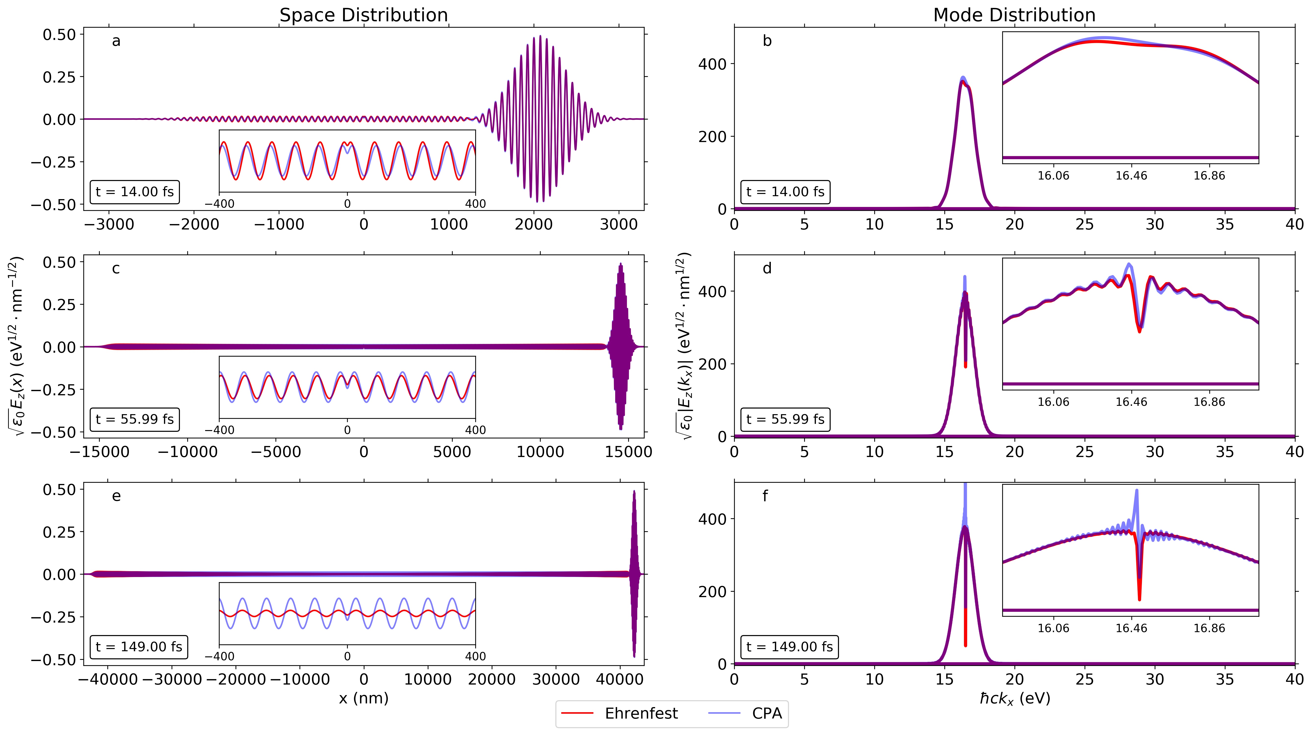
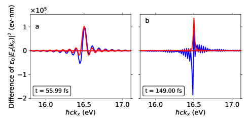
At this point, we should also comment on the EM field that is produced following incident radiation for the two-level system. Effectively, our results are consistent with Fig. 5 above. In Fig. 12, on the left, we plot versus in space at times 14.00 fs (a), 55.99 fs (c) and 149.00 fs (e). On the right hand side, we plot the Fourier transform versus photon energy . As above, we find that, for short times, Ehrenfest dynamics (red lines) and the CPA (light blue lines) are in good agreement. Thereafter, however, the agreement ends because only Ehrenfest dynamics obeys energy conservation. At long times, Ehrenfest dynamics predicts an overall dip (narrow decrease) in the electric field at the frequency of the two-level system (oscillator), while the CPA predicts an overall spike (narrow increase). Thus, if we calculate the absorption spectrum of the molecule by subtracting the total transmitted signal from the freely propagated signal, as in Fig. 13, only the Ehrenfest absorption spectrum is strictly positive; the CPA result makes no sense. This state of affairs reminds us when and how we can use semiclassical theory for understanding light-matter interactions.
Note that, for Fig. 13, we are operating in the linear response regime: the incoming pulse energy is relatively weak. In Appendix C, we plot the absorption spectra for a few different incoming fields and demonstrate that the results are linear with . We also show that standard linear response theory yields a good estimate of the overall lineshape.
VII.2 Dephasing effects
In the present article, we have now shown that semiclassical theories – Ehrenfest and SQC – can both recover some elements of spontaneous emission, which is mostly thought to be a quantum effectMiller (1978); Sukharev and Nitzan (2011). With this claim in mind, however, there is now one final subject that must be addressed, namely the role of dephasing. After all, in a large simulation with an environment, dephasing can and will occur; therefore one must wonder whether or not such dephasing will affect the rate of spontaneous emission.
To answer this question, we have run several simple calculations that replace Eqn. (21) by Eqn. (39),
| (39) |
Thus, we have propagated electron-photon dynamics by altering the electronic equation of motion but keeping the classical EM equations the same. in Eqn. (39) is an empirical dephasing rate: when , there is no dephasing and when there is a finite rate of coherence loss between the two electronic states.
In Fig. 14a, we plot the rate of spontaneous emission as a function of the dephasing rate . When dephasing increases, the coherence between the electronic states is expected to decrease, and so the current should decrease, and thus the rate of spontaneous emission is expected to decrease as well. However, perhaps surprisingly, the fitted rate for establishing equilibrium also increases.
Most importantly, in Fig. 14b, we plot the final population of the excited state . As should be expected, the long term excited state population increases (does not reduce to zero) when dephasing increases with either SQC or Ehrenfest dynamics. This graph highlights the limitations of semiclassical methods: as currently implemented, one cannot include both spontaneous emission and dephasing.
VIII Conclusion
In this article, we have simulated the semiclassical dynamics of light coupled to a two-level electronic system with three different methods: Ehrenfest, the CPA and SQC. Most results have been reported in one dimensional, but we have also considered Ehrenfest dynamics in 3D with absorbing boundary conditions. As far as spontaneous emission is concerned, the CPA cannot consistently recover the effect and violates the energy conservation. That being said, Ehrenfest dynamics do predict spontaneous decay consistently, but only provided that we start in a non-trivial superposition state (with ). Using electronic ZPE, SQC dynamics predicts spontaneous decay even with . Both latter methods yield results fairly close to the correct FGR rate. In all cases, unfortunately, spontaneous emission is destroyed when dephasing is introduced, which represents a fundamental limitation of semiclassical dynamics.
Perhaps most interestingly, we have also studied photo-initiated excited dynamics and, in this case, we find very different dynamics as predicted by the different semiclassical methods. First, as far the EM field is concerned, we have demonstrated that Ehrenfest dynamics can recover the correct absorption spectra, at least qualitatively; at the same time, however, CPA dynamics gives qualitatively incorrect spectra because the method ignores feedback and does not conserve energy. Second, and equally interesting, Ehrenfest dynamics predicts that the overall stimulated decay rate will depend smoothly on initial state but will approach the FGR rate in the weak resonance regime. Vice versa, SQC recovers FGR when but overestimates the stimulated decay rate, sometimes by as much as a factor of 10 in the weak coupling limit. These SQC anomalies should be very important for designing improved binning protocols in the futureCotton and Miller (2016). At present, because the cost of SQC dynamics is roughly times greater than Ehrenfest dynamics and because the method appears to fail for low intensity applied fields, further modification will likely be required before the method can be practical for large-scale simulations.
Looking forward, many questions remain. There are many other semiclassical methods for studying coupled nuclear electronic dynamicsSubotnik et al. (2016); Habershon et al. (2013); Sun and Miller (1997); Cao and Voth (1994); Cotton and Miller (2013b); will these methods give us new insight into electrodynamics? Might we learn more about spontaneous emission by considering ZPE effects through RPMD-like algorithmsPérez De Tudela et al. (2012)? Will different semiclassical methods behave similarly or differently with more than two electronic states? Can we converge multiple-spawningBen-Nun et al. (2000); Martínez (2006); Tao et al. (2009); Levine and Martínez (2009); Kim et al. (2015) and/or MC-TDHBeck et al. (2000); Meyer et al. (2006); Wang and Thoss (2003) calculations and generate exact quantum electrodynamical trajectories so that, in the future, we may benchmark other, less exact, semi-classical approximations? And lastly, , are there other, new and non-intuitive features that will emerge when we study multiple pulses incoming upon a molecule? These questions will be answered in the future.
Acknowledgments
This material is based upon work supported by the (U.S.) Air Force Office of Scientific Research (USAFOSR) PECASE award under AFOSR Grant No. FA9950-13-1-0157 (TL, HTC, JES), AFOSR grant No. FA9550-15-1-0189 (MS), U.S. - Israel Binational Science Foundation Grant No. 2014113 (MS and AN) and the U.S. National Science Foundation Grant No. CHE1665291(AN). This work was also supported by the AMOS program within the Chemical Sciences, Geosciences and Biosciences Division of the Office of Basic Energy Sciences, Office of Science, US Department of Energy (TM). The authors thank Phil Bucksbaum for very stimulating conversations.
Appendix
VIII.1 Connecting Ehrenfest Dynamics with Fermi’s Golden Rule in 1D
We now prove analytically that the spontaneous decay rate of Ehrenfest dynamics in 1D is exactly the FGR result in the limit that the initial excited state population is small ().
For Eqn. (22), we can directly write down an analytic solution for in one dimension using the well known solution for a wave equation with a source:
| (40) |
Here, is the time derivative of . If we average over many different initial electronic populations with different phases, , the average coupling is simpler:
| (41) |
Here, we have denoted Now, for simplicity, suppose the width of the molecule is infinitely small (i.e., a point-dipole approximation), . In such a case, Eqn. (41) can be simplified as:
| (42) |
and therefore, from Eqn. (21),
| (43) |
At this point, we make the weak coupling approximation, and assume that the off-diagonal terms in are infinitely small, so that is a meaningful first order approximation. Eqn. (43) then reads:
| (44) |
where is the FGR spontaneous decay rate in 1D (see Eqn. 3). From Eqn. (44), we can derive the instantaneous transfer rate plus an analytical solution for all times as follows.
First, we consider the instantaneous behavior of Ehrenfest dynamics for within the time scale by integrating Eqn. (44) over the time interval ,
| (45) |
where . The time scale is taken to be much smaller the time scale of spontaneous decay () so that does not change much and . Also, is much larger than the phase oscillating period (), therefore can be viewed as a rapid oscillation and we approximate the integral by
| (46) |
Then we have
| (47) |
As a result, we write Ehrenfest dynamics for in the form of an exponential decay
| (48) |
where the instantaneous decay rate is time-dependent
| (49) |
On the one hand, for short times, the decay rate is proportional to the initial population as shown in Fig. 4b, and we can conclude that Ehrenfest dynamics recovers the FGR rate when .
On the other hand, we may recast Eqn. (44) in terms of the population difference, ,
| (50) |
Just as above, the instantaneous behavior within the time scale can be obtained by
| (51) |
Hence, we find an analytical form for according to Ehrenfest dynamics:
| (52) |
For short times, we take and find that the instantaneous decay rate is also proportional to . For the initial population , as was considered in Fig. 2, the analytical solution becomes . This formula agrees with the numerical result in Fig. 2.
VIII.2 Connecting Ehrenfest Dynamics with classical dipole radiation in 3D
Here, we show that Ehrenfest dynamics agrees with classical dipole radiation at short times assuming that the initial conditions satisfy = . First, consider classical dipole radiation, and let the oscillating dipole (in the -direction) be situated at the origin. The current takes the form and if the dipole width is small enough, the current density is
| (53) |
This is the source that acts as input for Maxwell’s equations and yield classical dipole radiation.
Second, consider Ehrenfest dynamics. Now, takes the form in Eqn. (24). If we take the weak coupling approximation, i.e. we assume that , and we further make the point dipole approximation, , then Eqn. (24) becomes
| (54) |
Lastly, if the initial electronic state satisfies = , then . Thus, this initial electronic state guarantees that Eqns. (53) and (54) will be identical at short times: the EM field from Ehrenfest dynamics will agree with classical dipole radiation exactly. This exact agreement will fail for other initial states or at long times. Even though both methods have the same geometric form, in general, Ehrenfest dynamics would need to be rescaled to match classical dipole radiation in absolute value.
VIII.3 Absorption spectra with different incoming field intensities
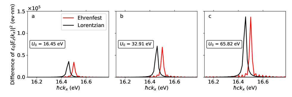
In this subsection, we plot the absorption lineshape for a variety of different incoming fields and prove that the data in Fig. 13 is occurring in the linear regime. Indeed, according to Fig. 15, the overall absorption signal is linearly proportional to the incoming energy . The absorption lineshape can be recovered approximately by simply assuming a Lorentzian signal with width and a uniform fitting for the total norm. Note that there is a small shift in the maximal signal location: according to Ehrenfest dynamics, the peak is centered at (rather than ) where is the time-averaged off-diagonal coupling in the Hamiltonian . See Eqn. (13).
References
- Tokmakoff (2014) A. Tokmakoff, Time-Dependent Quantum Mechanics and Sepctroscopy (2014).
- Törmä and Barnes (2014) P. Törmä and W. L. Barnes, Reports on Progress in Physics 78, 013901 (2014).
- Sukharev and Nitzan (2017) M. Sukharev and A. Nitzan, Journal of Physics: Condensed Matter 29, 443003 (2017).
- Vasa and Lienau (2017) P. Vasa and C. Lienau, ACS Photonics (2017).
- Khitrova et al. (2006) G. Khitrova, H. Gibbs, M. Kira, S. Koch, and A. Scherer, Nature Physics 2, 81 (2006).
- Gibbs et al. (2011) H. Gibbs, G. Khitrova, and S. Koch, Nature Photonics 5, 273 (2011).
- Lodahl et al. (2015) P. Lodahl, S. Mahmoodian, and S. Stobbe, Reviews of Modern Physics 87, 347 (2015).
- Bennett et al. (2017) K. Bennett, M. Kowalewski, and S. Mukamel, Phys. Rev. Lett. 119, 069301 (2017).
- Glownia et al. (2016) J. M. Glownia, A. Natan, J. P. Cryan, R. Hartsock, M. Kozina, M. P. Minitti, S. Nelson, J. Robinson, T. Sato, T. van Driel, G. Welch, C. Weninger, D. Zhu, and P. H. Bucksbaum, Phys. Rev. Lett. 117, 153003 (2016).
- Csesznegi and Grobe (1997) J. R. Csesznegi and R. Grobe, Physical Review Letters 79, 3162 (1997).
- Su et al. (2011) S.-w. Su, Y.-h. Chen, S.-c. Gou, and I. A. Yu, Journal of Physics B: Atomic, Molecular and Optical Physics 44, 165504 (2011), arXiv:1105.6297 .
- Zhang et al. (2012) X. J. Zhang, H. H. Wang, C. Z. Liu, X. W. Han, C. B. Fan, J. H. Wu, and J. Y. Gao, Physical Review A - Atomic, Molecular, and Optical Physics 86, 1 (2012).
- Puthumpally-Joseph et al. (2015) R. Puthumpally-Joseph, O. Atabek, M. Sukharev, and E. Charron, Physical Review A - Atomic, Molecular, and Optical Physics 91, 1 (2015), arXiv:1501.00457 .
- Sukharev and Nitzan (2011) M. Sukharev and A. Nitzan, Physical Review A - Atomic, Molecular, and Optical Physics 84, 1 (2011), arXiv:1104.3325 .
- Smith et al. (2017) H. T. Smith, T. E. Karam, L. H. Haber, and K. Lopata, The Journal of Physical Chemistry C , acs.jpcc.7b03440 (2017).
- Masiello et al. (2005) D. Masiello, E. Deumens, and Y. Öhrn, Physical Review A 71, 032108 (2005).
- Lopata and Neuhauser (2009) K. Lopata and D. Neuhauser, The Journal of chemical physics 131, 014701 (2009).
- Gersten (2005) J. Gersten, “Topics in fluorescence spectroscopy, vol. 8: Radiative decay engineering,” (2005).
- Miller (1978) W. H. Miller, The Journal of Chemical Physics 69, 2188 (1978).
- Cotton and Miller (2013a) S. J. Cotton and W. H. Miller, The Journal of Physical Chemistry A 117, 7190 (2013a).
- Cotton and Miller (2013b) S. J. Cotton and W. H. Miller, The Journal of Chemical Physics 139, 234112 (2013b).
- Schwabl (2007) F. Schwabl, Quantum Mechanics, 4th ed. (Springer-Verlag, Berlin, 2007) p. 306.
- Daboul (1974) J. Daboul, International Journal of Theoretical Physics 11, 145 (1974).
- Griffiths (2012) D. J. Griffiths, Introduction to Electrodynamics, 4th ed. (Pearson, 2012) p. 471.
- Mukamel (1999) S. Mukamel, Principles of Nonlinear Optical Spectroscopy, Oxford series in optical and imaging sciences (Oxford University Press, New York, 1999) pp. 84–92.
- Cohen-Tannoudji et al. (1997) C. Cohen-Tannoudji, J. Dupont-Roc, and G. Grynberg, Photons and Atoms: Introduction to Quantum Electrodynamics (Wiley, 1997) pp. 280–295.
- Lee and Heller (1982) S.-Y. Lee and E. J. Heller, The Journal of Chemical Physics 76, 3035 (1982).
- Cina et al. (2003) J. A. Cina, D. S. Kilin, and T. S. Humble, The Journal of chemical physics 118, 46 (2003).
- Li et al. (2005) X. Li, J. C. Tully, H. B. Schlegel, and M. J. Frisch, Journal of Chemical Physics 123 (2005), 10.1063/1.2008258, arXiv:arXiv:1011.1669v3 .
- Tully (1990) J. C. Tully, The Journal of Chemical Physics 93, 1061 (1990), arXiv:arXiv:1011.1669v3 .
- Nielsen et al. (2000) S. Nielsen, R. Kapral, and G. Ciccotti, Journal of Chemical Physics 112, 6543 (2000).
- Ben-Nun and Martínez (2000) M. Ben-Nun and T. J. Martínez, The Journal of Chemical Physics 112, 6113 (2000).
- Huo and Coker (2012) P. Huo and D. F. Coker, Journal of Chemical Physics 137 (2012), 10.1063/1.4748316.
- Note (1) There is one interesting nuance in this argument. The standard approach for embedding a quantum DOF in a classical environment is the quantum classical Liouville equation(QCLE), which can be approximated by PLDMHuo and Coker (2012) or surface-hopping dynamicsTully (1990). In the present case, for photons interacting with a handful of electronic states, the Hamiltonian is effectively a spin-boson Hamiltonian, which is treated exactly by the QCLE, regardless of the Born-Oppenheimer approximation or any argument about time-scale separation. Nevertheless, in general, we believe that many semi-classical dynamics, especially surface-hopping dynamics, will not be applicable in the present context.
- Note (2) Note that in most applications the Ehrenfest approximation is used to describe coupled electronic and nuclear motions where timescale separation determines the nature of the ensuing dynamics. Here we use this approximation in the spirit of a time dependent Hartree (self consistent field) approximation. Since timescale separation is not invoked, the success of this approach should be scrutinized by its ability to describe physical results, as is done in the present work.
- Parandekar and Tully (2006a) P. V. Parandekar and J. C. Tully, Journal of Chemical Theory and Computation 2, 229 (2006a).
- Smith et al. (1969) E. W. Smith, C. Vidal, and J. Cooper, J. Res. Nat. Bur. Stand. 73 (1969).
- de la Peña and Cetto (2013) L. de la Peña and A. M. Cetto, The Quantum Dice: An Introduction to Stochastic Electrodynamics, Fundamental Theories of Physics (Springer Netherlands, 2013).
- Kim et al. (2008) H. Kim, A. Nassimi, and R. Kapral, J. Comp. Phys. 129, 084102 (2008).
- Meyer and Miller (1979) H. Meyer and W. H. Miller, The Journal of Chemical Physics 70, 3214 (1979).
- Stock and Thoss (1997) G. Stock and M. Thoss, Physical Review Letters 78, 578 (1997), arXiv:z0024 .
- Bellonzi et al. (2016) N. Bellonzi, A. Jain, and J. E. Subotnik, Journal of Chemical Physics 144 (2016), 10.1063/1.4946810.
- Stock (1995) G. Stock, The Journal of Chemical Physics 103, 10015 (1995).
- Miller and Cotton (2016) W. H. Miller and S. J. Cotton, Journal of Chemical Physics 145 (2016), 10.1063/1.4961551.
- Cotton and Miller (2016) S. J. Cotton and W. H. Miller, Journal of Chemical Physics 145 (2016), 10.1063/1.4963914.
- Miller and Cotton (2015) W. H. Miller and S. J. Cotton, “Communication: Note on detailed balance in symmetrical quasi-classical models for electronically non-adiabatic dynamics,” (2015).
- Taflove (1998) A. Taflove, Artec House Inc (1998).
- Harris et al. (2011) N. Harris, L. K. Ausman, J. M. McMahon, D. J. Masiello, and G. C. Schatz, in Computational Nanoscience (Royal Society of Chemistry, 2011) pp. 147–178.
- Subotnik and Head-Gordon (2005) J. E. Subotnik and M. Head-Gordon, Journal of Chemical Physics 123 (2005), 10.1063/1.2000252.
- Subotnik et al. (2006) J. E. Subotnik, A. Sodt, and M. Head-Gordon, Journal of Chemical Physics 125, 1 (2006).
- Parandekar and Tully (2005) P. V. Parandekar and J. C. Tully, The Journal of chemical physics 122, 094102 (2005).
- Parandekar and Tully (2006b) P. V. Parandekar and J. C. Tully, Journal of chemical theory and computation 2, 229 (2006b).
- Note (3) For these simulations, we do not consider SQC dynamics as a function of (as in Fig. 4). In practice, for such simulations, we would need to initialize in one representation and measure in another representation, and thus far, we have been unable to recover stable data using the techniques in Ref. \rev@citealpCotton2013. We believe this failure is likely caused by our own limited experience with SQC.
- Subotnik et al. (2016) J. E. Subotnik, A. Jain, B. Landry, A. Petit, W. Ouyang, and N. Bellonzi, Annual Review of Physical Chemistry 67, 387 (2016).
- Habershon et al. (2013) S. Habershon, D. E. Manolopoulos, T. E. Markland, and T. F. Miller, Annual Review of Physical Chemistry 64, 387 (2013).
- Sun and Miller (1997) X. Sun and W. H. Miller, Journal of Chemical Physics 106, 6346 (1997).
- Cao and Voth (1994) J. Cao and G. A. Voth, The Journal of Chemical Physics 100, 5093 (1994).
- Pérez De Tudela et al. (2012) R. Pérez De Tudela, F. J. Aoiz, Y. V. Suleimanov, and D. E. Manolopoulos, Journal of Physical Chemistry Letters 3, 493 (2012).
- Ben-Nun et al. (2000) M. Ben-Nun, J. Quenneville, and T. J. Martínez, The Journal of Physical Chemistry A 104, 5161 (2000).
- Martínez (2006) T. J. Martínez, Accounts of chemical research 39, 119 (2006).
- Tao et al. (2009) H. Tao, B. G. Levine, and T. J. Martínez, The Journal of Physical Chemistry A 113, 13656 (2009).
- Levine and Martínez (2009) B. G. Levine and T. J. Martínez, The Journal of Physical Chemistry A 113, 12815 (2009).
- Kim et al. (2015) J. Kim, H. Tao, T. J. Martinez, and P. Bucksbaum, Journal of Physics B: Atomic, Molecular and Optical Physics 48, 164003 (2015).
- Beck et al. (2000) M. H. Beck, A. Jäckle, G. Worth, and H.-D. Meyer, Physics reports 324, 1 (2000).
- Meyer et al. (2006) H.-D. Meyer, F. Le Quéré, C. Léonard, and F. Gatti, Chemical physics 329, 179 (2006).
- Wang and Thoss (2003) H. Wang and M. Thoss, The Journal of chemical physics 119, 1289 (2003).