Robust numerical methods for nonlocal (and local) equations of porous medium type.
Part I: Theory

Abstract.

We develop a unified and easy to use framework to study robust fully discrete numerical methods for nonlinear degenerate diffusion equations

$$\partial_{t}u-\mathfrak{L}^{\sigma,\mu}[\varphi(u)]=f\quad\quad\text{in}\quad\quad\mathbb{R}^{N}\times(0,T),$$

where $\mathfrak{L}^{\sigma,\mu}$ is a general symmetric diffusion operator of Lévy type and $\varphi$ is merely continuous and non-decreasing. We then use this theory to prove convergence for many different numerical schemes. In the nonlocal case most of the results are completely new. Our theory covers strongly degenerate Stefan problems, the full range of porous medium equations, and for the first time for nonlocal problems, also fast diffusion equations. Examples of diffusion operators $\mathfrak{L}^{\sigma,\mu}$ are the (fractional) Laplacians $\Delta$ and $-(-\Delta)^{\frac{\alpha}{2}}$ for $\alpha\in(0,2)$, discrete operators, and combinations. The observation that monotone finite difference operators are nonlocal Lévy operators, allows us to give a unified and compact nonlocal theory for both local and nonlocal, linear and nonlinear diffusion equations. The theory includes stability, compactness, and convergence of the methods under minimal assumptions – including assumptions that lead to very irregular solutions. As a byproduct, we prove the new and general existence result announced in [32]. We also present some numerical tests, but extensive testing is deferred to the companion paper [35] along with a more detailed discussion of the numerical methods included in our theory.

1. Introduction

We develop a unified and easy to use framework for monotone schemes of finite difference type for a large class of possibly degenerate, nonlinear, and nonlocal diffusion equations of porous medium type. We then use this theory to prove stability, compactness, and convergence for many different robust schemes. In the nonlocal case most of the results are completely new. The equation we study is

(1.1) $$\begin{cases}\partial_{t}u-\mathfrak{L}^{\sigma,\mu}[\varphi(u)]=f\qquad\qquad&\text{in}\qquad Q_{T}:=\mathbb{R}^{N}\times(0,T),\\ u(x,0)=u_{0}(x)\qquad\qquad&\text{on}\qquad\mathbb{R}^{N},\end{cases}$$

where $u$ is the solution, $\varphi$ is a merely continuous and nondecreasing function, $f=f(x,t)$ some right-hand side, and $T>0$. The diffusion operator $\mathfrak{L}^{\sigma,\mu}$ is given as

(1.2) $$\mathfrak{L}^{\sigma,\mu}:=L^{\sigma}+\mathcal{L}^{\mu}$$

with local and nonlocal (anomalous) parts,

(1.3) $$L^{\sigma}[\psi](x) :=\text{tr}\big{(}\sigma\sigma^{T}D^{2}\psi(x)\big{)},$$

(1.4) $$\mathcal{L}^{\mu}[\psi](x) :=\int_{\mathbb{R}^{N}\setminus\{0\}}\big{(}\psi(x+z)-\psi(x)-z\cdot D\psi(x)\mathbf{1}_{|z|\leq 1}\big{)}\,\mathrm{d}\mu(z),$$

where $\psi\in C_{\textup{c}}^{2}$, $\sigma=(\sigma_{1},....,\sigma_{P})\in\mathbb{R}^{N\times P}$ for $P\in\mathbb{N}$ and $\sigma_{i}\in\mathbb{R}^{N}$, $D$ and $D^{2}$ are the gradient and Hessian, $\mathbf{1}_{|z|\leq 1}$ is a characteristic function, and $\mu$ is a nonnegative symmetric Radon measure.

The assumptions we impose on $\mathfrak{L}^{\sigma,\mu}$ and $\varphi$ are so mild that many different problems can be written in the form (1.1). The assumptions on $\varphi$ allow strongly degenerate Stefan type problems and the full range of porous medium and fast diffusion equations to be covered by (1.1). In the first case e.g. $\varphi(u)=\max(0,au-b)$ for $a\geq 0$ and $b\in\mathbb{R}$ and in the second $\varphi(u)=u|u|^{m-1}$ for any $m\geq 0$. Some physical phenomena that can be modelled by (1.1) are flow in a porous medium (oil, gas, groundwater), nonlinear heat transfer, phase transition in matter, and population dynamics. For more information and examples, we refer to Chapters 2 and 21 in [70] for local problems and to [74, 62, 14, 71] for nonlocal problems.

One important contribution of this paper is that we allow for a very large class of diffusion operators $\mathfrak{L}^{\sigma,\mu}$. This class coincides with the generators of the symmetric Lévy processes. Examples are Brownian motion, $\alpha$-stable, relativistic, CGMY, and compound Poisson processes [9, 69, 7], and the generators include the classical and fractional Laplacians $\Delta$ and $-(-\Delta)^{\frac{\alpha}{2}}$, $\alpha\in(0,2)$ (where $\,\mathrm{d}\mu(z)=c_{N,\alpha}\frac{\,\mathrm{d}z}{|z|^{N+\alpha}}$), relativistic Schrödinger operators $m^{\alpha}I-(m^{2}I-\Delta)^{\frac{\alpha}{2}}$, and surprisingly, also monotone numerical discretizations of $\mathfrak{L}^{\sigma,\mu}$. Since $\sigma$ and $\mu$ may be degenerate or even identically zero, problem (1.1) can be purely local, purely nonlocal, or a combination.

Nonstandard and novel ideas on numerical methods for (1.1) and their analysis are presented in this paper. We will strongly use the fact that our (large) class of diffusion operators contain many of its own monotone approximations. This important observation from [33] is used to interpret discretizations of $\mathfrak{L}^{\sigma,\mu}$ as nonlocal Lévy operators $\mathcal{L}^{\nu}$ which again opens the door for powerful PDE techniques and a unified analysis of our schemes. We consider discretizations of $\mathfrak{L}^{\sigma,\mu}$ of the form

$$\mathcal{L}^{h}[\psi](x)=\sum_{\beta\neq 0}\left(\psi(x+z_{\beta})-\psi(x)\right)\omega_{\beta},$$

or equivalently $\mathcal{L}^{h}=\mathcal{L}^{\nu}$ with $\nu:=\sum_{\beta\not=0}(\delta_{z_{\beta}}+\delta_{z_{-\beta}})\omega_{\beta}$, where $\beta\in\mathbb{Z}^{N}$, the stencil points $z_{\beta}\in\mathbb{R}^{N}\setminus\{0\}$, the weights $\omega_{\beta}\geq 0$, and $z_{-\beta}=-z_{\beta}$ and $\omega_{\beta}=\omega_{-\beta}$. These discretizations are nonpositive in the sense that $\mathcal{L}^{h}[\psi](x_{0})\leq 0$ for any maximum point $x_{0}$ of $\psi\in C_{\textup{c}}^{\infty}(\mathbb{R}^{N})$, and as we will see, they include monotone finite difference quadrature approximations of $\mathfrak{L}^{\sigma,\mu}$. Our numerical approximations of (1.1) will then take the general form

$$\begin{split}U_{\beta}^{j}=U_{\beta}^{j-1}+\Delta t_{j}\big{(}\mathcal{L}_{1}^{h}[\varphi_{1}^{h}(U_{\cdot}^{j})]_{\beta}+\mathcal{L}_{2}^{h}[\varphi_{2}^{h}(U_{\cdot}^{j-1})]_{\beta}+F^{j}_{\beta}\big{)}\end{split}$$

where $U_{\beta}^{j}\approx u(x_{\beta},t_{j})$, $\mathcal{L}^{h}_{i}\approx\mathfrak{L}^{\sigma,\mu}$, $\varphi^{h}_{i}\approx\varphi$, $F_{\beta}^{j}\approx f(x_{\beta},t_{j})$ and $h$ and $\Delta t_{j}$ are the discretization parameters in space and time respectively. By choosing $\varphi^{h}_{1},\varphi^{h}_{2},\mathcal{L}^{h}_{1},\mathcal{L}^{h}_{2}$ in certain ways, we can recover explicit, implicit, $\theta$-methods, and various explicit-implicit methods. In a simple one dimensional case,

$$\partial_{t}u =\varphi(u)_{xx}-(-\partial_{x}^{2})^{\alpha/2}\varphi(u),$$

an example of a discretization in our class is given by

$$U^{j}_{m}=U^{j-1}_{m} +\frac{\Delta t}{h^{2}}\Big{(}\varphi(U^{j}_{m+1})-2\varphi(U^{j}_{m})+\varphi(U^{j}_{m-1})\Big{)}$$

$$+\Delta t\sum_{k\neq 0}\Big{(}\varphi(U^{j-1}_{m+k})-\varphi(U^{j-1}_{m})\Big{)}\int_{(k-\frac{1}{2})h}^{(k+\frac{1}{2})h}\frac{c_{1,\alpha}\,\mathrm{d}z}{|z|^{1+\alpha}}.$$

Our class of schemes include both well-known discretizations and many discretizations that are new in context of (1.1). These new discretizations include higher order discretizations of the nonlocal operators, explicit schemes for fast diffusions, and various explicit-implicit schemes. See the discussion in Sections 2 and 3 and especially the companion paper [35] for more details.

One of the main contributions of this paper is to provide a uniform and rigorous analysis of such numerical schemes in this very general setting, a setting that covers local and nonlocal, linear and nonlinear, non-degenerate and degenerate, and smooth and nonsmooth problems. This novel analysis includes well-posedness, stability, equicontinuity, compactness, and $L^{p}_{\textup{loc}}$-convergence results for the schemes, results which are completely new in some local and most nonlocal cases. Schemes that converge in such general circumstances are often said to be robust. Numerical schemes that are formally consistent are not robust in this generality, i.e. they need not always converge for problems with nonsmooth solutions or can even converge to false solutions. Such issues are seen especially in nonlinear, degenerate and/or low regularity problems. Our general results are therefore only possible because we have (i) identified a class of schemes with good properties (including monotonicity) and (ii) developed the necessary mathematical techniques for this general setting.

A novelty of our analysis is that we are able to present the theory in a uniform, compact, and natural way. By interpreting discrete operators as nonlocal Lévy operators, and the schemes as holding in every point in space, we can use PDE type techniques for the analysis. This is possible because in recent papers [33, 32] we have developed a well-posedness theory for problem (1.1) which in particular allows for the general class of diffusion operators needed here. Moreover, the well-posedness holds for merely bounded distributional or very weak solutions. The fact that we can use such a weak notion of solution will simplify the analysis and make it possible to do a global theory for all the different problems (1.1) and schemes that we consider here. At this point the reader should note that if (1.1) has more regular (bounded) solutions (weak, strong, mild, or classical), then our results still apply because these solutions will coincide with the (unique) distributional solution.

The effect of the Lévy operator interpretation of the discrete operators is that part of our analysis is turned in to a study of semidiscrete in time approximations of (1.1) (cf. (2.5)). A convergence result for these are then obtained from a compactness argument: We prove (i) uniform estimates in $L^{1}$ and $L^{\infty}$ and space/time translation estimates in $L^{1}$/$L^{1}_{\textup{loc}}$, (ii) compactness in $C([0,T];L^{1}_{\textup{loc}}(\mathbb{R}^{N}))$ via the Arzelà-Ascoli and Kolmogorov-Riesz theorems, (iii) limits of convergent subsequences are distributional solutions via stability results for (1.1), and finally (iv) full convergence of the numerical solutions by (ii), (iii), and uniqueness for (1.1). The proofs of the various a priori estimates are done from scratch using new, efficient, and nontrivial approximation arguments for nonlinear nonlocal problems.

To complete our proofs, we also need to connect the results for the semi-discrete scheme defined on the whole space with the fully discrete scheme defined on a spatial grid. We observe here that this part is easy for uniform grids where we prove an equivalence theorem under natural assumptions on discrete operators: Piecewise constant interpolants of solutions of the fully discrete scheme coincides with solutions of the corresponding semi-discrete scheme with piecewise constant initial data (see Proposition 2.13). Nonuniform grids is a very interesting case that we leave for future work.

The nonlocal approach presented in this paper gives a uniform way of representing local, nonlocal and discrete problems, different schemes and equations; compact, efficient, and easy to understand PDE type arguments that work for very different problems and schemes; new convergence results for local and nonlocal problems; and it is very natural since the difference quadrature approximations $\mathcal{L}^{h}$ are nonlocal operators of the form (1.4), even when equation (1.1) is local.

We also mention that a consequence of our convergence and compactness theory is the existence of distributional solutions of the Cauchy problem (1.1).

Related work. In the local linear case, when $\varphi(u)=u$ and $\mu\equiv 0$ in (1.1), numerical methods and analysis can be found in undergraduate text books. In the nonlinear case there is a very large literature so we will focus only on some developments that are more relevant to this paper. For porous medium nonlinearities ($\varphi(u)=u|u|^{m-1}$ with $m>1$), there are early results on finite element and finite-difference interface tracking methods in [67] and [39] (see also [64]). There is extensive theory for finite volume schemes, see [51, Section 4] and references therein for equations with locally Lipschitz $\varphi$. For finite element methods there is a number of results, including results for fast diffusions ($m\in(0,1)$), Stefan problems, convergence for strong and weak solutions, discontinuous Galerkin methods, see e.g. [68, 48, 49, 47, 76, 66, 63]. Note that the latter paper considers the general form of (1.1) with $\mathfrak{L}^{\sigma,\mu}=\Delta$ and provides a convergence analysis in $L^{1}$ using nonlinear semi-group theory. A number of results on finite difference methods for degenerate convection-diffusion equations also yield results for (1.1) in special cases, see e.g. [50, 13, 59, 57]. In particular the results of [50, 59] imply our convergence results for a particular scheme when $\varphi$ is locally Lipschitz, $\mathfrak{L}^{\sigma,\mu}=\Delta$, and solutions have a certain additional BV regularity. Finally, we mention very general results on so-called gradient schemes [42, 43, 46] for porous medium equations or more general doubly or triply degenerate parabolic equations.

In the nonlocal case, the literature is more recent and not so extensive. For linear equations in the whole space, finite difference methods have been studied in e.g. [24, 53, 54, 19]. An important but different line of research concerns problems on bounded domains, see e.g. [38, 11, 65, 1, 25]. This direction will not be discussed further in this paper. Some early numerical results for nonlocal problems came for finite difference quadrature schemes for Bellman equations and fractional conservation laws, see [56, 17, 10] and [40]. For the latter case discontinuous Galerkin and spectral methods were later studied in [23, 21, 75]. The first results that include nonlinear nonlocal versions of (1.1) was probably given in [20]. Here convergence of finite difference quadrature schemes was proven for a convection-diffusion equation. This result is extended to more general equations and error estimates in [22] and a higher order discretization in [45]. In some cases our convergence results follow from these results (for two particular schemes, $\sigma=0$, and $\varphi$ locally Lipschitz). However, the analysis there is different and more complicated since it involves entropy solutions and Kružkov doubling of variables arguments.

In the purely parabolic case (1.1), the behaviour of the solutions and the underlying theory is different from the convection-diffusion case (especially so in the nonlocal case, see e.g. [27, 28, 72, 26, 73] and [44, 18, 3, 20, 5, 55]). It is therefore important to develop numerical methods and analysis that are specific for this setting. The first numerical results for Fractional Porous Medium Equations seem to be [31, 37] which are based on the extension method [15]. The present paper is another step in this direction, possibly the first not to use the extension method in this setting.

Outline. The assumptions, numerical schemes, and main results are given in Section 2. In Section 3 we provide many concrete examples of schemes that satisfy the assumptions of Section 2. We also show some numerical results for a nonlocal Stefan problem with non-smooth solutions. The proofs of the main results are given in Section 4, while some auxiliary results are proven in our final section, Section 5.

In the companion paper [35] there is a more complete discussion of the family of numerical methods. It includes more discretizations of the operator $\mathfrak{L}^{\sigma,\mu}$, more schemes, and many numerical examples. There we also provide proofs and explanations for why the different schemes satisfy the (technical) assumptions of this paper.

2. Main results

The main results of this paper are presented in this section. They include the definition of the numerical schemes, their consistency, monotonicity, stability, and convergence of numerical solutions towards distributional solutions of the porous medium type equation (1.1).

2.1. Assumptions and preliminaries

The assumptions on (1.1) are

($$\textup{A}_{\varphi} \varphi:\mathbb{R}\to\mathbb{R}\text{ is nondecreasing and continuous};$$)

($$\textup{A}_{f} f\text{ is measurable and }\int_{0}^{T}\big{(}\|f(\cdot,t)\|_{L^{1}(\mathbb{R}^{N})}+\|f(\cdot,t)\|_{L^{\infty}(\mathbb{R}^{N})}\big{)}\,\mathrm{d}t<\infty;$$)

($$\textup{A}_{u_{0}} u_{0}\in L^{1}(\mathbb{R}^{N})\cap L^{\infty}(\mathbb{R}^{N});\text{ and}$$)

$$\mu\text{ is a nonnegative symmetric Radon measure on }\mathbb{R}^{N}\setminus\{0\}\text{ satisfying}$$

$$\quad\int_{|z|\leq 1}|z|^{2}\,\mathrm{d}\mu(z)+\int_{|z|>1}1\,\mathrm{d}\mu(z)<\infty.$$

Sometimes we will need stronger assumptions than ($\textup{A}_{\varphi}$) and (2.1):

($$\textup{Lip}_{\varphi} \varphi:\mathbb{R}\to\mathbb{R}\text{ is nondecreasing and locally Lipschitz; and}$$)

$$\nu\text{ is a nonnegative symmetric Radon measure satisfying }\nu(\mathbb{R}^{N})<\infty.$$

Remark 2.1.

1. Without loss of generality, we can assume $\varphi(0)=0$ (replace $\varphi(u)$ by $\varphi(u)-\varphi(0)$), and when ($\textup{Lip}_{\varphi}$) holds, that $\varphi$ is globally Lipschitz (since $u$ is bounded). In the latter case we let $L_{\varphi}$ denote the Lipschitz constant.

2. Under assumption (2.1), for any $p\in[1,\infty]$ and any $\psi\in C_{\textup{c}}^{\infty}(\mathbb{R}^{N})$,

   (2.1) $$\|\mathfrak{L}^{\sigma,\mu}[\psi]\|_{L^{p}}\leq c\|D^{2}\psi\|_{L^{p}}\Big{(}|\sigma|^{2}+\int_{|z|\leq 1}|z|^{2}\,\mathrm{d}\mu(z)\Big{)}+2\|\psi\|_{L^{p}}\int_{|z|>1}\,\mathrm{d}\mu(z).$$

3. Assumption ($\textup{A}_{f}$) is equivalent to requiring $f\in L^{1}(0,T;L^{1}(\mathbb{R}^{N})\cap L^{\infty}(\mathbb{R}^{N}))$, an iterated $L^{P}$-space as in e.g. [8]. Note that $L^{1}(0,T;L^{1}(\mathbb{R}^{N}))=L^{1}(Q_{T})$.

Definition 2.1 (Distributional solution).

Let $u_{0}\in L_{\textup{loc}}^{1}(\mathbb{R}^{N})$ and $f\in L_{\textup{loc}}^{1}(Q_{T})$. Then $u\in L_{\textup{loc}}^{1}(Q_{T})$ is a distributional (or very weak) solution of (1.1) if for all $\psi\in C_{\textup{c}}^{\infty}(\mathbb{R}^{N}\times[0,T))$, $\varphi(u)\mathfrak{L}^{\sigma,\mu}[\psi]\in L^{1}(Q_{T})$ and

(2.2) $$\int_{0}^{T}\int_{\mathbb{R}^{N}}\big{(}u\partial_{t}\psi+\varphi(u)\mathfrak{L}^{\sigma,\mu}[\psi]+f\psi\big{)}\,\mathrm{d}x\,\mathrm{d}t+\int_{\mathbb{R}^{N}}u_{0}(x)\psi(x,0)\,\mathrm{d}x=0$$

Note that $\varphi(u)\mathfrak{L}^{\sigma,\mu}[\psi]\in L^{1}$ if e.g. $u\in L^{\infty}$ and $\varphi$ continuous. Distributional solutions are unique in $L^{1}\cap L^{\infty}$.

Theorem 2.2 (Theorem 3.1 [32]).

Assume ($\textup{A}_{\varphi}$), ($\textup{A}_{f}$), ($\textup{A}_{u_{0}}$), and (2.1). Then there is at most one distributional solution $u$ of (1.1) such that $u\in L^{1}(Q_{T})\cap L^{\infty}(Q_{T})$.

2.2. Numerical schemes without spatial grids

Let $\mathcal{T}_{\Delta t}^{T}=\{t_{j}\}_{j=0}^{J}$ be a nonuniform grid in time such that $0=t_{0}<t_{1}<\ldots<t_{J}=T$. Let $\mathbb{J}:=\{1,\ldots,J\}$, and denote time steps by

(2.3) $$\Delta t_{j}=t_{j}-t_{j-1}\quad\textup{for every}\quad j\in\mathbb{J},\quad\textup{and}\quad\Delta t=\max_{j\in\mathbb{J}}\{\Delta t_{j}\}.$$

For $j\in\mathbb{J}$ and $x\in\mathbb{R}^{N}$, we define

(2.4) $$F(x,t_{j}):=F^{j}(x)=\frac{1}{\Delta t_{j}}\int_{t_{j}-\Delta t_{j}}^{t_{j}}f(x,t)\,\mathrm{d}t,$$

and we define our time discretized scheme, for $h>0$, as

(2.5) $$\begin{cases}U_{h}^{j}(x)=U_{h}^{j-1}(x)+\Delta t_{j}\Big{(}\mathcal{L}_{1}^{h}[\varphi_{1}^{h}(U_{h}^{j})](x)+\mathcal{L}_{2}^{h}[\varphi_{2}^{h}(U_{h}^{j-1})](x)+F^{j}(x)\Big{)}\\[5.69046pt] U_{h}^{0}(x)=u_{0}(x)\end{cases}$$

where, formally, $U_{h}^{j}(x)\approx u(x,t_{j})$, $\frac{U_{h}^{j}(x)-U_{h}^{j-1}(x)}{\Delta t_{j}}\approx\partial_{t}u(x,t_{j})$, and

$$\mathcal{L}_{1}^{h}[\varphi_{1}^{h}(U_{h}^{j})](x)+\mathcal{L}_{2}^{h}[\varphi_{2}^{h}(U_{h}^{j-1})](x)\approx\mathfrak{L}^{\sigma,\mu}[\varphi(u)](x,t_{j}).$$

Typically $\varphi_{1}^{h}=\varphi=\varphi_{2}^{h}$, but when $\varphi$ is not Lipschitz, we have to approximate it by a Lipschitz $\varphi_{2}^{h}$ to get a monotone explicit method [35]. Let $\varphi_{1}^{h}=\varphi=\varphi_{2}^{h}$. Depending on the choice of $\mathcal{L}_{1}^{h}$ and $\mathcal{L}_{2}^{h}$, we can then get many different schemes:

1. Discretizing separately the different parts of the operator

   $$\mathfrak{L}^{\sigma,\mu}=L^{\sigma}+\mathcal{L}^{\mu}_{\text{sing}}+\mathcal{L}^{\mu}_{\text{bnd}},$$

   e.g. the local, singular nonlocal, and bounded nonlocal parts, corresponds to different choices for $\mathcal{L}_{1}^{h}$ and $\mathcal{L}_{2}^{h}$. Typical choices here are finite difference and numerical quadrature methods, see Section 3 for several examples.

2. Explicit schemes ($\theta=0$), implicit schemes ($\theta=1$), or combinations like Crank-Nicholson ($\theta=\frac{1}{2}$), follow by the choices

   $$\mathcal{L}_{1}^{h}=\theta\mathcal{L}^{h}\qquad\text{and}\qquad\mathcal{L}_{2}^{h}=(1-\theta)\mathcal{L}^{h}.$$

3. Combinations of type (1) and (2) schemes, e.g. implicit discretization of the unbounded part of $\mathfrak{L}^{\sigma,\mu}$ and explicit discretization of the bounded part.

Finally, we mention that our schemes and results may easily be extended to handle any finite number of $\varphi_{1}^{h},\dots,\varphi_{m}^{h}$ and $\mathcal{L}_{1}^{h},\dots,\mathcal{L}_{m}^{h}$.

Definition 2.2 (Consistency).

We say that the scheme (2.5) is consistent if, for $\varphi_{1},\varphi_{2},\varphi$ satisfying ($\textup{A}_{\varphi}$), $\mu$ (2.1), and $\mathfrak{L}^{\sigma,\mu}_{1}$, $\mathfrak{L}^{\sigma,\mu}_{2}$, $\mathfrak{L}^{\sigma,\mu}$ of the form (1.2)–(1.4),

1. $\mathfrak{L}^{\sigma,\mu}_{1}[\varphi_{1}(\phi)]+\mathfrak{L}^{\sigma,\mu}_{2}[\varphi_{2}(\phi)]=\mathfrak{L}^{\sigma,\mu}[\varphi(\phi)]$ in $\mathcal{D}^{\prime}(Q_{T})$ for $\phi\in L^{1}(\mathbb{R}^{N})\cap L^{\infty}(\mathbb{R}^{N})$,

2. for all $\psi\in C_{\textup{c}}^{\infty}(\mathbb{R}^{N})$ and some $k_{1},k_{2}\geq 0$,

   $$\|\mathcal{L}_{i}^{h}[\psi]-\mathfrak{L}^{\sigma,\mu}_{i}[\psi]\|_{L^{1}(\mathbb{R}^{N})}\leq\|\psi\|_{W^{k_{i},1}(\mathbb{R}^{N})}o_{h}(1)\stackrel{{\scriptstyle h\to 0^{+}}}{{\longrightarrow}}0\qquad\textup{for}\qquad i=1,2,$$

3. $\varphi_{1}^{h},\varphi_{2}^{h}\to\varphi_{1},\varphi_{2}$ locally uniformly as $h\to 0^{+}$.

Remark 2.3.

In view of step 4) in the proof of Lemma 4.8, condition (ii) can be replaced by the following more general consistency condition

$$\|\mathcal{L}_{i}^{h}[\psi(\cdot,t)]-\mathfrak{L}^{\sigma,\mu}_{i}[\psi(\cdot,t)]\|_{C([0,T];L^{1}(\mathbb{R}^{N}))}\stackrel{{\scriptstyle h\to 0^{+}}}{{\longrightarrow}}0\qquad\textup{for all}\qquad\psi\in C_{\textup{c}}^{\infty}(Q_{T})$$

and for $i=1,2$. This concept of consistency holds for all the discretizations we are considering; see also the companion paper [35].

We will focus on discrete operators $\mathcal{L}_{i}^{h}$, $i=1,2$ in the following class:

Definition 2.3.

An operator $\mathcal{L}$ is said to be

1. in the class (2.1) if $\mathcal{L}=\mathcal{L}^{\nu}$ for a measure $\nu$ satisfying (2.1); and

2. discrete if

   $$\nu=\sum_{\beta\not=0}(\delta_{z_{\beta}}+\delta_{z_{-\beta}})\omega_{\beta}$$

   for $z_{\beta}=-z_{-\beta}\in\mathbb{R}^{N}$ and $\omega_{\beta}=\omega_{-\beta}\in\mathbb{R}_{+}$ such that $\sum_{\beta\not=0}\omega_{\beta}<\infty$.

3. $\mathcal{S}=\{z_{\beta}\}_{\beta}$ is called the stencil and $\{\omega_{\beta}\}_{\beta}$ the weights of the discretization.

All operators in the class (2.1) are nonpositive operators, in particular they are integral or quadrature operators with positive weights. The results presented in this section hold for any operator in the class (2.1). However, in practice, when dealing with numerical schemes, the operators will additionally be discrete. Moreover, when the scheme (2.5) has an explicit part, that is $\nu_{2}^{h}$ and $\varphi_{2}^{h}$ are not simultaneously zero, we need to assume that $\varphi_{2}^{h}$ satisfies ($\textup{Lip}_{\varphi}$) and impose the following CFL-type condition to have a monotone scheme:

(CFL) $$\Delta tL_{\varphi_{2}^{h}}\nu_{2}^{h}(\mathbb{R}^{N})\leq 1,$$

where we recall that $L_{\varphi_{2}^{h}}$ is the Lipschitz constant of $\varphi_{2}^{h}$ (see Remark 2.1). Note that this condition is always satisfied for an implicit method where $\nu_{2}^{h}\equiv 0$. The typical assumptions on the scheme (2.5) are then:

($$\textup{A}_{\textup{NS}} \begin{cases}\text{ $\mathcal{L}_{1}^{h},\mathcal{L}_{2}^{h}$ are in the class \eqref{nuas} with respective measures $\nu_{1}^{h},\nu_{2}^{h}$,}\\[5.69046pt] \text{$\varphi_{1}^{h},\varphi_{2}^{h}$ satisfy \eqref{phias}, \eqref{philipas} respectively, and}\\[5.69046pt] \text{$\Delta t>0$ is such that \eqref{CFL} holds.}\end{cases}$$)

Theorem 2.4 (Existence and uniqueness).

Assume ($\textup{A}_{\textup{NS}}$), ($\textup{A}_{f}$), and ($\textup{A}_{u_{0}}$). Then there exists a unique a.e.-solution $U_{h}^{j}\in L^{1}(\mathbb{R}^{N})\cap L^{\infty}(\mathbb{R}^{N})$ of the scheme (2.5).

Remark 2.5.

Since $U_{h}^{j}$ is a Lebesgue measurable function, it is not immediately clear that $\varphi_{1}^{h}(U_{h}^{j}),\varphi_{2}^{h}(U_{h}^{j-1})$ are $\nu_{1}^{h},\nu_{2}^{h}$-measurable and $\mathcal{L}_{1}^{h}[\varphi_{1}^{h}(U_{h}^{j})],\mathcal{L}_{2}^{h}[\varphi_{2}^{h}(U_{h}^{j-1})]$ are pointwisely well-defined. However, we could simply consider a Borel measurable a.e. representative of $U_{h}^{j}$; see also Remark 2.1 (1) and (2) in [4] for a discussion.

Theorem 2.6 (A priori estimates).

Assume ($\textup{A}_{\textup{NS}}$), ($\textup{A}_{f}$), and ($\textup{A}_{u_{0}}$). Let $U^{j}_{h},V^{j}_{h}$ be solutions of the scheme (2.5) with data $u_{0},v_{0}$ and $f,g$. Then:

1. (Monotonicity) If $u_{0}(x)\leq v_{0}(x)$ and $f(x,t)\leq g(x,t)$, then $U_{h}^{j}(x)\leq V_{h}^{j}(x)$.

2. ($L^{1}$-stability) $\|U_{h}^{j}\|_{L^{1}(\mathbb{R}^{N})}\leq\|u_{0}\|_{L^{1}(\mathbb{R}^{N})}+\int_{0}^{t_{j}}\|f(\cdot,\tau)\|_{L^{1}(\mathbb{R}^{N})}\,\mathrm{d}\tau$.

3. ($L^{\infty}$-stability) $\|U_{h}^{j}\|_{L^{\infty}(\mathbb{R}^{N})}\leq\|u_{0}\|_{L^{\infty}(\mathbb{R}^{N})}+\int_{0}^{t_{j}}\|f(\cdot,\tau)\|_{L^{\infty}(\mathbb{R}^{N})}\,\mathrm{d}\tau$.

4. (Conservativity) If $\varphi_{1}^{h}$ additionally satisfies ($\textup{Lip}_{\varphi}$),

   $$\int_{\mathbb{R}^{N}}U_{h}^{j}(x)\,\mathrm{d}x=\int_{\mathbb{R}^{N}}u_{0}(x)\,\mathrm{d}x+\int_{0}^{t_{j}}\int_{\mathbb{R}^{N}}f(x,\tau)\,\mathrm{d}x\,\mathrm{d}\tau.$$

Remark 2.7.

By (b), (c), and interpolation, the scheme is $L^{p}$-stable for $p\in[1,\infty]$.

The scheme is also $L^{1}$-contractive and equicontinuous in time. Combined, these two results imply time-space equicontinuity and compactness of the scheme, a key step in our proof of convergence.

Theorem 2.8 ($L^{1}$-contraction).

Under the assumptions of Theorem 2.6,

$$\int_{\mathbb{R}^{N}}(U_{h}^{j}-V_{h}^{j})^{+}(x)\,\mathrm{d}x\leq\int_{\mathbb{R}^{N}}(u_{0}-v_{0})^{+}(x)\,\mathrm{d}x+\int_{0}^{t_{j}}\int_{\mathbb{R}^{N}}(f-g)^{+}(x,\tau)\,\mathrm{d}x\,\mathrm{d}\tau.$$

For the equicontinuity in space and time we need a modulus of continuity:

(2.6) $$\Lambda_{K}(\zeta) :=2\,\lambda_{u_{0},f}(\zeta^{\frac{1}{3}})+C_{K}(\zeta^{\frac{1}{3}}+\zeta),$$

where

(2.7) $$\lambda_{u_{0},f}(\zeta):=\sup_{|\xi|\leq\zeta}\Big{(}\|u_{0}-u_{0}(\cdot+\xi)\|_{L^{1}(\mathbb{R}^{N})}+\|f-f(\cdot+\xi,\cdot)\|_{L^{1}(Q_{T})}\Big{)},$$

(2.10) $$C_{K}:=c|K|\sup_{\scriptsize\begin{array}[]{c}h<1,\\ i=1,2\end{array}}\!\!\Big{(}1+\sup_{|\zeta|\leq M_{u_{0},f}}\!\!\!|\varphi_{i}^{h}(\zeta)|\Big{)}\Big{(}1+\int_{|z|>0}|z|^{2}\wedge 1\ \,\mathrm{d}\nu_{i}^{h}(z)\Big{)}$$

for some constant $c\geq 1$, $a\wedge b:=\min\{a,b\}$, $K\subset\mathbb{R}^{N}$ compact with Lebesgue measure $|K|$, and $M_{u_{0},f}:=\|u_{0}\|_{L^{\infty}(\mathbb{R}^{N})}+\int_{0}^{T}\|f(\cdot,\tau)\|_{L^{\infty}(\mathbb{R}^{N})}\,\mathrm{d}\tau$. In view of (2.10), we also need to assume a uniform Lévy condition on the approximations,

($$\textup{A}_{\nu^{h}} \sup_{\scriptsize\begin{array}[]{c}h<1,\\ i=1,2\end{array}}\int_{|z|>0}|z|^{2}\wedge 1\ \,\mathrm{d}\nu_{i}^{h}(z)<+\infty.$$)

Remark 2.9.

Condition ($\textup{A}_{\nu^{h}}$) is in general very easy to check. For example it follows from pointwise consistency of $\mathcal{L}_{i}^{h}$ as we will see in [35].

Theorem 2.10 (Equicontinuity in time).

Assume ($\textup{A}_{f}$) and ($\textup{A}_{u_{0}}$), and let (2.5) be a consistent scheme satisfying ($\textup{A}_{\textup{NS}}$) and ($\textup{A}_{\nu^{h}}$). Then, for all $j,k\in\mathbb{J}$ such that $j-k\geq 0$ and all compact sets $K\subset\mathbb{R}^{N}$,

$$\begin{split}&\|U_{h}^{j}-U_{h}^{j-k}\|_{L^{1}(K)}\leq\Lambda_{K}(t_{j}-t_{j-k})+|K|\int_{t_{j-k}}^{t_{j}}\|f(\cdot,\tau)\|_{L^{\infty}(\mathbb{R}^{N})}\,\mathrm{d}\tau,\end{split}$$

where $\Lambda_{K}$ is defined in (2.6).

The main result regarding convergence of numerical schemes without spatial grids will be presented in a continuous in time and space framework. For that reason, let us define the piecewise linear time interpolant $\widetilde{U}_{h}$, for $(x,t)\in Q_{T}$, as

(2.11) $$\begin{split}\widetilde{U}_{h}(x,t)&:=U_{h}^{0}(x)\mathbf{1}_{\{t_{0}\}}(t)\\ &\quad+\sum_{j=1}^{J}\mathbf{1}_{(t_{j-1},t_{j}]}(t)\Big{(}U_{h}^{j-1}(x)+\frac{t-t_{j-1}}{t_{j}-t_{j-1}}\big{(}U_{h}^{j}(x)-U_{h}^{j-1}(x)\big{)}\Big{)}.\end{split}$$

Theorem 2.11 (Convergence).

Assume ($\textup{A}_{f}$), ($\textup{A}_{u_{0}}$), $\Delta t=o_{h}(1)$, and for all $h>0$, let $U^{j}_{h}$ be the solution of a consistent scheme (2.5) satisfying ($\textup{A}_{\textup{NS}}$) and ($\textup{A}_{\nu^{h}}$). Then there exists a unique distributional solution $u\in L^{1}(Q_{T})\cap L^{\infty}(Q_{T})\cap C([0,T];L_{\textup{loc}}^{1}(\mathbb{R}^{N}))$ of (1.1) and

$$\widetilde{U}_{h}\to u\quad\text{in}\quad C([0,T];L_{\textup{loc}}^{1}(\mathbb{R}^{N}))\quad\text{as}\quad h\to 0^{+}.$$

Convergence of subsequences follows from compactness and full convergence follows from stability and uniqueness of the limit problem (1.1). The detailed proofs of Theorems 2.4, 2.6, and 2.8–2.11 can be found in Sections 4.1–4.3.

Remark 2.12.

In this paper, we use piecewise linear interpolation to ensure that $\widetilde{U}_{h}$ belongs to $C([0,T];L_{\textup{loc}}^{1}(\mathbb{R}^{N}))$. Moreover, we obtain an equicontinuity result in time uniformly in $\Delta t=o_{h}(1)$. Compactness and convergence then follows from Arzelà-Ascoli and Kolmogorov-Riesz type compactness results (see e.g. [36]).

In most of the related literature piecewise constant interpolation is used. In this case there is no convergence in $C([0,T];L_{\textup{loc}}^{1}(\mathbb{R}^{N}))$, but one can use Kružkov type interpolation lemmas along with the Kolmogorov-Riesz compactness theorem to get convergence in $L_{\textup{loc}}^{1}(Q_{T})$. Consult e.g. [60] for the vanishing viscosity limit of scalar conservation laws; [58] for finite-difference approximations of convection-diffusion equations; [6] for finite volume approximations of nonlinear elliptic-parabolic problems; and [22] for finite volume approximations of nonlocal convection-diffusion equations. Yet another approach is discontinuous versions of the Arzelà-Ascoli compactness theorem (combined with Kolmogorov-Riesz) to get convergence in $L^{\infty}((0,T);L_{\textup{loc}}^{1}(\mathbb{R}^{N}))$; see the appendix of [41].

2.3. Numerical schemes on uniform spatial grids

To get computable schemes, we need to introduce spatial grids. For simplicity we restrict to uniform grids. Since our discrete operators have weights and stencils not depending on the position $x$, all results then become direct consequences of the results in Section 2.2.

Let $h>0$, $R_{h}=h(-\frac{1}{2},\frac{1}{2}]^{N}$, and $\mathcal{G}_{h}$ be the uniform spatial grid

$$\mathcal{G}_{h}:=h\mathbb{Z}^{N}=\{x_{\beta}:=h\beta:\beta\in\mathbb{Z}^{N}\}.$$

Note that any discrete (2.1)-class operator $\mathcal{L}^{h}$ with stencil $\mathcal{S}\subset\mathcal{G}_{h}$ is defined by

$$\mathcal{L}^{h}[\psi](x_{\beta})=\mathcal{L}^{h}[\psi]_{\beta}=\sum_{\gamma\not=0}(\psi(x_{\beta}+z_{\gamma})-\psi(x_{\beta}))\omega_{\gamma,h}\quad\text{for all}\quad x_{\beta}\in\mathcal{G}_{h}$$

and all $\psi:\mathcal{G}_{h}\to\mathbb{R}$. Using such discrete operators, we get the following well-defined numerical discretization of (1.1) on the space-time grid $\mathcal{G}_{h}\times\mathcal{T}_{\Delta t}^{T}$,

(2.12) $$U_{\beta}^{j}=U_{\beta}^{j-1}+\Delta t_{j}\big{(}\mathcal{L}_{1}^{h}[\varphi_{1}^{h}(U_{\cdot}^{j})]_{\beta}+\mathcal{L}_{2}^{h}[\varphi_{2}^{h}(U_{\cdot}^{j-1})]_{\beta}+F^{j}_{\beta}\big{)},\quad\beta\in\mathbb{Z}^{N},j\in\mathbb{J},\\$$

where $U^{0}_{\beta}$ and $F_{\beta}^{j}$ are the cell averages of the $L^{1}$- functions $u_{0}$ and $f$:

(2.13) $$U^{0}_{\beta}=\frac{1}{h^{N}}\int_{x_{\beta}+R_{h}}u_{0}(x)\,\mathrm{d}x,\quad\ F^{j}_{\beta}=\frac{1}{h^{N}\Delta t_{j}}\int_{t_{j}-\Delta t_{j}}^{t_{j}}\int_{x_{\beta}+R_{h}}f(x,\tau)\,\mathrm{d}x\,\mathrm{d}\tau.$$

The function $F=F_{\beta}^{j}$ and the solution $U=U_{\beta}^{j}$ are functions on $\mathcal{G}_{h}\times\mathcal{T}_{\Delta t}^{T}$, and we define their piecewise constant interpolations in space as

(2.14) $$\overline{U^{j}}(x):=\sum_{\beta\neq 0}\mathbf{1}_{x_{\beta}+R_{h}}(x)U_{\beta}^{j}\qquad\textup{and}\qquad\overline{F^{j}}(x):=\sum_{\beta\neq 0}\mathbf{1}_{x_{\beta}+R_{h}}(x)F_{\beta}^{j}.$$

The next proposition shows that solutions of the scheme (2.5) with piecewise constant initial data are solutions of the fully discrete scheme (2.12) and vice versa.

Proposition 2.13.

Assume ($\textup{A}_{f}$), ($\textup{A}_{u_{0}}$), let $U^{0}$, $F$ be defined by (2.13) and $\overline{U^{0}}$, $\overline{F^{j}}$ by (2.14), and let $\mathcal{L}_{1}^{h}$, $\mathcal{L}_{2}^{h}$ be class (2.1) discrete operators with stencils $\mathcal{S}_{1},\mathcal{S}_{2}\subset\mathcal{G}_{h}$.

1. If $U^{j}=U^{j}(x)$ is an a.e. solution of (2.5) with data $\overline{U^{0}}$ and $\overline{F^{j}}$, then (a version of) $U^{j}$ is constant on the cells $x_{\beta}+R_{h}$ for all $\beta$, and $U_{\beta}^{j}:=U^{j}(x_{\beta})$ is a solution of (2.12) with data $U^{0}_{\beta}$ and $F_{\beta}^{j}$.

2. If $U_{\beta}^{j}$ is a solution of (2.12) with data $U^{0}_{\beta}$ and $F_{\beta}^{j}$, then $\overline{U^{j}}(x)$ defined in (2.14) is a piecewise constant solution of (2.5) with data $\overline{U^{0}}$ and $\overline{F^{j}}$.

In view of this result, the scheme on the spatial grid (2.12) will inherit the results for the scheme (2.5) given in Theorems 2.4, 2.6, 2.8–2.11.

Theorem 2.14.

Assume ($\textup{A}_{\textup{NS}}$), ($\textup{A}_{f}$), ($\textup{A}_{u_{0}}$), and the stencils $\mathcal{S}_{1},\mathcal{S}_{2}\subset\mathcal{G}_{h}$.

1. (Existence/uniqueness) There exists a unique solution $U_{\beta}^{j}$ of (2.12) such that

   $$\sum_{j\in\mathbb{J}}\sum_{\beta}|U_{\beta}^{j}|<+\infty.$$

Let $U_{\beta}^{j},V_{\beta}^{j}$ be solutions of the scheme (2.12) with data $u_{0},f$ and $v_{0},g$ respectively.

1. (Monotonicity) If $U^{0}_{\beta}\leq V^{0}_{\beta}$ and $F^{j}_{\beta}\leq G^{j}_{\beta}$, then $U_{\beta}^{j}\leq V_{\beta}^{j}$.

2. ($L^{1}$-stability) $\displaystyle\sum_{\beta}|U_{\beta}^{j}|\leq\sum_{\beta}|U_{\beta}^{0}|+\sum_{l=1}^{j}\sum_{\beta}|F_{\beta}^{l}|\Delta t_{l}$.

3. ($L^{\infty}$-stability) $\displaystyle\sup_{\beta}|U_{\beta}^{j}|\leq\sup_{\beta}|U_{\beta}^{0}|+\sup_{\beta}\sum_{l=1}^{j}|F_{\beta}^{l}|\Delta t_{l}$.

4. (Conservativity) If $\varphi_{1}^{h}$ satisfy ($\textup{Lip}_{\varphi}$), $\displaystyle\sum_{\beta}U_{\beta}^{j}=\sum_{\beta}U_{\beta}^{0}+\sum_{l=1}^{j}\sum_{\beta}F_{\beta}^{l}\Delta t_{l}.$

5. ($L^{1}$-contraction) $\displaystyle\sum_{\beta}(U_{\beta}^{j}-V_{\beta}^{j})^{+}\leq\sum_{\beta}(U_{\beta}^{0}-V_{\beta}^{0})^{+}+\sum_{l=1}^{j}\sum_{\beta}(F_{\beta}^{l}-{G}^{l}_{\beta})^{+}\Delta t_{l}.$

6. (Equicontinuity in time) If ($\textup{A}_{\nu^{h}}$) holds, then for all compact sets $K\subset\mathbb{R}^{N}$,

   $$\begin{split}&h^{N}\sum_{x_{\beta}\in\mathcal{G}_{h}\cap K}|U_{\beta}^{j}-U_{\beta}^{j-k}|\leq\Lambda_{K}(t_{j}-t_{j-k})+|K|\int_{t_{j-k}}^{t_{j}}\|f(\cdot,\tau)\|_{L^{\infty}(\mathbb{R}^{N})}\,\mathrm{d}\tau.\end{split}$$

Assume in addition that $\Delta t=o_{h}(1)$, and for all $h>0$, let $U_{\beta}^{j}$ be the solution of a consistent scheme (2.12) satisfying ($\textup{A}_{\textup{NS}}$) and ($\textup{A}_{\nu^{h}}$).

1. (Convergence) There exists a unique distributional solution $u\in L^{1}(Q_{T})\cap L^{\infty}(Q_{T})\cap C([0,T];L_{\textup{loc}}^{1}(\mathbb{R}^{N}))$ of (1.1) such that for all compact sets $K\subset\mathbb{R}^{N}$,

   $${\left|\kern-1.07639pt\left|\kern-1.07639pt\left|U-u\right|\kern-1.07639pt\right|\kern-1.07639pt\right|}_{K}:=\max_{t_{j}\in\mathcal{T}_{\Delta t}^{T}}\left\{\sum_{x_{\beta}\in\mathcal{G}_{h}\cap K}\int_{x_{\beta}+R_{h}}|U_{\beta}^{j}-u(x,t_{j})|\,\mathrm{d}x\right\}\to 0\quad\text{as}\quad h\to 0^{+}.$$

Remark 2.15.

Parts (a)–(g) can be formulated in terms of the space interpolant $\overline{U^{j}}$, e.g. the $L^{1}$-contraction in part (f) then becomes

$$\int_{\mathbb{R}^{N}}(\overline{U^{j}}-\overline{V^{j}})^{+}\,\mathrm{d}x\leq\int_{\mathbb{R}^{N}}(u_{0}-v_{0})^{+}\,\mathrm{d}x+\int_{0}^{t_{j}}\int_{\mathbb{R}^{N}}(f-g)^{+}\,\mathrm{d}x\,\mathrm{d}\tau.$$

Moreover, convergence in (h) can be stated in terms of space-time interpolants as

$$\widetilde{\overline{U}}\to u\qquad\text{in}\qquad C([0,T];L^{1}_{\mathrm{loc}}(\mathbb{R}^{N})).$$

The proofs of the above results can be found in Section 4.4.

2.4. Well-posedness for bounded distributional solutions

Theorem 2.11 implies the existence of bounded distributional solutions solutions of (1.1), and uniqueness has been proved in [32]:

Theorem 2.16 (Existence and uniqueness).

Assume ($\textup{A}_{\varphi}$), ($\textup{A}_{f}$), ($\textup{A}_{u_{0}}$), and (2.1). Then there exists a unique distributional solution $u$ of (1.1) such that

$$u\in L^{1}(Q_{T})\cap L^{\infty}(Q_{T})\cap C([0,T];L_{\textup{loc}}^{1}(\mathbb{R}^{N})).$$

Another consequence of Theorem 2.11 is that most of the a priori results in Theorems 2.6, 2.8, 2.10 will be inherited by the solution $u$ of (1.1).

Proposition 2.17 (A priori estimates).

Assume ($\textup{A}_{\varphi}$) and (2.1). Let $u,v$ be the distributional solutions of (1.1) corresponding to $u_{0},v_{0}$ and $f,g$ satisfying ($\textup{A}_{u_{0}}$) and ($\textup{A}_{f}$) respectively. Then, for every $t\in[0,T]$:

1. (Comparison) If $u_{0}(x)\leq v_{0}(x)$ and $f(x,t)\leq g(x,t)$, then $u(x,t)\leq v(x,t)$.

2. ($L^{1}$-bound) $\|u(\cdot,t)\|_{L^{1}(\mathbb{R}^{N})}\leq\|u_{0}\|_{L^{1}(\mathbb{R}^{N})}+\int_{0}^{t}\|f(\cdot,\tau)\|_{L^{1}(\mathbb{R}^{N})}\,\mathrm{d}\tau$.

3. ($L^{\infty}$-bound) $\|u(\cdot,t)\|_{L^{\infty}(\mathbb{R}^{N})}\leq\|u_{0}\|_{L^{\infty}(\mathbb{R}^{N})}+\int_{0}^{t}\|f(\cdot,\tau)\|_{L^{\infty}(\mathbb{R}^{N})}\,\mathrm{d}\tau$.

4. ($L^{1}$-contraction)

   $$\int_{\mathbb{R}^{N}}(u-v)^{+}(x,t)\,\mathrm{d}x\leq\int_{\mathbb{R}^{N}}(u_{0}-v_{0})^{+}(x)\,\mathrm{d}x+\int_{0}^{t}\int_{\mathbb{R}^{N}}(f-g)^{+}(x,\tau)\,\mathrm{d}x\,\mathrm{d}\tau.$$

5. (Time regularity) For every $t,s\in[0,T]$ and every compact set $K\subset\mathbb{R}^{N}$,

   $$\begin{split}\|u(\cdot,t)-u(\cdot,s)\|_{L^{1}(K)}&\leq\Lambda_{K}(|t-s|)+|K|\int_{s}^{t}\|f(\cdot,\tau)\|_{L^{\infty}(\mathbb{R}^{N})}\,\mathrm{d}\tau.\end{split}$$

See Section 4.5 for the proofs. Note that since we do not have full $L^{1}$-convergence of approximate solutions, we cannot conclude that we inherit mass conservation from Theorem 2.6 (d). The result is still true and a proof can be found in [33].

2.5. Some extensions

More general schemes

The proofs and estimates obtained for solutions of (2.5) can be transferred to the more complicated scheme

$$\begin{cases}U_{h}^{j}(x)=U_{h}^{j-1}(x)+\Delta t_{j}\big{(}\sum_{k=1}^{n}\mathcal{L}_{k}^{h}[\varphi_{k}^{h}(U_{h}^{j})](x)+\sum_{l=n+1}^{m}\mathcal{L}_{l}^{h}[\varphi_{l}^{h}(U_{h}^{j-1})](x)+F^{j}(x)\big{)}\\ U_{h}^{0}(x)=u_{0}(x)\end{cases}$$

where $n,m\in\mathbb{N}$ with $n\leq m$.

More general equations

A close examination of the proof of Theorem 2.16, reveals that even if we omit Definition 2.2 (i), we can still obtain existence for $L^{1}\cap L^{\infty}$-distributional solutions of

$$\begin{cases}\partial_{t}u-\mathfrak{L}^{\sigma,\mu}_{1}[\varphi_{1}(u)]-\mathfrak{L}^{\sigma,\mu}_{2}[\varphi_{2}(u)]=f\qquad\qquad&\text{in}\qquad Q_{T},\\ u(x,0)=u_{0}(x)\qquad\qquad&\text{on}\qquad\mathbb{R}^{N}.\end{cases}$$

In fact, we could handle any finite sum of symmetric Lévy operators acting on different nonlinearities. In this case most of the properties of the numerical method would still hold, but maybe not convergence. To also have convergence, we need suitable uniqueness results for the corresponding equation. At the moment, known results like e.g. [33, 34], or easy extensions of these, cannot cover this case.

3. Examples of schemes

In this section, we present possible discretizations of $\mathfrak{L}^{\sigma,\mu}$ which satisfy all the properties needed to ensure convergence of the numerical scheme, that is, they satisfy Definitions 2.2 and 2.3. We also test our numerical schemes on an interesting special case of (1.1). All of these results (and many more) will be treated in detail in Section 4 in [35]; we merely include a short excerpt here for completeness.

The nonlocal operator $\mathcal{L}^{\mu}$ contains a singular and a nonsingular part. For $\psi\in C_{\textup{c}}^{\infty}(\mathbb{R}^{N})$ and $r>0$,

$$\begin{split}\mathcal{L}^{\mu}[\psi](x)&=\textup{P.V.}\int_{0<|z|\leq r}\big{(}\psi(x+z)-\psi(x)\big{)}\,\mathrm{d}\mu(z)+\int_{|z|>r}\big{(}\psi(x+z)-\psi(x)\big{)}\,\mathrm{d}\mu(z)\\ &=:\mathcal{L}_{r}^{\mu}[\psi](x)+\mathcal{L}^{\mu,r}[\psi](x).\end{split}$$

In general we assume that $h\leq r=o_{h}(1)$ where $h$ is the discretization in space parameter. We will present discretizations for general measures $\mu$ and give the corresponding $L^{1}$ Local Truncation Error (LTE) for the fractional Laplace case ($\,\mathrm{d}\mu(z)=\frac{c_{N,\alpha}\,\mathrm{d}z}{|z|^{N+\alpha}}$) to show the accuracy of the approximation. By $L^{1}$ LTE we mean here the quantity $\|\mathfrak{L}^{\sigma,\mu}[\psi]-\mathcal{L}^{h}[\psi]\|_{L^{1}(\mathbb{R}^{N})}$.

3.1. Discretizations of the singular part $\mathcal{L}_{r}^{\mu}$

We propose two discretizations:

Trivial discretization

Discretize $\mathcal{L}_{r}^{\mu}$ by $\mathcal{L}^{h}\equiv 0$. This discretization has all the required properties, and an $O(r^{2-\alpha})$ LTE in the case of the fractional Laplacian.

Adapted vanishing viscosity discretization

For general radially symmetric measures, the discretization takes the form

(3.1) $$\mathcal{L}^{h}[\psi](x):=\frac{1}{2N}\int_{|z|<r}|z|^{2}\,\mathrm{d}\mu(z)\sum_{i=1}^{N}\frac{\psi(x+e_{i}h)+\psi(x-e_{i}h)-2\psi(x)}{h^{2}}.$$

It can be shown that the LTE is $O(r^{2}+h^{2})$ for a general measure $\mu$ and $O(r^{4-\alpha}+h^{2}r^{2-\alpha})$ in the fractional Laplace case. We refer to [35] for the general form of (3.1) when the measure is not radially symmetric.

3.2. Discretization of the nonsingular part $\mathcal{L}^{\mu,r}$

For fixed $r>0$ these discretizations will approximate zero order integro-differential operators. For simplicity we restrict to the uniform-in-space grid $\mathcal{G}_{h}$ and quadrature rules defined from interpolation. Let $\{p_{\beta}\}_{\beta\in\mathbb{Z}^{N}}$ be an interpolation basis for $\mathcal{G}_{h}$, i.e. $\sum_{\beta}p_{\beta}(x)\equiv 1$ for all $x\in\mathbb{R}^{N}$ and $p_{\beta}(z_{\gamma})=1$ for $\beta=\gamma$ and $0$ for $\beta\neq\gamma$. Define the corresponding interpolant of a function $\psi$ as $I_{h}[\psi](z):=\sum_{\beta\neq 0}\psi(z_{\beta})p_{\beta}(z)$.

Midpoint Rule:

This corresponds to $p_{\beta}(x)=1_{x_{\beta}+R_{h}}(x)$. We approximate $\mathcal{L}^{\mu,r}$ by

(3.2) $$\begin{split}\mathcal{L}^{h}[\psi](x)&:=\int_{|z|>r}I_{h}[\psi(x+\cdot)-\psi(x)](z)\,\mathrm{d}\mu(z)\\ &=\sum_{{|z_{\beta}|>r}}\left(\psi(x+z_{\beta})-\psi(x)\right)\int_{|z|>r}p_{\beta}(z)\,\mathrm{d}\mu(z).\end{split}$$

Here $\int_{|z|>r}p_{\beta}(z)\,\mathrm{d}\mu(z)=\mu\left(\left(z_{\beta}+R_{h}\right)\cap\{|z|>r\}\right)$. The discretization is convergent for general measures $\mu$, and in the fractional Laplace case the LTE is $O(r^{2-\alpha}+h)$.

Multilinear interpolation:

Take $p_{\beta}$ to be piecewise linear basis functions in one dimension, and define them in a tensorial way in higher dimensions. This gives a positive interpolation. Again we approximate $\mathcal{L}^{\mu,r}$ by (3.2). The discretization converges for general measures $\mu$ and the LTE is $O(h^{2}r^{-\alpha})$ in the fractional Laplace case.

Higher order Lagrange interpolation:

Take $p^{k}_{\beta}$ to be the Lagrange polynomials of order $k$, defined in a tensorial way in higher dimensions. Even if $p^{k}_{\beta}$ may take negative values for $k\geq 2$, it is known that $\int_{\mathbb{R}^{N}}p_{\beta}^{k}(x)\,\mathrm{d}x\geq 0$ for $k\leq 7$ (cf. Newton-Cotes quadratures rules). For measures $\mu$ which are absolutely continuous with respect to the Lebesgue measure $\,\mathrm{d}z$ with density (also) called $\mu(z)$, we approximate $\mathcal{L}^{\mu,r}$ by

$$\begin{split}\mathcal{L}^{h}[\psi](x)&:=\int_{|z|>r}I_{h}[(\psi(x+\cdot)-\psi(x))\mu(\cdot)](z)\,\mathrm{d}z\\ &=\sum_{|z_{\beta}|>r}\big{(}\psi(x+z_{\beta})-\psi(x)\big{)}\mu(z_{\beta})\int_{|z|>r}p^{k}_{\beta}(z)\,\mathrm{d}z.\end{split}$$

By choosing $r=r(h)$ in a precise way, different orders of convergence can be obtained. This discretization can also be combined with (3.1) to further improve the orders of accuracy. In the best case, the LTE is shown to be $O(h^{\frac{7}{12}(4-\alpha)})$ in the fractional Laplace case.

3.3. Second order discretization of the fractional Laplacian

Let $\Delta_{h}\psi(x)=\frac{1}{h^{2}}\sum_{i=1}^{N}\big{(}\psi(x+e_{i}h)+\psi(x-e_{i}h)-2\psi(x)\big{)}$ and define the $\frac{\alpha}{2}$-power of $\Delta_{h}$ as

$$(-\Delta_{h})^{\frac{\alpha}{2}}[\psi](x):=\frac{1}{\Gamma(-\frac{\alpha}{2})}\int_{0}^{\infty}\left(\text{e}^{t\Delta_{h}}\psi(x)-\psi(x)\right)\frac{\,\mathrm{d}t}{t^{1+\frac{\alpha}{2}}}.$$

In general, we have $(-\Delta_{h})^{\frac{\alpha}{2}}[\psi](x)=\sum_{\beta\not=0}(\psi(x+z_{\beta})-\psi(x))K_{\beta,h}$ with $K_{\beta,h}:=\frac{1}{h^{\alpha}}\frac{1}{\Gamma(-\frac{\alpha}{2})}\int_{0}^{\infty}G(\beta,t)\frac{\,\mathrm{d}t}{t^{1+\frac{\alpha}{2}}}$ and $G(\beta,t):=\text{e}^{-2Nt}\prod_{i=1}^{N}I_{|\beta_{i}|}\left(2t\right)$ where $I_{m}$ denotes the modified Bessel function of first kind and order $m\in\mathbb{N}$. Here $G\geq 0$ is the Green function of the discrete Laplacian in $\mathbb{R}^{N}$, and hence the weights $K_{\beta,h}$ are positive. We improve the convergence rates of [19] from $O(h^{2-\alpha})$ to $O(h^{2})$ (independently on $\alpha$) and extend their consistency result to dimensions higher than one.

See [25, 35] for further numerical details and also [61] for more information about the operator $(-\Delta_{h})^{\frac{\alpha}{2}}$ in $\mathbb{R}^{N}$.

3.4. Discretization of local operators

We approximate $L=\Delta$ by

$$\mathcal{L}^{h}[\psi](x):=\sum_{i=1}^{N}\frac{\psi(x+he_{i})+\psi(x-he_{i})-2\psi(x)}{h^{2}}.$$

The discretization is known to have $O(h^{2})$ LTE. Note that general operators $L^{\sigma}=\textup{tr}(\sigma\sigma^{T}D^{2}\cdot)$ can always be reduced to $\Delta_{\mathbb{R}^{M}}$ for some $M\leq N$ after a change of variables. A direct discretization of $L^{\sigma}$ is given by

$$\mathcal{L}^{h,\eta}[\psi](x)=\sum_{i=1}^{M}\frac{I_{h}[\psi](x+\eta\sigma_{i})+I_{h}[\psi](x-\eta\sigma_{i})-2\psi(x)}{\eta^{2}},$$

where $I_{h}$ denotes the first order Lagrange interpolation on $\mathcal{G}_{h}$ (see e.g. [16] and [30, 29]). In this case the LTE is $O(\frac{h^{2}}{\eta^{2}}+\eta^{2})$ or $O(h)$ with optimal choice $\eta=\sqrt{h}$. See [35] for further details.

3.5. Numerical experiment

As an illustration, we solve numerically a case where (1.1) correspond to a one phase Stefan problem (see e.g. [12]). We take $\mathfrak{L}^{\sigma,\mu}=-(-\Delta)^{\frac{\alpha}{2}}$, $\alpha\in(0,2)$, $\varphi(\xi)=\max\{0,\xi-0.5\}$, and $f\equiv 0$. The solution is plotted in Figure 1 (below) for $\alpha=1$ and initial data $u_{0}(x)=\text{e}^{-\frac{1}{4-x^{2}}}\mathbf{1}_{[-2,2]}(x)$. Note that even for smooth initial data, the solution seems not to be smooth after some time. For a slightly different Stefan type nonlinearity, we use the midpoint rule to obtain $L^{1}$- and $L^{\infty}$-errors for different values of $\alpha\in(0,2)$. See Figure 2 (below). Due to the nonsmoothness of the solutions, the convergence rates in $L^{1}$ are better than in $L^{\infty}$. More details on one dimensional (and also on two dimensional) experiments can be found in [35].

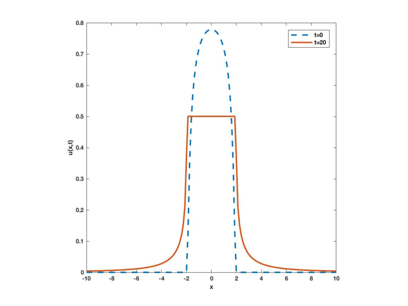
Figure 1. The solution of a fractional Stefan problem with $\varphi(\xi)=\max\{0,\xi-0.5\}$.

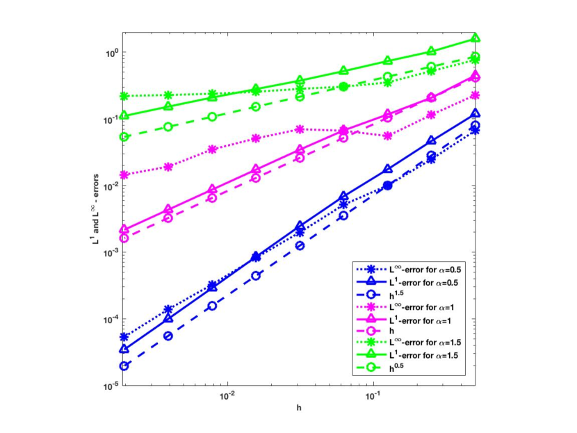
Figure 2. The corresponding $L^{1}$- and $L^{\infty}$-errors using the Midpoint Rule.

4. Proofs of main results

The scheme (2.5) can be seen as an operator splitting method with alternating explicit and implicit steps. The explicit step is given by the operator

($$T^{\textup{exp}} T^{\textup{exp}}[\psi](x):=\psi(x)+\mathcal{L}^{\nu}[\varphi(\psi)](x)\qquad\text{for}\qquad x\in\mathbb{R}^{N},$$)

while the implicit step is given by the operator

($$T^{\textup{imp}} T^{\textup{imp}}[\rho](x):=w(x)\qquad\text{for}\qquad\mathbb{R}^{N},$$)

where $w$ is the solution of the nonlinear elliptic equation

(EP) $$w(x)-\mathcal{L}^{\nu}[\varphi(w)](x)=\rho(x)\qquad\text{in}\qquad\mathbb{R}^{N},$$

We can then write the scheme (2.5) in the following way:

(4.1) $$U_{h}^{j}(x)=T^{\textup{imp}}\Big{[}T^{\textup{exp}}[U_{h}^{j-1}]+\Delta t_{j}F^{j}\Big{]}(x),$$

where we take $\nu=\Delta t_{j}\nu_{2}^{h}$, $\varphi=\varphi_{2}^{h}$ in ($T^{\textup{exp}}$) and $\nu=\Delta t_{j}\nu_{1}^{h}$, $\varphi=\varphi_{1}^{h}$ in ($T^{\textup{imp}}$). To study the properties of the scheme (2.5), we are reduced to study the properties of the operators $T^{\textup{exp}}$ and $T^{\textup{imp}}$.

4.1. Properties of the numerical scheme

In this section we prove Theorems 2.6 and 2.8. We start by analyzing the operators $T^{\textup{exp}}$ and $T^{\textup{imp}}$. By Fubini’s theorem and simple computations, we have the following result.

Lemma 4.1.

1. If (2.1) holds, $p\in\{1,\infty\}$, and $\psi\in L^{p}(\mathbb{R}^{N})$, then $\mathcal{L}^{\nu}[\psi]$ is well-defined in $L^{p}(\mathbb{R}^{N})$ and

   $$\|\mathcal{L}^{\nu}[\psi]\|_{L^{p}(\mathbb{R}^{N})}\leq 2\|\psi\|_{L^{p}(\mathbb{R}^{N})}\nu(\mathbb{R}^{N}).$$

2. If (2.1) holds and $\psi\in L^{1}(\mathbb{R}^{N})$, then $\int_{\mathbb{R}^{N}}\mathcal{L}^{\nu}[\psi]\,\mathrm{d}x=0$.

Hence if (2.1) and ($\textup{A}_{\varphi}$) hold, then $T^{\textup{exp}}$ is a well-defined operator on $L^{\infty}(\mathbb{R}^{N})$, and if $\varphi(\psi)\in L^{1}(\mathbb{R}^{N})$, then $\int T^{\textup{exp}}[\psi]\,\mathrm{d}x=\int\psi\,\mathrm{d}x$. For the operator $T^{\textup{imp}}$ we have the following result:

Theorem 4.2.

Assume (2.1) and ($\textup{A}_{\varphi}$). If $\rho\in L^{1}(\mathbb{R}^{N})\cap L^{\infty}(\mathbb{R}^{N})$, then there exists a unique a.e.-solution $T^{\textup{imp}}[\rho]=w\in L^{1}(\mathbb{R}^{N})\cap L^{\infty}(\mathbb{R}^{N})$ of (EP).

We now list the remaining properties of $T^{\textup{exp}}$ and $T^{\textup{imp}}$ that we use in this section.

Theorem 4.3.

Assume (2.1), $\phi,\hat{\phi}\in L^{1}(\mathbb{R}^{N})\cap L^{\infty}(\mathbb{R}^{N})$, and either

$$\text{\eqref{philipas}\ \ and\ \ $L_{\varphi}\nu(\mathbb{R}^{N})\leq 1$}\ \ \text{for}\ \ T^{\textup{exp}}\quad\qquad\text{or}\quad\qquad\text{\eqref{phias}}\ \ \text{for}\ \ T^{\textup{imp}},$$

where $L_{\varphi}:=\sup_{|\zeta|\leq\max\{\|\phi\|_{L^{\infty}},\|\hat{\phi}\|_{L^{\infty}}\}}|\varphi^{\prime}(\zeta)|$.

Whether $T=T^{\textup{exp}}$ or $T=T^{\textup{imp}}$, it then follows that

1. (Comparison) if $\phi\leq\hat{\phi}$ a.e., then $T[\phi]\leq T[\hat{\phi}]$ a.e.;

2. ($L^{1}$-contraction) $\int_{\mathbb{R}^{N}}(T[\phi](x)-T[\hat{\phi}](x))^{+}\,\mathrm{d}x\leq\int_{\mathbb{R}^{N}}(\phi(x)-\hat{\phi}(x))^{+}\,\mathrm{d}x$;

3. ($L^{1}$-bound) $\|T[\phi]\|_{L^{1}(\mathbb{R}^{N})}\leq\|\phi\|_{L^{1}(\mathbb{R}^{N})}$; and

4. ($L^{\infty}$-bound) $\|T[\phi]\|_{L^{\infty}(\mathbb{R}^{N})}\leq\|\phi\|_{L^{\infty}(\mathbb{R}^{N})}$.

The proofs of Theorems 4.2 and 4.3 will be given in Section 5.

Remark 4.4.

Note that $L_{\varphi}\nu(\mathbb{R}^{N})\leq 1$ is a CFL-condition yielding monotonicity/comparison for the scheme.

We are now ready to prove a priori, $L^{1}$-contraction, existence, and uniqueness results for the numerical scheme (2.5).

Proof of Theorem 2.6.

(a) Note that $U^{0}_{h}\leq V^{0}_{h}$ and $F^{j}\leq G^{j}$. If $U^{j-1}_{h}\leq V^{j-1}_{h},$ then by Theorem 4.3 (a),

$$(T^{\textup{exp}}[U_{h}^{j-1}]+\Delta t_{j}F^{j})-(T^{\textup{exp}}[V_{h}^{j-1}]+\Delta t_{j}G^{j})$$

$$=(T^{\textup{exp}}[U_{h}^{j-1}]-T^{\textup{exp}}[V_{h}^{j-1}])+\Delta t_{j}(F^{j}-G^{j})\leq 0$$

and thus, by (4.1) and Theorem 4.3 (a) again,

$$U^{j}_{h}-V^{j}_{h}=T^{\textup{imp}}\Big{[}T^{\textup{exp}}[U_{h}^{j-1}]+\Delta t_{j}F^{j}\Big{]}-T^{\textup{imp}}\Big{[}T^{\textup{exp}}[V_{h}^{j-1}]+\Delta t_{j}G^{j}\Big{]}\leq 0.$$

Since $U^{0}_{h}-V^{0}_{h}\leq 0$, part (a) follows by induction.

(b)–(c) Let $X$ be either $L^{1}(\mathbb{R}^{d})$ or $L^{\infty}(\mathbb{R}^{d})$. By Theorem 4.3 (c) or (d),

$$\begin{split}\|U_{h}^{j}\|_{X}&=\Big{\|}T^{\textup{imp}}\Big{[}T^{\textup{exp}}[U_{h}^{j-1}]+\Delta t_{j}F^{j}\Big{]}\Big{\|}_{X}\leq\|T^{\textup{exp}}[U_{h}^{j-1}]+\Delta t_{j}F^{j}]\|_{X}\\ &\leq\|U_{h}^{j-1}\|_{X}+\Delta t_{j}\|F^{j}\|_{X}.\end{split}$$

Then we iterate $j$ down to zero to get $\|U_{h}^{j}\|_{X}\leq\|U_{h}^{0}\|_{X}+\sum_{l=1}^{j}\|F^{l}\|_{X}\Delta t_{l}$, and by the definition of $F^{l}$,

$$\begin{split}&\sum_{l=1}^{j}\|F^{l}\|_{X}\Delta t_{l}=\sum_{l=1}^{j}\bigg{\|}\frac{1}{\Delta t_{l}}\int_{t_{l-1}}^{t_{l}}f(x,\tau)\,\mathrm{d}\tau\bigg{\|}_{X}\Delta t_{l}\leq\int_{0}^{t_{j}}\|f(\cdot,\tau)\|_{X}\,\mathrm{d}\tau.\end{split}$$

(d) Since $\varphi^{h}_{i}$ is locally Lipschitz, now $\varphi^{h}_{i}(U_{h}^{j}),\varphi^{h}_{i}(V_{h}^{j})\in L^{1}$. The result then follows from integrating (2.5) in $x$, iterating $j$ down to zero, and using that the integral of nonsingular Lévy operators acting on integrable functions is zero (Lemma 4.1 (b)). This completes the proof. ∎

Proof of Theorem 2.8.

By two applications of Theorem 4.3 (b),

$$\begin{split}&\int_{\mathbb{R}^{N}}(U_{h}^{j}-V_{h}^{j})^{+}(x)\,\mathrm{d}x\leq\int_{\mathbb{R}^{N}}(U_{h}^{j-1}-V_{h}^{j-1})^{+}(x)\,\mathrm{d}x+\Delta t_{j}\int_{\mathbb{R}^{N}}(F^{j}-G^{j})^{+}(x)\,\mathrm{d}x.\end{split}$$

Then we iterate $j$ down to zero to get

$$\begin{split}&\int_{\mathbb{R}^{N}}(U_{h}^{j}-V_{h}^{j})^{+}(x)\,\mathrm{d}x\leq\int_{\mathbb{R}^{N}}(U_{h}^{0}-V_{h}^{0})^{+}(x)\,\mathrm{d}x+\sum_{l=1}^{j}\Delta t_{l}\int_{\mathbb{R}^{N}}(F^{l}-G^{l})^{+}(x)\,\mathrm{d}x.\end{split}$$

By the definition of $F^{l}$ and $G^{l}$, Jensen’s inequality, and Tonelli’s theorem,

$$\begin{split}\sum_{l=1}^{j}\Delta t_{l}\int_{\mathbb{R}^{N}}(F^{l}-G^{l})^{+}(x)\,\mathrm{d}x&=\sum_{l=1}^{j}\Delta t_{l}\int_{\mathbb{R}^{N}}\bigg{(}\frac{1}{\Delta t_{l}}\int_{t_{l-1}}^{t_{l}}\big{(}f-g\big{)}(x,\tau)\,\mathrm{d}\tau\bigg{)}^{+}\,\mathrm{d}x\\ &\leq\int_{0}^{t_{j}}\int_{\mathbb{R}^{N}}\big{(}f(x,s)-g(x,s)\big{)}^{+}\,\mathrm{d}x\,\mathrm{d}s.\end{split}$$

The proof is complete. ∎

We finish by proving existence of a unique solution of the numerical scheme.

Proof of Theorem 2.4.

Proof by induction. Assume solutions $U_{h}^{i}\in L^{1}\cap L^{\infty}$ of (2.5) exists for $i=1,\dots,j-1$. Then since $\rho=T^{\textup{exp}}[U_{h}^{j-1}]+\Delta t_{j}F^{j}\in L^{1}\cap L^{\infty}$ by Theorem 4.3 and ($\textup{A}_{f}$), existence and uniqueness of an a.e.-solution $T^{\textup{imp}}[\rho]=U_{h}^{j}\in L^{1}\cap L^{\infty}$ of (EP) follows by Theorem 4.2. In view of (4.1), this $U_{h}^{j}$ is the unique a.e.-solution of (2.5) at $t=t_{j}$. ∎

The strategy for the remaining proofs is the following. We first prove equiboundedness and equicontinuity results for the sequence of interpolated solutions $\{\widetilde{U}_{h}\}_{h>0}$ of the scheme (2.5) as $h\to 0^{+}$. By Arzelà-Ascoli and Kolmogorov-Riesz type compactness results, see e.g. the Appendix of [41], we conclude that there is a convergent subsequence in $C([0,T],L^{1}_{\mathrm{loc}}(\mathbb{R}^{N}))$. We use consistency to prove that any such limit must be the unique solution of (1.1). Finally, by a standard argument combining compactness and uniqueness of limit points, we conclude that the full sequence must converge.

4.2. Equicontinuity and compactness of the numerical scheme

In this section we prove Theorem 2.10, equicontinuity in space, and compactness for the scheme. Since $\widetilde{U}_{h}$ is the interpolation of $U_{h}$ defined in (2.11), we will prove the equiboundedness and -continuity first for $U_{h}^{j}$ and then transfer these results to $\widetilde{U}_{h}$. The equiboundedness is a direct corollary of Theorem 2.6 (c).

Lemma 4.5 (Equicontinuity in space).

Assume ($\textup{A}_{u_{0}}$), ($\textup{A}_{f}$), and ($\textup{A}_{\textup{NS}}$) hold for all $h>0$, and let $\{U_{h}^{j}\}_{h>0}$ be a.e.-solutions of (2.5). Then, for all $j\in\mathbb{J}$, all compact sets $K\subset\mathbb{R}^{N}$, and all $\eta>0$,

$$\begin{split}&\sup_{|\xi|\leq\eta}\|U_{h}^{j}-U_{h}^{j}(\cdot+\xi)\|_{L^{1}(K)}\leq\lambda_{u_{0},f}(\eta),\end{split}$$

where $\lambda_{u_{0},f}$ is defined in (2.7).

Proof.

By translation invariance and uniqueness, $U_{h}^{j}(x+\xi)$ is a solution of (2.5) with data $u_{0}(\cdot+\xi)$ and $f(\cdot+\xi,\cdot)$. Taking $V_{h}^{j}(x)=U_{h}^{j}(x+\xi)$ in the $L^{1}$-contraction Theorem 2.8 then concludes the estimate. Continuity of the $L^{1}$-translation and assumptions ($\textup{A}_{u_{0}}$) and ($\textup{A}_{f}$) shows that $\lim_{\eta\to 0}\lambda_{u_{0},f}(\eta)=0$. ∎

Under the additional assumption of having a consistent numerical scheme,

(4.2) $$\sup_{h\in(0,1)}\|\varphi_{i}^{h}(U_{h}^{j})\|_{L^{\infty}(\mathbb{R}^{N})}<\infty$$

and

$$\sup_{h\in(0,1)}\|\mathcal{L}_{i}^{h}[\psi]\|_{L^{1}(\mathbb{R}^{N})}<\infty\qquad\textup{for all}\qquad\psi\in C_{\textup{c}}^{\infty}(\mathbb{R}^{N})$$

for $i=1,2$. The first bound is trivial, while the second follows since $\|\mathcal{L}_{i}^{h}[\psi]\|_{L^{1}(\mathbb{R}^{N})}\leq\|\mathcal{L}_{i}^{h}[\psi]-\mathfrak{L}^{\sigma,\mu}_{i}[\psi]\|_{L^{1}(\mathbb{R}^{N})}+\|\mathfrak{L}^{\sigma,\mu}_{i}[\psi]\|_{L^{1}(\mathbb{R}^{N})}$ is bounded for $h\leq 1$ by Definition 2.2 (ii). These facts allow us to prove the time equicontinuity result Theorem 2.10.

Proof of Theorem 2.10.

We exploit the idea, which is sometimes referred to as the Kružkov interpolation lemma [60], that an estimate on the $L^{1}$-translations in space will give an estimate on the $L^{1}$-translations in time. To simplify, we start by considering right-hand sides $f=0$.

The numerical scheme (2.5) can be written as

$$U_{h}^{j}(x)-U_{h}^{j-1}(x)=\Delta t_{j}\left(\mathcal{L}^{h}_{1}[\varphi_{1}^{h}(U_{h}^{j})](x)+\mathcal{L}^{h}_{2}[\varphi_{2}^{h}(U_{h}^{j-1})](x)\right).$$

Let $\omega_{\delta}$ be a standard mollifier in $\mathbb{R}^{N}$ obtained by scaling from a fixed $\omega$, and define $(U_{h}^{j})_{\delta}(x):=(U_{h}^{j}*\omega_{\delta})(x)$. Taking the convolution of the scheme with $\omega_{\delta}$ and using the fact that the operator $\mathcal{L}^{\nu}$ commutes with convolutions, we find that

$$\begin{split}(U_{h}^{j})_{\delta}(x)-(U_{h}^{j-1})_{\delta}(x)&=\Delta t_{j}\left(\mathcal{L}^{h}_{1}[\varphi_{1}^{h}(U_{h}^{j})]+\mathcal{L}^{h}_{2}[\varphi_{2}^{h}(U_{h}^{j-1})]\right)\ast\omega_{\delta}(x)\\ &=\Delta t_{j}\left(\varphi_{1}^{h}(U_{h}^{j})\ast\mathcal{L}^{h}_{1}[\omega_{\delta}](x)+\varphi_{2}^{h}(U_{h}^{j-1})\ast\mathcal{L}^{h}_{2}[\omega_{\delta}](x)\right).\end{split}$$

We integrate over any compact set $K\subset\mathbb{R}^{N}$, use Theorem 2.6 (c), and (4.2), and standard properties of mollifiers (see e.g. the proof of Lemma 4.3 in [33]), to get

(4.3) $$\begin{split}&\int_{K}\big{|}(U_{h}^{j})_{\delta}-(U_{h}^{j-1})_{\delta}\big{|}\,\mathrm{d}x\\ &\leq\Delta t_{j}|K|\Big{(}\|\varphi_{1}^{h}(U_{h}^{j})\|_{L^{\infty}}\|\mathcal{L}^{h}_{1}[\omega_{\delta}]\|_{L^{1}}+\|\varphi_{2}^{h}(U_{h}^{j-1})\|_{L^{\infty}}\|\mathcal{L}^{h}_{2}[\omega_{\delta}]\|_{L^{1}}\Big{)}\\ &\leq\Delta t_{j}|K|\Bigg{(}\sup_{|r|\leq M_{u_{0},f}}\!\!|\varphi_{1}^{h}(r)|\,\|\mathcal{L}^{h}_{1}[\omega_{\delta}]\|_{L^{1}}+\sup_{|r|\leq M_{u_{0},f}}\!\!|\varphi_{2}^{h}(r)|\,\|\mathcal{L}^{h}_{2}[\omega_{\delta}]\|_{L^{1}}\Bigg{)}\\ &\leq C_{K}\Delta t_{j}(1+\delta^{-2}),\end{split}$$

where $C_{K}=C_{K,u_{0},f,\varphi_{1},\varphi_{2},\nu_{1},\nu_{2}}$ is given by (2.10) with constant $c$ such that $c(1+\delta^{-2})$ is a uniform in $h$ upper bound on $\max_{i=1,2}\|\mathcal{L}^{h}_{i}[\omega_{\delta}]\|_{L^{1}}$. This upper bound follows from (2.1), the uniform Lévy condition ($\textup{A}_{\nu^{h}}$), and the properties of $\omega_{\delta}$:

$$\begin{split}\|\mathcal{L}^{h}_{i}[\omega_{\delta}]\|_{L^{1}}&\leq C\|D^{2}\omega_{\delta}\|_{L^{1}}\Big{(}\int_{|z|\leq 1}|z|^{2}\,\mathrm{d}\nu^{h}_{i}(z)\Big{)}+2\|\omega_{\delta}\|_{L^{1}}\int_{|z|>1}\,\mathrm{d}\nu^{h}_{i}(z)\\ &\leq\delta^{-2}C\|D^{2}\omega\|_{L^{1}}\Big{(}\int_{|z|\leq 1}|z|^{2}\,\mathrm{d}\nu^{h}_{i}(z)\Big{)}+2\|\omega\|_{L^{1}}\int_{|z|>1}\,\mathrm{d}\nu^{h}_{i}(z).\end{split}$$

By iterating (4.3) and using Tonelli plus Theorem 2.8, we obtain

$$\begin{split}\|U_{h}^{j}-U_{h}^{j-k}\|_{L^{1}(K)}&\leq\|U_{h}^{j}-(U_{h}^{j})_{\delta}\|_{L^{1}(K)}+\|(U_{h}^{j})_{\delta}-(U_{h}^{j-k})_{\delta}\|_{L^{1}(K)}\\ &\quad+\|(U_{h}^{j-k})_{\delta}-U_{h}^{j-k}\|_{L^{1}(K)}\\ &\leq 2\sup_{|h|\leq\delta}\|u_{0}-u_{0}(\cdot+h)\|_{L^{1}(\mathbb{R}^{N})}+C_{K}(t_{j}-t_{j-k})(1+\delta^{-2}),\end{split}$$

Now we conclude by taking $\delta=(t_{j}-t_{j-k})^{\frac{1}{3}}$.

The proof for $f\not\equiv 0$ follows in a similar way after using that

(4.4) $$\sum_{l=j-k+1}^{j}\|F^{l}\|_{L^{\infty}(\mathbb{R}^{N})}\Delta t_{l}\leq\int_{t_{j-k}}^{t_{j}}\|f(\cdot,\tau)\|_{L^{\infty}(\mathbb{R}^{N})}\,\mathrm{d}\tau$$

for $F^{l}$ defined as in (2.4). ∎

The equiboundedness, Lemma 4.5, and Theorem 2.10 (plus Theorems 2.6 and 2.8) immediately transfers, mutatis mutandis, to $\widetilde{U}_{h}$. We only restate the (slightly modified) equicontinuity in time result for $\widetilde{U}_{h}$ here:

Lemma 4.6 (Equicontinuity in time).

Assume ($\textup{A}_{f}$), ($\textup{A}_{u_{0}}$), $\Delta t=o_{h}(1)$, and for all $h>0$, let $U^{j}_{h}$ be the solution of a consistent scheme (2.5) satisfying ($\textup{A}_{\textup{NS}}$) and ($\textup{A}_{\nu^{h}}$). Then, for $t,s\in[0,T]$,

(4.5) $$\begin{split}\|\widetilde{U}_{h}(\cdot,t)-\widetilde{U}_{h}(\cdot,s)\|_{L^{1}(K)}&\leq\Lambda_{K}(|t-s|)\\ &\quad+|K|\Big{(}\int_{s}^{t}\|f(\cdot,\tau)\|_{L^{\infty}(\mathbb{R}^{N})}\,\mathrm{d}\tau+\lambda(|t-s|,\Delta t)\Big{)},\end{split}$$

where $\lambda$ is continuous and satisfies

(4.6) $$\sup_{\Delta t\leq 1}|\lambda(\delta,\Delta t)|\stackrel{{\scriptstyle\delta\to 0}}{{\longrightarrow}}0,\quad\text{and for $\delta\in[0,T]$,}\quad\lambda(\delta,\Delta t)\stackrel{{\scriptstyle\Delta t\to 0}}{{\longrightarrow}}0.$$

Proof.

1) Assume $f=0$. The proof of (4.5) is like the proof of Theorem 2.10 with a slightly modified end where the time interpolant (2.11) appears: For $t\in(t_{j-1},t_{j}]$ and $s\in(t_{j-k-1},t_{j-k}]$,

$$\begin{split}\|(\widetilde{U}_{h})_{\delta}(\cdot,t)-(\widetilde{U}_{h})_{\delta}(\cdot,s)\|_{L^{1}}&\leq\big{\|}(\widetilde{U}_{h})_{\delta}(\cdot,t)-(U_{h}^{j-1})_{\delta}\|_{L^{1}}+\|(U_{h}^{j-k})_{\delta}-(\widetilde{U}_{h})_{\delta}(\cdot,s)\|_{L^{1}}.\\ &\quad+\sum_{l=j-k+1}^{j-1}\|(U^{l}_{h})_{\delta}-(U^{l-1}_{h})_{\delta}\|_{L^{1}}\end{split}$$

Since by the definition of linear interpolation,

$$\big{\|}(\widetilde{U}_{h})_{\delta}(\cdot,t)-(U^{j-1}_{h})_{\delta}\|_{L^{1}}\leq\frac{t-t_{j-1}}{\Delta t_{j}}\big{\|}(U^{j}_{h})_{\delta}-(U^{j-1}_{h})_{\delta}\big{\|}_{L^{1}},$$

$$\|(U^{j-k}_{h})_{\delta}-(\widetilde{U}_{h})_{\delta}(\cdot,s)\|_{L^{1}}\leq\frac{t_{j-k}-s}{\Delta t_{j-k}}\big{\|}(U^{j-k}_{h})_{\delta}-(U^{j-k-1}_{h})_{\delta}\big{\|}_{L^{1}},$$

it follows by repeated use of (4.3) that

$$\|(\widetilde{U}_{h})_{\delta}(\cdot,t)-(\widetilde{U}_{h})_{\delta}(\cdot,s)\|_{L^{1}} \leq\Big{(}(t-t_{j-1})+\sum_{l=j-k+1}^{j-1}\Delta t_{l}+(t_{j-k}-s)\Big{)}C_{K}(1+\delta^{-2})$$

$$=(t-s)C_{K}(1+\delta^{-2}).$$

At this point we can conlclude the proof as before when $f=0$.

2) Assume $f\not\equiv 0$. From the proof of Theorem 2.10 with $f\not\equiv 0$ and an inequality as (4.4), we find that

$$\begin{split}\lambda(|t-s|,\Delta t):=\int_{s}^{t}\big{(}\hat{F}_{\Delta t}(\tau)-\|f(\cdot,\tau)\|_{L^{\infty}(\mathbb{R}^{N})}\big{)}\,\mathrm{d}\tau,\end{split}$$

where the piecewise constant function $\hat{F}_{\Delta t}$ is defined from $\tau\mapsto\|f(\cdot,\tau)\|_{L^{\infty}(\mathbb{R}^{N})}$ by averages:

$$\hat{F}_{\Delta t}(\tau):=\frac{1}{\Delta t_{l}}\int_{t_{l-1}}^{t_{l}}\|f(\cdot,\tau^{\prime})\|_{L^{\infty}(\mathbb{R}^{N})}\,\mathrm{d}\tau^{\prime}\qquad\text{for}\qquad\tau\in(t_{l-1},t_{l}],\quad l\in\mathbb{J}.$$

A standard argument shows that $\hat{F}_{\Delta t}\to\|f(\cdot,\tau)\|_{L^{\infty}(\mathbb{R}^{N})}$ in $L^{1}(0,T)$ as $\Delta t\to 0^{+}$, and then the sequence $\{\hat{F}_{\Delta t}-\|f(\cdot,\tau)\|_{L^{\infty}(\mathbb{R}^{N})}\}_{\Delta t\leq 1}$ is equi-integrable by the Vitalli convergence theorem. Since equi-integrability implies that

$$\lim_{|t-s|\to 0}\sup_{\Delta t\leq 1}\int_{[s,t]}\big{|}\hat{F}_{\Delta t}(\tau)-\|f(\cdot,\tau)\|_{L^{\infty}(\mathbb{R}^{N})}\big{|}\,\mathrm{d}\tau=0,$$

the two claims in (4.6) readily follows. ∎

In view of equiboundedness and -continuity of $\{\widetilde{U}_{h}\}_{h>0}$, we can now use the Arzelà-Ascoli and Kolmogorov-Riesz type compactness results, see e.g. the Appendix of [41], to conclude the following result:

Theorem 4.7 (Compactness).

Assume ($\textup{A}_{f}$), ($\textup{A}_{u_{0}}$), $\Delta t=o_{h}(1)$, (2.5) is a consistent scheme satisfying ($\textup{A}_{\nu^{h}}$) and such that ($\textup{A}_{\textup{NS}}$) holds for every $h>0$, let $\{U_{h}^{j}\}_{h>0}$ be the solutions of (2.5) and $\{\widetilde{U}_{h}\}_{h>0}$ their time interpolants defined in (2.11). Then there exists a subsequence $\{\widetilde{U}_{h_{n}}\}_{n\in\mathbb{N}}$ and a $u\in C([0,T];L_{\textup{loc}}^{1}(\mathbb{R}^{N}))$ such that

$$\widetilde{U}_{h_{n}}\to u\qquad\text{in}\qquad C([0,T];L_{\textup{loc}}^{1}(\mathbb{R}^{N}))\quad\text{and\quad a.e.}\qquad\text{as}\qquad n\to\infty.$$

4.3. Convergence of the numerical scheme

In this section we prove convergence of the scheme, Theorem 2.11. We start with a consequence of the consistency and stability of the scheme and the stability of the equation.

Lemma 4.8.

Under the assumptions of Theorem 4.7, any subsequence of $\{\widetilde{U}_{h}\}_{h>0}$ that converges in $C([0,T];L_{\textup{loc}}^{1}(\mathbb{R}^{N}))$, converges to a distributional solution $u\in L^{1}(Q_{T})\cap L^{\infty}(Q_{T})$ of (1.1).

An immediate corollary of this lemma, the compactness in Theorem 4.7, and uniqueness in Theorem 2.2, is then the following result.

Corollary 4.9.

Under the assumptions of Theorem 4.7, any subsequence of $\{\widetilde{U}_{h}\}_{h>0}$ has a further subsequence that converges in $C([0,T];L_{\textup{loc}}^{1}(\mathbb{R}^{N}))$ to the unique distributional solution $u\in L^{1}(Q_{T})\cap L^{\infty}(Q_{T})$ of (1.1).

We now prove convergence of the scheme, Theorem 2.11.

Proof of Theorem 2.11.

By compactness, Theorem 4.7, there is a subsequence of $\{\widetilde{U}_{h}\}_{h>0}$ that converge to some function $u$ in $C([0,T];L_{\textup{loc}}^{1}(\mathbb{R}^{N}))$. By Lemma 4.8, $u$ is a distributional solution of (1.1) belonging to $L^{1}(Q_{T})\cap L^{\infty}(Q_{T})$. Then the whole sequence converges since it is bounded and other limit points are excluded by Corollary 4.9. ∎

It remains to prove Lemma 4.8.

Proof of Lemma 4.8.

Take any $C([0,T];L_{\textup{loc}}^{1}(\mathbb{R}^{N}))$ converging subsequence of $\{\widetilde{U}_{h}\}_{h>0}$ and let $u$ be its limit. For simplicity we also denote the subsequence by $\{\widetilde{U}_{h}\}_{h>0}$. Remember that $\widetilde{U}_{h}$ is the time interpolation of $U_{h}$ defined in (2.11).

1) The limit $u\in L^{1}(Q_{T})\cap L^{\infty}(Q_{T})$. There is a further subsequence converging to $u$ for all $t$ and a.e. $x$. Hence we find that the $L^{\infty}$ bound of Theorem 2.6 (c) is inherited by $u$. Similarly, by Fatou’s lemma, also the $L^{1}$ bound of Theorem 2.6 (b) carries over to $u$. Hence we can conclude that $u\in L^{1}(Q_{T})\cap L^{\infty}(Q_{T})$.

We proceed to prove that $u$ is a distributional solution of (1.1), see Definition 2.1.

2) Weak formulation of the numerical scheme (2.5). Let $\psi\in C_{\textup{c}}^{\infty}(\mathbb{R}^{N}\times[0,T))$. We multiply the scheme (2.5) by $\psi(x,t_{j-1})\Delta t_{j}$, integrate in space, sum in time, and use the self-adjointness of $\mathcal{L}^{h}_{1},\mathcal{L}^{h}_{2}$, to get

(4.7) $$\begin{split}\int_{\mathbb{R}^{N}}\sum_{j=1}^{J}&\frac{U_{h}^{j}-U_{h}^{j-1}}{\Delta t_{j}}\psi(x,t_{j-1})\Delta t_{j}\,\mathrm{d}x=\int_{\mathbb{R}^{N}}\sum_{j=1}^{J}\varphi_{1}^{h}(U_{h}^{j})\mathcal{L}^{h}_{1}[\psi(\cdot,t_{j-1})]\Delta t_{j}\,\mathrm{d}x\\ \quad&+\int_{\mathbb{R}^{N}}\sum_{j=1}^{J}\varphi_{2}^{h}(U_{h}^{j-1})\mathcal{L}^{h}_{2}[\psi(\cdot,t_{j-1})]\Delta t_{j}\,\mathrm{d}x+\int_{\mathbb{R}^{N}}\sum_{j=1}^{J}F^{j}(x)\psi(x,t_{j-1})\Delta t_{j}\,\mathrm{d}x.\end{split}$$

In the rest of the proof we will show that the different terms in this equation converge to the corresponding terms in (2.2) and thereby conclude the proof.

3) Convergence to the time derivative. By summation by parts, $U_{h}^{0}=u_{0}$, and $\psi(x,t_{J-1})=0$ for $\Delta t$ small enough since $\psi$ has compact support,

$$\begin{split}&\int_{\mathbb{R}^{N}}\sum_{j=1}^{J}\frac{U_{h}^{j}(x)-U_{h}^{j-1}(x)}{\Delta t_{j}}\psi(x,t_{j-1})\Delta t_{j}\,\mathrm{d}x\\ &=-\int_{\mathbb{R}^{N}}\sum_{j=1}^{J-1}U_{h}^{j}(x)\frac{\psi(x,t_{j})-\psi(x,t_{j-1})}{\Delta t_{j}}\Delta t_{j}\,\mathrm{d}x\\ &\quad+\int_{\mathbb{R}^{N}}U_{h}^{J}(x)\psi(x,t_{J-1})\,\mathrm{d}x-\int_{\mathbb{R}^{N}}U_{h}^{0}(x)\psi(x,0)\,\mathrm{d}x\\ &=-I+0-\int_{\mathbb{R}^{N}}u_{0}(x)\psi(x,0)\,\mathrm{d}x.\end{split}$$

To continue, we note that for any $r>0$,

$$\sum_{j=1}^{J-1}\frac{\psi(x,t_{j})-\psi(x,t_{j-1})}{\Delta t_{j}}\mathbf{1}_{[t_{j-1},t_{j})}(t)\to\partial_{t}\psi(x,t)\quad\text{in}\quad L^{\infty}(\mathbb{R}^{N}\times[0,T-r))$$

as $\Delta t\to 0^{+}$. Then since $U_{h}$ is uniformly bounded and $\widetilde{U}_{h}$ converges to $u$ in $C(0,T;L_{\textup{loc}}^{1}(\mathbb{R}^{N}))$, and $\psi$ has compact support, a standard argument shows that

$$I=\int_{\mathbb{R}^{N}}\sum_{j=1}^{J-1}U_{h}^{j}(x)\frac{\psi(x,t_{j})-\psi(x,t_{j-1})}{\Delta t_{j}}\Delta t_{j}\,\mathrm{d}x\to\int_{\mathbb{R}^{N}}\int_{0}^{T}u(x,t)\partial_{t}\psi(x,t)\,\mathrm{d}t\,\mathrm{d}x$$

as $h\to 0^{+}$. Combining all estimates, we conclude that as $h\to 0^{+}$,

$$\int_{\mathbb{R}^{N}}\sum_{j=1}^{J}\frac{U_{h}^{j}-U_{h}^{j-1}}{\Delta t_{j}}\psi(x,t_{j-1})\Delta t_{j}\,\mathrm{d}x$$

$$\to-\int_{\mathbb{R}^{N}}\int_{0}^{T}u\,\partial_{t}\psi\,\mathrm{d}t\,\mathrm{d}x-\int_{\mathbb{R}^{N}}u_{0}(x)\psi(x,0)\,\mathrm{d}x.$$

4) Convergence of the nonlocal terms. We start by the $\mathcal{L}^{h}_{1}$-term. By adding and subtracting terms we find that

$$\int_{\mathbb{R}^{N}}\sum_{j=1}^{J}\varphi_{1}^{h}(U_{h}^{j})\mathcal{L}^{h}_{1}[\psi(\cdot,t_{j-1})]\Delta t_{j}\,\mathrm{d}x= \int_{0}^{T}\int_{\mathbb{R}^{N}}\varphi_{1}(u)\mathfrak{L}^{\sigma,\mu}_{1}[\psi(\cdot,t)]\,\mathrm{d}t\,\mathrm{d}x$$

$$+E_{1}+E_{2}+E_{3}+E_{4},$$

where

$$|E_{1}|\leq\int_{\mathbb{R}^{N}}\sum_{j=1}^{J}\int_{t_{j-1}}^{t_{j}}|\varphi_{1}^{h}(U_{h}^{j})|\big{|}\mathcal{L}^{h}_{1}[\psi(\cdot,t_{j-1})]-\mathfrak{L}^{\sigma,\mu}_{1}[\psi(\cdot,t_{j-1})]\big{|}\,\mathrm{d}t\,\mathrm{d}x$$

$$|E_{2}|\leq\int_{\mathbb{R}^{N}}\sum_{j=1}^{J}\int_{t_{j-1}}^{t_{j}}|\varphi_{1}^{h}(U_{h}^{j})|\big{|}\mathfrak{L}^{\sigma,\mu}_{1}[\psi(\cdot,t_{j-1})]-\mathfrak{L}^{\sigma,\mu}_{1}[\psi(\cdot,t)]\big{|}\,\mathrm{d}t\,\mathrm{d}x$$

$$|E_{3}|\leq\int_{\mathbb{R}^{N}}\sum_{j=1}^{J}\int_{t_{j-1}}^{t_{j}}\big{|}\varphi_{1}^{h}(U_{h}^{j})-\varphi_{1}(U_{h}^{j})\big{|}|\mathfrak{L}^{\sigma,\mu}_{1}[\psi(\cdot,t)]|\,\mathrm{d}t\,\mathrm{d}x$$

$$|E_{4}|\leq\int_{\mathbb{R}^{N}}\sum_{j=1}^{J}\int_{t_{j-1}}^{t_{j}}\big{|}\varphi_{1}(U_{h}^{j}(x))-\varphi_{1}(u(x,t))\big{|}|\mathfrak{L}^{\sigma,\mu}_{1}[\psi(\cdot,t)]|\,\mathrm{d}t\,\mathrm{d}x.$$

First note that by (2.1) and Remark 2.1 (b),

$$\sup_{t\in[0,T]}\|\mathfrak{L}^{\sigma,\mu}_{1}[\psi(\cdot,t)]\|_{L^{1}}\leq C\sup_{t\in[0,T]}(\|D^{2}\psi(\cdot,t)\|_{L^{1}}+\|\psi(\cdot,t)\|_{L^{1}})=:K<\infty.$$

Then by consistency (Definition 2.2 (ii)),

$$\sup_{t\in[0,T]}\|(\mathfrak{L}^{\sigma,\mu}_{1}-\mathcal{L}^{h}_{1})[\psi(\cdot,t)]\|_{L^{1}(\mathbb{R}^{N})}\leq\sup_{t\in[0,T]}\|\psi(\cdot,t)\|_{W^{k_{1},1}(\mathbb{R}^{N})}o_{h}(1)\stackrel{{\scriptstyle h\to 0^{+}}}{{\longrightarrow}}0.$$

By the uniform boundedness of $U_{h}$ (Theorem 2.6 (c)) continuity of $\varphi$ ($\textup{A}_{\varphi}$), it first follows that $\|\varphi_{1}(U_{h}^{j})\|_{L^{\infty}(Q_{T})}\leq C$, and then by the uniform convergence of $\varphi_{1}^{h}\to\varphi_{1}$ (Definition 2.2 (iii)) and taking $h$ small enough,

$$\|\varphi_{1}^{h}(U_{h}^{j})-\varphi_{1}(U_{h}^{j})\|_{L^{\infty}(Q_{T})}\stackrel{{\scriptstyle h\to 0^{+}}}{{\longrightarrow}}0\quad\text{and}\quad\|\varphi_{1}^{h}(U_{h}^{j})\|_{L^{\infty}(Q_{T})}\leq 2C.$$

From these considerations we can immediately conclude that $E_{1},E_{3}\to 0$ as $h\to 0^{+}$.

To see that $E_{2}\to 0$, we now only need to observe that by linearity of $\mathfrak{L}^{\sigma,\mu}$ and a Taylor expansion,

$$\|\mathfrak{L}^{\sigma,\mu}_{1}[\psi(\cdot,t_{j-1})]-\mathfrak{L}^{\sigma,\mu}_{1}[\psi(\cdot,t)]\|_{L^{1}}\leq\Delta t\sup_{s\in[0,T]}\|\mathfrak{L}^{\sigma,\mu}_{1}[\partial_{t}\psi(\cdot,s)]|_{L^{1}},$$

and that $\|\mathfrak{L}^{\sigma,\mu}_{1}[\partial_{t}\psi(\cdot,s)]|_{L^{1}}\leq C\sup_{s\in[0,T]}\big{(}\|D^{2}\partial_{t}\psi(\cdot,s))\|_{L^{1}}+\|\partial_{t}\psi(\cdot,s)\|_{L^{1}}\big{)}<\infty$. Finally, we see that $E_{4}\to 0$ by the dominated convergence theorem since $\varphi_{1}(\widetilde{U}_{h})$ is uniformly bounded and we may assume (by taking a further subsequence if necessary) $\widetilde{U}_{h}\to u$ a.e. and hence $\varphi_{1}(\widetilde{U}_{h})\to\varphi_{1}(u)$ a.e. in $Q_{T}$ as $h\to 0^{+}$ by ($\textup{A}_{\varphi}$).

A similar argument shows the convergence of the $\mathcal{L}^{h}_{2}$-term, and we can therefore conclude that as $h\to 0^{+}$,

$$\begin{split}&\int_{\mathbb{R}^{N}}\sum_{j=1}^{J}\varphi_{1}^{h}(U_{h}^{j})\mathcal{L}^{h}_{1}[\psi(\cdot,t_{j-1})]\Delta t_{j}\,\mathrm{d}x+\int_{\mathbb{R}^{N}}\sum_{j=1}^{J}\varphi_{2}^{h}(U_{h}^{j-1})\mathcal{L}^{h}_{2}[\psi(\cdot,t_{j-1})]\Delta t_{j}\,\mathrm{d}x\\ &\to\int_{\mathbb{R}^{N}}\int_{0}^{T}\varphi_{1}(u)\mathfrak{L}^{\sigma,\mu}_{1}[\psi(\cdot,t)]\,\mathrm{d}t\,\mathrm{d}x+\int_{\mathbb{R}^{N}}\int_{0}^{T}\varphi_{2}(u)\mathfrak{L}^{\sigma,\mu}_{2}[\psi(\cdot,t)]\,\mathrm{d}t\,\mathrm{d}x.\end{split}$$

5) Convergence to the right-hand side. By the definition of $F^{j}$,

$$\bigg{|}\int_{\mathbb{R}^{N}}\bigg{(}\sum_{j=1}^{J}F^{j}(x)\psi(x,t_{j-1})\Delta t_{j}-\int_{0}^{T}f(x,t)\psi(x,t)\,\mathrm{d}t\bigg{)}\,\mathrm{d}x\bigg{|}$$

$$\leq\int_{\mathbb{R}^{N}}\sum_{j=1}^{J}\int_{t_{j-1}}^{t_{j}}|\psi(x,t)-\psi(x,t_{j-1})||f(x,t)|\,\mathrm{d}t\,\mathrm{d}x$$

$$\leq\|\partial_{t}\psi\|_{L^{\infty}(Q_{T})}\|f\|_{L^{1}(Q_{T})}\Delta t\to 0^{+}\qquad\text{as}\qquad h\to 0^{+}.$$

6) Conclusion. In view of steps 3) – 5) and Definition 2.2 (i), if we pass to the limit as $h\to 0^{+}$ in (4.7), we find that $u$ satisfy (2.2). In view of step 1), $u$ is then a distributional solution of (1.1) according to Definition 2.1.

∎

4.4. Numerical schemes on uniform spatial grids

Proof of Proposition 2.13.

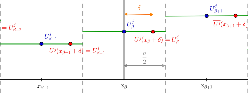
Figure 3. The relation between $U_{\beta}^{j}$ and $\overline{U^{j}}$ in Proposition 2.13.

See Figure 3 for the relation between $U_{\beta}^{j}$ and $\overline{U^{j}}$.

(a) Let $x_{\beta}\in\mathcal{G}_{h}$. Since the scheme (2.5) is translation invariant in $x$, it follows that $U^{j}$ and $U^{j}(\cdot+y)$ are solutions of (2.5) with $\overline{U^{0}},\overline{F^{j}}$ and $\overline{U^{0}}(\cdot+y),\overline{F^{j}}(\cdot+y)$ as data respectively. By uniqueness (Theorem 2.4) and the fact that $\overline{U^{0}}(x_{\beta})=U_{\beta}^{0}=\overline{U^{0}}(x_{\beta}+y)$ and $\overline{F^{j}}(x_{\beta})=F_{\beta}^{j}=\overline{F^{j}}(x_{\beta}+y)$ for all $y\in R_{h}$ and $j>0$, we get that $U^{j}$ is constant on $x_{\beta}+R_{h}$ (a.e.) for all $j>0$. Take a piecewise constant version of $U^{j}$ and let $U_{\beta}^{j}:=h^{-N}\int_{x_{\beta}+R_{h}}U^{j}(x)\,\mathrm{d}x=U^{j}(x)$ for all $x\in x_{\beta}+R_{h}$. In particular, $U^{j}(x_{\beta})=U_{\beta}^{j}$.

Now, let $y\in x_{\beta}+R_{h}$ be such that the scheme (2.5) holds at $y$. Since the grid $\mathcal{G}_{h}$ is uniform and $\mathcal{S}_{1},\mathcal{S}_{2}\subset\mathcal{G}_{h}$, $U^{j}(y+z_{\beta})=U_{\beta+\gamma}^{j}$ for any $z_{\gamma}\in\mathcal{G}_{h}$ and any $j$, and then

$$\mathcal{L}_{i}^{h}[\varphi_{i}^{h}(U^{j})](y) =\sum_{\beta\not=0}\big{(}\varphi_{i}^{h}(U^{j}(y+z_{\beta}))-\varphi_{i}^{h}(U^{j}(y))\big{)}\omega_{\beta,h}$$

$$=\sum_{\beta\not=0}\big{(}\varphi_{i}^{h}(U_{\beta+\gamma}^{j})-\varphi_{i}^{h}(U_{\beta}^{j})\big{)}\omega_{\beta,h}=\mathcal{L}_{i}^{h}[\varphi_{i}^{h}(U^{j}_{\cdot})]_{\beta}$$

where $\mathcal{L}_{i}^{h}$ on the left is understood as an operator on functions on $\mathcal{G}_{h}$. Since $U^{j}$ satisfies (2.5) at $y$, we can therefore conclude that $U_{\beta}^{j}=U^{j}(y)$ satisfies (2.12) at $x_{\beta}$.

(b) Since $\overline{U^{j}}(y+z_{\beta})=U_{\beta+\gamma}^{j}$ for any $z_{\gamma}\in\mathcal{G}_{h}$ and any $y\in x_{\beta}+R_{h}$ and the scheme (2.12) holds at $x_{\beta}$, similar considerations as in the proof of part (a) show that $\overline{U^{j}}$ satisfy the scheme (2.5) at every point in $x_{\beta}+R_{h}$. ∎

Proof of Theorem 2.14.

The equivalence given by Proposition 2.13 ensures that parts (a)–(g) follow from the fact that $U_{\beta}^{j}$ (the solution of (2.12)) is the restriction to the grid $\mathcal{G}_{h}$ of $U_{h}^{j}$ (the solution of (2.5)). Integrals become sums because for functions $V$ on $\mathcal{G}_{h}$ with interpolants $\overline{V}$,

$$\int_{\mathbb{R}^{N}}\overline{V}(x)\,\mathrm{d}x=h^{N}\sum_{\beta\neq 0}V_{\beta}.$$

(h) Let $U_{h}^{j}$ be the solution of (2.5) for $u_{0}$ and $F^{j}$. Respectively let $\overline{U^{j}}$ be the solution of (2.5) for $\overline{U^{0}}$ and $\overline{F^{j}}(x)$. Then, for all $j\in\mathbb{J}$, by Theorem 2.8 and continuity of $L^{1}$-translation,

$$\begin{split}\int_{\mathbb{R}^{N}}|\overline{U^{j}}(x)-U_{h}^{j}(x)|\,\mathrm{d}x&\leq\int_{\mathbb{R}^{N}}|\overline{U^{0}}(x)-u_{0}(x)|\,\mathrm{d}x+\sum_{l=1}^{j}\Delta t_{l}\int_{\mathbb{R}^{N}}|\overline{F^{l}}(x)-F^{l}(x)|\,\mathrm{d}x\\ &\leq\lambda_{u_{0},f}(h)\to 0\qquad\textup{ as }\qquad h\to 0^{+}.\end{split}$$

Now for any compact $K\subset\mathbb{R}^{N}$,

$$\begin{split}&{\left|\kern-1.07639pt\left|\kern-1.07639pt\left|U-u\right|\kern-1.07639pt\right|\kern-1.07639pt\right|}_{K}=\max_{t_{j}\in\mathcal{T}_{\Delta t}^{T}}\|\overline{U^{j}}-u(\cdot,t_{j})\|_{L^{1}(K)}\\ &\leq\max_{t_{j}\in\mathcal{T}_{\Delta t}^{T}}\|\overline{U^{j}}-U^{j}_{h}\|_{L^{1}(K)}+\max_{t_{j}\in\mathcal{T}_{\Delta t}^{T}}\|U^{j}_{h}-u(\cdot,t_{j})\|_{L^{1}(K)}\\ &\leq\lambda_{u_{0},f}(h)+\sup_{t\in[0,T]}\|\widetilde{U}_{h}(\cdot,t)-u(\cdot,t)\|_{L^{1}(K)}\end{split}$$

which tends to zero as $h\to 0^{+}$ by Theorem 2.11. ∎

4.5. A priori estimates for distributional solutions

Proof of Proposition 2.17.

We will prove the results by passing to the limit in the a priori estimates for $\widetilde{U}_{h},\widetilde{V}_{h}$ in Theorems 2.6 and 2.8. To do that we note that by Theorem 2.11, $\widetilde{U}_{h},\widetilde{V}_{h}\to u,v$ in $C([0,T];L_{\textup{loc}}^{1}(\mathbb{R}^{N}))$ and a.e. (for a subsequence) as $h\to 0^{+}$. We also observe that for $X=L^{1}(\mathbb{R}^{N})$, $X=L^{\infty}(\mathbb{R}^{N})$, and $t\in[0,T-\Delta t]$,

$$\begin{split}I=\bigg{|}\int_{0}^{t+\Delta t}\|f(\cdot,\tau)\|_{X}\,\mathrm{d}\tau-\int_{0}^{t}\|f(\cdot,\tau)\|_{X}\,\mathrm{d}\tau\bigg{|}=\int_{t}^{t+\Delta t}\|f(\cdot,\tau)\|_{X}\,\mathrm{d}\tau.\end{split}$$

Since $\mathbf{1}_{(t,t+\Delta t]}(\tau)\to 0$ a.e. as $\Delta t\to 0^{+}$ and ($\textup{A}_{f}$) hold, $I\to 0$ as $\Delta t\to 0^{+}$ by the dominated convergence theorem. Similar results hold for the other time integrals that appear on the right hand-sides in Theorems 2.6 and 2.8.

(b) and (d) then follow from Theorems 2.6 (b) and 2.8 and Fatou’s lemma.

(a) is an immediate consequence of (d).

(c) follows from the $L^{\infty}$-bound Theorem 2.6 (c), the estimate $|u|\leq|u-\widetilde{U}_{h}|+|\widetilde{U}_{h}|$, and the a.e. convergence of $\widetilde{U}_{h}$.

(e) follows by the triangle inequality, Theorem 2.10 (see also Lemma 4.6), and passing to the limit:

$$\begin{split}\|u(\cdot,t)-u(\cdot,s)\|_{L^{1}(K)}&\leq 2\|u-\widetilde{U}_{h}\|_{C([0,T];L^{1}(K))}+\Lambda_{K}(|t-s|)\\ &\quad+|K|\int_{s}^{t}\|f(\cdot,\tau)\|_{L^{\infty}(\mathbb{R}^{N})}\,\mathrm{d}\tau+|K|\,\lambda(|t-s|,\Delta t),\end{split}$$

where $\|u-\widetilde{U}_{h}\|_{C([0,T];L^{1}(K))}$ and $\lambda(|t-s|,\Delta t)$ goes to zero when $h\to 0^{+}$. ∎

5. Auxiliary results

5.1. The operator $T^{\textup{exp}}$

Theorem 4.3 with $T=T^{\textup{exp}}$ follows from the three results of this section. Note that we do not need $\psi\in L^{1}$ in most of the results.

Lemma 5.1.

Assume (2.1), ($\textup{Lip}_{\varphi}$), $L_{\varphi}\nu(\mathbb{R}^{N})\leq 1$ and $\psi,\hat{\psi}\in L^{\infty}(\mathbb{R}^{N})$. If $\psi\leq\hat{\psi}$ a.e., then $T^{\textup{exp}}[\psi]\leq T^{\textup{exp}}[\hat{\psi}]$ a.e.

Proof.

By definition

$$\begin{split}&T^{\textup{exp}}[\psi](x)-T^{\textup{exp}}[\hat{\psi}](x)\\ &=\psi(x)-\hat{\psi}(x)+\int_{\mathbb{R}^{N}}\Big{(}\big{(}\varphi\left(\psi\right)-\varphi(\hat{\psi})\big{)}(x+z)-\big{(}\varphi\left(\psi\right)-\varphi(\hat{\psi})\big{)}(x)\Big{)}\,\mathrm{d}\nu(z).\\ \end{split}$$

Since $\varphi$ is nondecreasing and $\psi\leq\hat{\psi}$, $\varphi(\psi)-\varphi(\hat{\psi})\leq 0$ and

$$\begin{split}T^{\textup{exp}}[\psi](x)-T^{\textup{exp}}[\hat{\psi}](x)&\leq\psi(x)-\hat{\psi}(x)+0-\big{(}\varphi\left(\psi\right)-\varphi(\hat{\psi})\big{)}(x)\int_{\mathbb{R}^{N}}\,\mathrm{d}\nu(z).\end{split}$$

By ($\textup{Lip}_{\varphi}$) and the mean value theorem there exists $\xi\in[0,L_{\varphi}]$ such that $\varphi\left(\psi(x)\right)-\varphi(\hat{\psi}(x))=\xi\big{(}\psi(x)-\hat{\psi}(x)\big{)}$. Hence,

$$T^{\textup{exp}}[\psi](x)-T^{\textup{exp}}[\hat{\psi}](x)\leq\big{(}\psi(x)-\hat{\psi}(x)\big{)}\left[1-\xi\nu(\mathbb{R}^{N})\right].$$

Hence $T^{\textup{exp}}[\psi]-T^{\textup{exp}}[\hat{\psi}]\leq 0$ since $\psi-\hat{\psi}\leq 0$ and $\xi\nu(\mathbb{R}^{N})\leq L_{\varphi}\nu(\mathbb{R}^{N})\leq 1$. ∎

Now we deduce an $L^{1}$-contraction result for $T^{\textup{exp}}$.

Lemma 5.2.

Assume (2.1), ($\textup{Lip}_{\varphi}$), $L_{\varphi}\nu(\mathbb{R}^{N})\leq 1$, and $\psi,\hat{\psi}\in L^{\infty}(\mathbb{R}^{N})$, and $(\psi-\hat{\psi})^{+}\in L^{1}(\mathbb{R}^{N})$. Then

$$\int_{\mathbb{R}^{N}}(T^{\textup{exp}}[\psi](x)-T^{\textup{exp}}[\hat{\psi}](x))^{+}\,\mathrm{d}x\leq\int_{\mathbb{R}^{N}}(\psi(x)-\hat{\psi}(x))^{+}\,\mathrm{d}x.$$

Proof.

This result follows as in the so-called Crandall-Tartar lemma, see e.g. Lemma 2.12 in [52]. We include the argument for completeness. Since $\psi\vee\hat{\psi}\in L^{\infty}(\mathbb{R}^{N})$ and $\psi\leq\psi\vee\hat{\psi}$, we have by Lemma 5.1 that $T^{\textup{exp}}[\psi]\leq T^{\textup{exp}}[\psi\vee\hat{\psi}]$ and $T^{\textup{exp}}[\psi]-T^{\textup{exp}}[\hat{\psi}]\leq T^{\textup{exp}}[\psi\vee\hat{\psi}]-T^{\textup{exp}}[\hat{\psi}]$. Moreover, since $\hat{\psi}\leq\psi\vee\hat{\psi}$, we have by Lemma 5.1 again that $0=T^{\textup{exp}}[\hat{\psi}]-T^{\textup{exp}}[\hat{\psi}]\leq T^{\textup{exp}}[\psi\vee\hat{\psi}]-T^{\textup{exp}}[\hat{\psi}]$. Hence,

$$(T^{\textup{exp}}[\psi]-T^{\textup{exp}}[\hat{\psi}])^{+}\leq T^{\textup{exp}}[\psi\vee\hat{\psi}]-T^{\textup{exp}}[\hat{\psi}],$$

and

$$\begin{split}T^{\textup{exp}}[\psi\vee\hat{\psi}](x)-T^{\textup{exp}}[\hat{\psi}](x)&=(\psi\vee\hat{\psi}-\hat{\psi})+\mathcal{L}^{\nu}[\varphi(\psi\vee\hat{\psi})-\varphi(\hat{\psi})].\end{split}$$

Next note that by ($\textup{Lip}_{\varphi}$),

$$0\leq\varphi(\psi\vee\hat{\psi})-\varphi(\hat{\psi})\leq L_{\varphi}(\psi\vee\hat{\psi}-\hat{\psi})=L_{\varphi}(\psi-\hat{\psi})^{+}\in L^{1}(\mathbb{R}^{N}),$$

and hence, since $T^{\textup{exp}}$ is conservative by Lemma 4.1 (b),

$$\begin{split}&\int_{\mathbb{R}^{N}}(T^{\textup{exp}}[\psi]-T^{\textup{exp}}[\hat{\psi}])^{+}\,\mathrm{d}x\\ &\leq\int_{\mathbb{R}^{N}}\big{(}T^{\textup{exp}}[\psi\vee\hat{\psi}]-T^{\textup{exp}}[\hat{\psi}]\big{)}\,\mathrm{d}x=\int_{\mathbb{R}^{N}}\big{(}(\psi\vee\hat{\psi})-\hat{\psi}\big{)}\,\mathrm{d}x=\int_{\mathbb{R}^{N}}(\psi-\hat{\psi})^{+}\,\mathrm{d}x,\end{split}$$

which completes the proof. ∎

Corollary 5.3.

Assume (2.1), ($\textup{Lip}_{\varphi}$), $L_{\varphi}\nu(\mathbb{R}^{N})\leq 1$, and $\psi\in L^{\infty}(\mathbb{R}^{N})$. Then

$$\|T^{\textup{exp}}[\psi]\|_{L^{\infty}(\mathbb{R}^{N})}\leq\|\psi\|_{L^{\infty}(\mathbb{R}^{N})}.$$

If also $\psi\in L^{1}(\mathbb{R}^{N})$, then

$$\|T^{\textup{exp}}[\psi]\|_{L^{1}(\mathbb{R}^{N})}\leq\|\psi\|_{L^{1}(\mathbb{R}^{N})}.$$

Proof.

The case $p=1$ is just a direct consequence of Lemma 5.2. For $p=\infty$, note that $T^{\textup{exp}}[\|\psi\|_{L^{\infty}(\mathbb{R}^{N})}]=\|\psi\|_{L^{\infty}(\mathbb{R}^{N})}$ and $T^{\textup{exp}}[-\|\psi\|_{L^{\infty}(\mathbb{R}^{N})}]=-\|\psi\|_{L^{\infty}(\mathbb{R}^{N})}.$ Since

$$-\|\psi\|_{L^{\infty}(\mathbb{R}^{N})}\leq\psi\leq\|\psi\|_{L^{\infty}(\mathbb{R}^{N})},$$

we conclude by Lemma 5.1 that $-\big{(}\|\psi\|_{L^{\infty}(\mathbb{R}^{N})}\big{)}\leq T^{\textup{exp}}[\psi]\leq\|\psi\|_{L^{\infty}(\mathbb{R}^{N})}$. ∎

5.2. The operator $T^{\textup{imp}}$

Now we prove Theorem 4.2 and Theorem 4.3 with $T=T^{\textup{imp}}$. We start by a uniqueness result for bounded distributional solutions of

(Gen-EP) $$w(x)-\mathfrak{L}^{\sigma,\mu}[\varphi(w)](x)=\rho(x)\qquad x\in\mathbb{R}^{N}.$$

Theorem 5.4 (Uniqueness, Theorem 3.1 in [32]).

Assume ($\textup{A}_{\varphi}$), (2.1) and $\rho\in L^{\infty}(\mathbb{R}^{N})$. Then there is at most one distributional solution $w$ of (Gen-EP) such that $w\in L^{\infty}(\mathbb{R}^{N})$ and $w-\rho\in L^{1}(\mathbb{R}^{N})$.

From now on we restrict ourselves to (EP) which is a special case of (Gen-EP). By approximation, stability, and compactness results, we will prove that constructed solutions of (EP) indeed satisfy Theorem 5.4, and hence, we obtain existence and a priori results. Let us start by a contraction principle for globally Lipschitz $\varphi$’s, a more general result will be given later.

Lemma 5.5.

Assume (2.1), $\varphi:\mathbb{R}\to\mathbb{R}$ is nondecreasing and globally Lipschitz, and $(w-\hat{w})^{+},(\rho-\hat{\rho})^{+}\in L^{1}(\mathbb{R}^{N})$. If $w,\hat{w}$ are respective a.e. sub- and supersolutions of (EP) with right-hand sides $\rho,\hat{\rho}$, then

$$\int_{\mathbb{R}^{N}}(w(x)-\hat{w}(x))^{+}\,\mathrm{d}x\leq\int_{\mathbb{R}^{N}}(\rho(x)-\hat{\rho}(x))^{+}\,\mathrm{d}x.$$

Proof.

Subtract the equations for $w$ and $\hat{w}$ and multiply by $\text{sign}^{+}(w-\hat{w})$ to get

$$(w-\hat{w})\text{sign}^{+}(w-\hat{w})\leq(\rho-\hat{\rho})\text{sign}^{+}(w-\hat{w})+\mathcal{L}^{\nu}[\varphi(w)-\varphi(\hat{w})]\text{sign}^{+}(w-\hat{w})$$

Note that $(w-\hat{w})\text{sign}^{+}(w-\hat{w})=(w-\hat{w})^{+}$, $(\rho-\hat{\rho})\text{sign}^{+}(w-\hat{w})\leq(\rho-\hat{\rho})^{+}$ and $\mathcal{L}^{\nu}[\varphi(w)-\varphi(\hat{w})]\text{sign}^{+}(w-\hat{w})\leq\mathcal{L}^{\nu}[(\varphi(w)-\varphi(\hat{w}))^{+}]$. The latter is an example of a standard convex inequality, see e.g. page 149 in [2]. Thus,

$$(w-\hat{w})^{+}\leq(\rho-\hat{\rho})^{+}+\mathcal{L}^{\nu}[(\varphi(w)-\varphi(\hat{w}))^{+}].$$

The assumption on $\varphi$ ensures that $(\varphi(w)-\varphi(\hat{w}))^{+}\in L^{1}(\mathbb{R}^{N})$. Indeed, for the global Lipschitz constant $L_{\varphi}$, and with $\Omega_{+}:=\{x\in\mathbb{R}^{N}:w(x)>\hat{w}(x)\}$, we have

$$\begin{split}&\int_{\mathbb{R}^{N}}(\varphi(w(x))-\varphi(\hat{w}(x)))^{+}\,\mathrm{d}x=\int_{\Omega_{+}}\big{(}\varphi(w(x))-\varphi(\hat{w}(x))\big{)}\,\mathrm{d}x\\ &\leq L_{\varphi}\int_{\Omega_{+}}\big{(}w(x)-\hat{w}(x)\big{)}\,\mathrm{d}x=L_{\varphi}\int_{\mathbb{R}^{N}}(w(x)-\hat{w}(x))^{+}\,\mathrm{d}x.\end{split}$$

Thus, we integrate over $\mathbb{R}^{N}$ and use Lemma 4.1 (b) to get

$$\begin{split}\int_{\mathbb{R}^{N}}(w(x)-\hat{w}(x))^{+}\,\mathrm{d}x&\leq\int_{\mathbb{R}^{N}}(\rho(x)-\hat{\rho}(x))^{+}\,\mathrm{d}x+\int_{\mathbb{R}^{N}}\mathcal{L}^{\nu}[(\varphi(w)-\varphi(\hat{w}))^{+}](x)\,\mathrm{d}x\\ &=\int_{\mathbb{R}^{N}}(\rho(x)-\hat{\rho}(x))^{+}\,\mathrm{d}x\end{split}$$

which completes the proof. ∎

Here are some standard consequences of the contraction result.

Corollary 5.6 (A priori estimates).

Assume (2.1), $\varphi:\mathbb{R}\to\mathbb{R}$ is nondecreasing and globally Lipschitz, and $w,\hat{w},\rho,\hat{\rho}\in L^{1}(\mathbb{R}^{N})$. If $w,\hat{w}$ are respective a.e. sub- and supersolutions of (EP) with right-hand sides $\rho,\hat{\rho}$, then

1. ($L^{1}$-contraction) $\int_{\mathbb{R}^{N}}\big{(}w(x)-\hat{w}(x)\big{)}^{+}\,\mathrm{d}x\leq\int_{\mathbb{R}^{N}}\big{(}\rho(x)-\hat{\rho}(x)\big{)}^{+}\,\mathrm{d}x$,

2. (Comparison) if $\rho\leq\hat{\rho}$ a.e., then $w\leq\hat{w}$ a.e., and

3. ($L^{1}$-bound) $\|w\|_{L^{1}(\mathbb{R}^{N})}\leq\|\rho\|_{L^{1}(\mathbb{R}^{N})}$.

Lemma 5.7 (A priori estimate, $L^{\infty}$-bound).

Assume (2.1), ($\textup{Lip}_{\varphi}$), and $w,\rho\in L^{\infty}(\mathbb{R}^{N})$. If $w$ solves (EP) a.e. with right-hand side $\rho$ respectively, then

$$\|w\|_{L^{\infty}(\mathbb{R}^{N})}\leq\|\rho\|_{L^{\infty}(\mathbb{R}^{N})}.$$

Proof.

Since $w\in L^{\infty}(\mathbb{R}^{N})$, for every $\delta>0$, there exists $x_{\delta}\in\mathbb{R}^{N}$ such that

$$w(x_{\delta})+\delta>\operatorname*{ess\,sup}_{x\in\mathbb{R}^{N}}\{w(x)\}.$$

I.e. $|\operatorname*{ess\,sup}w-w(x_{\delta})|<\delta$, and then by ($\textup{Lip}_{\varphi}$),

$$\begin{split}\varphi\big{(}\operatorname*{ess\,sup}_{x\in\mathbb{R}^{N}}\{w(x)\}\big{)}-\varphi\big{(}w(x_{\delta})\big{)}&\leq L_{\varphi}\big{|}\operatorname*{ess\,sup}_{x\in\mathbb{R}^{N}}\{w(x)\}-w(x_{\delta})\big{|}<L_{\varphi}\delta.\end{split}$$

Combining the above and ($\textup{Lip}_{\varphi}$) and (2.1), we get

$$\begin{split}&\operatorname*{ess\,sup}_{x\in\mathbb{R}^{N}}\{w(x)\}-\delta-\rho(x_{\delta})<w(x_{\delta})-\rho(x_{\delta})=\mathcal{L}^{\nu}[\varphi(w(\cdot))](x_{\delta})\\ &\leq\int_{\mathbb{R}^{N}}\Big{(}\varphi\big{(}\operatorname*{ess\,sup}_{x\in\mathbb{R}^{N}}\{w(x)\}\big{)}-\varphi(w(x_{\delta}))\Big{)}\,\mathrm{d}\nu(z)<L_{\varphi}\delta\nu(\mathbb{R}^{N}),\end{split}$$

and hence,

$$\operatorname*{ess\,sup}_{x\in\mathbb{R}^{N}}\{w(x)\}<\|\rho^{+}\|_{L^{\infty}(\mathbb{R}^{N})}+\delta(1+L_{\varphi}\nu(\mathbb{R}^{N})).$$

We may send $\delta$ to zero to get

$$\|w^{+}\|_{L^{\infty}(\mathbb{R}^{N})}=(\operatorname*{ess\,sup}_{x\in\mathbb{R}^{N}}\{w(x)\})^{+}\leq\|\rho^{+}\|_{L^{\infty}(\mathbb{R}^{N})}.$$

In a similar way $\operatorname*{ess\,sup}_{x\in\mathbb{R}^{N}}\{-w(x)\}\leq\|\rho^{-}\|_{L^{\infty}(\mathbb{R}^{N})}$, and the result follows. ∎

Under stronger assumptions on $\varphi$ we now establish an existence result for (EP) in $L^{1}\cap L^{\infty}$. By this result and an approximation argument, we get the general existence result which holds under assumption ($\textup{A}_{\varphi}$). As a consequence of the approximation argument, the general problem will also inherit the a priori estimates in Corollary 5.6 and Lemma 5.7.

Proposition 5.8.

Assume (2.1), $\rho\in L^{1}(\mathbb{R}^{N})$, and

(5.1) $$\varphi\in C^{1}(\mathbb{R})\text{ such that }\frac{1}{c}\leq\varphi^{\prime}(s)\leq c\text{ for all $s\in\mathbb{R}$ and some $c>1$.}$$

Then there exists a unique $w\in L^{1}(\mathbb{R}^{N})$ satisfying (EP) a.e. Moreover, if in addition $\rho\in L^{\infty}(\mathbb{R}^{N})$, then $w$ is also in $L^{\infty}(\mathbb{R}^{N})$.

Remark 5.9.

Let $\rho\in L^{1}(\mathbb{R}^{N})\cap L^{\infty}(\mathbb{R}^{N})$. By Lemma 5.7, we can, a posteriori, obtain the above existence and uniqueness result for the less restrictive assumption

$$\varphi\in C^{1}(\mathbb{R})\text{ such that }\frac{1}{c}\leq\varphi^{\prime}(s)\leq c\text{ for all $s\in K$ and some $c>1$,}$$

where $K\subset\mathbb{R}$ is the compact set $\{\xi\in\mathbb{R}\,:\,|\xi|\leq\|\rho\|_{L^{\infty}(\mathbb{R}^{N})}\}$.

Proof.

By (2.1), equation (EP) can be written in an expanded way as follows:

(5.2) $$w(x)+\nu(\mathbb{R}^{N})\varphi(w(x))=\int_{\mathbb{R}^{N}}\varphi(w(x+z))\,\mathrm{d}\nu(z)+\rho(x).$$

Define

$$\mathcal{W}(x):=\Phi(w(x)):=w(x)+\nu(\mathbb{R}^{N})\varphi(w(x)),$$

and note that by assumptions, $\Phi(0)=0+\nu(\mathbb{R}^{N})\varphi(0)=0$, $\Phi\in C^{1}(\mathbb{R})$ is invertible, $1+\nu(\mathbb{R}^{N})\frac{1}{c}\leq\Phi^{\prime}\leq 1+\nu(\mathbb{R}^{N})c$, and the inverse $\Phi^{-1}\in C^{1}(\mathbb{R})$ satisfies

(5.3) $$\frac{1}{1+\nu(\mathbb{R}^{N})c}\leq(\Phi^{-1})^{\prime}(s)\leq\frac{1}{1+\nu(\mathbb{R}^{N})\frac{1}{c}}\qquad\text{for all}\qquad s\in\mathbb{R}.$$

Since $\psi_{1}:=w-\hat{w}$ and $\psi_{2}:=\varphi(w)-\varphi(\hat{w})$ have the same sign, $|\psi_{1}+\psi_{2}|=|\psi_{1}|+|\psi_{2}|$, and thus

(5.4) $$\begin{split}\|\mathcal{W}-\hat{\mathcal{W}}\|_{L^{1}(\mathbb{R}^{N})}&=\|w-\hat{w}\|_{L^{1}(\mathbb{R}^{N})}+\nu(\mathbb{R}^{N})\|\varphi(w)-\varphi(\hat{w})\|_{L^{1}(\mathbb{R}^{N})}.\end{split}$$

With all the mentioned properties of $\Phi$ we are allowed to write equation (5.2) in terms of $\mathcal{W}$ and $\Phi$ in the following way:

(5.5) $$\mathcal{W}(x)=\int_{\mathbb{R}^{N}}\varphi\left(\Phi^{-1}\left(\mathcal{W}(x+z)\right)\right)\,\mathrm{d}\nu(z)+\rho(x).$$

To conclude, we will prove that the map defined by

$$\mathcal{W}\mapsto\mathbf{M}[\mathcal{W}]:=\int_{\mathbb{R}^{N}}\varphi\left(\Phi^{-1}\left(\mathcal{W}(x+z)\right)\right)\,\mathrm{d}\nu(z)+\rho(x),$$

is a contraction in $L^{1}(\mathbb{R}^{N})$. In this way, Banach’s fixed point theorem will ensure the existence of a unique solution $\mathcal{W}\in L^{1}(\mathbb{R}^{N})$ of (5.5), and thus, the existence of a unique solution $w\in L^{1}(\mathbb{R}^{N})$ of (EP) by the invertibility of $\Phi$. Indeed, using first the definition of $\Phi$ and (5.4) and then (5.3), we have

$$\begin{split}\|\mathbf{M}[\mathcal{W}]-\mathbf{M}[\hat{\mathcal{W}}]\|_{L^{1}(\mathbb{R}^{N})}&\leq\nu(\mathbb{R}^{N})\|\varphi(\Phi^{-1}(\mathcal{W}))-\varphi(\Phi^{-1}(\hat{\mathcal{W}}))\|_{L^{1}(\mathbb{R}^{N})}\\ &=\|\mathcal{W}-\hat{\mathcal{W}}\|_{L^{1}(\mathbb{R}^{N})}-\|\Phi^{-1}(\mathcal{W})-\Phi^{-1}(\hat{\mathcal{W}})\|_{L^{1}(\mathbb{R}^{N})}\\ &\leq\|\mathcal{W}-\hat{\mathcal{W}}\|_{L^{1}(\mathbb{R}^{N})}-\min_{s\in\mathbb{R}}|(\Phi^{-1})^{\prime}(s)|\|\mathcal{W}-\hat{\mathcal{W}}\|_{L^{1}(\mathbb{R}^{N})}\\ &=\left(1-\frac{1}{1+\nu(\mathbb{R}^{N})c}\right)\|\mathcal{W}-\hat{\mathcal{W}}\|_{L^{1}(\mathbb{R}^{N})}.\\ \end{split}$$

Let us now consider the case when $\rho\in L^{1}(\mathbb{R}^{N})\cap L^{\infty}(\mathbb{R}^{N})$. By (5.1), there exists a unique $\varphi^{-1}$ such that

(5.6) $$\frac{1}{c}\leq(\varphi^{-1})^{\prime}(s)\leq c\qquad\text{for all}\qquad s\in\mathbb{R}.$$

Now, define $W(x):=\varphi(w(x))$ which is (only) in $L^{1}(\mathbb{R}^{N})$ since $w$ is, and it solves

$$\varphi^{-1}(W(x))-\mathcal{L}^{\nu}[W](x)=\rho(x)\qquad\text{a.e.}\qquad x\in\mathbb{R}^{N}.$$

Note that (5.6) means that

$$\frac{1}{c}s\leq\varphi^{-1}(s)\leq cs\qquad\text{for all}\qquad s\geq 0,$$

and

$$cs\leq\varphi^{-1}(s)\leq\frac{1}{c}s\qquad\text{for all}\qquad s\leq 0.$$

Therefore we also consider $Q,R\in L^{1}(\mathbb{R}^{N})$ solving

$$\varphi^{-1}(Q(x))-\mathcal{L}^{\nu}[Q](x)=\rho^{+}(x)\qquad\text{and}\qquad\varphi^{-1}(R(x))-\mathcal{L}^{\nu}[R](x)=\rho^{-}(x).$$

By Corollary 5.6 (b), we immediately have that $Q\geq 0$, $R\leq 0$, and $R\leq W\leq Q$. Under these considerations,

$$\frac{1}{c}Q(x)-\mathcal{L}^{\nu}[Q](x)\leq\rho^{+}(x)\qquad\text{and}\qquad\frac{1}{c}R(x)-\mathcal{L}^{\nu}[R](x)\geq\rho^{-}(x).$$

By Theorem 3.1 (b) and (c) in [33], there exist unique a.e.-solutions $q,r\in L^{1}(\mathbb{R}^{N})\cap L^{\infty}(\mathbb{R}^{N})$ of

$$\frac{1}{c}q(x)-\mathcal{L}^{\nu}[q](x)=\rho^{+}(x)\qquad\text{and}\qquad\frac{1}{c}r(x)-\mathcal{L}^{\nu}[r](x)=\rho^{-}(x)$$

which satisfy

$$\|q\|_{L^{\infty}(\mathbb{R}^{N})}\leq c\|\rho^{+}\|_{L^{\infty}(\mathbb{R}^{N})}\leq c\|\rho\|_{L^{\infty}(\mathbb{R}^{N})}$$

and

$$\|r\|_{L^{\infty}(\mathbb{R}^{N})}\leq c\|\rho^{-}\|_{L^{\infty}(\mathbb{R}^{N})}\leq c\|\rho\|_{L^{\infty}(\mathbb{R}^{N})}.$$

Lemma 5.5 then gives $Q\leq q$ and $r\leq R$. These estimates and the definition of $W$ yield

$$-c\|\rho\|_{L^{\infty}(\mathbb{R}^{N})}\leq r\leq R\leq\varphi(w(x))\leq Q\leq q\leq c\|\rho\|_{L^{\infty}(\mathbb{R}^{N})}.$$

Finally, by (5.6), we then get

$$-c^{2}\|\rho\|_{L^{\infty}(\mathbb{R}^{N})}\leq w\leq c^{2}\|\rho\|_{L^{\infty}(\mathbb{R}^{N})}.$$

The proof is complete. ∎

Proof of Theorem 4.2.

The proof is divided into four steps.

1) Approximate problem. For $\delta>0$, let $\omega_{\delta}$ be a standard mollifier and define

$$\varphi_{\delta}(\zeta):=(\varphi*\omega_{\delta})(\zeta)-(\varphi*\omega_{\delta})(0)+\delta\zeta.$$

The properties of mollifiers give $\varphi_{\delta}\in C^{\infty}(\mathbb{R})$, and hence, it is locally Lipschitz. Moreover, $\varphi_{\delta}^{\prime}\geq\delta>0$ and $\varphi_{\delta}(0)=0$. Then there exists a constant $c>1$ such that, for every compact set $K\subset\mathbb{R}$, $\frac{1}{c}\leq\varphi_{\delta}^{\prime}(s)\leq c$ for all $s\in K$. By Proposition 5.8 and Remark 5.9, there exists a unique a.e.-solution $w_{\delta}\in L^{1}(\mathbb{R}^{N})\cap L^{\infty}(\mathbb{R}^{N})$ of

(5.7) $$w_{\delta}(x)-\mathcal{L}^{\nu}[\varphi_{\delta}(w_{\delta})](x)=\rho(x)\qquad\text{for all}\qquad x\in\mathbb{R}^{N},$$

and moreover, by Corollary 5.6 (c) and Lemma 5.7,

(5.8) $$\|w_{\delta}\|_{L^{1}(\mathbb{R}^{N})}\leq\|\rho\|_{L^{1}(\mathbb{R}^{N})}\qquad\text{and}\qquad\|w_{\delta}\|_{L^{\infty}(\mathbb{R}^{N})}\leq\|\rho\|_{L^{\infty}(\mathbb{R}^{N})}$$

2) $L^{1}_{\textup{loc}}$-converging subsequence with limit $w$. Let $K\subset\mathbb{R}^{N}$ be compact and $w_{\delta}^{K}(x):=w_{\delta}(x)\mathbf{1}_{K}(x)$ for any $\delta>0$. We then apply Kolmogorov-Riesz’s compactness theorem (cf. e.g. Theorem A.5 in [52]). First, by (5.8), $\|w_{\delta}^{K}\|_{L^{1}(\mathbb{R}^{N})}\leq\|w_{\delta}\|_{L^{1}(\mathbb{R}^{N})}\leq\|\rho\|_{L^{1}(\mathbb{R}^{N})}$. Second, note that $w_{\delta}(\cdot+\xi)$ is a solution of (5.7) with right-hand side $\rho(\cdot+\xi)$, and then, by Corollary 5.6 (a) and (5.8) again and since translations are continuous in $L^{1}(\mathbb{R}^{N})$,

$$\begin{split}&\|w_{\delta}^{K}(\cdot+\xi)-w_{\delta}^{K}\|_{L^{1}(\mathbb{R}^{N})}\\ &\leq\|(w_{\delta}(\cdot+\xi)-w_{\delta})\mathbf{1}_{K}(\cdot+\xi)\|_{L^{1}(\mathbb{R}^{N})}+\|w_{\delta}(\mathbf{1}_{K}(\cdot+\xi)-\mathbf{1}_{K})\|_{L^{1}(\mathbb{R}^{N})}\\ &\leq\|\rho(\cdot+\xi)-\rho\|_{L^{1}(\mathbb{R}^{N})}+\|\rho\|_{L^{\infty}(\mathbb{R}^{N})}\|\mathbf{1}_{K}(\cdot+\xi)-\mathbf{1}_{K}\|_{L^{1}(\mathbb{R}^{N})}\to 0\quad\text{as}\quad|\xi|\to 0.\end{split}$$

Hence, there exists $w\in L^{1}(K)$ and a subsequence $\delta_{n}\to 0^{+}$ such that $w_{\delta_{n}}\to w$ in $L^{1}(K)$ as $n\to\infty$. A covering and diagonal argument then allow us to pick a further subsequence such that the convergence is in $L_{\textup{loc}}^{1}(\mathbb{R}^{N})$, and hence, also pointwise a.e. Then, $w\in L^{1}(\mathbb{R}^{N})\cap L^{\infty}(\mathbb{R}^{N})$ since the estimates

(5.9) $$\|w\|_{L^{1}(\mathbb{R}^{N})}\leq\|\rho\|_{L^{1}(\mathbb{R}^{N})}\qquad\text{and}\qquad\|w\|_{L^{\infty}(\mathbb{R}^{N})}\leq\|\rho\|_{L^{\infty}(\mathbb{R}^{N})}$$

hold by taking the a.e. limit using Fatou’s lemma and the inequality $|w|\leq|w-w_{\delta_{n}}|+|w_{\delta_{n}}|$ respectiely in (5.8).

3) The limit $w$ solves (EP) a.e. Note that ($\varphi(0)=0$)

$$|\varphi_{\delta}(\zeta)-\varphi(\zeta)|\leq|\varphi*\omega_{\delta}-\varphi|(\zeta)+|\varphi*\omega_{\delta}-\varphi|(0)+\delta|\zeta|,$$

which implies that $\varphi_{\delta}\to\varphi$ as $\delta\to 0^{+}$ locally uniformly by ($\textup{A}_{\varphi}$) and properties of mollifiers. Then by a.e.-convergence of $w_{\delta_{n}}$, continuity of $\varphi$, and $\|w_{\delta_{n}}\|_{L^{\infty}}\leq\|f\|_{L^{\infty}}$,

$$\begin{split}|\varphi_{\delta_{n}}(w_{\delta_{n}})-\varphi(w)|&\leq\sup_{|\zeta|\leq\|\rho\|_{L^{\infty}}}|\varphi_{\delta_{n}}(\zeta)-\varphi(\zeta)|+|\varphi(w_{\delta_{n}})-\varphi(w)|\to 0\end{split}$$

pointwise a.e. as $n\to\infty$. Moreover, $|\varphi_{\delta_{n}}(w_{\delta_{n}})|\leq|\varphi_{\delta_{n}}(w_{\delta_{n}})-\varphi(w_{\delta_{n}})|+|\varphi(w_{\delta_{n}})|$, so for $n$ sufficiently large,

$$\|\varphi_{\delta_{n}}(w_{\delta_{n}})\|_{L^{\infty}(\mathbb{R}^{N})}\leq\sup_{|\zeta|\leq\|\rho\|_{L^{\infty}}}|\varphi(\zeta)|+1.$$

Then by the dominated convergence theorem and (2.1), $\mathcal{L}^{\nu}[\varphi_{\delta_{n}}(w_{\delta_{n}})]\to\mathcal{L}^{\nu}[\varphi(w)]$ pointwise a.e. as $n\to\infty$. Hence we may pass to the limit in (5.7) to see that $w$ is an a.e.-solution of (EP).

4) Uniqueness. By the assumptions and (5.9), $w,\rho\in L^{1}(\mathbb{R}^{N})\cap L^{\infty}(\mathbb{R}^{N})$ and hence $w-\rho\in L^{1}(\mathbb{R}^{N})$. Next we multiply equation (EP), satisfied a.e. by $w$, by a test function and integrate. Since $\mathcal{L}^{\nu}$ is self-adjoint ($\nu$ is symmetric),

$$\int_{\mathbb{R}^{N}}\Big{(}w\psi-\varphi(w)\mathcal{L}^{\nu}[\psi]-\rho\psi\Big{)}\,\mathrm{d}x=0\qquad\text{for all}\qquad\psi\in C_{\textup{c}}^{\infty}(\mathbb{R}^{N}).$$

Hence, $w$ is a distributional solution of (EP). By Theorem 5.4 it is then unique. ∎

Proof of Theorem 4.3 with $T=T^{\textup{imp}}$.

By the proof of Theorem 4.2, we know that a.e.-solutions $w_{\delta},\hat{w}_{\delta}$ of (5.7) with respective right-hand sides $\rho,\hat{\rho}$ satisfy Corollary 5.6 and Lemma 5.7, and they converge a.e. to $w,\hat{w}$ which are solutions of (EP) with respective right-hand sides $\rho,\hat{\rho}$. Thus, we inherit (b) and (c) by Fatou’s lemma, by the inequality $|w|\leq|w-w_{\delta}|+|w_{\delta}|$ and the a.e.-convergence we obtain (d), and (a) can be deduced from the $L^{1}$-contraction. ∎

Remark 5.10.

By stability and compactness results for (EP), we can get existence and a priori estimates for the full elliptic problem (Gen-EP).

References

• [1] G. Acosta and J. P. Borthagaray. A fractional Laplace equation: regularity of solutions and finite element approximations. SIAM J. Numer. Anal., 55(2):472–495, 2017.
• [2] N. Alibaud. Entropy formulation for fractal conservation laws. J. Evol. Equ., 7(1):145–175, 2007.
• [3] N. Alibaud and B. Andreianov. Non-uniqueness of weak solutions for the fractal Burgers equation. Ann. Inst. H. Poincaré Anal. Non Linéaire, 27(4):997–1016, 2010.
• [4] N. Alibaud, S. Cifani, and E. R. Jakobsen. Continuous dependence estimates for nonlinear fractional convection-diffusion equations. SIAM J. Math. Anal., 44(2):603–632, 2012.
• [5] N. Alibaud, S. Cifani, and E. R. Jakobsen. Optimal continuous dependence estimates for fractional degenerate parabolic equations. Arch. Ration. Mech. Anal., 213(3):705–762, 2014.
• [6] B. A. Andreianov, M. Gutnic, and P. Wittbold. Convergence of finite volume approximations for a nonlinear elliptic-parabolic problem: a “continuous” approach. SIAM J. Numer. Anal., 42(1):228–251, 2004.
• [7] D. Applebaum. Lévy processes and stochastic calculus, volume 116 of Cambridge Studies in Advanced Mathematics. Cambridge University Press, Cambridge, second edition, 2009.
• [8] A. Benedek and R. Panzone. The spaces $L^{p}$, with mixed norm. Duke Math. J., 28:301–324, 1961.
• [9] J. Bertoin. Lévy processes, volume 121 of Cambridge Tracts in Mathematics. Cambridge University Press, Cambridge, 1996.
• [10] I. H. Biswas, E. R. Jakobsen, and K. H. Karlsen. Difference-quadrature schemes for nonlinear degenerate parabolic integro-PDE. SIAM J. Numer. Anal., 48(3):1110–1135, 2010.
• [11] A. Bonito and J. E. Pasciak. Numerical approximation of fractional powers of elliptic operators. Math. Comp., 84(295):2083–2110, 2015.
• [12] C. Brändle, E. Chasseigne, and F. Quirós. Phase transitions with midrange interactions: a nonlocal Stefan model. SIAM J. Math. Anal., 44(4):3071–3100, 2012.
• [13] R. Bürger, A. Coronel, and M. Sepúlveda. A semi-implicit monotone difference scheme for an initial-boundary value problem of a strongly degenerate parabolic equation modeling sedimentation-consolidation processes. Math. Comp., 75(253):91–112, 2006.
• [14] L. Caffarelli. Non-local diffusions, drifts and games. In Nonlinear partial differential equations, volume 7 of Abel Symp., pages 37–52. Springer, Heidelberg, 2012.
• [15] L. Caffarelli and L. Silvestre. An extension problem related to the fractional Laplacian. Comm. Partial Differential Equations, 32(7-9):1245–1260, 2007.
• [16] F. Camilli and M. Falcone. An approximation scheme for the optimal control of diffusion processes. RAIRO Modél. Math. Anal. Numér., 29(1):97–122, 1995.
• [17] F. Camilli and E. R. Jakobsen. A finite element like scheme for integro-partial differential Hamilton-Jacobi-Bellman equations. SIAM J. Numer. Anal., 47(4):2407–2431, 2009.
• [18] C. H. Chan, M. Czubak, and L. Silvestre. Eventual regularization of the slightly supercritical fractional Burgers equation. Discrete Contin. Dyn. Syst., 27(2):847–861, 2010.
• [19] O. Ciaurri, L. Roncal, P. R. Stinga, J. L. Torrea, and J. L. Varona. Nonlocal discrete diffusion equations and the fractional discrete Laplacian, regularity and applications. Adv. Math., 330:688–738, 2018.
• [20] S. Cifani and E. R. Jakobsen. Entropy solution theory for fractional degenerate convection-diffusion equations. Ann. Inst. H. Poincaré Anal. Non Linéaire, 28(3):413–441, 2011.
• [21] S. Cifani and E. R. Jakobsen. On the spectral vanishing viscosity method for periodic fractional conservation laws. Math. Comp., 82(283):1489–1514, 2013.
• [22] S. Cifani and E. R. Jakobsen. On numerical methods and error estimates for degenerate fractional convection-diffusion equations. Numer. Math., 127(3):447–483, 2014.
• [23] S. Cifani, E. R. Jakobsen, and K. H. Karlsen. The discontinuous Galerkin method for fractional degenerate convection-diffusion equations. BIT, 51(4):809–844, 2011.
• [24] R. Cont and P. Tankov. Financial modelling with jump processes. Chapman & Hall/CRC Financial Mathematics Series. Chapman & Hall/CRC, Boca Raton, FL, 2004.
• [25] N. Cusimano, F. del Teso, L. Gerardo-Giorda, and G. Pagnini. Discretizations of the spectral fractional Laplacian on general domains with Dirichlet, Neumann, and Robin boundary conditions. SIAM J. Numer. Anal., 56(3):1243–1272, 2018.
• [26] A. de Pablo, F. Quirós, and A. Rodríguez. Nonlocal filtration equations with rough kernels. Nonlinear Anal., 137:402–425, 2016.
• [27] A. de Pablo, F. Quirós, A. Rodríguez, and J. L. Vázquez. A fractional porous medium equation. Adv. Math., 226(2):1378–1409, 2011.
• [28] A. de Pablo, F. Quirós, A. Rodríguez, and J. L. Vázquez. A general fractional porous medium equation. Comm. Pure Appl. Math., 65(9):1242–1284, 2012.
• [29] K. Debrabant and E. R. Jakobsen. Semi-Lagrangian schemes for linear and fully non-linear diffusion equations. Math. Comp., 82(283):1433–1462, 2013.
• [30] K. Debrabant and E. R. Jakobsen. Semi-Lagrangian schemes for parabolic equations. In Recent developments in computational finance, volume 14 of Interdiscip. Math. Sci., pages 279–297. World Sci. Publ., Hackensack, NJ, 2013.
• [31] F. del Teso. Finite difference method for a fractional porous medium equation. Calcolo, 51(4):615–638, 2014.
• [32] F. del Teso, J. Endal, and E. R. Jakobsen. On distributional solutions of local and nonlocal problems of porous medium type. C. R. Math. Acad. Sci. Paris, 355(11):1154–1160, 2017.
• [33] F. del Teso, J. Endal, and E. R. Jakobsen. Uniqueness and properties of distributional solutions of nonlocal equations of porous medium type. Adv. Math., 305:78–143, 2017.
• [34] F. del Teso, J. Endal, and E. R. Jakobsen. On the well-posedness of solutions with finite energy for nonlocal equations of porous medium type. In Non-linear partial differential equations, mathematical physics, and stochastic analysis, EMS Ser. Congr. Rep., pages 129–167. Eur. Math. Soc., Zürich, 2018.
• [35] F. del Teso, J. Endal, and E. R. Jakobsen. Robust numerical methods for nonlocal (and local) equations of porous medium type. Part II: Schemes and experiments. SIAM J. Numer. Anal., 56(6):3611–3647, 2018.
• [36] F. del Teso, J. Endal, and E. R. Jakobsen. ${L}^{p}$-equitightness for approximations of convection-diffusion equations. In preparation, 2019.
• [37] F. del Teso and J. L. Vázquez. Finite difference method for a general fractional porous medium equation. Preprint, arXiv:1307.2474v1 [math.NA], 2014.
• [38] M. D’Elia and M. Gunzburger. The fractional Laplacian operator on bounded domains as a special case of the nonlocal diffusion operator. Comput. Math. Appl., 66(7):1245–1260, 2013.
• [39] E. DiBenedetto and D. Hoff. An interface tracking algorithm for the porous medium equation. Trans. Amer. Math. Soc., 284(2):463–500, 1984.
• [40] J. Droniou. A numerical method for fractal conservation laws. Math. Comp., 79(269):95–124, 2010.
• [41] J. Droniou and R. Eymard. Uniform-in-time convergence of numerical methods for non-linear degenerate parabolic equations. Numer. Math., 132(4):721–766, 2016.
• [42] J. Droniou, R. Eymard, T. Gallouet, and R. Herbin. Gradient schemes: a generic framework for the discretisation of linear, nonlinear and nonlocal elliptic and parabolic equations. Math. Models Methods Appl. Sci., 23(13):2395–2432, 2013.
• [43] J. Droniou, R. Eymard, and R. Herbin. Gradient schemes: generic tools for the numerical analysis of diffusion equations. ESAIM Math. Model. Numer. Anal., 50(3):749–781, 2016.
• [44] J. Droniou and C. Imbert. Fractal first-order partial differential equations. Arch. Ration. Mech. Anal., 182(2):299–331, 2006.
• [45] J. Droniou and E. R. Jakobsen. A uniformly converging scheme for fractal conservation laws. In Finite volumes for complex applications VII. Methods and theoretical aspects, volume 77 of Springer Proc. Math. Stat., pages 237–245. Springer, Cham, 2014.
• [46] J. Droniou and K.-N. Le. The gradient discretisation method for nonlinear porous media equations. Preprint, arXiv:1905.01785v1 [math.NA], 2019.
• [47] J. C. M. Duque, R. M. P. Almeida, and S. N. Antontsev. Convergence of the finite element method for the porous media equation with variable exponent. SIAM J. Numer. Anal., 51(6):3483–3504, 2013.
• [48] C. Ebmeyer and W. B. Liu. Finite element approximation of the fast diffusion and the porous medium equations. SIAM J. Numer. Anal., 46(5):2393–2410, 2008.
• [49] E. Emmrich and D. Šiška. Full discretization of the porous medium/fast diffusion equation based on its very weak formulation. Commun. Math. Sci., 10(4):1055–1080, 2012.
• [50] S. Evje and K. H. Karlsen. Monotone difference approximations of BV solutions to degenerate convection-diffusion equations. SIAM J. Numer. Anal., 37(6):1838–1860, 2000.
• [51] R. Eymard, T. Gallouët, and R. Herbin. Finite volume methods. In Handbook of numerical analysis, Vol. VII, Handb. Numer. Anal., VII, pages 713–1020. North-Holland, Amsterdam, 2000.
• [52] H. Holden and N. H. Risebro. Front tracking for hyperbolic conservation laws, volume 152 of Applied Mathematical Sciences. Springer-Verlag, New York, 2002.
• [53] Y. Huang and A. Oberman. Numerical methods for the fractional Laplacian: a finite difference–quadrature approach. SIAM J. Numer. Anal., 52(6):3056–3084, 2014.
• [54] Y. Huang and A. Oberman. Finite difference methods for fractional Laplacians. Preprint, arXiv:1611.00164v1 [math.NA], 2016.
• [55] L. Ignat and D. Stan. Asymptotic behavior of solutions to fractional diffusion-convection equations. J. London Math. Soc., 2018.
• [56] E. R. Jakobsen, K. H. Karlsen, and C. La Chioma. Error estimates for approximate solutions to Bellman equations associated with controlled jump-diffusions. Numer. Math., 110(2):221–255, 2008.
• [57] S. Jerez and C. Parés. Entropy stable schemes for degenerate convection-diffusion equations. SIAM J. Numer. Anal., 55(1):240–264, 2017.
• [58] K. H. Karlsen and N. H. Risebro. Convergence of finite difference schemes for viscous and inviscid conservation laws with rough coefficients. M2AN Math. Model. Numer. Anal., 35(2):239–269, 2001.
• [59] K. H. Karlsen, N. H. Risebro, and E. B. Storrøsten. On the convergence rate of finite difference methods for degenerate convection-diffusion equations in several space dimensions. ESAIM Math. Model. Numer. Anal., 50(2):499–539, 2016.
• [60] S. N. Kružkov. Results on the nature of the continuity of solutions of parabolic equations, and certain applications thereof. Mat. Zametki, 6:97–108, 1969.
• [61] C. Lizama and L. Roncal. Hölder-Lebesgue regularity and almost periodicity for semidiscrete equations with a fractional Laplacian. Discrete Continuous Dyn. Syst., 38(3):1365–1403, 2018.
• [62] R. Metzler and J. Klafter. The restaurant at the end of the random walk: recent developments in the description of anomalous transport by fractional dynamics. J. Phys. A, 37(31):R161–R208, 2004.
• [63] A. Mizutani, N. Saito, and T. Suzuki. Finite element approximation for degenerate parabolic equations. An application of nonlinear semigroup theory. M2AN Math. Model. Numer. Anal., 39(4):755–780, 2005.
• [64] L. Monsaingeon. An explicit finite-difference scheme for one-dimensional generalized porous medium equations: interface tracking and the hole filling problem. ESAIM Math. Model. Numer. Anal., 50(4):1011–1033, 2016.
• [65] R. H. Nochetto, E. Otárola, and A. J. Salgado. A PDE approach to fractional diffusion in general domains: a priori error analysis. Found. Comput. Math., 15(3):733–791, 2015.
• [66] R. H. Nochetto and C. Verdi. Approximation of degenerate parabolic problems using numerical integration. SIAM J. Numer. Anal., 25(4):784–814, 1988.
• [67] M. E. Rose. Numerical methods for flows through porous media. I. Math. Comp., 40(162):435–467, 1983.
• [68] J. Rulla and N. J. Walkington. Optimal rates of convergence for degenerate parabolic problems in two dimensions. SIAM J. Numer. Anal., 33(1):56–67, 1996.
• [69] W. Schoutens. Lévy Processes in Finance: Pricing Financial Derivatives. Wiley series in probability and statistics. Wiley, Chichester, first edition, 2003.
• [70] J. L. Vázquez. The porous medium equation. Mathematical theory. Oxford Mathematical Monographs. The Clarendon Press, Oxford University Press, Oxford, 2007.
• [71] J. L. Vázquez. Nonlinear diffusion with fractional Laplacian operators. In Nonlinear partial differential equations, volume 7 of Abel Symp., pages 271–298. Springer, Heidelberg, 2012.
• [72] J. L. Vázquez. Barenblatt solutions and asymptotic behaviour for a nonlinear fractional heat equation of porous medium type. J. Eur. Math. Soc. (JEMS), 16(4):769–803, 2014.
• [73] J. L. Vázquez, A. de Pablo, F. Quirós, and A. Rodríguez. Classical solutions and higher regularity for nonlinear fractional diffusion equations. J. Eur. Math. Soc. (JEMS), 19(7):1949–1975, 2017.
• [74] W. A. Woyczyński. Lévy processes in the physical sciences. In Lévy processes, pages 241–266. Birkhäuser Boston, Boston, MA, 2001.
• [75] Q. Xu and J. S. Hesthaven. Discontinuous Galerkin method for fractional convection-diffusion equations. SIAM J. Numer. Anal., 52(1):405–423, 2014.
• [76] Q. Zhang and Z.-L. Wu. Numerical simulation for porous medium equation by local discontinuous Galerkin finite element method. J. Sci. Comput., 38(2):127–148, 2009.