Comparison of Single-Ion Molecular Dynamics in Common Solvents

Abstract

Laying a basis for molecularly specific theory for the mobilities of ions in solutions of practical interest, we report a broad survey of velocity autocorrelation functions (VACFs) of Li⁺ and PF${}_{6}{}^{-}$ ions in water, ethylene carbonate, propylene carbonate, and acetonitrile solutions. We extract the memory function, $\gamma(t)$, which characterizes the random forces governing the mobilities of ions. We provide comparisons, controlling for electrolyte concentration and ion-pairing, for van der Waals attractive interactions and solvent molecular characteristics. For the heavier ion (PF${}_{6}{}^{-}$), velocity relaxations are all similar: negative tail relaxations for the VACF and a clear second relaxation for $\gamma\left(t\right)$, observed previously also for other molecular ions and with n-pentanol as solvent. For the light Li⁺ ion, short time-scale oscillatory behavior masks simple, longer time-scale relaxation of $\gamma\left(t\right)$. But the corresponding analysis of the solventberg Li${}^{+}\left(\mathrm{H}_{2}\mathrm{O}\right)_{4}$ does conform to the standard picture set by all the PF${}_{6}{}^{-}$ results.

I Introduction

Here we report molecular dynamics results for single-ion dynamics in liquid solutions, including aqueous solutions. We provide comparisons controlling for the effects of solvent molecular characteristics, electrolyte concentration, and van der Waals attractive forces. We choose LiPF₆ for our study because of its importance, with ethylene carbonate (EC), to lithium ion batteries. But our comparisons include several solvents of experimental interest, specifically water, EC, propylene carbonate (PC), and acetonitrile (ACN). We obtain the memory function $\gamma(t)$, defined below,¹ which characterizes the random forces governing the mobilities of ions in these solvents.

A specific motivation for this work is the direct observation ² that $\gamma(t)$ relaxes on time scales longer than the direct collisional time-scale, behavior that was anticipated years earlier in the context of dielectric friction.³ Nevertheless, this longer time-scale relaxation is not limited to ionic interactions (FIG. 1).⁴ The results and comparisons below provide a basis for molecularly specific theory for the mobilities in liquid mixtures of highly asymmetric species, as are electrolyte solutions of practical interest.^{5; 6; 7; 8}

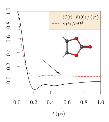
Figure 1: Velocity autocorrelation function and friction kernel $\gamma\left(t\right)$ defined with Eq. (1), for the center-of-mass of ethylene carbonate in neat liquid ethylene carbonate. See also Ref. 4. The arrow indicates the second-relaxation feature that is the primary phenomenon for these studies.

II Methods

We perform simulations (Table 1) of dilute and 1M solutions of LiPF₆ using the GROMACS molecular dynamics package with periodic boundary conditions. A Nose-Hoover thermostat^{9; 10} and a Parrinello-Rahman¹¹ barostat were utilized to achieve equilibration in the $NpT$ ensemble at 300 K and 1 atm pressure. A 10 ns simulation was carried out for aging, then a separate 1 ns simulation with a sampling rate of 1 fs was carried out to calculate the velocity autocorrelation and the friction kernel.

	Ions	Water	ACN	EC	PC
1M	32 Li+ $+$ 32 PF${}_{6}{}^{-}$	1776	613	480	378
dilute	1 Li+ / 1 PF${}_{6}{}^{-}$	999	449	249	249

Table 1: System sizes in dilute and concentrated solutions of 1M LiPF₆ in several solvents

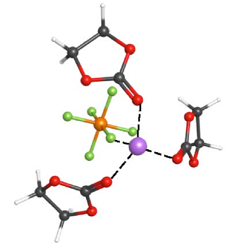
Figure 2: Optimized (EC)₃Li⁺…PF${}_{6}{}^{-}$ cluster, characterizing ion-paired structures of LiPF₆ in ethylene carbonate solvent. Gaussian09¹² was used for these electronic structure calculations at the Hartee-Fock level with 6-311+G(2d,p) basis set. Initial structures were sampled from MD simulations.

II.1 Forcefield parameters and adjustments

The interactions were modeled following the OPLS-AA forcefield¹³ with parameters as indicated below for bonded and non-bonded interactions. Li⁺ parameters were obtained from Soetens, et al.¹⁶ Partial charges of EC and PC were scaled ¹⁴ to match transport properties of Li⁺ with experiment. In the case of acetonitrile and water, standard OPLS-AA and SPC/E parameters were used.¹⁵

The PF${}_{6}{}^{-}$ ions were described initially with parameters from Sharma, et al.¹⁷ In initial MD trials, however, we observed PF${}_{6}{}^{-}$ ions that deviated significantly from octahedral geometries, particularly in the case of 1M LiPF₆ in EC, where substantial ion-pairing was observed. These PF${}_{6}{}^{-}$ displayed extreme bending of the axial F-P-F bond angles.

The possibility of exotic non-octahedral PF${}_{6}{}^{-}$ configurations in ion-paired (EC)₃Li⁺…PF${}_{6}{}^{-}$ clusters was investigated with electronic structure calculations. Gaussian09 calculations¹² employed the Hartee-Fock approximation with the 6-311+G(2d,p) basis set. Initial configurations were sampled from MD observations. The stable and lowest-energy clusters obtained were consistent with octahedral PF${}_{6}{}^{-}$ geometries (FIG. 2). We therefore increased the axial F-P-F (180$\degree$) bond-angle parameter by a factor of four in further MD calculations. The modified forcefield parameters for PF${}_{6}{}^{-}$ are provided with supplementary information.

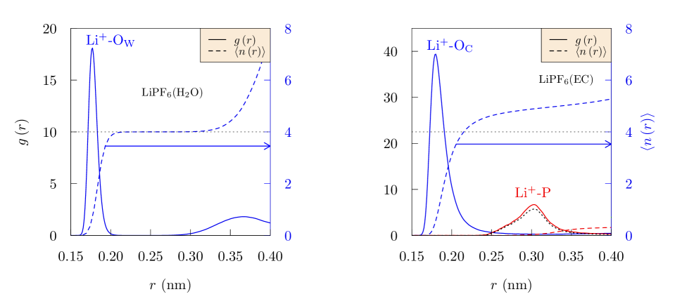
Figure 3: Radial distribution functions (solid curves, left axes), and the corresponding running coordination numbers (dashed, right axes). The right-pointing arrows indicate the axes for the coordination numbers $\langle{n(r)}\rangle$. Left panel: 1M LiPF₆ in water with $N_{\mathrm{W}}$ = 1776 water molecules. The extended $\langle{n(r)}\rangle=4$ plateau shows a distinct inner shell with that occupancy. Right panel: 1M LiPF₆ in ethylene carbonate with $N_{\mathrm{EC}}$ = 480 EC molecules. In contrast to the water case, a P atom is localized with the O_C inner shell. The black-dotted curve is $g\left(r\right)\exp\left\{-\langle{n(r)}\rangle\right\}$, the Fuoss/Poisson approximation¹⁸ to the distribution of the nearest P atom to a Li⁺ ion, supporting Li${}^{+}\cdots$ PF${}_{6}{}^{-}$ ion pairing at this concentration.

II.2 Solution structure

For Li⁺ in water, the oxygen coordination number is 4,^{19; 20; 21} with the inner-shell O atoms positioned at 0.18 nm. Similar Li⁺ coordination is observed in 1M solutions of LiPF₆ in PC and ACN.

In the case of 1M solutions in EC, the nearest Li-P peak centered at 0.33 nm (FIG. 3) indicates distinct but modest ion-pairing with PF${}_{6}{}^{-}$ at this concentration. The Fuoss/Poisson approximation¹⁸ is accurate here and that further supports the ion-pairing picture. Reflecting F atom penetration of the natural EC inner shell (FIG. 2), the Li⁺-O atom inner shell distribution is broader in EC than in water.

We re-emphasize that previous work¹⁴ scaled partial charges of the solvent EC molecules to match ab initio and experimental results for Li⁺ solvation and dynamics. Nevertheless, van der Waals interactions are a primary concern for description of realistic ion-pairing.

II.3 The friction kernel

We define the friction kernel $\gamma\left(t\right)$ (or memory function) by

$$m\frac{\mathrm{d}C(t)}{\mathrm{d}t}=-\int_{0}^{t}\gamma\left(t-\tau\right)C\left(\tau\right)\mathrm{d}\tau~{},$$ (1)

where $m$ is the mass of the molecule, and $C(t)$ is the velocity autocorrelation (VACF),

$$C(t)=\left\langle\vec{v}\left(t\right)\cdot\vec{v}\left(0\right)\right\rangle/\left\langle v^{2}\right\rangle~{}.$$ (2)

The friction kernel $\gamma\left(t\right)$ is the autocorrelation function of the random forces on a molecule.¹ The standard formality for extracting $\gamma\left(t\right)$ utilizes Laplace transforms. But inverting the Laplace transform is non-trivial and we have found the well-known Stehfest algorithm ²² to be problematic. Berne and Harp ²³ developed a finite-difference-in-time procedure for extracting $\gamma\left(t\right)$ from Eq. (1). That procedure is satisfactory, but sensitive to time resolution in the discrete numerical $C\left(t\right)$ used as input. An alternative⁴ expresses the Laplace transform as Fourier integrals, utilizing specifically the transforms

$$\hat{C}^{\prime}\left(\omega\right) =\int_{0}^{\infty}C(t)\cos\left(\omega t\right)\mathrm{d}t~{},$$ (3a)

$$\hat{C}^{\prime\prime}\left(\omega\right) =\int_{0}^{\infty}C(t)\sin\left(\omega t\right)\mathrm{d}t~{}.$$ (3b)

Then

$$\int_{0}^{\infty}\gamma(t)\cos\left(\omega t\right)\mathrm{d}t=\frac{m\hat{C}^{\prime}\left(\omega\right)}{\hat{C}^{\prime}\left(\omega\right)^{2}+\hat{C}^{\prime\prime}\left(\omega\right)^{2}}~{}.$$ (4)

Taking $\gamma\left(t\right)$ to be even time, the cosine transform is straightforwardly inverted. $\Omega^{2}=\left\langle F^{2}\right\rangle/3mk_{\mathrm{B}}T,$ with $F=|\vec{F}|$ the force on the molecule, provides the normalization $\gamma(0)=m\Omega^{2}.$ A comparison of these methods are provided in the supplementary information and Ref. 4.

III Results

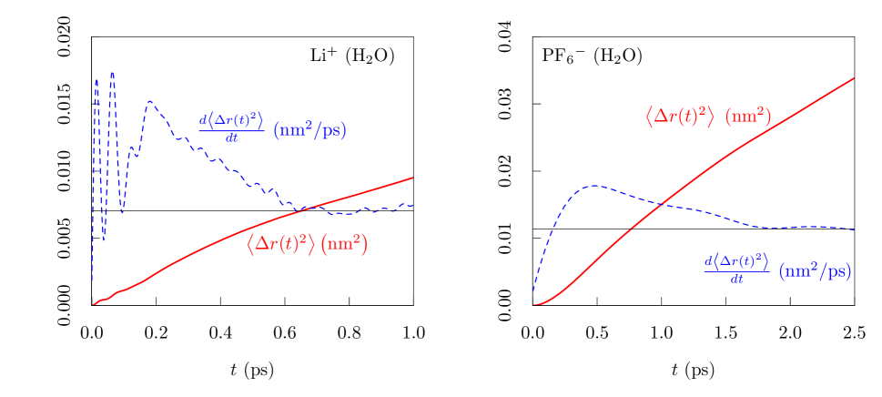
Figure 4: Comparison for Li⁺(aq) (left) and PF${}_{6}{}^{-}$(aq) (right) of the mean-squared-displacement (red) and its derivative (blue) with time. Oscillatory behavior for Li⁺ is prominent, not troublesome, and not evident in the corresponding results for PF${}_{6}{}^{-}$.

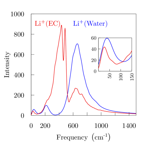
Figure 5: Power spectra (Eq. (3a)) of Li⁺ using the Gromacs velacc²⁴ utility. Red: 1M LiPF₆ in EC. To identify the predominant modes, electronic structure calculations using Gaussian09¹² software were performed with the b3lyp exchange-correlation density functional and 6-31+g(d,p) basis set. The frequency mode near 400 cm^-1 corresponds to motion of a Li⁺ ion trapped in a cage formed by its neighbors. The higher frequency band (near 650 cm^-1) corresponds to Li⁺ ion picking up the scissoring motion of a neighboring carbonate group. Blue: 1M LiPF₆ in Water. Here, the frequency band (near 650 cm^-1) corresponds to motion of a Li⁺ ion trapped in a cage formed by neighboring water molecules.

We discuss quantitative simulation results that lay a basis for molecule-specific theory of the friction coefficients of ions in solution. Our initial discussion focuses on dynamics of ions such as Li⁺ and PF${}_{6}{}^{-}$ in water, followed by overall comparisons with common non-aqueous solvents.

III.1 Oscillatory behavior of Li⁺ dynamics

The Li⁺ ion has an unusually small mass, and oscillatory behavior of its dynamics at short times is prominent compared to PF${}_{6}{}^{-}$. These differences are reflected in the mean squared displacement (FIG. 4) of these ions in water. This short-time behavior has been the particular target of the molecular time-scale generalized Langevin theory.²⁵ The vibrational power spectrum (FIG. 5) then provides a more immediate discrimination of the forces on the ions by the different solvents. Electronic structure calculations identify the high frequency vibrations that are related to motion of a Li⁺ trapped within an inner solvation shell. In the case of Li⁺(aq), this frequency occurs at 650 cm^-1. Nevertheless, the low frequency ($\omega\approx 0$) diffusive behavior can be only subtly distinct for different solution cases (FIG. 5), including electrolyte concentration (FIG. 6).

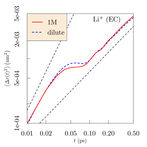
Figure 6: The mean-squared-displacement for Li⁺ ion in EC. The black dashed lines indicate slopes of initial ballistic and final diffusive behaviors. The asymptotic slope at long times is not significantly affected by concentration and the ion-pairing that is exhibited by this system.

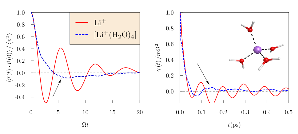
Figure 7: Left: Comparison of Li⁺ in water (red solid line) with center-of-mass of Li${}^{+}\left(\mathrm{H}_{2}\mathrm{O}\right)_{4}$ solventberg (blue dashed line indicated by the arrows). The horizontal axis is made dimensionless with the Einstein frequency $\Omega\equiv\sqrt{-C^{\prime\prime}\left(t=0\right)}$ evaluated numerically. These values are $\Omega\approx$ 590 cm^-1 and 116 cm^-1 for Li⁺(aq) and the Li⁺(H₂O)₄ solventberg, respectively. This means that the total temporal extent of the displayed relaxations are about five times longer for the Li⁺(H₂O)₄ solventberg results than for the Li⁺(aq). This time scaling results in matching the initial curvatures of the distinct functions shown here. The oscillations that are internal to the solventberg (inset on right) are not reflected in that VACF. The negative tail relaxation of the solventberg is then qualitatively similar to that of PF${}_{6}{}^{-}$ (see Fig. 8). Right: $\gamma\left(t\right)$ of the solventberg is also similar to PF${}_{6}{}^{-}$(aq) (Fig. 8).

III.2 Solventberg picture

A common view why the transport parameters can depend only weakly on the differences in the molecular-time-scale dynamics (FIG. 4) follows from the appreciation that the exchange time for inner shell solvent molecules can be long compared to the dynamical differences. For Li⁺(aq), that exchange time is of the order of 30 ps.^{26; 27} Then ion plus inner-shell solvent molecules — a solventberg³ — can be viewed as the transporting species.

The mean-squared displacement of the ion followed over times that are long on molecular time-scale but shorter than that exchange time should not differ much from the mean-squared displacement of the solventberg. The oscillations internal to the solventberg, which are reflected in the VACF, are not essential to the transport. Nevertheless, molecular dynamics simulation permits us to check the VACF of the center-of-mass of the solventberg. This VACF is free of oscillations and reveals a negative tail relaxation that is qualitatively similar to PF${}_{6}{}^{-}$ (FIG. 7). Indeed, previous calculations, treating both water^{28; 29} and EC,³⁰ fixed a Li⁺ ion coordinate for calculation of the force autocorrelation. Those prior works indeed also observed this second, longer time-scale relaxation that the present calculations highlight.

III.3 Overall comparisons

The overall comparisons of these single-ion VACFs and $\gamma\left(t\right)$ for our collection of solvents (FIG. 8) show these relaxations are similar to each other for the heavier ion PF${}_{6}{}^{-}$: a clear second relaxation for $\gamma\left(t\right)$ consistent with negative tail relaxations for the VACF. This behavior is similar for other molecular ions considered recently, and including $n$-pentanol as solvent.² Numerical VACF results for PF${}_{6}{}^{-}$(aq) show that the molecular time-scale relaxation is insensitive to electrolyte concentration and to van der Waals attractive forces (SI). For Li⁺, short time-scale oscillatory behavior masks that longer time-scale relaxation of $\gamma\left(t\right)$, as discussed above. Detailed results corresponding to FIG. 8 but for a Li⁺ ion are provided in the SI.

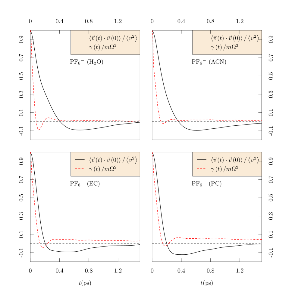
Figure 8: The center-of-mass VACF (black solid lines) and the corresponding friction kernel (red dashed lines), ${\scriptsize\gamma\left(t\right)}$, for PF${}_{6}{}^{-}$ from simulations of 1M LiPF₆ in several solvents. While ${\scriptsize\gamma\left(t\right)}$ is qualitatively similar at short and moderate times, the longer time-scale relaxation is more prominent for EC and PC compared to water and ACN. All 1M calculations consisted of 32 Li⁺ and PF${}_{6}{}^{-}$ ions together with the solvent molecule numbers that fix the specified molarity of the solution.

IV Conclusions

We extract the VACF and the memory function, $\gamma(t)$, which characterize the mobility of ions in solution. For the heavier PF${}_{6}{}^{-}$ ion, velocity relaxations are all similar: negative tail relaxations for the VACF and a clear second relaxation for $\gamma\left(t\right)$. For the light Li⁺ ion, analysis of the solventberg dynamics conform to the standard picture set by all the PF${}_{6}{}^{-}$ results. These results lay a quantitative basis for establishing a molecule-specific theory of the friction coefficients of ions in solution.

V SUPPLEMENTARY MATERIAL

The supplementary material provides a comparison of methods for extracting the friction kernel, a comparison of Li⁺ dynamics in different solvents, forcefield parameters for PF${}_{6}{}^{-}$ and the effect of removing van der Waals attractions on the dynamics of PF${}_{6}{}^{-}$(aq).

References

- Forster (1975) D. Forster, Hydrodynamic fluctuations, broken symmetry, and correlation functions, Frontiers in Physics, Vol. 47 (WA Benjamin, Inc., Reading, Mass., 1975).
- Zhu, Pratt, and Papadopoulos (2012) P. Zhu, L. Pratt, and K. Papadopoulos, J. Chem. Phys. 137, 174501 (2012).
- Wolynes (1978) P. G. Wolynes, J. Chem. Phys. 68, 473 (1978).
- You, Pratt, and Rick (2014) X. You, L. R. Pratt, and S. W. Rick, arXiv preprint arXiv:1411.1773 (2014).
- Zwanzig and Bixon (1970) R. Zwanzig and M. Bixon, Phys. Rev. A 2, 2005 (1970).
- Metiu, Oxtoby, and Freed (1977) H. Metiu, D. W. Oxtoby, and K. F. Freed, Phys. Rev. A 15, 361 (1977).
- Gaskell and Miller (1978) T. Gaskell and S. Miller, J. Phys. C: Solid State Physics 11, 3749 (1978).
- Balucani, Brodholt, and Vallauri (1999) U. Balucani, J. P. Brodholt, and R. Vallauri, J. Phys.: Condensed Matter 8, 6139 (1999).
- Nosé (1984) S. Nosé, Mol. Phys. 52, 255 (1984).
- Hoover (1985) W. G. Hoover, Phys. Rev. A 31, 1695 (1985).
- Parrinello and Rahman (1981) M. Parrinello and A. Rahman, J. App. Phys. 52, 7182 (1981).
- (12) M. J. Frisch, G. W. Trucks, H. B. Schlegel, and et. al., “Gaussian 09 Revision A.1,” Gaussian Inc. Wallingford CT 2009.
- Jorgensen and Maxwell (1996) W. L. Jorgensen and D. S. Maxwell, J. Am. Chem. Soc. 118, 11225 (1996).
- Chaudhari et al. (2016) M. I. Chaudhari, J. R. Nair, L. R. Pratt, F. A. Soto, P. B. Balbuena, and S. B. Rempe, J. Chem. Theory & Comp. 12, 5709 (2016).
- Berendsen, Grigera, and Straatsma (1987) H. Berendsen, J. Grigera, and T. Straatsma, J. Phys. Chem. 91, 6269 (1987).
- Soetens, Millot, and Maigret (1998) J.-C. Soetens, C. Millot, and B. Maigret, J. Phys. Chem. A 102, 1055 (1998).
- Sharma and Ghorai (2016) A. Sharma and P. K. Ghorai, J. Chem. Phys. 144, 114505 (2016).
- Zhu et al. (2011) P. Zhu, X. You, L. Pratt, and K. Papadopoulos, J. Chem. Phys. 134, 054502 (2011).
- Rempe et al. (2000) S. B. Rempe, L. R. Pratt, G. Hummer, J. D. Kress, R. L. Martin, and A. Redondo, J. Am. Chem. Soc. 122, 966 (2000).
- Alam, Hart, and Rempe (2011) T. M. Alam, D. Hart, and S. L. Rempe, Physical Chemistry Chemical Physics 13, 13629 (2011).
- Mason et al. (2015) P. Mason, S. Ansell, G. Neilson, and S. Rempe, J. Phys. Chem. B 119, 2003 (2015).
- Stehfest (1970) H. Stehfest, Comm. ACM 13, 47 (1970).
- Berne and Harp (1970) B. J. Berne and G. D. Harp, Adv. Chem. Phys 17, 63 (1970).
- Abraham et al. (2014) M. Abraham, D. Van Der Spoel, E. Lindahl, and B. Hess, “The GROMACS development team GROMACS user manual version 5.0.4,” (2014).
- Adelman (1980) S. Adelman, Adv. Chem. Phys. 44, 143 (1980).
- Friedman (1985) H. Friedman, Chemica Scripta 25, 42 (1985).
- Dang and Annapureddy (2013) L. X. Dang and H. V. R. Annapureddy, J. Chem. Phys. 139, 084506 (2013).
- Annapureddy and Dang (2012) H. V. R. Annapureddy and L. X. Dang, J. Phys. Chem. B 116, 7492 (2012).
- Annapureddy and Dang (2014) H. V. R. Annapureddy and L. X. Dang, J. Phys. Chem. B 118, 8917 (2014).
- Chang and Dang (2017) T.-M. Chang and L. X. Dang, J. Chem. Phys. 147, 161709 (2017).
- Weeks, Chandler, and Andersen (1971) J. D. Weeks, D. Chandler, and H. C. Andersen, J. Chem. Phys. 54, 5237 (1971).