Orbital stability in static axisymmetric fields
Abstract
We investigate the stability of test-particle equilibrium orbits in axisymmetric, but otherwise arbitrary, gravitational and electromagnetic fields. We extend previous studies of this problem to include a toroidal magnetic field. We find that, even though the toroidal magnetic field does not alter the location of the circular orbits, it enters the problem as a gyroscopic force with the potential to provide gyroscopic stability. This is in essence similar to the situation encountered in the reduced three-body problem where rotation enables stability around the local maxima of the effective potential. Nevertheless, we show that gyroscopic stabilization by a toroidal magnetic field is impossible for axisymmetric force fields in source-free regions because in this case the effective potential does not possess any local maxima. As an example of an axisymmetric force field with sources, we consider the classical problem of a rotating, aligned magnetosphere. By analyzing the dynamics of halo and equatorial particle orbits we conclude that axisymmetric toroidal fields that are antisymmetric about the equator are unable to provide gyroscopic stabilization. On the other hand, a toroidal magnetic field that does not vanish at the equator can provide gyroscopic stabilization for positively charged particles in prograde equatorial orbits.
1 Introduction
The study of particle dynamics in axisymmetric fields is important in a variety of problems spanning a wide range of scales in nature. The axial symmetry can be exploited to reduce the number of degrees of freedom. In the reduced phase space, the scalar potential, which conservative forces derive from, is replaced by an effective potential that includes the toroidal kinetic energy. Critical points of the effective potential are equilibria of the reduced system. These correspond to circular orbits in three-dimensional space. Howard (1999) provides a thorough overview of the stability of circular orbits in axisymmetric gravitational and electromagnetic fields. The magnetic fields considered there are assumed to be purely poloidal. While this is a reasonable assumption to make in many axisymmetric systems, it is not difficult to think of examples where toroidal magnetic fields play a significant role. Such examples include toroidal fusion devices and galactic disks.
In this paper, we generalize Howard (1999) analysis addressing the stability of circular orbits by including a toroidal axisymmetric magnetic field. Axisymmetric poloidal and toroidal magnetic fields enter the dynamics in a fundamentally different way. All the effects related to the poloidal magnetic field can be encapsulated in the effective potential together with the gravitational contribution, whereas this is never the case for the toroidal part. As we detail below, this crucial difference makes it possible for the toroidal magnetic field to provide stability in regions of parameter space where a purely poloidal field cannot. This is a manifestation of the phenomenon known as gyroscopic stability, which is usually associated with the Coriolis force.
The rest of the paper is organized as follows. In section 2 we state the equations of motion for a test particle in reduced phase space by introducing the Routhian and an effective potential that depends only on the poloidal flux function. In section 3 we analize the stability of circular orbits and find the conditions for gyroscopic stabilization via a toroidal magnetic field. In particular, we show that in source-free regions, gyroscopic stabilization via a toroidal magnetic field is impossible. In section 4 we illustrate some of the implications of our findings by analysing the problem of a rotating magnetosphere. We conclude by discussing our results in section 5.
2 Equations of motion
The motion of a classical, non-relativistic111This is the most general single particle Lagrangian compatible with Galilean invariance (Jauch, 1964; Roman and Leveille, 1974). particle is governed by the Lagrangian per unit particle mass
| (1) |
where denotes the time derivative of the particle’s position vector. We have absorbed the coupling constants (i.e., charge and mass) in the scalar potential and the vector potential , both of which are assumed time-independent. In the following, we will refer to and as electromagnetic potentials. Note, however, that can include the gravitational potential and/or the centrifugal potential and can include a contribution accounting for the Coriolis force that arises in a rotating frame. The equation of motion derived from eq. 1 via the Euler-Lagrange equation is , where the electric field is and the magnetic field is . We note that if only electromagnetic forces are present, then and differ from the true electromagnetic fields by a factor equal to the charge-to-mass ratio.
2.1 Motion in reduced phase space
We work in cylindrical coordinates and assume that the system is symmetric about the -axis. This means that neither nor depend on the cyclic coordinate . From the Euler-Lagrange equation it then follows that the generalized angular momentum is an integral of motion. Substituting eq. 1 we obtain
| (2) |
where we have introduced the poloidal flux function
| (3) |
in terms of which the magnetic field is given by .
Since is an integral of motion, the dimensionality of the problem may be reduced by one. For this we introduce the Routhian , where
| (4) |
is equal to the angular velocity expressed through eq. 2 as a function of and . With eq. 4 the Routhian is given by
| (5) |
where
| (6) |
is the effective potential.
The equations of motion of the reduced system are for or
| (7) | ||||
These equations possess the energy integral
| (8) |
which evidently is independent of the toroidal magnetic field. This is because the force due to the toroidal magnetic field does not do work in the reduced configuration space. Such forces are called gyroscopic forces (Thomson and Tait, 1883a, b). Very much in contrast to this, the force due to the poloidal magnetic field, which in fact is gyroscopic before reduction, has become a potential force in the reduced configuration space. A reduced system of the form 7 with is said to be gyroscopically constrained or coupled (see e.g. Rumiantsev, 1966; Merkin, 1996).
2.2 Hamiltonian formalism
Before moving on to study the stability of equilibrium solutions of the equations of motion, we note that the reduced system may also be described using a Hamiltonian formalism. In a gyroscopically coupled system this is best done by working in non-canonical phase space coordinates
| (9) |
see e.g. Littlejohn (1979, 1982) or Bolotin and Negrini (1995). In these coordinates, the equations of motion are
| (10) |
where the Hamiltonian is defined in eq. 8 and the Poisson matrix is given by
| (11) |
It is straightforward to verify that given the definitions in eqs. 10 and 11, Hamilton’s equations in the form of eq. 10 are equivalent to the equations of motion 7. We also note that the Poisson bracket defined by satisfies the Jacobi identity for any , as it should.
3 Stability of circular orbits
In this section we discuss the stability of equilibrium solutions to the equations of motion 7. We note that all that is said here in fact holds for arbitrary forms of the effective potential. This means that for instance the restricted three-body problem is within the scope of our discussion. Only in section 4 will we specialize to effective potentials of the form given in eq. 6, in which the scalar potential is independent of the canonical angular momentum .
3.1 Stability criteria
Equilibria of the reduced system described by eq. 5 are solutions with . The angular velocity is, however, in general non-zero. Equilibria of the reduced system thus correspond to uniformly rotating solutions of the original system. In the classic literature (e.g. Routh, 1884), such solutions are known as steady motions. A more modern term is relative equilibria (e.g. Marsden and Weinstein, 1974).222It should be noted that relative equilibria potentially encompass a much wider class of solutions than just steady motions. Like steady motions, relative equilibria are obtained by reduction through symmetry, but unlike steady motions, relative equilibria allow for the underlying symmetry group to be non-Abelian. In the following we will refer to these solutions simply as circular orbits.
Inspection of the equations of motion 7 reveals that circular orbits are stationary points of the effective potential, i.e. points at which for arbitrary variations and . Their location is evidently independent of the toroidal magnetic field . This agrees with the expectation that because the magnetic force is perpendicular to the velocity, the toroidal magnetic field should of course have no effect on strictly circular orbits.
Whether or not circular orbits can be expected to actually occur in nature (along with nearly circular orbits in their vicinity) depends on their stability. Various notions of stability exist in the literature (see e.g. Holm et al., 1985). Arguably the most important one for practical purposes is due to Lyapunov: an equilibrium , with defined in eq. 9, is stable for every if there is a such that if then for . It is important to note that in this definition evolves according to the nonlinear equations of motion 10. By contrast, spectral stability is concerned with the spectrum of the Hamiltonian matrix , obtained by linearizing eq. 10. A Hamiltonian system is spectrally stable if all eigenvalues of this matrix lie on the imaginary axis. Lyapunov stability implies spectral stability but not vice versa (Holm et al., 1985). In the following, stability will generally be synonymous with Lyapunov stability — the stronger of the two notions — unless specified otherwise.
The discussion in the above paragraph has an important caveat: the canonical angular momentum (the cyclic integral) is assumed fixed. Truly arbitrary perturbations would also allow to be varied. It is often argued that in practice the restriction of fixed cyclic integrals is unimportant because, as Pars (1965) writes, “if we do allow small changes in the [cyclic integrals] we are merely transferring our attention to oscillations about a neighboring state of steady motion.” This argument is originally due to Lyapunov (see Rumiantsev, 1966). It may of course be that there is no neighboring state of steady motion, in which case this argument fails and a more elaborate approach becomes necessary (Salvadori, 1953). A comprehensive discussion is given by Hagedorn (1971). In the following we will ignore these subtleties and take as fixed.
According to Routh’s theorem (Routh, 1884), a circular orbit is stable if it corresponds to an isolated minimum of the effective potential. This is the case if the second variation for any non-zero and/or . Expressed in terms of the Hessian of the effective potential, whose trace and determinant are given by
| (12) |
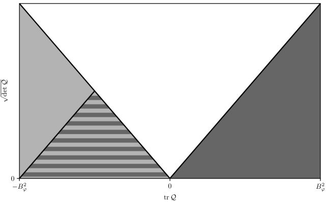
a critical point of the effective potential is an isolated minimum if and only if
| (13) |
If the inequalities in eq. 13 are satisfied, then the total energy at equilibrium is positive definite (i.e. for any non-zero ) and can thus be used as a Lyapunov function to prove Routh’s theorem using Lyapunov’s direct method (Merkin, 1996). In the absence of a toroidal magnetic field (), in which case the system is gyroscopically decoupled, the converse is also true (Lyapunov, 1907; Malkin, 1959; Chetaev, 1961; Hagedorn, 1971; Rumyantsev and Sosnitskii, 1993): circular orbits are unstable if they do not minimize locally.
3.2 Gyroscopic stabilization
In the presence of a toroidal magnetic field, the system is gyroscopically coupled. In this case, all circular orbits located at isolated minima of are still stable. However, there may now also exist stable circular orbits located at isolated maxima of the effective potential, where . This is known as gyroscopic stabilization (Thomson and Tait, 1883a, b; Chetaev, 1961; Merkin, 1996). All orbits are spectrally unstable at saddle points ().
A note about energetics is in order here. Isolated minima of the effective potential correspond to isolated minima of the total energy because the kinetic energy is positive definite. In other words . Definiteness of is referred to as formal or energetic stability (Holm et al., 1985; Scheeres, 2006). It is a sufficient but not necessary condition for Lyapunov stability. The toroidal magnetic field does not affect the energetic stability of circular orbits. It can, however, stabilize energetically unstable orbits, namely isolated maxima of , for which is indefinite because .
In order to determine the conditions for gyroscopic stabilization to occur, we first carry out a spectral stability analysis. Considering infinitesimal perturbations of the linearized equations of motion eq. 7 leads to the characteristic polynomial
| (14) |
The roots of this equation comprise the spectrum of the Hamiltonian matrix mentioned above. A comprehensive discussion of eq. 14 is given in Bloch et al. (1994), see also Chetaev (1961) and Haller (1992). Isolated maxima of the effective potential are critical points where or, equivalently, and . Depending on the strength of the toroidal field, only a subset of these maxima are gyroscopically stabilized. The precise conditions are
| (15) |
Note that for a given maximum of the effective potential, it is always possible to satisfy these inequalities for large enough . A visual representation of the inequalities in eqs. 13 and 15 is given in fig. 1.
If the inequalities in eq. 15 are satisfied, then the circular orbit is gyroscopically stabilized in the spectral sense: all eigenvalues as given by the roots of eq. 14 lie on the imaginary axis. In order to show that circular orbits can be gyroscopically stabilized in the Lyapunov sense is more challenging. Since is negative definite at an isolated maximum, the total energy defined in eq. 8 is indefinite and thus cannot be used as a Lyapunov function to prove stability using the direct method.
Instead, Lyapunov stability at isolated maxima of the effective potential can be demonstrated with the help of the Kolmogorov-Arnold-Moser (KAM) theorem. At a spectrally stable isolated maximum, where eqs. 15 are satisfied, the eigenvalues and of the linearized system, given by the roots of the characteristic polynomial 14, are purely imaginary. If these eigenvalues are non-resonant ( for ), then the nonlinear dynamics of the system close to equilibrium is nearly integrable. The integrable, linear dynamics takes place on two-dimensional tori in phase space and the KAM theorem ensures these tori persist under nonlinear perturbations, provided certain non-degeneracy conditions are met (Arnold, 1963; Haller, 1992). Note that since is assumed fixed, these considerations strictly speaking only demonstrate conditional Lyapunov stability for the reduced system.
It is important to stress that both resonance and degeneracy occur with probability zero in continuous (real valued) parameter space. Moreover, if the system is resonant it may still be stable (Sokolskii, 1974). Likewise, non-degeneracy is sufficient but not necessary for stability: in systems with two degrees of freedom (such as the present one) degenerate equilibria are, as a rule, stable (Arnold et al., 2006, sec. 6.3.6.B).
3.3 The effects of dissipation
The above considerations need to be amended if the system is dissipative. Minima of the effective potential remain stable when dissipation is added to the system, however, all other equilibria are unstable no matter how small (but finite) the dissipation is. In particular, gyroscopically stabilized equilibria, which correspond to maxima of the effective potential, lose their stability if dissipation is added (Thomson and Tait, 1883a, b; Chetaev, 1961; Rumiantsev, 1966; Haller, 1992). Loss of gyroscopic stabilization due to dissipation is an instance of a wider class of phenomena known as dissipation-induced instabilities (Bloch et al., 1994; Krechetnikov and Marsden, 2007).
In practice gyrcosopic stabilization is thus only a transient phenomenon. The growth rate of these instabilities, which are generally proportional to the dissipation rate (MacKay, 1991; Bloch et al., 1994), is much smaller than the growth rates in the absence of gyroscopic forces. Thomson and Tait (1883a, b) refer to this as temporary, as opposed to secular, stability.
The fact that in realistic systems, gyroscopic forces are not able to truly stabilize an otherwise unstable equilibrium does not diminish the significance of gyroscopic stabilization by very much. This can be seen in the restricted three-body problem applied to the Sun-Jupiter system. The critical points of the effective potential in this problem are either saddle points (, , and ) or local maxima ( and ). Gyroscopic stability at and is provided by the Coriolis force. The Trojan asteroids are are found to cluster around and even though they are subject to a dissipative force due to nebular drag and hence to dissipation induced instability.
3.4 Impossibility of gyroscopic stabilization in source-free regions
In the previous section we have seen that whether gyroscopic stabilization is possible depends on the sign of . In order to calculate the trace Hessian, we need to compute its diagonal elements. These are given by
| (16) |
where the poloidal magnetic field components are and . Adding up eq. 16 yields the trace of the Hessian. The resulting expression can be simplified with the help of Gauss’ law , i.e.
| (17) |
and Ampère’s law , whose toroidal component is given by
| (18) |
In the plasma physics literature, the differential operator acting on in eq. 18 is known as the Grad-Shafranov operator (see e.g. Almaguer et al., 1988). With eqs. 17 and 18, evaluating the trace at equilibrium yields
| (19) |
where we have used
| (20) |
The first three terms on the right hand side of eq. 19 are all non-negative. Thus, in source-free regions, where and , the effective potential has no local maxima and gyroscopic stabilisation cannot occur. We note that matter distributions make a negative contribution to and hence a positive contribution to . We also note that poloidal currents, i.e. sources of the toroidal magnetic field, do not enter eq. 19 at all.
In addition to physical sources in the form or matter and charge distributions there may also be fictitious sources that arise in a rotating frame. For instance, associated with the centrifugal force is a fictitious charge distribution . That being said, in appendix A we show that the stability of circular orbits is not affected by a transformation to a rotating frame of reference.
4 Motion in a rotating magnetosphere
As an example of astrophysical relevance where gyroscopic stability by a toroidal magnetic field is possible we analyse the stability of circular orbits in the classical problem of a rotating magnetosphere. We consider the same model studied by Howard et al. (1999, 2000) and Dullin et al. (2002), where the poloidal magnetic field and the planetary gravitational potential are due to a point dipole and a point mass, respectively.
The poloidal flux function is given by
| (21) |
where is the spherical radius. The parameter is proportional to the product of the charge to mass ratio and the dipole strength. Without loss of generality we take the magnetic dipole to point along the -axis. With this convention, for positive charges. The poloidal magnetic field components and derived from eq. 21 are
| (22) |
The scalar potential is
| (23) |
The first term is the gravitational potential. The second term arises from the requirement that the electric field vanishes in a frame rotating with the planetary rotation rate .
The current density that derives from eq. 21 via Ampère’s law 18 vanishes away from the origin. However, the charge density that derives from eq. 23 via Gauss’ law 17 does not vanish and is given by
| (24) |
for . This charge density, known in the astrophysical literature as the Goldreich-Julian charge density (Goldreich and Julian, 1969), is distributed continuously throughout space. Because of this, positivity of the trace in eq. 19 is no longer ensured.
In order to assess what orbits can be subject to gyroscopic stabilisation, we analyse the characteristics of equilibria, focusing our attention on the regions of parameter space associated with negative . The calculations involved in obtaining and in eq. 12 have already been carried out in Dullin et al. (2002). For the reader’s convenience, and because we use different notation, we restate the results that are relevant to the discussion here.
Using eq. 21 and eq. 23 we obtain the location of the equilibrium circular orbits by requiring that the first variation of the effective potential in eq. 6 vanishes, i.e. by requiring
| (25) | ||||
| (26) |
Setting to zero each of the two factors on eq. 26 leads to equatorial and halo orbits respectively. We analyse each of these cases separately.
4.1 Equatorial orbits
Equatorial orbits lie within the plane . Their radial location is obtained from eq. 25 with . The result is
| (27) |
The determinant and trace of the Hessian evaluated at equatorial equilibria are given by
| (28) |
and
| (29) |
From these expressions we can easily compute the zeros of both and and characterise the various regions of parameter space according to their stability properties. The results are illustrated in fig. 2, which is almost identical to Figure 7 in Dullin et al. (2002), except that we also plot the curve along which the trace vanishes.
In addition to the two energetically stable regions identified already by Dullin et al. (2002), there is now a region spanned by orbits corresponding to particles with positive charge () in prograde rotation (). These orbits can be stabilized via gyroscopic effects provided a sufficiently strong toroidal field is present. We remark, however, that this is unlikely to be the case as the toroidal field is typically anti-symmetric about the equator in realistic magnetospheres (see e.g. Bunce and Cowley, 2001).

4.2 Halo orbits
The coordinates for circular halo orbits are obtained by setting to zero the second term in eq. 26 and using this result in eq. 25. This leads to
| (30) |
where is the angle subtended between the radius vector and the -direction such that and .
The determinant and trace of the Hessian evaluated at halo equilibria are given by
| (31) |
and
| (32) |
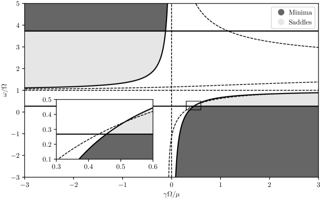
The regions of stability that derive from determining the signs of both and are illustrated in fig. 3. This figure is similar to Figure 9 in Dullin et al. (2002), except that we also plot the curve along which the trace vanishes. Close inspection of this figure, see in particular the inset, reveal that there are no regions where and . We thus conclude that gyroscopic stabilization of halo orbits via a toroidal magnetic field is impossible in an aligned dipolar magnetosphere.
5 Summary and Discussion
Howard (1999) presented an overview of the stability of circular orbits in combined axisymmetric gravitational and poloidal magnetic fields. In this case, orbital stability is completely determined by the effective potential, which contains all the dynamical effects arising from the magnetic field. Under these assumptions, because the kinetic energy is positive definite, equilibria are stable if and only if they minimize the effective potential.
In this paper, we have generalized this problem by including an axisymmetric toroidal magnetic field, which cannot be included in the effective potential. We pointed out that, unlike the poloidal field component, the toroidal magnetic field does no work in the reduced phase space, i.e., the magnetic force associated with it is gyroscopic333We point out that forces that are gyroscopic in three-dimensional space do not necessarily act as gyroscopic forces in the reduced space. This is indeed the case for a purely poloidal axisymmetric magnetic field. We also note the Lagrangian can acquire gyroscopic terms in the reduced space even in the absence of gyroscopic forces in three-dimensional space.. Thus even thought the toroidal field does not influence the location of the circular orbits it can alter their stability properties by enabling gyroscopic stability.
Absent dissipation, we carried out a spectral stability analysis and determined the conditions for gyroscopic stabilization by an axisymmetric toroidal magnetic field and summarized our results in fig. 1. We showed that, given a circular orbit in an isolated local maxima of the effective potential, it is always possible to find a sufficiently strong axisymmetric toroidal magnetic field to gyroscopically stabilise it. Making use of the KAM theorem we concluded that gyroscopic stability holds in the Lyapunov sense. In real systems, dissipative processes prevent gyroscopic stability from being truly realized. Nevertheless, this type of dissipation induced instabilities evolve on timescales that are much longer than the growth rates of instabilities that would operate in the absence of gyroscopic stabilization. We thus argue that gyroscopic stabilization should be relevant.
We showed that the effective potential associated with combined axisymmetric gravitational and poloidal magnetic fields does not present isolated local maxima in source free regions, thus implying that gyroscopic stabilisation is impossible in this case. As an example where sources are present, we considered a rotating, aligned magnetosphere and investigated the effects of a toroidal magnetic field. This is a generalization of the problem investigated by Howard, who provided a detailed account of the stability properties of equatorial (Howard et al., 1999) and halo (Howard et al., 2000) orbits of charged dust-particles for an aligned, rotating dipole. We found that there are no equilibrium halo orbits that can be subject to gyroscopic stabilisation. We also found, however, that there do exist prograde equatorial orbits for positive charges for which a toroidal magnetic field that does not vanish at the equator provides gyroscopic stabilization.
Appendix A Circular orbits in a rotating frame
Let us carry out a coordinate transformation to a frame rotating with a constant frequency around the -axis. The angular velocity in the rotating frame is
| (33) |
The transformed scalar potential and the poloidal flux function are respectively given by
| (34) |
and
| (35) |
The second term on the right hand side of eq. 34 arises because the electrostatic potential transforms as the temporal component of an ultra space-like four-vector (). The last terms in eqs. 34 and 35 account for the centrifugal force and the Coriolis force, respectively.
From eq. 35 it follows that the generalized angular momentum, defined in eq. 2, is invariant, i.e.
| (36) |
Given the transformations in eqs. 34, 35 and 36, the effective potential transforms according to
| (37) |
This is obviously consistent with eq. 33 since . From eq. 37 it follows immediately that
| (38) |
for arbitrary variations and . This means that neither the location of circular orbits nor their energetic stability is affected by a transformation to a rotating frame of reference.
In the rotating frame, the components of the poloidal electric field are given by
| (39) | ||||
The second term on each right hand side arise simply from a Galilean transformation with relative velocity . The last term in eq. 39 is the centrifugal force. The components of the transformed poloidal magnetic field are
| (40) | ||||
which include the Coriolis force. The toroidal component of the magnetic field is invariant. In light of eqs. 14 and 38 this means that the spectral stability of circular orbits is not affected either by a transformation to rotating frame of reference.
From Gauss’ law 17 and Ampère’s law 18 it follows that
| (41) |
and . It is easy to check that these transformations together with eqs. 33 and 40 indeed leave the trace of the Hessian as given in eq. 19 invariant.
Equation 41 shows that regions of space that are source-free in an inertial frame are not source-free in a rotating frame. We stress, however, that the last term in eq. 41 is not a physical source of either the electromagnetic or gravitational fields, but is a fictitious charge density that derives from the centrifugal potential via Gauss’ law 17.
Acknowledgements.
We thank Pablo Benítez-Llambay, Luis García-Naranjo and Jihad Touma for insightful comments. We are grateful for the hospitality of the Institute for Advanced Study where part of this work was carried out. The research leading to these results has received funding from the European Research Council (ERC) under the European Union’s Seventh Framework programme (FP/2007–2013) under ERC grant agreement No 306614.References
- Howard (1999) J. E. Howard, Celestial Mechanics and Dynamical Astronomy 74, 19 (1999).
- Jauch (1964) J. M. Jauch, Helvetica Physica Acta 37, 284 (1964).
- Roman and Leveille (1974) P. Roman and J. P. Leveille, Journal of Mathematical Physics 15, 1760 (1974).
- Thomson and Tait (1883a) W. Thomson and P. G. Tait, Treatise on Natural Philosophy (Vol 1) (Cambridge University Press, Cambridge, 1883).
- Thomson and Tait (1883b) W. Thomson and P. G. Tait, Treatise on Natural Philosophy (Vol 2) (Cambridge University Press, Cambridge, 1883).
- Rumiantsev (1966) V. Rumiantsev, Journal of Applied Mathematics and Mechanics 30, 1090 (1966).
- Merkin (1996) D. R. Merkin, Introduction to the Theory of Stability, Texts in Applied Mathematics, Vol. 24 (Springer New York, New York, NY, 1996).
- Littlejohn (1979) R. G. Littlejohn, Journal of Mathematical Physics 20, 2445 (1979).
- Littlejohn (1982) R. G. Littlejohn, Journal of Mathematical Physics 23, 742 (1982).
- Bolotin and Negrini (1995) S. Bolotin and P. Negrini, Nonlinear Differential Equations and Applications NoDEA Springer Monographs in Mathematics, 2, 417 (1995).
- Routh (1884) E. J. Routh, The Advanced Part of a Treatise on the Dynamics of a System of Rigid Bodies (Cambridge University Press, Cambridge, 1884).
- Marsden and Weinstein (1974) J. E. Marsden and A. Weinstein, Reports on Mathematical Physics 5, 121 (1974).
- Holm et al. (1985) D. D. Holm, J. E. Marsden, T. Ratiu, and A. Weinstein, Physics Reports 123, 1 (1985).
- Pars (1965) L. A. Pars, A Treatise on Analytical Dynamics (Heinemann, London, 1965).
- Salvadori (1953) L. Salvadori, Rend. Accad. Sci. fis. e math. Soc. nza. lett. ed arti. Napoli 20, 269 (1953).
- Hagedorn (1971) P. Hagedorn, Archive for Rational Mechanics and Analysis 42, 281 (1971).
- Lyapunov (1907) A. Lyapunov, Annales de la Faculté des sciences de Toulouse: Mathématiques 9, 203 (1907).
- Malkin (1959) J. G. Malkin, Theorie der Stabilität einer Bewegung (Akademie-Verlag, Berlin, 1959).
- Chetaev (1961) N. G. Chetaev, The Stability of Motion (Pergamon Press, Oxford, 1961).
- Rumyantsev and Sosnitskii (1993) V. V. Rumyantsev and S. P. Sosnitskii, Journal of Applied Mathematics and Mechanics 57, 1101 (1993).
- Scheeres (2006) D. J. Scheeres, Celestial Mechanics and Dynamical Astronomy 94, 317 (2006).
- Bloch et al. (1994) A. Bloch, P. S. Krishnaprasad, J. E. Marsden, and T. Ratiu, Annales de l’Institut Henri Poincaré (C) Analyse Non Linéaire 11, 37 (1994).
- Haller (1992) G. Haller, International Journal of Non-Linear Mechanics 27, 113 (1992).
- Arnold (1963) V. I. Arnold, Russian Mathematical Surveys 18, 85 (1963).
- Sokolskii (1974) A. G. Sokolskii, Journal of Applied Mathematics and Mechanics 38, 741 (1974).
- Arnold et al. (2006) V. I. Arnold, V. V. Kozlov, and A. I. Neishtadt, Mathematical Aspects of Classical and Celestial Mechanics, Encyclopaedia of Mathematical Sciences, Vol. 3 (Springer Berlin Heidelberg, Berlin, Heidelberg, 2006).
- Krechetnikov and Marsden (2007) R. Krechetnikov and J. E. Marsden, Reviews of Modern Physics 79, 519 (2007).
- MacKay (1991) R. S. MacKay, Physics Letters A 155, 266 (1991).
- Almaguer et al. (1988) J. A. Almaguer, E. Hameiri, J. Herrera, and D. D. Holm, Physics of Fluids 31, 1930 (1988).
- Howard et al. (1999) J. E. Howard, M. Horányi, and G. R. Stewart, Physical Review Letters 83, 3993 (1999).
- Howard et al. (2000) J. E. Howard, H. R. Dullin, and M. Horányi, Physical review letters 84, 3244 (2000).
- Dullin et al. (2002) H. R. Dullin, M. Horányi, and J. E. Howard, Physica D: Nonlinear Phenomena 171, 178 (2002).
- Goldreich and Julian (1969) P. Goldreich and W. H. Julian, The Astrophysical Journal 157, 869 (1969).
- Bunce and Cowley (2001) E. J. Bunce and S. W. H. Cowley, Planetary and Space Science 49, 1089 (2001).