Virtualization-based Evaluation
of Backhaul Performance in Vehicular Applications

Abstract

Next-generation networks, based on SDN and NFV, are expected to support a wide array of services, including vehicular safety applications. These services come with strict delay constraints, and our goal in this paper is to ascertain to which extent SDN/NFV-based networks are able to meet them. To this end, we build and emulate a vehicular collision detection system, using the popular Mininet and Docker tools, on a real-world topology with mobility information. Using different core network topologies and open-source SDN controllers, we measure (i) the delay with which vehicle beacons are processed and (ii) the associated overhead and energy consumption. We find that we can indeed meet the latency constraints associated with vehicular safety applications, and that SDN controllers represent a moderate contribution to the overall energy consumption but a significant source of additional delay.

1 Introduction

Vehicular networks are mobile wireless networks whose nodes are represented by connected vehicles and the infrastructure supporting them, e.g., road-side units (RSUs) providing Internet connectivity, as exemplified in Fig. 1. Current and expected applications abound, and include navigation, e.g., downloading maps or traffic updates, and entertainment, e.g., streaming movies to on-board entertainment systems similar to those found on airplanes.

A third, and arguably more critical, application of vehicular networks is represented by safety: indeed, in 2015 road accidents accounted for over 35,000 deaths in the United States alone [1], and over one million worldwide [2]. The most significant of these safety applications is collision detection. The idea of collision detection is fairly simple, and is summarized in Fig. 1. Vehicles periodically [3] (and anonymously [4]) report their position, direction and speed to a detector. The communication between vehicles and detectors happens through road-side units (RSUs), that make communication possible even in non-line-of-sight (NLoS) conditions, e.g., due to buildings or other obstacles. The detector combines these reports, determines whether any two vehicles are set on a collision course, and, if so, it alerts their drivers. Collision detection is especially important in presence of obstacles, e.g., buildings, that prevent drivers from timely realizing the danger. The importance and relevance of collision detection has been acknowledged by transportation regulators: as recently as December 2016, the U.S. Department of Transportation (DOT) published a Notice of Proposed Rulemaking (NPRM) for vehicular communications [5]. The document proposes to establish a new Federal Motor Vehicle Safety Standard (FMVSS), No. 150, to make vehicular networking technology compulsory: 50% of newly-made vehicles will have to be equipped with such a technology in 2018, 75% in 2019, and 100% in 2020.

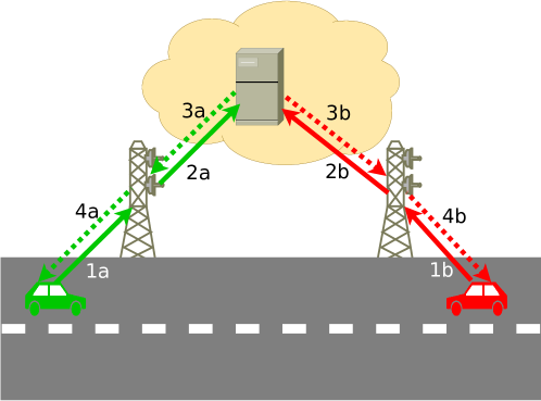
Figure 1: A simple vehicular network composed of two vehicles (red and green), two road-side units (RSUs) and a centralized collision detector. Solid lines represent beacon transmissions, dashed lines correspond to collision warnings. The vehicles periodically transmit beacons (1a, 1b), which, through the RSUs, reach the collision detector (2a, 2b). The detector realizes that the vehicles are set on a collision course, and issues two collision warnings (3a, 3b) that, again through the RSUs (4a, 4b), reach the vehicles.

It is fairly obvious that timeliness is critical to collision detection systems. However, satisfying latency requirements in emerging mobile network systems, which rely on software-defined networking (SDN) and network function virtualization (NFV) in the backhaul (and sometimes even in the fronthaul), may be challenging. Indeed, while SDN and NFV bring major improvements in terms of network flexibility and efficiency, both imply a certain amount of overhead: such overhead is negligible in most applications, but not when it comes to vehicular safety. An additional concern is represented by energy consumption: some network nodes, e.g., solar-powered RSUs, might not be connected to a reliable power supply; it is therefore important to know the power consumption associated with virtual network functions (VNFs), so as to better decide at which physical nodes to place them.

In this paper, we build, optimize, and evaluate a collision detection system, based on Mininet and Docker, the standard tools for SDN emulation and containerization, respectively. Our purpose is twofold: on the one hand, we study the impact of SDN and NFV on the performance of vehicular networks; on the other, we seek to learn valuable, real-world lessons concerning the pitfalls and implementation issues associated with our tools.

As far as the tools we use are concerned, Mininet [6] recently emerged as the de facto standard for reproducible network experiments. It emulates a full network, including software, SDN-capable switches and virtual hosts, running arbitrary programs in separate execution environments while sharing the file system and process space. It is typically used in SDN research, with custom-written controllers controlling the Mininet-emulated switches. In our case, however, we do not write our own custom controller; rather, we test two popular, general-purpose SDN controllers – namely, Pox [7] and Floodlight [8] – and ascertain how they impact the performance and energy consumption of our emulated network.

In our experiments, we couple Mininet with Docker [9], again the de facto standard containerization platform. Containers, often described as lightweight virtual machines, are a virtualization technique where applications run in isolated environments but share the same Linux kernel, thus substantially reducing the overhead. For this reason, they are generally viewed as the ideal way to implement network function virtualization in next-generation networks.

The remainder of this paper is organized as follows. We start by discussing how collision detection is carried out, in Sec. 2. Then, Sec. 3 describes our reference scenario, the virtualized network architecture, and investigates the delay over the wireless network segment. Sec. 4 shows how we refine collision detector placement, while Sec. 5 reports our findings. Finally, we discuss related work in Sec. 6 and conclude the paper in Sec. 7.

2 Detecting collisions

Our collision detection system, depicted in Fig. 1, has two main components: vehicles, and one or more collision detectors.

As specified by current standards, vehicles are in charge of periodically sending beacons, reporting their position, direction, and speed. In order to safeguard privacy, beacons are anonymized [10], e.g., they do not include the vehicle identity and report a temporary source MAC address (also called a pseudonym [11]).

The beacons are conveyed, through a set of road-side units (RSUs) to a collision detector, running on a centralized – and, typically, virtualized – server as shown in Fig. 1. The detector keeps a set $\mathcal{B}$ of recently received beacons and, upon receiving a new beacon, checks it for collisions as summarized in Alg. 1.

Algorithm 1 Collision detection

1:$\vec{x_{0}},\vec{v},\mathcal{B}$

2:$\mathcal{C}\leftarrow\emptyset$

3:$\vec{x}(t)\leftarrow\vec{x_{0}}+\vec{v}t$

4:for all $b\in\mathcal{B}$ do

5:     $\vec{x^{b}}(t)\leftarrow\vec{x_{0}^{b}}+\vec{v^{b}}\cdot t$

6:     $\vec{d}(t)\leftarrow\vec{x}(t)-\vec{x^{b}}(t)$

7:     $D(t)\coloneqq|\vec{d}(t)|^{2}\leftarrow(\vec{v}-\vec{v^{b}})\cdot(\vec{v}-\vec{v^{b}})t^{2}+2(\vec{x_{0}}-\vec{x_{0}^{b}})\cdot(\vec{v}-\vec{v^{b}})t+(\vec{x_{0}}-\vec{x_{0}^{b}})\cdot(\vec{x_{0}}-\vec{x_{0}^{b}})$

8:     $t^{\star}\coloneqq t\colon\frac{\mathrm{d}}{\mathrm{d}t}D(t)=0\leftarrow\frac{-(\vec{x_{0}}-\vec{x_{0}^{b}})\cdot(\vec{v}-\vec{v^{b}})}{|\vec{v}-\vec{v^{b}}|^{2}}$

9:     if $t^{\star}<0$ then

10:         continue      

11:     $d^{\star}\leftarrow\sqrt{D(t^{\star})}$

12:     if $d^{\star}\leq d_{\min}$ then

13:         $\mathcal{C}\leftarrow\mathcal{C}\cup\{b\}$      return $\mathcal{C}$

The algorithm, which is based on [12], takes as an input the position and speed of the current vehicle (Line 1), respectively identified by vectors $\vec{x_{0}}$ and $\vec{v}$ , as well as the previous beacons in $\mathcal{B}$. We start by initializing the set $\mathcal{C}$ of vehicles, with which the current vehicle will collide, to the empty set (Line 2), and we compute how the position of the current vehicle will change over time (Line 3). Then, for every vehicle that generated a beacon $b\in\mathcal{B}$ recently received by the detector, we compute its position over time (Line 5) and the difference $\vec{d}(t)$ between the positions of such vehicle and the current vehicle (Line 6). The scalar $D(t)\coloneqq|\vec{d}(t)|^{2}$, computed in Line 7, represents the square of the distance over time. We are interested in the minimum value that this quantity will take over time; to this end, in Line 8 we compute the time $t^{\star}$ at which $D(t)$ will take its minimum value. If $t^{\star}<0$, then the vehicles are actually getting farther apart and no action is required (Line 9). Otherwise, in Line 11 we compute the minimum distance $d^{\star}$ the two vehicles will be at; if such a value is lower than a threshold value $d_{\min}$ (Line 12), then we need to send an alert, and thus add $b$ to $\mathcal{C}$ (note that $b$ essentially identifies the vehicle who sent the beacon).

In summary, Alg. 1 returns the set $\mathcal{C}$ of vehicles with which the current vehicle is set to collide. This set (along with additional information such as the time of collision) is transmitted back to the vehicles whose beacon was included in $\mathcal{C}$, as shown in Fig. 1. The vehicles will therefore alert their drivers or, if appropriate, directly take action, e.g., brake before the collision happens.

3 Network scenario and virtualized backhaul

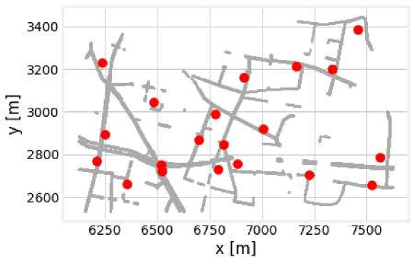
Figure 2: Road topology, with red dots corresponding to RSUs.

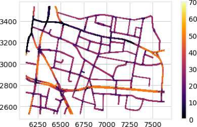
(a)

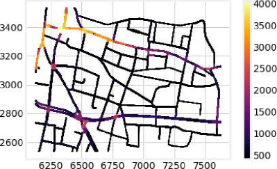
(b)

Figure 3: Speed (a) and density (b) of vehicles at different location of the trace we use. The scale is in km/h in (a) and vehicles per square kilometers in (b); darker colors correspond to higher values.

This section describes our reference network scenario and the architecture of the virtualized bachkaul under study. Specifically, Sec. 3.1 details the real-world, large-scale scenario we seek to emulate, and its traffic and demand patterns. Then, in Sec. 3.2, we discuss how we emulate such a scenario using Mininet and Docker, as well as the applications we run within each emulated node. Finally, Sec. 3.3 describes how the communication on the radio link is simulated and how the resulting delay is accounted for in the network emulations.

3.1 Reference scenario

As mentioned earlier, the beacons include the position, speed and direction of the vehicle sending them. In our experiments, this information is obtained from the mobility trace presented in [13]. Therein, the authors combine a $1.5\times 1$ km² section of the real-world road topology of the city of Ingolstadt (Germany), depicted in Fig. 2, and realistic vehicular mobility obtained with the SUMO simulator [14]. Ingolstadt is a medium-sized city in the Munich metropolitan area; the inner city includes a mixture of narrow streets and wider, multi-lane roads, as it is common in urban areas throughout the world. Taking it as our main reference scenario allows us to easily generalize the main indications in which we are interested, to other cities and countries. It is also worth stressing that, in Sec. 5.3, we check to which extent considering another road topology and user mobility impacts our results.

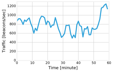
(a)

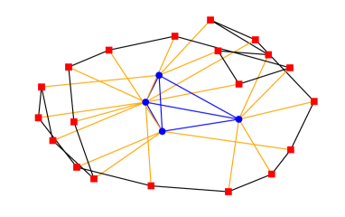
(b)

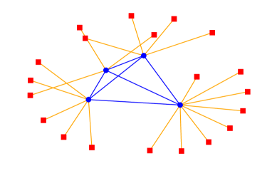
(c)

Figure 4: Evolution of the traffic load over time (a); mesh-like (b) and star-like (c) network topologies, with red dots corresponding to RSUs and blue ones representing core switches.

In SUMO, vehicles are associated with a random source and destination locations on the edge of the road topology, and move from the former to the latter following the fastest (not necessarily the shortest) route. The mobility simulated by SUMO accounts for such factors as speed limits on different roads, the number and direction of lanes therein, vehicles altering their course to overtake and/or avoid incidents, and traffic lights. The resulting average and maximum speeds are 12.9 and 70.1 km/h respectively, while the average acceleration and deceleration values are 0.44 and 0.33 m/s². The maximum deceleration, corresponding to vehicles violently braking to avoid an obstacle, is 128.8 m/s². Both the speed and density of vehicles in the trace, depicted in Fig. 3(a) and Fig. 3(b), respectively, closely reproduce their real-world counterparts, with higher speeds along the main thoroughfares and higher densities around busy intersections.

The topology also includes 20 RSUs, represented by red dots in Fig. 2. RSUs are placed at the busiest road intersections, so as to cover a large set of vehicles. Specifically, we employ the following greedy procedure for RSU placement:

1. we consider a set of candidate locations;

2. for each candidate location, we compute a score, corresponding to the number of vehicles passing through it;

3. we place one RSU at the candidate location with the highest score;

4. we subtract the newly-covered vehicles from the scores of all candidate locations;

5. we repeat steps 3–4 until all RSUs are placed.

While more complex deployment strategies exist [15, 16], they are typically tailored around one specific application, while we are interested in modeling general-purpose vehicular networks supporting several services.

RSU coverage and interference are computed according to the model presented in [13], which results in a maximum coverage radius of 255 meters. On average, successfully-transmitted beacons travel 123 meters between vehicles and RSUs.

At any given time, there are between 1,000 and 2,500 vehicles present in the topology, a value representative of the morning and afternoon peak times (i.e., 8:00-8:30 am and 5:00-5:30 pm, respectively.) All vehicles send a beacon each second [3, 4], which yields the traffic demand depicted in Fig. 4(a). Notice that, while vehicles not covered by an RSU still generate beacons, those beacons do not reach the collision detectors, and thus are not accounted for in Fig. 4(a).

Our real-world trace contains no information on the network topology, i.e., how the RSUs are connected with each other and with the core network. Network topologies can have a substantial impact on performance; intuitively, we can expect sparser topology to put a higher stress on switches – and the controller controlling them. We study two such topologies, represented in Fig. 4(b) and Fig. 4(c) respectively. In both topologies, we create one switch for each RSU (red dots in the figure), and add four core-level switches (blue dots). In the mesh-like topology (Fig. 4(b)), we then connect:

• the core switches in a mesh (blue links in Fig. 4(b));

• each RSU switch to the two closest core switches (orange links in Fig. 4(b));

• each RSU switch is also connected to the two closest RSU switches (black links in Fig. 4(b)).

The star-like topology, shown in Fig. 4(c), is less connected. With respect the mesh-like topology:

• RSU switches are only connected to the closest core switch;

• there are no links between RSU switches.

In our experiments, the number and location of collision detectors is not determined a priori: collision detectors can be placed at any RSU or core switches. We refine these decisions through the greedy, iterative process described later in Sec. 4. Furthermore, we remark that the above 24 switches are controlled by a single SDN controller.

3.2 Mininet network structure

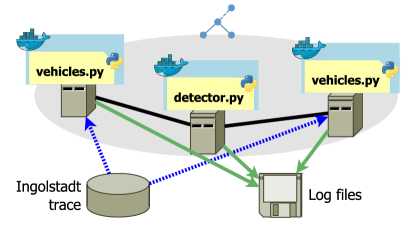
Figure 5: Our network architecture. A Mininet network (the gray area) contains several Mininet hosts (switches are not represented for simplicity). Within each host, we run a Docker container, and within the container one of two Python scripts: vehicles.py emulates the vehicles passing by an RSU, while detector.py is a collision detector. Mobility information is read from the Ingolstadt trace described in Sec. 3.1. Both collision detectors and vehicles store detailed log information, which is later used to obtain the performance metrics presented in Sec. 5.

The basic structure of our network is summarized in Fig. 5. We have a Mininet emulated network, including:

• one OpenVSwitch controller, bundled with Mininet;

• one switch for each of the 20 RSUs and four extra core switches;

• one host per RSU;

• one host per collision detector.

Recall that switches are connected as described in Fig. 4(b)–Fig. 4(c). For Mininet-emulated links, we conservatively keep the default bandwidth of 1 Gbit/s and the default latency of 0.12 ms. Within each Mininet host, we run a Docker container, and within each container we run a Python program, which depends on the type of host (either a RSU or a collision detector host).

As far as RSU hosts are concerned, we connect each host to the corresponding RSU switch, and run the vehicles.py script, which represents the vehicles under the RSU (see Fig. 5), on the host. The vehicles.py script is in charge of:

• reading the mobility information from the real-world trace from the city of Ingolstadt, described in Sec. 3.1;

• generating the beacons carrying the above mobility information, and transmitting them to the collision detector;

• receiving the replies from the collision detector, and logging the elapsed time.

The collision detector program, detector.py runs within the collision detector hosts, and:

• receives beacons sent by the vehicles;

• detects collisions, by running Alg. 1 described earlier;

• sends collision reports as appropriate;

• logs the time it took to process each beacon.

Notice that, for each beacon, we log two times: the delay perceived by the vehicle, i.e., the time elapsed between sending the beacon and receiving the reply, and the time used by the collision detector to actually process the beacon. The difference between these times is the network delay, i.e., the time packets spend traveling from the vehicle to the collision detector and vice versa within the emulated network.

Each beacon/reply consists of a single UDP packet. Also, we stress that, owing to the dynamic nature of vehicular scenarios, there are no persistent connections between vehicles and collision detectors.

Controllers. SDN networks include a controller, a software program that determines the forwarding behavior of switches. In the simplest case:

• switches have a set of rules, determining how packets shall be treated (forward on a certain port, flood, discard…);

• upon receiving a packet that does not match any of the existing rules, switches will forward it to the controller;

• based on the headers and/or payload of the packet, the controller will install one or more rules on the switch.

Being software programs, controllers can make switches behave in virtually any way. One of the simplest behaviors controllers can implement is the so-called learning switch: the controller observes from which port of each switch packets coming from a certain host are received, and “learns” that future packets directed to that host shall be forwarded on the same port.

In our experiments, we compare two SDN controllers, both implementing the learning switch behavior: Pox and Floodlight. Both are popular, actively maintained open-source projects; however, they have slightly different goals and scopes. Pox [7] is written in Python and is based on an older project called NOX; it aims at providing a simple, object-oriented interface to OpenFlow, and is often used in research projects. Floodlight [8] is written in Java, and its community tends to focus on providing high performance, configurability (e.g., through a REST API) and manageability (through web-based GUIs). Both controllers are vastly more capable than it is needed for our scenario; however, we are interested to see whether they provide us with different trade-offs between performance and complexity (hence, energy consumption).

3.3 Wireless simulations

Since Mininet does not support the emulation of wireless networks, we cannot use it to study the delay incurred by beacons when going from vehicles to RSUs. Instead, we resort to simulations, based on the popular, open-source simulator ns-3 [17]. ns-3 includes a detailed WAVE model, reproducing both its MAC layer and multi-channel coordination mechanism.

As specified by the IEEE 1609.4 standard, we set the control and service channels (CCH and SCH, respectively) to take 50 ms each. All beacons are transmitted on the CCH and all communication happens on the 5.9-GHz band, with a channel bandwidth of 10 MHz. We perform our simulations as follows:

• we take the position of RSUs and the mobility of vehicles from the Ingolstadt trace described in Sec. 3.1, so as to guarantee the consistency between simulation and emulation;

• as in the emulated scenario, vehicles transmit a beacon every second;

• we measure the time it takes for beacons to reach the RSUs.

We then add the beacon-specific delays we obtain from the simulation to our emulation results, thus being able to account for the radio link contribution to the total latency.

4 Collision detector placement

As mentioned in Sec. 3.1, a key feature of our scenario is that any number of collision detectors can be attached at any point of the network topologies described in Fig. 4(b)–Fig. 4(c). This reflects the increased flexibility offered by the network function virtualization (NFV), where any network node can run (virtually) any program. We therefore have to establish (i) how many collision detectors we need in our network in order to ensure that a sufficiently high fraction of beacons are served within the deadline set by the application, and (ii) where in the network topology these detectors should be placed.

Assuming we want at most one detector per node, this translates into deciding, for each of the 24 network nodes depicted in Fig. 4(b)–Fig. 4(c) (20 RSUs plus 4 core switches), whether or not we place a detector therein. This produces a total of $2^{24}\approx 16\cdot 10^{6}$ combinations. Recall that, because we are emulating networks, as opposed to simulating them, testing one combination with the one-hour trace we use also takes one hour. Thus, testing all possible combinations is clearly impractical. A popular and effective approach is coupling network simulation (or emulation, in our case) with stochastic optimization algorithms, as done in [18]. Intuitively, stochastic optimization techniques [19] are based on evaluating the performance (fitness) of a set of randomly-generated solutions, combining the most promising ones into new solutions to evaluate, and repeating the process until convergence is reached. They have been shown [20] to find optimal or quasi-optimal solutions after testing a very limited number of alternatives, i.e., performing a very limited number of simulations (or emulations in our case).

Considering that optimization is not the focus of our study, we further simplify the collision detector placement, and follow the greedy refinement procedure below. Given the number $n$ of detectors to deploy, we:

1. start by placing the detectors at randomly chosen nodes;

2. emulate the configuration thus obtained, and consider, for each RSU, the success fraction, i.e., the fraction of beacons originated within the RSU coverage for which a reply from the collision detector is received within the deadline;

3. for each switch (either RSU or core switch), compute the success fraction corresponding to the neighboring RSUs;

4. move a detector from the switch with the highest success fraction (among those having a detector) to the switch with the lowest success fraction (among those not having a detector);

5. if the configuration has been already tested, move a randomly-chosen detector to a randomly-chosen switch;

6. go to step 2.

Notice how the random changes in step 5 are equivalent to the mutation step in genetic [19] and simulated annealing [20] algorithms. Furthermore, a desirable aspect of our procedure is that there are no meta-parameters that need tweaking: this simplifies our study, and guarantees that none of the results we will observe is an artifact of a specific parameter setting.

Although we cannot formally prove any property in this respect, we consistently observed the greedy refinement procedure outlined above to converge in twenty to thirty iterations, corresponding to an emulation time of roughly one day. Additionally, the runs for different values of $n$ are independent and can be run in parallel: indeed, all the results we show in Sec. 5 can be obtained over a weekend.

5 Numerical results

For our performance evaluation, we set the deadline by which replies shall be received to 20 ms, as suggested by the real-world motorway trial [21]. Then, in Sec. 5.1, we change the number $n$ of detectors between 1 and 5 and, for each value of $n$, we study the overall detection performance, e.g., the fraction of successfully processed beacons, along with the associated delay and energy consumption. In Sec. 5.2 we investigate how changing the core network topology or the SDN controller influences the system performance and energy consumption. Finally, Sec. 5.3 presents some results obtained using a different road topology and user mobility trace.

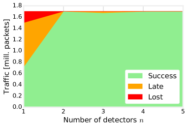
(a)

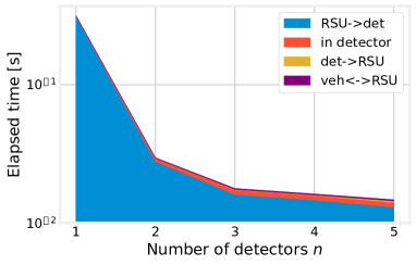
(b)

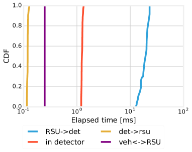
(c)

Figure 6: Default scenario. (a): Number of successfully processed, delayed and lost beacons as a function of the number $n$ of detectors. (b): Breakdown of the delay in its components. (c): Distribution of the delay components when $n=2$.

5.1 Default scenario

In the following, we consider a default scenario, where:

• the road topology and user mobility are modeled as described in Sec. 3.1;

• we use the star-like core network topology depicted in Fig. 4(c);

• all switches are controlled by a Pox [7] SDN controller.

The most basic aspect we are interested in is the effectiveness of our collision detection system. Out of all the beacons sent by vehicles, we need to know how many are (i) successfully processed, i.e., receive a response within the set deadline; (ii) late, i.e., receive a response but later than the deadline; (iii) lost, i.e., never receive a response. These three cases are represented by green, yellow and red areas in Fig. 6(a) respectively.

Fig. 6(a) shows that, as long as there is more than one collision detector deployed in the network, virtually all beacons can be processed within the deadline. Only in the case $n=1$ we can observe a small number of lost beacons, and a substantial fraction of beacons that are replied to too late. Bearing in mind that we are taking into account a medium-sized European city under congested traffic conditions, our results suggest that the task of collision detection can indeed be successfully tackled through a vehicular network based on SDN/NFV.

Fig. 6(b) breaks the delay down into four components:

• the time to reach the detector from the RSU (labeled as RSU->det);

• the processing time within the detector, e.g., to run Alg. 1 (labeled as in_detector);

• the time to reach RSU from the detector (labeled as det->RSU);

• the time beacons and alerts spend in the air (labeled as veh<->RSU).

While we might expect these components to be roughly equivalent, Fig. 6(b) shows the opposite: the time to transfer the beacons from the RSUs to the detector outweighs all other components; as confirmed by the CDFs in Fig. 6(c), the difference is of almost two orders of magnitude. Interestingly, Fig. 6(c) also shows that the time needed by data to travel in the opposite direction, i.e., from the detector to the RSUs, is much shorter, even shorter than the processing time at the detector.

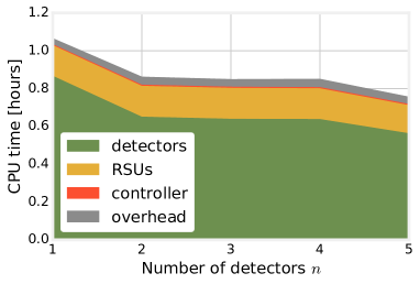
(a)

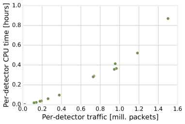
(b)

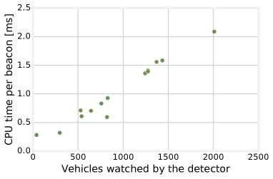
(c)

Figure 7: Default scenario. (a): How much CPU time is consumed by the detector.py script simulating detectors (yellow), vehicle.py scripts simulating vehicles (green), the pox controller (red), Mininet and Docker overhead (gray), for each value of $n$. (b): Link between the number of beacons processed by a detector and the CPU time it consumes. (c): Link between the number of vehicles watched by each detector and its per-beacon CPU consumption.

This is due to the fact that, while most packets are directly processed at the switches, some – those that do not match the forwarding rules currently stored at the switch – are forwarded to the SDN controller, which substantially increases the amount of time needed to forward the packets. Indeed, the OpenVSwitch virtual switches first cache the forwarding instructions of the SDN controller for some time (which explains why the replies going from the detectors to the RSUs are much less likely to be forwarded to the controller again) and then purge them after a timeout, in order to avoid keeping stale routes.

This unexpected effect serves us as a reminder that SDN does not represent a drop-in replacement for traditional networks, and special attention ought to be devoted to the interaction between nodes of the data plane and controllers. At the same time, it further highlights how network emulation is an excellent tool to study SDN networks.

In Fig. 7, we move to energy consumption. Specifically, we use the CPU time logged by the different components of our system as a proxy for the actual energy they consume; this is in line with such recent works as [22], that identify an almost-linear relationship between CPU utilization and energy consumption.

Fig. 7(a) shows the CPU time logged by detectors (i.e., the detector.py instances), RSUs (i.e., vehicle.py instances) and controllers, as a function of the number $n$ of detectors. It also represents the overhead due to Mininet, Docker, and the virtual machine Mininet runs on (gray area in the plot). Recall that our tests last one hour, and the total consumed CPU time can exceed that because different components, e.g., two collision detectors, can use different CPUs at the same time.

A first thing we can observe is that collision detectors consume most of the CPU time; indeed, when $n=1$, the detector is active for more than 50 minutes. rsu.py scripts also consume a fair amount of CPU, due to their manifold role of sending the beacons, receiving the replies, and logging the elapsed times. The CPU time consumed by the detector, on the other hand, is almost negligible, amounting to barely 30 seconds. This confirms that SDN controllers per se do not substantially increase the energy consumption of the networks they belong to, and SDN itself is a suitable technology to use in energy-constrained network scenarios.

Another interesting aspect we can learn from Fig. 7(a) is that the total CPU time consumed decreases as $n$ grows, even as the system performance (Fig. 6(a)) increases. To understand the reason for this, we show in Fig. 7(b) the CPU time consumed by each detector as a function of the number of beacons it has to process throughout the whole simulation. There are a total of fifteen points in Fig. 7(b): one for the single detector deployed when $n=1$ (the topmost one, corresponding to the CPU time consumption we see in the leftmost part of Fig. 7(a)), two for the two detectors deployed when $n=2$, and so on. We can clearly see that, the more beacons a detector has to process, the more CPU time it will consume.

Fig. 7(b) is not especially surprising: detectors basically run Alg. 1 every time they receive a beacon, so it stands to reason that doing that more often translates into a higher CPU consumption. More interestingly, Fig. 7(c) correlates the per beacon CPU consumption with the number of vehicles each detector has within its coverage area. We can observe an almost linear correlation between the two. It tells us that having more vehicles to deal with not only means that collision detectors need to process more beacons, but also that each beacon takes longer to process. The reason lies in the structure of Alg. 1 itself: in Line 4, we loop over all (recent) beacons received by other vehicles, and the number thereof directly depends upon the number of vehicles the detector has to watch.

Summary. In our default scenario (star-like topology as depicted in Fig. 4(c), Pox controller), any value of $n$ greater than one guarantees that virtually all beacons are processed successfully (Fig. 6(a)). Having to send some packets to the SDN controller is the main source of delay (Fig. 6(b), Fig. 6(c)), and collision detectors consume most of the CPU time (Fig. 7(a)), and thus most of the energy. Such a consumption increases with the total traffic each detector has to process (Fig. 7(b)), as well as the number of vehicles it has to watch (Fig. 7(c)). This suggests that improved, more efficient collision detection algorithms are a worthwhile direction to follow in order to reduce the energy consumption of vehicular safety networks.

5.2 Alternative backhaul topology and detector

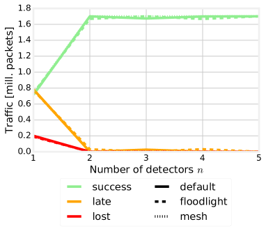
(a)

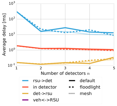
(b)

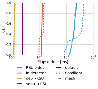
(c)

Figure 8: Mesh-like topology (“mesh”) and Floodlight controller (“floodlight”) scenarios. (a): Number of successfully processed, delayed and lost beacons as a function of the number $n$ of detectors. (b): Breakdown of the delay in its components. (c): Distribution of the delay components when $n=2$.

In the following, we maintain the same road topology and mobility trace as considered before, and address two alternative backhaul scenarios:

• one labeled “mesh”, where we replace the star-like network topology depicted in Fig. 4(c) with the mesh-like one depicted in Fig. 4(b);

• one labeled “floodlight”, where we replace the Pox controller with the Floodlight [8] one.

Notice that we are interested in studying the effect of these two changes individually; therefore, in the “mesh” scenario we use the same Pox controller as in the default one, and in the “floodlight” scenario we use the same star-like topology as in the default one.

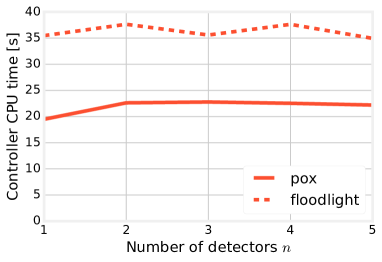
Figure 9: CPU time used by Pox (solid lines) and Floodlight (dashed lines) controllers, as $n$ changes.

Fig. 8(a) shows that the performance is virtually the same in all scenarios. Intuitively, this tells us that the collision detection system we devised is robust to changes in the network topology and type of SDN controller. There are, however, some slight but significant differences in the delay: specifically, we can see from Fig. 8(b) that using the mesh-like network topology corresponds to shorter delays, which again makes sense as in that case individual switches tend to be less loaded.

More interestingly, in Fig. 8(c) we see that the Floodlight controller is associated with a stronger variability in the delay, especially for the packets sent from detectors to RSUs: some are processed very quickly, while others take substantially longer than with the Pox controller. Furthermore, this also affects the time spent by packets in the controller (red lines in Fig. 8(c)), whose variability increases as well. Indeed, as we observed earlier, the time it takes the detector to process a beacon depends on how many beacons the detector has received in the recent past, and that can change substantially if controller-induced delays are not constant.

Fig. 9 shows another difference between Pox and Floodlight controllers: the latter consumes substantially more CPU time than the former. Such a difference is due to the different language they use (Java programs tend to be heavier than their Python counterparts), and, to a greater extent, to Floodlight focusing on feature-richness over simplicity.

Summary. Using a different controller or a different network topology does not substantially change the system performance (Fig. 8(a)). However, a more connected topology translates into slightly shorter delays (Fig. 8(b)). Using the Floodlight controller in lieu of Pox yields a higher variance in packet processing delay (Fig. 8(c)), as well as higher CPU time consumption (Fig. 9).

5.3 Alternative road topology and mobility trace

We now consider a different trace, coming from German city of Cologne [23]. Similar to the Ingolstadt trace detailed in Sec. 3.1, it combines real-world topology with realistic vehicle mobility obtained through SUMO. The area covered by the trace is 2 $\times$ 2 km², and there are on average 2,410 vehicles, traveling at an average speed of 41.98 km/h. We place 20 RSUs on the topology, following the same greedy procedure as in the Ingolstadt case. Fig. 10(a) shows the road topology (in gray) and the location of RSUs (red dots).

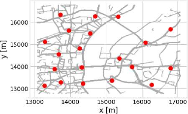
(a)

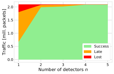
(b)

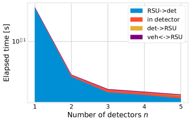
(c)

Figure 10: Cologne scenario. (a): road topology and RSUs location; (b): number of successfully processed, delayed and lost beacons as a function of the number $n$ of detectors; (c): breakdown of the delay in its components.

Fig. 10(b) summarizes the number of beacons that are processed successfully, delayed, or lost. We can observe that, in spite of the higher number of beacons (notice the y-scale in the plot), two detectors are sufficient to provide the collision detection service with a small number of delayed or lost beacons.

We can further confirm this by comparing Fig. 10(c) to Fig. 6(b). Both the overall delay and its components are very similar between the Ingolstadt and Cologne scenarios: the main difference lies in slightly longer delays in the collision detectors for the Cologne scenario (red area in Fig. 10(c)), due to the higher number of vehicles.

6 Related work

6.1 Collision detection

Collision detection for vehicular networks is a widely studied topic. Earlier works such as [24] focus on system architecture, e.g., the role of RSUs, while later ones address specific aspects such as countering shadowing effects [3] or evaluating competing systems [25]. In a recent twist, [26] advocates using smartphone data along with the beacons that vehicles periodically transmit.

Another significant aspect of collision detection systems is security. Indeed, beacons can be used by malicious attackers to reconstruct the vehicle position and/or trajectory [10, 11]. Anonymous beacons improve the situation [11]; however, they can be abused by vehicles providing false information [4] to hide their position to the authorities.

Compared to these works, the collision detection solution we present in Sec. 2 is remarkably simple. This is due to the fact that our focus is not on optimizing collision detection, but rather on assessing the ability of SDN/NFV-based networks to meet the strict latency constraints imposed by vehicular collision detection, and the resulting energy consumption.

6.2 SDN and NFV

Our work is also related to the wide area of software-defined networking and network function virtualization. In particular, the authors of the early work [27] envision a software-based implementation of next-generation cellular networks, where all types of network nodes, e.g., firewalls and gateways, are implemented through middleboxes, virtual machines running on general-purpose hardware. The concept of middleboxes is further generalized into virtual network functions (NFV) [28], capable of performing any task, including those usually carried out by ad hoc servers, e.g., video transcoding.

Enabled by SDN and NFV, mobile-edge computing (MEC) has been recently introduced [29] as a way to move “the cloud”, i.e., the servers processing mobile traffic, closer to users, thus reducing the latency and load of networks. Recent works have studied the radio techniques needed to enable MEC [30], its relationship to the Internet-of-things [31] and context-aware, next-generation networks [32].

Placing the VNFs and the servers hosting them within the cellular network is one of the most important MEC-related research question, the most popular approach being exact [33] and approximate [34, 35] optimization. When faced with the task of placing our collision detectors, we take the more straightforward approach of refining their positioning, as detailed in Sec. 4; indeed, for us the impact of different placement solutions on the resulting delay and energy consumption is more important than finding the utmost optimal solution.

7 Conclusion and future work

Collision detection is a prominent safety application of vehicular networks, having very strict delay requirements. In order to verify the compatibility of these requirements with SDN and NFV, we designed, implemented and emulated one such collision detection system using Mininet and Docker.

Using a real-world road topology and mobility trace, we found that a limited number of collision detectors can process the vast majority of beacons with acceptable delay. More importantly, we found that most of that delay comes from packets being sent to the SDN controller; this further highlights the importance of thoroughly testing SDN-based solutions before deploying them.

References

- [1] National Highway Traffic Safety Administration, Fatality Analysis Reporting System, https://www-fars.nhtsa.dot.gov/Main/index.aspx.
- [2] World Health Organization, Global status report on road safety, http://www.who.int/violence_injury_prevention/road_safety_status/2015/GSRRS2015_data/en/.
- [3] C. Sommer, S. Joerer, M. Segata, O. K. Tonguz, R. Lo Cigno, F. Dressler, How Shadowing Hurts Vehicular Communications and How Dynamic Beaconing Can Help, IEEE Transactions on Mobile Computing.
- [4] F. Malandrino, C. Borgiattino, C. Casetti, C. F. Chiasserini, M. Fiore, R. Sadao, Verification and Inference of Positions in Vehicular Networks through Anonymous Beaconing, IEEE Transactions on Mobile Computing.
- [5] NHTSA, U.S. DOT advances deployment of Connected Vehicle Technology to prevent hundreds of thousands of crashes, http://bit.ly/2hMmtSk.
- [6] N. Handigol, B. Heller, V. Jeyakumar, B. Lantz, N. McKeown, Reproducible Network Experiments Using Container-based Emulation, in: ACM CoNEXT, 2012.
- [7] The POX controller, https://github.com/noxrepo/pox.
- [8] The Floodlight controller, http://www.projectfloodlight.org/floodlight/.
- [9] Docker, http://docker.com.
- [10] S. Al-Shareeda, F. Özgüner, Preserving location privacy using an anonymous authentication dynamic mixing crowd, in: IEEE ITSC, 2016.
- [11] H. Artail, N. Abbani, A Pseudonym Management System to Achieve Anonymity in Vehicular Ad Hoc Networks, IEEE Transactions on Dependable and Secure Computing.
- [12] F. Gong, B. Gao, Q. Niu, An Algorithm for Rapidly Computing the Minimum Distance between Two Objects Collision Detection, in: 2008 Congress on Image and Signal Processing, 2008.
- [13] C. Sommer, D. Eckhoff, F. Dressler, IVC in cities: signal attenuation by buildings and how parked cars can improve the situation, IEEE Transactions on Mobile Computing.
- [14] DLR Institute, The SUMO Mobility Simulator, http://www.dlr.de/ts/en/desktopdefault.aspx/tabid-9883/16931_read-41000/.
- [15] F. Malandrino, C. Casetti, C.-F. Chiasserini, M. Fiore, Optimal content downloading in vehicular networks, IEEE Transactions on Mobile Computing 12 (7) (2013) 1377–1391.
- [16] Y. Liang, H. Liu, D. Rajan, Optimal placement and configuration of roadside units in vehicular networks, in: Vehicular Technology Conference (VTC Spring), 2012 IEEE 75th, 2012, pp. 1–6.
- [17] The ns-3 simulator, http://nsnam.org.
- [18] A. Hess, F. Malandrino, M. B. Reinhardt, C. Casetti, K. A. Hummel, J. M. Barceló-Ordinas, Optimal deployment of charging stations for electric vehicular networks, in: ACM CoNEXT UrbaNe Workshop, 2012.
- [19] K. Deb, A. Pratap, S. Agarwal, T. Meyarivan, A fast and elitist multiobjective genetic algorithm: NSGA-II, IEEE Transactions on Evolutionary Computation.
- [20] E. Aarts, J. Korst, W. Michiels, Simulated Annealing, Springer US, Boston, MA, 2014.
- [21] Nokia Networks, Continental, Deutsche Telekom, Fraunhofer ESK, and Nokia Networks Showcase First Safety Applications at Digital A9 Motorway Test Bed , http://www.prnewswire.com/news-releases/continental-deutsche-telekom-fraunhofer-esk-and-nokia-networks-showcase-first-safety-applications-at-digital-a9-motorway-test-bed-543728312.html.
- [22] B. Krishnan, H. Amur, A. Gavrilovska, K. Schwan, VM power metering: feasibility and challenges, ACM SIGMETRICS Performance Evaluation Review.
- [23] D. Naboulsi, M. Fiore, On the instantaneous topology of a large-scale urban vehicular network: The Cologne case, in: ACM MobiHoc, 2013.
- [24] F. J. Martinez, C. K. Toh, J. C. Cano, C. T. Calafate, P. Manzoni, Emergency Services in Future Intelligent Transportation Systems Based on Vehicular Communication Networks, IEEE Intelligent Transportation Systems Magazine.
- [25] S. Joerer, M. Segata, B. Bloessl, R. L. Cigno, C. Sommer, F. Dressler, A Vehicular Networking Perspective on Estimating Vehicle Collision Probability at Intersections, IEEE Transactions on Vehicular Technology.
- [26] H. Sharma, R. K. Reddy, A. Karthik, S-CarCrash: Real-time crash detection analysis and emergency alert using smartphone, in: IEEE ICCVE, 2016.
- [27] X. Jin, L. E. Li, L. Vanbever, J. Rexford, Softcell: Scalable and flexible cellular core network architecture, in: ACM CoNEXT, 2013.
- [28] ETSI, Mobile edge computing white ppaer, http://www.etsi.org/technologies-clusters/technologies/mobile-edge-computing.
- [29] Cisco, Transform Data into Action at the Network Edge (2015).
- [30] S. Sardellitti, G. Scutari, S. Barbarossa, Joint Optimization of Radio and Computational Resources for Multicell Mobile-Edge Computing, IEEE Transactions on Signal and Information Processing over Networks.
- [31] F. Bonomi, R. Milito, J. Zhu, S. Addepalli, Fog Computing and Its Role in the Internet of Things, in: Proceedings of the First Edition of the MCC Workshop on Mobile Cloud Computing, 2012.
- [32] S. Nunna, A. Kousaridas, M. Ibrahim, M. Dillinger, C. Thuemmler, H. Feussner, A. Schneider, Enabling real-time context-aware collaboration through 5g and mobile edge computing, in: ITNG, 2015.
- [33] N. Gazit, F. Malandrino, D. Hay, Coopetition between network operators and content providers in SDN/NFV core networks, in: IEEE INFOCOM SWFAN Workshop, 2016.
- [34] R. Cohen, L. Lewin-Eytan, J. S. Naor, D. Raz, Near optimal placement of virtual network functions, in: IEEE INFOCOM, 2015.
- [35] J. Cao, Y. Zhang, W. An, X. Chen, Y. Han, J. Sun, VNF Placement in Hybrid NFV Environment: Modeling and Genetic Algorithms, in: IEEE ICPADS.