A Connection Between Time Domain Model Order Reduction and Moment Matching for LTI Systems

Abstract

We investigate the time domain model order reduction (MOR) framework using general orthogonal polynomials by Jiang and Chen [1] and extend their idea by exploiting the structure of the corresponding linear system of equations. Identifying an equivalent Sylvester equation, we show a connection to a rational Krylov subspace, and thus to moment matching. This theoretical link between the MOR techniques is illustrated by three numerical examples. For linear time-invariant systems, the link also motivates that the time domain approach can be at best as accurate as moment matching, since the expansion points are fixed by the choice of the polynomial basis, while in moment matching they can be adapted to the system.

1 Introduction

Various mathematical and physical processes can be modeled as linear time-invariant (LTI) input-output systems

$$\begin{split}E\dot{x}(t)&=Ax(t)+Bu(t),\\ y(t)&=Cx(t),\end{split}$$ (1)

where $E,A\in\mathbb{R}^{n\times n}$ are sparse matrices, $B\in\mathbb{R}^{n\times p}$ and $C\in\mathbb{R}^{q\times n}$ are input and output matrices, respectively, $x(t)\in\mathbb{R}^{n}$ is the state vector, $u(t)\in\mathbb{R}^{p}$ is the input vector, $y(t)\in\mathbb{R}^{q}$ is the output vector and $t\in\mathbb{R}$ represents time.

Since the order of the LTI system (1) is often huge $n\gg 10^{3}$, a numerical simulation might be too expensive or even impossible, caused by immense computational time and memory requirements. Nevertheless, the input-output behavior of (1) can be computed fast and accurately if the given system is reduced to a system

$$\begin{split}E_{r}\dot{x}_{r}(t)&=A_{r}x_{r}(t)+B_{r}u(t),\\ y_{r}(t)&=C_{r}x_{r}(t),\end{split}$$ (2)

that approximates the dynamic behavior of (1), but $E_{r},A_{r}\in\mathbb{R}^{r\times r}$, $B_{r}\in\mathbb{R}^{r\times p}$, $C_{r}\in\mathbb{R}^{q\times r}$, $x_{r}(t)\in\mathbb{R}^{r}$, $y_{r}(t)\in\mathbb{R}^{q}$ with the reduced order $r\ll n$.

The aim of MOR is to approximate a system (1) with a huge order $n$ by a system (2) with a much smaller order $r$, such that structural properties are preserved and the approximation error $y(t)-y_{r}(t)$ over a given time interval $[t_{0},t_{f}]$, or the error of the transfer functions $G(s)-G_{r}(s)$ over a frequency range $[s_{0},s_{1}]$, is small.

Transfer functions describe the relation between input and output in frequency domain. For (1), (2) with zero initial states and an evaluation point $s$ in frequency domain, these are given by

$$G(s) =C(sE-A)^{-1}B,$$ (3)

$$G_{r}(s) =C_{r}(sE_{r}-A_{r})^{-1}B_{r}.$$ (4)

There exist numerous MOR approaches. $\mathcal{H}_{2}$ optimal MOR techniques like the iterative rational Krylov algorithm (IRKA) (see, e.g. [2]) or the two-sided iteration algorithm (TSIA) (see, e.g. [3]) measure their approximation error $\epsilon_{2}$ in the $\mathcal{H}_{2}$ system norm (see, e.g. [4, Chapter 5])

$$\epsilon_{2}\coloneqq\|G(s)-G_{r}(s)\|_{\mathcal{H}_{2}}.$$

These techniques are just two types of projection based MOR methods. There, the system (1) is reduced using so-called projection matrices $V,W\in\mathbb{R}^{n\times r}$ that map the matrices $E,A,B$ and $C$ onto a subspace approximating the space of the state vector $x(t)$. The reduced system is given as

$$\begin{split}\underbrace{W^{T}EV}_{E_{r}}\dot{x}_{r}(t)&=\underbrace{W^{T}AV}_{A_{r}}x_{r}(t)+\underbrace{W^{T}B}_{B_{r}}u(t),\\ y_{r}(t)&=\underbrace{CV}_{C_{r}}x_{r}(t),\end{split}$$ (5)

where $x(t)\approx Vx_{r}(t)$. A more simple example for projection methods is moment matching, where $V$ and $W$ are computed to approximate the moments of the transfer function. This method and its relevant properties are repeated in Section 4.1. It represents one step in the procedure behind the IRKA iteration.

Also the balanced truncation technique falls into the class of projection based reduction methods. Its error $\epsilon_{\infty}$ is measured in the $\mathcal{H}_{\infty}$ norm (see, e.g. [4, Chapter 5])

$$\epsilon_{\infty}\coloneqq\|G(s)-G_{r}(s)\|_{\mathcal{H}_{\infty}}.$$

Applying this method, the system (1) is first balanced, i.e. the observability and controllability Gramians $P_{O}$ and $P_{C}$, given as the solutions of two Lyapunov equations

$$A^{T}P_{O}E+E^{T}P_{O}A =-C^{T}C,$$

$$AP_{C}E^{T}+EP_{C}A^{T} =-BB^{T},$$

are made equal and diagonal, such that $P_{O}=P_{C}=\text{diag}(\sigma_{1}\cdots\sigma_{n})$ and $\sigma_{1}\geq\cdots\geq\sigma_{n}>0$ are the systems invariant Hankel singular values (HSVs). The discardable portions are identified and truncated according to the magnitude of the HSVs. More details about this method can be found, e.g. in [4, Chapter $7$].

The above MOR techniques are motivated and derived by frequency domain considerations.

In contrast to that, we next review the idea of Jiang and Chen [1] presenting a time domain MOR framework based on orthogonal polynomials. In this paper we only consider single-input single-output (SISO) systems, i.e. $p=q=1$ in (1) to simplify the notation. Drawbacks of this method are the dependence of the reduced order model (ROM) on the input $u(t)$ and the initial state $x(t_{0})=x_{0}$.

The dependence on the input can be neglected, since we will see that piecewise constant controls, which are the most important ones in practical applications anyway, allow for a joint ROM to exist. However, a ROM depending on the initial state is undesirable since the reduced system needs to be recomputed for each initial state or ROMs need to be stored for all possible initial values.

Frequency domain based model reduction methods, such as balanced truncation or moment matching, assume $x(t_{0})=\left[0\ \cdots\ 0\right]^{T}=:~{}\mathbb{O}_{n,1}\in\mathbb{R}^{n}$, in the first place, in order to avoid additional terms in the transfer function representation (3). For the comparison, we will do the same in the time domain case in the following.

The remainder of this paper is organized as follows. The time domain MOR approach based on general orthogonal polynomials by Jiang and Chen [1] is introduced in Section 2. In Section 3, the structure of the resulting linear system of equations is exploited to derive an equivalent Sylvester equation. Further a slight variation of the approach is discussed that eliminates the initial condition in the case it is assumed to be zero, which also simplifies the structure of the coefficients in the Sylvester equation. Since we want to show a connection to moment matching, we briefly introduce this Krylov subspace method in Section 4 concluding with an important equivalence to the approaches of Section 3. Still, the additional freedom in the choice of the coefficients in the Sylvester equation makes moment matching theoretically more flexible and better adaptable to the original system under investigation. Numerical examples illustrated in Section 5 demonstrate this advantage. Concluding remarks are given in Section 6.

2 Time Domain MOR Based on Orthogonal Polynomials (TDMOR)

As already mentioned above, we restrict ourselves to SISO systems, i.e. $p=q=1$.

The framework in [1] uses $W=V$ in (5) and obtains the projection matrix $V\in\mathbb{R}^{n\times r}$ from the vector valued coefficients in series expansions of the state and input, sampling their time dependence via orthogonal polynomials [5, Chapter 22].

The key property of orthogonal polynomials for the derivation of the framework in [1] is given by the following theorem.

Theorem 2.1 (Differential recurrence formula, e.g. [6, Section $2.15$]).

For three subsequent orthogonal polynomials $g_{i}(t)$ ($i\in\mathbb{N}_{0}$) holds

$$g_{n}(t) =\alpha_{n}\dot{g}_{n+1}(t)+\beta_{n}\dot{g}_{n}(t)+\gamma_{n}\dot{g}_{n-1}(t),\quad\forall n\in\mathbb{N},$$

where $\alpha_{n},\beta_{n}$ and $\gamma_{n}$ are differential recurrence coefficients. A list of such coefficients for selected families can be found in Table 2.

Differential recurrence coefficients polynomial class $\alpha_{i}$ $\beta_{i}$ $\gamma_{i}$ Chebychev-1 $\frac{1}{2i+2}$ 0 $-\frac{1}{2i-2}$ Chebychev-2 $\frac{1}{2i+2}$ 0 $-\frac{1}{2i+2}$ Hermite $\frac{1}{2i+2}$ 0 0 Jacobi $(a,b>-1)$ $\frac{2(a+b+i+1)}{(a+b+2i+2)(a+b+2i+1)}$ $\frac{2(a-b)}{(a+b+2i)(a+b+2i+2)}$ $-\frac{2(a+i)(b+i)}{(a+b+2i+1)(a+b+2i)(a+b+i)}$ Laguerre -1 1 0 Legendre $\frac{1}{2i+1}$ 0 $-\frac{1}{2i+1}$

We restrict our considerations to the polynomials investigated in [1]. Other polynomials fulfilling Theorem 2.1 are for instance the Gegenbauer polynomials, a generalization of the Legendre polynomials (see, e.g. [6, Section $2.11$].

The following repeats some of the details of the derivation in [1]. First, the state, the initial condition and the input vector are approximated by the following truncated series expansions:

$$x(t) \approx x_{r}(t) = \sum_{i=0}^{r-1}v_{i}g_{i}(t),$$ (6)

$$x_{0}=x(t_{0}) \approx x_{r}(t_{0}) = \sum_{i=0}^{r-1}v_{i}g_{i}(t_{0}),$$ (7)

$$u(t) \approx u_{r}(t) = \sum_{i=1}^{r-1}w_{i}\dot{g}_{i}(t),$$ (8)

where $v_{i}\in\mathbb{R}^{n}$ and $w_{i}\in\mathbb{R}$ are weights determining the subspace $\operatorname{span}\!\left\{V\right\}$ and $g_{i}(t)$ are orthogonal polynomials representing the time dependence. Note, that the open literature provides no information about the remainder terms in (6)-(8). Thus, the estimation of approximation errors, and resulting model reduction errors, is at best difficult.

The approximations of the state (6) and the input (8) are inserted into the state equation of (1) and using Theorem 2.1, one obtains an expression that only depends on $\dot{g}_{i}(t)$, since $g_{0}$ is always constant:

$$B\left(\sum_{i=1}^{r-1}w_{i}\dot{g}_{i}(t)\right)= \sum_{i=1}^{r-1}\left(E-\beta_{i}A\right)v_{i}\dot{g}_{i}(t)-Av_{0}g_{0}(t)-\sum_{i=2}^{r}\alpha_{i-1}Av_{i-1}\dot{g}_{i}(t)-$$

$$-\sum_{i=1}^{r-2}\gamma_{i+1}Av_{i+1}\dot{g}_{i}(t).$$

A comparison of coefficients leads to the huge $(nr\times nr)$ linear system of equations $Hv=f$ presented in equation (9), where the approximation of the initial state (7) is only required to obtain a square matrix

$$\begin{bmatrix}g_{0}(t_{0})I_{n}&g_{1}(t_{0})I_{n}&g_{2}(t_{0})I_{n}&g_{3}(t_{0})I_{n}&\cdots&g_{r-1}(t_{0})I_{n}\\ -\frac{g_{0}(t)}{\dot{g}_{1}(t)}A&E-\beta_{1}A&-\gamma_{2}A&&&\\ &-\alpha_{1}A&E-\beta_{2}A&-\gamma_{3}A&&\\ &&\ddots&\ddots&\ddots&\\ &&&-\alpha_{r-3}A&E-\beta_{r-2}A&-\gamma_{r-1}A\\ &&&&-\alpha_{r-2}A&E-\beta_{r-1}A\end{bmatrix}\begin{bmatrix}v_{0}\vphantom{g_{0}(t_{0})I_{n}}\\ v_{1}\vphantom{\frac{g_{0}(t)}{\dot{g}_{1}(t)}AE-\beta_{1}A}\\ v_{2}\vphantom{\gamma_{2}}\\ \vdots\vphantom{\ddots}\\ v_{r-2}\vphantom{\beta_{r-2}}\\ v_{r-1}\vphantom{\beta_{r-1}}\end{bmatrix}=\begin{bmatrix}\vphantom{g_{0}(t_{0})I_{n}}x_{0}\\ \vphantom{\frac{g_{0}(t)}{\dot{g}_{1}(t)}AE-\beta_{1}A}Bw_{1}\\ \vphantom{\gamma_{2}}Bw_{2}\\ \vdots\vphantom{\ddots}\\ \vphantom{\beta_{r-2}}Bw_{r-2}\\ \vphantom{\beta_{r-1}}Bw_{r-1}\end{bmatrix},$$ (9)

and $I_{n}$ denotes the $n$-dimensional identity matrix.

In [1] this linear system of equations, with matrix $H\in\mathbb{R}^{nr\times nr}$ and right hand side $f\in\mathbb{R}^{nr}$, is solved using an iterative algorithm. The solution vector $v\in\mathbb{R}^{nr}$ is then used to compute the projection matrix $V\in\mathbb{R}^{n\times r}$ by orthogonalizing the span of $\left[v_{1},\cdots,v_{r}\right]$. In the following context, we will call this method TDMOR.

Note that $H$ is not depending on time, since both $g_{0}$ and $\dot{g}_{1}$ are constant in time. Further, the matrix $H$ has a certain block-structure. We exploit this structure in the following section to derive an equivalent formulation and a more well-posed variation of this MOR method.

3 Structure Exploitation and a Slight Variation

3.1 Structure Exploitation (SYLTDMOR1)

We multiply the first equation in (9) by $A$ and obtain the following equivalent linear system of equations in Kronecker product (see, e.g. [7, Section $4.2$]) form

$$\left(\tilde{E}^{T}\otimes A+\tilde{A}^{T}\otimes E\right)v=\tilde{f}.$$

Here

$$\tilde{E}^{T} =\begin{bmatrix}g_{0}(t_{0})&g_{1}(t_{0})&g_{2}(t_{0})&g_{3}(t_{0})&\cdots&g_{r-1}(t_{0})\\ -\displaystyle\frac{g_{0}(t)}{\dot{g}_{1}(t)}&-\beta_{1}&-\gamma_{2}&&&\vphantom{\vdots}\\ &-\alpha_{1}&-\beta_{2}&-\gamma_{3}&&\\ &&\ddots&\ddots&\ddots&\\ &&&-\alpha_{r-3}&-\beta_{r-2}&-\gamma_{r-1}\\ &&&&-\alpha_{r-2}&-\beta_{r-1}\vphantom{\vdots}\end{bmatrix}\in\mathbb{R}^{r\times r},$$

$$\tilde{A}^{T} =\begin{bmatrix}\mathbb{O}_{1,1}&\mathbb{O}_{1,r-1}\\ \mathbb{O}_{r-1,1}&I_{r-1}\\ \end{bmatrix}\in\mathbb{R}^{r\times r},$$

$$\tilde{f} =\begin{bmatrix}(Ax_{0})^{T}&(Bw_{1})^{T}&\ldots&(Bw_{r-1})^{T}\end{bmatrix}^{T}\in\mathbb{R}^{nr}.$$

Using the equivalence

$$\left(B^{T}\otimes A\right)\text{vec}(X)=\text{vec}(C)\Leftrightarrow AXB=C,$$ (10)

(see, e.g. in [7, Section $4.3$]) we obtain a Sylvester equation

$$AV\tilde{E}+EV\tilde{A}=\tilde{F},$$ (11)

where $v=\text{vec}(V)$, $\tilde{f}=\text{vec}\left(\tilde{F}\right)$ and vec$(.)$ of a matrix $A\in\mathbb{R}^{m\times n}$ is defined as in

$$\text{vec}(A)=\begin{bmatrix}a_{1,1},\ldots,a_{m,1},a_{1,2},\ldots,a_{m,2},\ldots,a_{1,n},\ldots,a_{m,n}\end{bmatrix}^{T}$$

and is called a vectorization (see, e.g. [7, Section $4.2$]). A further orthogonalization of $V$ leads to the desired projection matrix. In the following, we will refer to this algorithm as SYLTDMOR1.

Note that the matrix pencil $(\tilde{A},\tilde{E})$ has at least one eigenvalue equal to zero caused by the structure of $\tilde{A}$, which arises from the initial state condition. Therefore the matrix $H$ in (9) is not invertible resulting in an infinite number of solutions and thus in a possibly infinite number of ROMs. Hence, this method is not well-posed and its solution not well-defined.

3.2 Variation of the Presented Algorithm (SYLTDMOR2)

In the approach of Jiang and Chen [1], the approximation of the initial state is only required to obtain a square matrix. As a conclusion of Section 3.1, this condition turned out to be linearly dependent anyway. Besides, a ROM depending on the initial state is not desirable.

In Section 5, we compare to the frequency domain methods, thus also here we fix the initial state to $x_{0}=x(t_{0})=\mathbb{O}_{n,1}$.

Doing so, we can neglect the constant polynomials $g_{0}(t)$ in the approximations (6). In order to keep an $r$ dimensional approximation, we shift the sums by 1. Using the same procedure as in Section 2, we end up with an ${nr\times nr}$ linear system of equations $\hat{H}\hat{v}=\hat{f}$. Rewriting it, again using the Kronecker product, we obtain

$$\left(\hat{E}^{T}\otimes A+\hat{A}^{T}\otimes E\right)\hat{v}=\hat{f},$$

where now

$$\hat{E}^{T} =-\begin{bmatrix}\beta_{1}&\gamma_{2}&&&\\ \alpha_{1}&\beta_{2}&\gamma_{3}&&\\ &\ddots&\ddots&\ddots&\\ &&\alpha_{r-2}&\beta_{r-1}&\gamma_{r}\\ &&&\alpha_{r-1}&\beta_{r}\end{bmatrix}\in\mathbb{R}^{r\times r},\qquad\hat{A}^{T}=I_{r},$$

$$\hat{v} =\begin{bmatrix}\hat{v}_{1}^{T}&\ldots&\hat{v}_{r}^{T}\end{bmatrix}\in\mathbb{R}^{nr},\qquad\hat{f}=\begin{bmatrix}\left(Bw_{1}\right)^{T}&\ldots&\left(Bw_{r}\right)^{T}\end{bmatrix}^{T}\in\mathbb{R}^{nr}.$$

Exploiting the equivalence (10) and the fact $\hat{A}=I_{r}$, the linear system of equations $\hat{H}\hat{v}=\hat{f}$ can be reformulated as the Sylvester equation

$$A\hat{V}\hat{E}+E\hat{V}=\hat{F},$$ (12)

where $\hat{v}=\text{vec}\left(\hat{V}\right)$ and $\hat{f}=\text{vec}\left(\hat{F}\right)$. As in Section 3.1, the projection matrix can be obtained by orthogonalization of $\hat{V}$. In the following, we will call this method SYLTDMOR2.

Compared to (11), Sylvester equation (12) does not depend on the initial state. Moreover, the pencil $(I_{r},\hat{E})$ does not have a zero eigenvalue, such that (in contrast to (11)) (12) always allows for a unique solution. Thus, this method is well-posed and the ROM is well-defined.

3.3 Reincorporation of Non-Zero Initial Conditions in SYLTDMOR2

Although we removed it in the formulation, it is possible to use the initial state condition in SYLTDMOR2. One way to include the initial condition is given by the approach presented in [8], where the given SISO system is reformulated to a multiple-input single-output (MISO) system, by adding the initial state as a column in $B$ and using a corresponding Dirac input. Another and more flexible method is described in [9] for the frequency domain MOR methods, we want to compare with. Here, a whole variety of initial state conditions, instead of only one condition, can be considered using an approach splitting the problem into a homogeneous and inhomogeneous part, that can be solved separately. This method preserves the SISO system and can also be applied to the time domain MOR approach. If the subspace of relevant initial conditions is known, this method clearly offers a more flexible setting and overcomes the problem of storing a separate reduced model for every possible initial condition.

4 Moment Matching and its Relation to SYLTDMOR2

Our main goal in this paper is to show a connection between the above mentioned time domain MOR approaches and moment matching. To this end, we repeat the basics of this Krylov subspace technique by first introducing a standard Krylov subspace (see, e.g. [10, Section 1.6]) of order $r$ for a matrix $A\in\mathbb{R}^{n\times n}$ and a vector $b\in\mathbb{R}^{n}$ as

$$\mathcal{K}_{r}(A,b)=\operatorname{span}\!\left\{b,Ab,\ldots,A^{r-1}b\right\}.$$

4.1 Moment Matching

Moment matching is a projection based MOR technique. It constructs the projection matrix starting from a series expansion of the transfer function rather than the state exploiting the Neumann series (see, e.g. [11])

$$\left(I_{n}-T\right)^{-1}=\sum_{k=0}^{\infty}T^{k},$$ (13)

where $T\in\mathbb{R}^{n\times n}$ is a matrix, such that $(I_{n}-T)$ is in fact invertible.

Assuming, that $(s_{0}E-A)$ is invertible, and using (13), the transfer function of the original system can be expressed as

$$G(s)=\sum\limits_{k=0}^{\infty}\underbrace{C\left(-(s_{0}E-A)^{-1}E\right)^{k}(s_{0}E-A)^{-1}B}_{M_{k}^{s_{0}}}(s-s_{0})^{k},$$

where $M_{k}^{s_{0}}$ are called moments of the original transfer function around $s_{0}$.

The aim of moment matching is to find a reduced system of order $r\ll n$, such that for some $k=0,\ldots,\infty$ for the moments of the reduced order transfer function we have $\hat{M}_{k}^{s_{0}}=M_{k}^{s_{0}}$ .

This equality of moments can be guaranteed by using an orthonormal basis of the input or output Krylov subspace around a single expansion point $s_{0}\in\mathbb{C}$ to form the orthogonal matrices $Q_{1}$ and $Q_{2}$

$$\mathcal{K}_{m}\left((A-s_{0}E)^{-1}E,(A-s_{0}E)^{-1}B\right) =\operatorname{span}\!\left\{Q_{1}\right\},$$

$$\mathcal{K}_{m}\left((A-s_{0}E)^{-T}E^{T},(A-s_{0}E)^{-T}C^{T}\right) =\operatorname{span}\!\left\{Q_{2}\right\}.$$

If the one-sided Krylov subspace method is used, i.e. $V=W=Q_{1}$ is used to project, $r$ moments will match (see, e.g. [4, Chapter 11]). In [12, Chapter 3] it is pointed out, that this property also holds if $Q_{2}$ is used instead of $Q_{1}$. In contrast, if both $V=Q_{1}$ and $W=Q_{2}$, then $2r$ moments of the original and reduced order systems will match (see, e.g. [4, Chapter 11]). This method is called two-sided Krylov subspace method.

If multiple expansion points $s_{1},\ldots,s_{k}\in\mathbb{C}$ are given, $Q_{1}$ and $Q_{2}$ can be obtained as a basis of the union of Krylov subspaces, that belong to the expansion points:

$$\bigcup\limits_{i=1}^{k}\mathcal{K}_{r_{i}}\left((A-s_{i}E)^{-1}E,(A-s_{i}E)^{-1}B\right) =\operatorname{span}\!\left\{Q_{1}\right\},$$

$$\bigcup\limits_{i=1}^{k}\mathcal{K}_{r_{i}}\left((A-s_{i}E)^{-T}E^{T},(A-s_{i}E)^{-T}C^{T}\right) =\operatorname{span}\!\left\{Q_{2}\right\},$$

where $\sum\limits_{i=1}^{k}r_{i}=r$. Using only $V=W=Q_{1}$ to project, the first $r_{i}$ moments around $s_{i}$ of the original and reduced order model match for $i=1,\ldots,k$. In the two-sided Krylov subspace method using multiple expansion points $2r_{i}$ moments will match around $s_{i}$ for $i=1,\ldots,k$ (see, e.g. [12, Chapter 3]).

4.2 Moment Matching and Sylvester Equations

Since TDMOR presented in Section 2 and SYLTDMOR1 and SYLTDMOR2 presented in Section 3 only use one projection matrix $V$ to obtain a ROM, we will only focus on the one-sided Krylov subspace method.

On the one hand, the projection matrix $V$ can be obtained using the approach presented in Section 4.1. On the other hand, there is a very useful result describing a relation between the basis of a Krylov subspace and the solution of a Sylvester equation, that can be found in [13, Section $3.4$] and [10, Section $2.3$]. This connection, requires the observability of a matrix pair $(S,L)\in\mathbb{C}^{r\times r}\times\mathbb{C}^{p\times r}$. This is, e.g., given (see, e.g. [4, Chapter 4]), when the corresponding observability matrix

$$Ob(S,L)=\begin{bmatrix}L^{H}&\left(LS\right)^{H}&\left(LS^{2}\right)^{H}&\ldots&\left(LS^{r-1}\right)^{H}\end{bmatrix}^{H}$$

has full rank. One then has the following theorem.

Theorem 4.1 (Single expansion point duality, e.g. [10, Section $2.3$]).

Given the expansion point $s_{0}\in\mathbb{C}$, such that $s_{0}$ is not an eigenvalue of $E^{-1}A$, the columns of $V\in\mathbb{C}^{n\times r}$ form a basis of a rational Krylov subspace

$$\operatorname{span}\!\left\{V\right\}=\mathcal{K}_{r}\left((A-s_{0}E)^{-1}E,(A-s_{0}E)^{-1}B\right),$$

if and only if there exists an observable pair $(S,L)$, where $S~{}\in~{}\mathbb{C}^{r\times r}$, $L~{}\in~{}\mathbb{C}^{1\times r}$, which admits the Jordan canonical form $J$,

$$T^{-1}ST=J=\begin{bmatrix}s_{0}&1&&\\ &\ddots&\ddots&\\ &&\ddots&1\\ &&&s_{0}\end{bmatrix},$$

for an appropriate transformation matrix $T\in\mathbb{C}^{r\times r}$, such that the Sylvester equation

$$AV-EVS=BL$$ (14)

is satisfied.
Moreover, the reduced model $G_{r}(s)=C_{r}(sE_{r}-A_{r})^{-1}B_{r}$ from (2) matches the moments $M_{i}^{s_{0}}=\hat{M}_{i}^{s_{0}},i=0,\ldots,r-1$, if $s_{0}$ is not a pole of $G_{r}(s)$.

This theorem also extends to the case of multiple expansion points.

Theorem 4.2 (Multiple expansion point duality, e.g. [10, Section $2.3$]).

Given $r$ distinct expansion points $s_{1},\ldots,s_{r}\in\mathbb{C}$, such that none of them is an eigenvalue of $E^{-1}A$, the columns of $V\in\mathbb{C}^{n\times r}$ form a basis of a rational Krylov subspace

$$\operatorname{span}\!\left\{V\right\}=\operatorname{span}\!\left\{(A-s_{1}E)^{-1}B,\ldots,(A-s_{r}E)^{-1}B\right\},$$

if and only if there exists an observable pair $(S,L)$ with $S~{}\in~{}\mathbb{C}^{r\times r}$, $L~{}\in~{}\mathbb{C}^{1\times r}$, which admits the Jordan canonical form $J$,

$$T^{-1}ST=J=\textnormal{diag}(s_{1},\ldots,s_{r})\textnormal{ and }LT=\begin{bmatrix}1&\ldots&1\end{bmatrix}$$

for an appropriate transformation matrix $T\in\mathbb{C}^{r\times r}$, such that the Sylvester equation

$$AV-EVS=BL$$ (15)

is satisfied.

Moreover, the reduced model $G_{r}(s)=C_{r}(sE_{r}-A_{r})^{-1}B_{r}$ from (2) matches the moments $M_{0}^{s_{i}}=\hat{M}_{0}^{s_{i}},i=0,\ldots,r-1$, if none of the $s_{i}$ is a pole of $G_{r}(s)$.

Theorems 4.1 and 4.2 describe an important connection between a Krylov subspace MOR technique and the solution of a Sylvester equation. Every basis of a rational Krylov subspace solves a certain Sylvester equation consisting of an observable matrix pair $(S,L)$. Here, the eigenvalues of $S$ correspond to the expansion points in moment matching. Following [13, Theorem $3.23$], the eigenvalues of $S$ are either interpolation points between $G(s)$ and $G_{r}(s)$ or the inverse of common poles between $G(s)$ and $G_{r}(s)$. Considering multiple-input multiple-output (MIMO) systems, the matrix $L$ is of importance, since tangential directions are stored in its columns. Conversely, every solution of a Sylvester equation consisting of an observable matrix pair $(S,L)$ spans a Krylov subspace with expansion points given by the eigenvalues of $S$.

The following Section 4.3 uses Theorems 4.1 and 4.2 to show a novel connection between moment matching and the time domain MOR framework based on orthogonal polynomials.

4.3 Equivalence of SYLTDMOR2 and Moment Matching

In this section, we apply Theorems 4.1 and 4.2 to the derived Sylvester equations (11) and (12) from Section 3. In the moment matching MOR method, it is assumed, that the initial state vector is $x_{0}=x(t_{0})=\mathbb{O}_{n,1}$. Since this condition is also required for SYLTDMOR2, we only need to set the initial state vector to zero for the remaining time domain MOR approaches to compare these methods. Recall, that the approximation of the initial state was only needed to derive a square linear system of equations. For a consistent initial state it is thus redundant and the matrix $H$ in the linear system (9) is actually singular. Another restriction, we make in this paper, is to set (without loss of generality) the time interval to $t=[0,1]$. Note that for the general case $t_{1}\in[t_{0},t_{f}]$, this can always be obtained by the simple transformation $t_{1}\mapsto\displaystyle\frac{t_{1}-t_{0}}{t_{f}-t_{0}}$ for constant time increments.

To obtain the structure of the Sylvester equations (14) or (15) from Theorems 4.1 and 4.2, it is necessary to invert the $\tilde{E}$ (SYLTDMOR1) and $\hat{E}$ (SYLTDMOR2) matrices containing information about the orthogonal polynomials. Due to the structure of these matrices, it is only possible to invert them in the following cases:

Matrix $\tilde{E}$ is regular for:

• Hermite: $r$ odd (otherwise $g_{r-1}(t_{0})=0$ and thus we obtain a zero row)

• Laguerre: all $r$

• Legendre, Chebychev of first and second kind: $r$ odd (otherwise a zero row is obtained due to linear combination)

Matrix $\hat{E}$ is

• Hermite: always singular

• Laguerre: always regular

• Legendre, Chebychev of first and second kind: regular for $r$ even (otherwise a zero row is obtained due to linear combination)

Explicit representations of the inverse matrices for the different polynomials listed above can be found in [14]. The inverse matrices of the Jacobi polynomials cannot be obtained as easy as for the above mentioned polynomials caused by the structure and the influence of parameters $a$ and $b$. Therefore we assume to choose $a$ and $b$, such that $\tilde{E}$ and $\hat{E}$ are invertible. In the following, the Jacobi polynomials are only used to proof the assumptions of Theorems 4.1 and 4.2 since the Legendre and Chebychev polynomials are special cases of these polynomials (see, e.g. [5, Chapter 22]).

Assuming either of the aforementioned cases and exploiting the zero initial state, we rewrite the Sylvester equation (11) as

$$AV\tilde{E}+EV\tilde{A} =\begin{bmatrix}Ax_{0}&Bw_{1}&\ldots&Bw_{r-1}\end{bmatrix}$$

$$\Leftrightarrow\quad AV-EVS =BL,$$

where $S=-\tilde{A}\tilde{E}^{-1}$ and $L=\begin{bmatrix}z_{0}&w_{1}&\ldots&w_{r-1}\end{bmatrix}\tilde{E}^{-1}$ and $z_{0}=0$, since $Ax_{0}=\mathbb{O}_{n,1}$ due to the initial state.

Equivalently, we can rewrite the Sylvester equation (12):

$$A\hat{V}\hat{E}+E\hat{V} =\begin{bmatrix}Bw_{1}&\ldots&Bw_{r}\end{bmatrix}$$

$$\Leftrightarrow\quad A\hat{V}-E\hat{V}\hat{S} =B\hat{L},$$ (16)

where $\hat{S}=-\hat{E}^{-1}$ and $\hat{L}=\begin{bmatrix}w_{1}&\ldots&w_{r}\end{bmatrix}\hat{E}^{-1}$.

Since the eigenvalues of $S$ and $\hat{S}$ are the expansion points only in case of observability, we now have to check the observability of the matrix pairs $(S,L)$ and $(\hat{S},\hat{L})$. While $S$ and $\hat{S}$ only depend on the choice of the orthogonal polynomial, $L$ and $\hat{L}$ additionally depend on the expected input $u(t)$, since $w_{1},\ldots,w_{r}$ are weights of the approximated input (8).

Remark 4.3.

In practice, the input often needs to be realized piecewise constant. Therefore we assume, that $u(t)=1$. Note that any other constant value for $u(t)$ only scales the solution and thus changes the basis but not the subspace spanned by $V$. As a consequence the reduced order model stays the same.

Figure 1: Difference between reduced order and numerical rank of the observability matrices

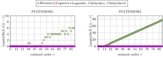
Under this condition we compare the numerical ranks of the associated observability matrices for certain orthogonal polynomials. Here, the tolerance of MATLAB^®s rank function was set to $10^{-20}$ to ensure a good rank estimation. The differences between the reduced orders $r$ and the numerical rank of the observability matrix are depicted in Figure 1. For the matrix pair $(S,L)$ we only consider an odd order $r$, for $(\hat{S},\hat{L})$ only an even order $r$ due to the invertibility conditions for the matrices $\tilde{E}$ and $\hat{E}$. There are two exceptions: Since the $\tilde{E}$ and $\hat{E}$ matrices are always invertible in case of Laguerre polynomials, their numerical rank is plotted for all $r$. Even though the $\hat{E}$ matrix using the Hermite polynomials is not invertible at all, we use here matrix pair $(\tilde{S},\tilde{L})$ from equation (17) and thus observability matrix (18) instead to obtain its numerical rank.

In both subfigures it is easy to see, that the Legendre and both types of Chebychev polynomials always lead to a full numerical rank. In case of these polynomials, the rank is only plotted with one mark, because the result is always the same. The Laguerre polynomials show the same behavior in both figures for all $r$. In contrast, the Hermite polynomials in SYLTDMOR2 only have a full numerical rank if the reduced order $r$ is small enough, i.e. $r\leq 14$. For SYLTDMOR1, their numerical rank is full only if $r\leq 27$.

Note, that Figure 1 only presents numerical ranks. We now, considering only our proposed new variant SYLTDMOR2, prove the full rank of the observability matrices for the Jacobi, Laguerre, Legendre and Chebychev polynomials of first and second kind rigorously. We will also show, that for the Hermite polynomials, theoretically, the rank of $Ob(\tilde{S},\tilde{L})$ is always full as opposed to the numerical rank.

To overcome the difficulties with the singularity of $\hat{E}$ for some kinds of orthogonal polynomials, we will rewrite Sylvester equation (12) as

$$A\hat{V}\hat{E}+E\hat{V}=B\begin{bmatrix}w_{1}&\ldots&w_{r}\end{bmatrix}\quad\Leftrightarrow\quad E\hat{V}-A\hat{V}\tilde{S}=B\tilde{L},$$ (17)

where $\tilde{S}=-\hat{E}$ and $\tilde{L}=\begin{bmatrix}w_{1}&\ldots&w_{r}\end{bmatrix}$, i.e. with the roles of $E$ and $A$ swapped.

Let $s_{1},\ldots,s_{r}\in\mathbb{C}\backslash\Lambda\left(E^{-1}A\right)$ be distinct expansion points, then

$$\text{span}\big{\{} (A-s_{1}E)^{-1}B,\ldots,(A-s_{r}E)^{-1}B\big{\}}$$

$$=\text{span}\Bigg{\{}-\frac{1}{s_{1}}\left(E-\frac{1}{s_{1}}A\right)^{-1}B,\ldots,-\frac{1}{s_{r}}\left(E-\frac{1}{s_{r}}A\right)^{-1}B\Bigg{\}}$$

$$=\text{span}\Bigg{\{}\left(E-\frac{1}{s_{1}}A\right)^{-1}B,\ldots,\left(E-\frac{1}{s_{r}}A\right)^{-1}B\Bigg{\}}.$$

Thus, the solution of the Sylvester equation (17) is a basis of a Krylov subspace with expansion points $\displaystyle\frac{1}{s_{i}}$ for $i=1,\ldots,r$.

4.3.1 Hermite Polynomials

Since for these polynomials the $\hat{E}$ matrix is singular for all $r$, we choose Sylvester equation (17) to prove the equivalence to moment matching. As mentioned above, we assume the input to be chosen piecewise constant and thus $\tilde{L}=\begin{bmatrix}1&0&\ldots&0\end{bmatrix}$. Further,

$$\tilde{S}=-\frac{1}{2}\begin{bmatrix}0&\displaystyle\frac{1}{2}&&\\ &\ddots&\ddots&\\ &&\ddots&\displaystyle\frac{1}{r}\\ &&&0\end{bmatrix}.$$

Due to this special structure, the $(r\times r)$ observability matrix is a diagonal matrix with non-zero entries

$$\text{diag}(Ob(\tilde{S},\tilde{L}))=\begin{bmatrix}1&\displaystyle-\frac{1}{2}\cdot\frac{1}{2}&\displaystyle\frac{1}{2^{2}}\cdot\frac{1}{2\cdot 3}&\ldots&\displaystyle\left(-\frac{1}{2}\right)^{r-1}\left(\prod\limits_{i=1}^{r-1}(i+1)\right)^{-1}\end{bmatrix}$$ (18)

and thus $(\tilde{S},\tilde{L})$ is observable. Converting this problem back to Sylvester equation (16), the expansion points are generalized eigenvalues of $(-\hat{E},I_{r})$ and thus inverse eigenvalues of $(-I_{r},\hat{E})$, where $\hat{E}=-\tilde{S}$. Since $\hat{E}$ is a strict upper triangular matrix, all eigenvalues of $(-I_{r},\hat{E})$ are zero and thus all expansion points are $\infty$ (see, e.g. [15], [16, Chapter 4]).

4.3.2 Laguerre Polynomials

Since the $\hat{E}$ matrix for these polynomials is always invertible, we choose Sylvester equation (12). The explicit inverse to

$$\hat{E}=\begin{bmatrix}-1&1&&\\ &\ddots&\ddots&\\ &&\ddots&1\\ &&&-1\\ \end{bmatrix}$$

is given by the upper triangular matrix

$$\hat{E}^{-1}=-\begin{bmatrix}1&\cdots&1\\ &\ddots&\vdots\\ &&1\end{bmatrix}.$$

Since $\hat{S}=-\hat{E}^{-1}$ by definition and due to the choice of piecewise constant inputs, we have

$$\hat{L} =\begin{bmatrix}1&0&\ldots&0\end{bmatrix}\hat{E}^{-1}=-\begin{bmatrix}1&\ldots&1\end{bmatrix}=-\hat{S}(1,:).$$

Thus the entries of the observability matrix become

$$Ob(\hat{S},\hat{L})=\begin{bmatrix}\hat{L}\\ \hat{L}\hat{S}\\ \vdots\\ \hat{L}\hat{S}^{r-1}\end{bmatrix}=-\begin{bmatrix}\hat{S}(1,:)\\ \hat{S}(1,:)\hat{S}\\ \vdots\\ \hat{S}(1,:)\hat{S}^{r-1}\end{bmatrix}=-\begin{bmatrix}\hat{S}(1,:)\\ \hat{S}^{2}(1,:)\\ \vdots\\ \hat{S}^{r}(1,:)\end{bmatrix}.$$

Observing that the first rows in the powers of $\hat{S}$ can be written in terms of binomial coefficients and using the sum formula

$$\sum_{k=0}^{n}\binom{k}{l}=\binom{n+1}{l+1},$$

for integers $k,l,n\geq 0$ (see, e.g. [17, Chapter 1]), and the properties

$$\binom{n}{0}=\binom{n}{n}=1,\quad\binom{n}{1}=\binom{n}{n-1}=n,\quad\binom{n}{k}=\binom{n-1}{k-1}+\binom{n-1}{k},$$

for integers $n,k\geq 1$, we obtain a structured observability matrix

$$Ob(\hat{S},\hat{L}) =-\begin{bmatrix}\binom{0}{0}&\binom{1}{0}&\binom{2}{0}&\cdots&\binom{r-1}{0}\\[3.00003pt] \binom{1}{0}&\binom{2}{1}&\binom{3}{2}&\cdots&\binom{r}{r-1}\\[3.00003pt] \binom{2}{0}&\binom{3}{1}&\binom{4}{2}&\cdots&\binom{r+1}{r-1}\\[3.00003pt] \vdots&\vdots&\vdots&\ddots&\vdots\\[3.00003pt] \binom{r-1}{0}&\binom{r}{1}&\binom{r+1}{2}&\cdots&\binom{2r-2}{r-1}\end{bmatrix}$$

$$=-\begin{bmatrix}1&1&1&\cdots&1\\ 1&2&3&\cdots&r\\ 1&3&6&\cdots&\frac{r(r+1)}{2}\\ \vdots&\vdots&\vdots&\ddots&\vdots\\ 1&r&\frac{r(r+1)}{2}&\cdots&\binom{2r-2}{r-1}\end{bmatrix},$$

that is known as the Pascal matrix. It can be shown (see, e.g. [18]), that the LU decomposition of this matrix leads to its triangular factors being triangular Pascal matrices, and thus the determinant is always 1. Consequently, $Ob(\hat{S},\hat{L})$ always has full rank and we have established the equivalence to moment matching choosing the expansion points as eigenvalues of $\hat{S}$, i.e. $s_{0}=1$.

4.3.3 Jacobi Polynomials (Including Legendre and Chebychev polynomials)

In this case we choose Sylvester equation (17) to avoid problems with a singular $\hat{E}$. As for the Hermite polynomials we consider $\tilde{L}~{}=~{}\begin{bmatrix}1&0&\ldots&0\end{bmatrix}.$

For this class of orthogonal polynomials, the $\tilde{S}$ matrix has the same structure and only differs in its entries $\alpha_{i},\beta_{i}$ and $\gamma_{i}$ for $i=1,\ldots,r$:

$$\tilde{S}=\begin{bmatrix}\beta_{1}&\alpha_{1}&&&\\ \gamma_{2}&\beta_{2}&\alpha_{2}&&\\ &\ddots&\ddots&\ddots&\\ &&\gamma_{r-1}&\beta_{r-1}&\alpha_{r-1}\\ &&&\gamma_{r}&\beta_{r}\\ \end{bmatrix}.$$

We now prove the full rank of the observability matrix by induction.

Base clause: If we compute the observability matrix for certain small $r$ with the above mentioned $\tilde{L}$ and $\tilde{S}$, we can clearly see a structure, namely:

$r$	$Ob(\tilde{S},\tilde{L})$	rank
$1$	$\begin{bmatrix}1\end{bmatrix}$	$1$
$2$	$\begin{bmatrix}1&0\\ \beta_{1}&\alpha_{1}\end{bmatrix}$	$2$
$3$	$\begin{bmatrix}1&0&0\\ \beta_{1}&\alpha_{1}&0\\ \beta_{1}^{2}+\alpha_{1}\gamma_{2}&\alpha_{1}\left(\beta_{1}+\beta_{2}\right)&\alpha_{1}\alpha_{2}\end{bmatrix}$	$3$

These matrices are lower triangular and obviously have full rank, since $\alpha_{i}\neq 0$ by definition.

Induction hypothesis: Now assume that the observability matrix of size $r\times r$ has a lower triangular structure

$$Ob(\tilde{S},\tilde{L})=\begin{bmatrix}1&&&\\ *&\alpha_{1}&&\\ \vdots&\ddots&\ddots&\\ *&\cdots&*&\prod\limits_{i=1}^{r-1}\alpha_{i}\end{bmatrix}$$

and full rank with $*$ representing the non-zero entries.

Induction step: To prove the lower triangular structure and the full rank of the observability matrix of size $(r~{}+~{}1)\times(r~{}+~{}1)$, we only need to have a closer look at the $r+1$st row and column since the $r\times r$ block is unchanged. Since the first row is the first unit vector by definition and $\tilde{S}$ is a tridiagonal matrix, the first $r$ entries of the last columns are equal to zero. The last row is computed by multiplying the $r$th row with $\tilde{S}$. Due to the tridiagonal structure the first $r$ entries are non-zero if $\alpha_{i},\beta_{i}$ and $\gamma_{i}$ are non-zero for $i=1,\ldots,r$. The $r+1$st entry is obtained by multiplying

$$\begin{bmatrix}*&\cdots&*&\prod\limits_{i=1}^{r-1}\alpha_{i}&0\end{bmatrix}\cdot\begin{bmatrix}0\\ \vdots\\ 0\\ \alpha_{r}\\ \beta_{r+1}\end{bmatrix}=\prod\limits_{i=1}^{r}\alpha_{i}.$$

Thus, the observability matrix is a lower triangular matrix whose diagonal entries are non-zero since $\alpha_{i}\neq 0\ \forall i$, which proves its full rank and completes the induction.

The proof for Legendre and Chebychev polynomials is omitted since these polynomials are special cases of the Jacobi polynomials (see, e.g. [5, Chapter 22]).

Figure 2: Minimal distance of generalized eigenvalues $(-\tilde{A},\tilde{E})$ and $(-I_{r},\hat{E})$

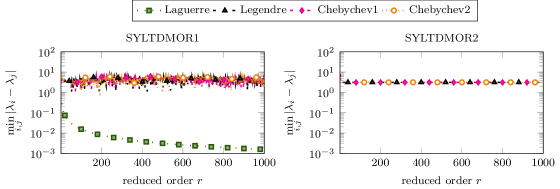
For SYLTDMOR2 presented in Section 3.2 we can apply Theorem 4.1 directly for the Hermite and Laguerre polynomials for SYLTDMOR2, since all generalized eigenvalues of $(-I_{r},\hat{E})$ are $\infty$ and $1$ respectively, and obtain an equivalence. Regarding the Legendre, Chebychev polynomials of first and second kind, the Jacobi polynomials in both approaches and the Laguerre polynomials for the original approach proposed in [1], we first have to prove the distinct eigenvalues before applying Theorem 4.2. Since this is hard to verify, we show in Figure 2 in the left subfigure the minimal distance between the generalized eigenvalues of $(-\tilde{A},\tilde{E})$ with matrices arising in Sylvester equation (11) in SYLTDMOR1 and in the right subfigure for the matrix pencil $(-I_{r},\hat{E})$, where $\hat{E}$ occurs in Sylvester equation (12) in the SYLTDMOR2 algorithm, for a reduced order $r=1,\ldots,1000$. A reduced order $r~{}>~{}1000$ is not desirable, since reducing the original system and simulating the ROM is done with dense matrices of dimension $r$ and thus the computational costs become $O(r^{2})$ or even $O(r^{3})$, when using an implicit solving scheme, which is way too expensive. Since, in the right subfigure, the minimal distance between the eigenvalues up to a reduced order of $r=1000$ is clearly larger than zero, even in finite precision, we conclude that one can apply Theorem 4.2 for the practically relevant $r$. Considering the Jacobi polynomials, we assume that $a,b>-1$ are chosen such that all eigenvalues are distinct.

Summarizing these findings, we have proven the equivalence to a Krylov subspace MOR method for SYLTDMOR2 presented in Section 3.2.

Theorem 4.4 (Equivalence between SYLTDMOR2 and moment matching).

Consider (1) with piecewise constant input.

If we choose

• Hermite polynomials,

• Laguerre polynomials,

• Legendre polynomials,

• Chebychev polynomials of first kind,

• Chebychev polynomials of second kind,

• Jacobi polynomials, choosing $a$ and $b$ such that all eigenvalues of $(-I_{r},\hat{E})$ are distinct,

then SYLTDMOR2 presented in Section 3.2 is equivalent to the moment matching method, where the expansion points are chosen to be the eigenvalues of the matrix pencil $(-I_{r},\hat{E})$ arising in Sylvester equation (12) and depend on the choice of the orthogonal polynomials and the reduced order.

Nevertheless, we have also shown the observability numerically in the left subfigure of Figure 1 for the Laguerre, Legendre and Chebychev polynomials of first and second kind. In the left subfigure of Figure 2 we can also see, that the minimal distance between the generalized eigenvalues of $(-\tilde{A},\tilde{E})$ is clearly larger than zero in case of Legendre and Chebychev polynomials of first and second kind. Hence, for these polynomials the eigenvalues are distinct. In case of the Laguerre polynomials the minimal distance seems to decrease, but for a reduced order of $r=1000$ the minimal distance is approximately $10^{-3}$. It is thus too large for a computational error from round off accumulation. Hence, also the generalized eigenvalues for the Laguerre polynomials are distinct for all relevant reduced orders $r$. Thus, we conjecture the equivalence to moment matching for the TDMOR approach of Jiang and Chen [1] and thus SYLTDMOR1:

Conjecture 4.5 (Equivalence between SYLTDMOR1 and moment matching).

Consider (1) with piecewise constant input and zero initial state.

If we choose

• Laguerre polynomials,

• Legendre polynomials, odd reduced order,

• Chebychev polynomials of first kind, odd reduced order,

• Chebychev polynomials of second kind, odd reduced order,

then SYLTDMOR1 presented in Section 3.1 is equivalent to the moment matching method, where the expansion points are chosen to be the eigenvalues of the matrix pencil $(-\tilde{A},\tilde{E})$ arising in Sylvester equation (11) and depend on the choice of the orthogonal polynomials and the reduced order.

Remark 4.6.

The equivalence between the Laguerre based time domain MOR and moment matching has been proven rigorously by Eid in [12].

4.4 Advantages of Moment Matching over SYLTDMOR(1/2) in Practice

Comparing the polynomial based time domain MOR with moment matching one should keep in mind, that the expansion points can be freely chosen using moment matching. Since we use an IRKA based algorithm to determine the rational Krylov subspace, these expansion points will be optimized fitting to the original LTI system. Computing the reduced system with the time domain framework of Jiang and Chen presented in Section 2 or SYLTDMOR2 in Section 3.2, the expansion points are fixed by the choice of the family of polynomials. Exemplary, these expansion points or equivalently the generalized eigenvalues of matrix pairs $(-\tilde{A},\tilde{E})$ (SYLTDMOR1) and $(-I_{r},\hat{E})$ (SYLTDMOR2), are shown in Figure 3 for a reduced order $r=40$.

Figure 3: Generalized eigenvalues of $(-\tilde{A},\tilde{E})$ and $(-I_{r},\hat{E})$ for $r=40$

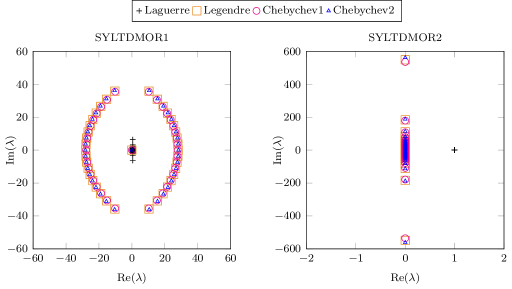
Thus, a variation of the expansion points arising from the time domain approach can be achieved by in- or decreasing the reduced order $r$ or rather using another family of orthogonal polynomials, on the one hand. On the other hand, orthogonal polynomials of higher degree $s\in\mathbb{Z}$ up to degree $s+r-1$ could be used or $r$ arbitrarily chosen orthogonal polynomials. To the best of our knowledge this has not been tried in the open literature so far.

Considering the choice of expansion points, the time domain MOR framework based on orthogonal polynomials, thus only seems to be a restriction of moment matching to a rather limited set of possible combinations. Thus, in practice IRKA has to be expected to provide more accurate ROMs in almost all cases. Further, IRKA has to be at least as good as the discussed time domain MOR approaches.

5 Numerical Examples

To illustrate the effectiveness of the time domain MOR techniques based on orthogonal polynomials, but also to confirm our conjecture about the restriction of this method compared to moment matching, we will present results for three well-known test examples.

The basic setup for the first two examples is the same, namely:

• initial state $x_{0}=\mathbb{O}_{n,1}\in\mathbb{R}^{n},$

• time interval $t\in[0,1]$, i.e. $t_{0}=0$,

• time step $\tau=0.001$,

• input $u(t)=\begin{cases}0\qquad&,t\in[0,0.1)\\ \frac{1}{2}\sin\left(\pi(10t-\frac{3}{2})\right)+\frac{1}{2}\quad&,t\in[0.1,0.2)\\ 1&,t\in[0.2,1]\end{cases}.$

The test system is always the following:

• CPU: 2x Intel^® Xeon^® X5650

  • $6$ Cores per CPU,

  • clock rate: $2.67$ GHz,

  • $12$ MB Cache per CPU,

• memory: $48$ GB DDR3 with ECC.

All examples are computed using MATLAB^® R2012b.

In this paper, we illustrate the 2-norm averaged relative error over time, i.e.

$$\left\|\frac{y(t)-y_{r}(t)}{y(t)}\right\|_{2,[0,1]} =\left(\int\limits_{0}^{1}\left(\frac{y(t)-y_{r}(t)}{y(t)}\right)^{2}dt\right)^{\frac{1}{2}}$$

$$\approx\left(\sum\limits_{i=1}^{\frac{1}{\tau}}\left(\frac{y(i\tau)-y_{r}(i\tau)}{y(i\tau)}\right)^{2}\right)^{\frac{1}{2}},$$

where $y(t)$ and $y_{r}(t)$ are computed using the implicit Euler method (see, e.g. [19, Chapter 2]). Note, that the $\infty$-norm averaged error over time looks comparable and is thus not illustrated. We also show the total time, that was spent to reduce the original LTI system and to solve the reduced LTI system compared to the time, that was spent on solving the original LTI system. In these figures, we compare SYLTDMOR1 and SYLTDMOR2 to the two most important and well accepted methods for stable LTI systems, IRKA (one- and two-sided) and balanced truncation. For the one-sided IRKA approach, the projection matrix $V$ is computed from the output Krylov subspace, i.e. in case of one expansion point $s_{0}$ $V$ is the basis of $\mathcal{K}_{r}\left((A-s_{0}E)^{-T}E^{T},(A-s_{0}E)^{-T}C^{T}\right)$. In case of multiple expansion points $s_{1},\ldots,s_{r}$ $V$ is a basis of $\bigcup\limits_{i=1}^{r}\mathcal{K}_{r_{i}}\left((A-s_{i}E)^{-T}E^{T},(A-s_{i}E)^{-T}C^{T}\right)$. This is implemented according to the theory in Section 4 and does not present a restriction to moment matching since upon convergence of IRKA, the expansion points are (locally) optimally placed for the system with respect to $\mathcal{H}_{2}$ approximation. In the figures, we use the following notations for Chebychev polynomials of first (Chebychev1) and second kind (Chebychev2), the one-sided IRKA resp. moment matching (oIRKA/oMM), the two-sided IRKA resp. moment matching (IRKA/tMM) and balanced truncation (BT). Note, that we computed $50$ cycles to average the results.

5.1 Triple Peak Example

Our first example is the triple peak, sometimes also called FOM, example (see, e.g. [20]), where the dynamical system (1) of order $n=1\,006$ is given by

Figure 4: Relative errors (triple peak example of Section 5.1)

$E=I_{n},A\in\mathbb{R}^{1\,006\times 1\,006}$ a block diagonal matrix of the form

$$A =\begin{bmatrix}A_{1}&&&\\ &A_{2}&&\\ &&A_{3}&\\ &&&A_{4}\\ \end{bmatrix},\quad A_{1} =\begin{bmatrix}-1&100\\ -100&-1\end{bmatrix},$$

$$A_{2} =\begin{bmatrix}-1&200\\ -200&-1\end{bmatrix},\qquad\qquad\ A_{3} =\begin{bmatrix}-1&400\\ -400&-1\end{bmatrix},$$

$$A_{4} =\text{diag}\{-1,-2,\ldots,-1\,000\},$$

and the input and output matrices are

$$B^{T}=C=[\underbrace{10,\ldots,10}_{6},\underbrace{1,\ldots,1}_{1\,000}]\in\mathbb{R}^{1\times 1\,006}.$$

That means $x(t)\in\mathbb{R}^{1\,006}$ and $u(t),y(t)\in\mathbb{R}$.

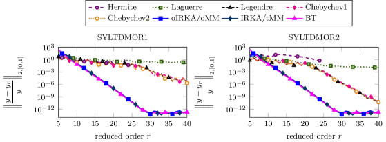
In Figure 4 the $2$-norm averaged relative error over time is illustrated for the reformulated time domain approach SYLTDMOR1, presented in Section 3.1, and its variation SYLTDMOR2, presented in Section 3.2, for Hermite, Laguerre, Legendre and Chebychev polynomials of first and second kind, each compared to the one- and two-sided IRKA and balanced truncation. In both subfigures we can easily see, that the frequency domain MOR approaches approximate the original system, for a reduced order $r\geq 11$, much better than the time domain approaches. Only the Legendre and the two Chebychev polynomial families in SYLTDMOR2 show a considerable decay of the relative error ending up with a relative error of $10^{-10}$ for a reduced order $r=40$. The same orthogonal polynomials in SYLTDMOR1 have only a slight decay of the relative error ending up at around $10^{-5}$ for a reduced order $r=40$. Compared to this, balanced truncation and both IRKA approaches show a nicer decay ending with a relative error of $10^{-12}$ for $r\geq 28$ and are thus at least $2$ orders lower compared to the Legendre and both Chebychev polynomials for both represented time domain approaches. Regarding the Laguerre polynomials the relative error does not seem to change for an increasing reduced order $r$ and stagnates around $10^{-1}$. This phenomenon can be explained, if we look at their differential recurrence coefficients stated in Table 2. These coefficients are constant and do not depend on the reduced order $r$ such that matrix $\hat{S}$ is always a triangular matrix with only $1$ on the diagonal as seen in Section 4.3.2. Thus the only expansion point of these polynomials for SYLTDMOR2, given by the multiple eigenvalue of $\hat{S}$, is $1$ with multiplicity $r$. That means in the sense of moment matching, that moments up to order $r$ are matched. But on the other hand all other important frequencies are ignored leading to a bad approximation. Considering SYLTDMOR1 it might be possible that this effect is also caused by the clustering of the eigenvalues. A special case are the Hermite polynomials, since they are only illustrated until $r=24$. The reason for this is the extreme condition number, i.e. numerical singularity, of the matrices $H$ and $\hat{H}$, which makes it impossible to solve the linear system of equations.

Figure 5: Condition numbers using Hermite polynomials

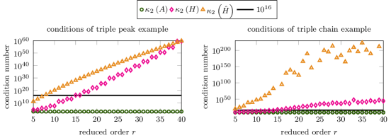
To get an impression how the condition numbers grow by increasing the reduced order, the $2$-norm condition numbers $\kappa_{2}(.)$ using Hermite polynomials are shown for the triple peak example presented in Section 5.1 and the example of the following Section 5.2 for the matrices $A,H$ and $\hat{H}$ in Figure 5. Since in MATLAB^® a matrix is numerically not invertible for $\kappa_{2}(.)>10^{16}$, this bound is added in the subfigures of Figure 5. Nevertheless, we can easily see in Figure 4, that the Hermite polynomials have a large relative error of around $10^{-1}$ in SYLTDMOR1 and about $10^{0}$ in SYLTDMOR2 at $r=24$, such that the original system is not approximated well.

The total time, that is spent on reducing the original system and solving the reduced system, is illustrated in Figure 6 and is compared to the time, that is needed to solve the original $(1\,006\times 1\,006)$ system. This figure is divided into three subfigures containing the reduction and solution times for determining $V$ by solving the huge $(nr\times nr)$ linear system of equations (9) with MATLAB^®’s backslash operator and Sylvester equations (11) and (12) with the method from [21]. In all three subfigures of Figure 6 it is easy to see, that all solution methods are faster than solving the original system. Comparing the time with the backslash operator and solving a Sylvester equation, irrespective whether SYLTDMOR1 or SYLTDMOR2 is chosen, the Sylvester solver is, for $r=40$, up to two times faster than solving with MATLAB^®’s backslash. For a reduced order of $r\geq 34$ there is an increase of the total time for both IRKA variants. The reason for this can be found in Figure 4, since the relative error of these methods is close to machine precision and thus an improvement of the relative error is not possible.

Figure 6: Total time (triple peak example of Section 5.1)

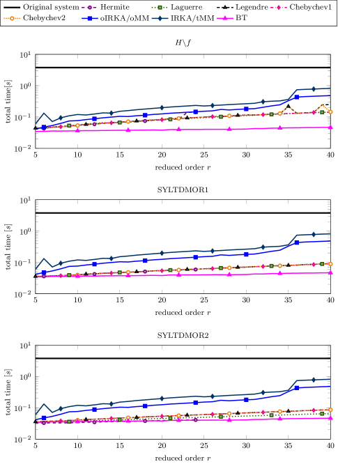
Basically, this example demonstrates, that the time domain MOR framework [1] reduces the LTI system fast. Further, these time domain MOR approach might be even faster by inserting the eigenvalues of matrix pencils $(-\tilde{A},\tilde{E})$ or $(-I_{r},\hat{E})$ directly as expansion points in the moment matching method ending up with the same projection matrix according to Theorem 4.4 and Conjecture 4.5. This could be implemented by precomputing the generalized eigenvalues and saving them in a data base, such that they are quickly available. Here, the Jacobi polynomials are excluded, since they require a further analysis of the choice of parameters $a$ and $b$. Nevertheless, this example also demonstrates, that the time domain MOR approaches are less accurate compared to IRKA or balanced truncation.

5.2 Triple Chain Example

The second example is the triple chain example from [22], i.e. three mass-spring-damper chains of length $200$ are fixed by one coupling mass. Since this example, which is parametrized as in [23], results in a second order systems

$$\begin{split}M\ddot{x}(t)+D\dot{x}(t)+Kx(t)&=\mathcal{B}u(t),\\ y(t)&=\mathcal{C}x(t),\end{split}$$ (19)

we transform it into the first order system

$$\underbrace{\begin{bmatrix}K&0\\ 0&M\end{bmatrix}}_{E}\underbrace{\begin{bmatrix}\dot{x}(t)\\ \ddot{x}(t)\end{bmatrix}}_{\dot{z}(t)} =\underbrace{\begin{bmatrix}0&K\\ -K&-D\end{bmatrix}}_{A}\underbrace{\begin{bmatrix}x(t)\\ \dot{x}(t)\end{bmatrix}}_{z(t)}+\underbrace{\begin{bmatrix}0\\ \mathcal{B}\end{bmatrix}}_{B}u(t),$$

$$y(t) =\underbrace{\begin{bmatrix}\mathcal{C}&0\end{bmatrix}}_{C}\underbrace{\begin{bmatrix}x(t)\\ \dot{x}(t)\end{bmatrix}}_{z(t)}.$$

Here, the matrices of the second order system (19) are given by a diagonal matrix $M\in\mathbb{R}^{601\times 601}$ containing the masses, the damper matrix $D\in\mathbb{R}^{601\times 601}$ and the stiffness matrix $K\in\mathbb{R}^{601\times 601}$. The input and output matrices are again transposes of each other given by $\mathcal{B}^{T}=\mathcal{C}=[1\ldots 1]\in\mathbb{R}^{1\times 601}$. Hence, $E,A\in\mathbb{R}^{1\,202\times 1\,202},B^{T},C\in\mathbb{R}^{1\times 1\,202},z(t)\in\mathbb{R}^{1\,202}$ and $u(t),y(t)\in\mathbb{R}$.

Figure 7: Relative errors (triple chain example of Section 5.2)

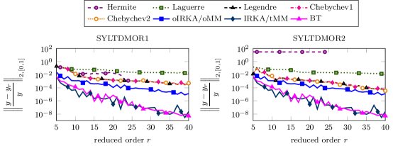
Figure 7 illustrates the $2$-norm averaged relative error over time for the time domain MOR approaches compared to the frequency domain MOR methods as mentioned in the previous example. Again, the relative error using Laguerre polynomials shows only minor changes and is for a reduced order $r=40$ at around $10^{-1}$ using SYLTDMOR1 or SYLTDMOR2. Similar to the Laguerre polynomials, the Hermite polynomials do not approximate the original system well since the relative error is, especially in case of SYLTDMOR2, too large, namely $29$ for a reduced order $r=24$. In case of SYLTDMOR1 the relative error decreases to around $10^{-2}$, but since the $H$ matrix is numerically singular, it is not possible to determine further projection matrices. In both subfigures the 2-norm averaged relative error over time decreases, if Legendre or Chebychev polynomials of first or second kind are used. This relative error is around $10^{-3}$ for SYLTDMOR1 and $10^{-4}$ for SYLTDMOR2, for a reduced order $r=40$. Comparing both time domain approaches to the one-sided IRKA algorithm, we can clearly see, that the relative error using moment matching is always at least as small as in case of the time domain MOR, but mostly even smaller. Looking at the two-sided IRKA algorithm and the balanced truncation method, we see, that these methods are even more successful since they have a steeper decrease of the relative error ending up with a relative error of order $10^{-8}$, which is $4$ orders of magnitude lower than for the one-sided method.

Figure 8: Total time (triple chain example of Section 5.2)

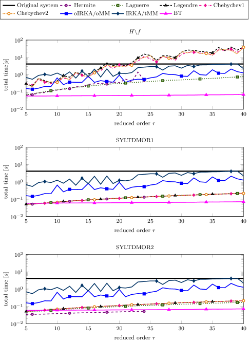
We now take look at the total time, i.e. the time needed to reduce the original system and to simulate the reduced system. In the upper subfigure of Figure 8, illustrating the total time for the backslash solver, we can easily see that, if we use the time domain approach with Hermite and Laguerre polynomials, we are faster than solving the original system. Unfortunately, these polynomials do not approximate the original system well. Using the Legendre or one of the Chebychev families, this approach is faster than simulating the original system until $r=21$. Hence, considering a larger reduced order is not effective any more. If we use one of the Sylvester solvers instead, we can achieve a high speed-up, e.g. choosing a reduced order $r=40$, we can reduce the system and simulate the reduced system up to $19$ times faster than simulating the original system. This also holds for the Hermite and Laguerre polynomials. The former ones are only considered up to a reduced order $r=24$. Regarding both IRKA implementations and balanced truncation, it is clearly visible, that these MOR techniques consume more time than the time domain approaches using Sylvester equations. Nevertheless, these methods are still faster than simulating the original triple chain example.

5.3 Butterfly Gyroscope Example

A more practice oriented and larger example is given by the butterfly gyroscope example from the Oberwolfach benchmark collection for model order reduction (see, [24]) described in [25], which represents a vibrating micro-mechanical gyroscope. The device consists of a three-layer silicon wafer stack. Its middle layer contains the sensor element, which consists of two wing pairs that are connected to a common frame – the reason the gyro is called butterfly. This example is given as second order system (19) and transformed into a first order realization

$$\underbrace{\begin{bmatrix}-K^{T}&0\\ 0&M\end{bmatrix}}_{E}\underbrace{\begin{bmatrix}\dot{x}(t)\\ \ddot{x}(t)\end{bmatrix}}_{\dot{z}(t)} =\underbrace{\begin{bmatrix}0&-K^{T}\\ -K&-D\end{bmatrix}}_{A}\underbrace{\begin{bmatrix}x(t)\\ \dot{x}(t)\end{bmatrix}}_{z(t)}+\underbrace{\begin{bmatrix}0\\ \mathcal{B}\end{bmatrix}}_{B}u(t)$$

$$y(t) =\underbrace{\begin{bmatrix}\mathcal{C}&0\end{bmatrix}}_{C}\underbrace{\begin{bmatrix}x(t)\\ \dot{x}(t)\end{bmatrix}}_{z(t)}.$$

Here, matrices $M,D,K\in\mathbb{R}^{17\,361\times 17\,361}$ of the second order system are symmetric matrices, the input is the vector $\mathcal{B}\in\mathbb{R}^{17\,361}$ and output matrix is given as $\mathcal{C}\in\mathbb{R}^{12\times 17\,361}$. In order to obtain a SISO system, we only consider the first row of $\mathcal{C}$. Hence the matrices and vectors of the first order system are of dimension $E,A\in\mathbb{R}^{34\,722\times 34\,722},B^{T},C\in\mathbb{R}^{1\times 34\,722},z(t)\in\mathbb{R}^{34\,722}$ and $u(t),y(t)\in\mathbb{R}$.

Accounting for the output trajectory, we changed the computational setup for this example to

• time interval $t\in[0,0.005]$,

• time step $\tau=5\cdot 10^{-6}$, and

• input $u(t)$ the corresponding sine-smoothed step from 0 to 1 in the interval $[0.0005,0.001]$.

However, this can easily be transformed to a time interval $t\in[0,1]$ using the transformation $t_{1}=\frac{t_{1}}{0.005}$ with time step $\tau=0.001$ as in the previous examples. The initial state $x_{0}$ and the input $u(t)$ are chosen as in the previous examples. Furthermore, we computed only one cycle instead of $50$ to limit the computation time, since external effects are expected to be far less influential in this case.

Figure 9: Relative errors (butterfly gyroscope example of Section 5.3)

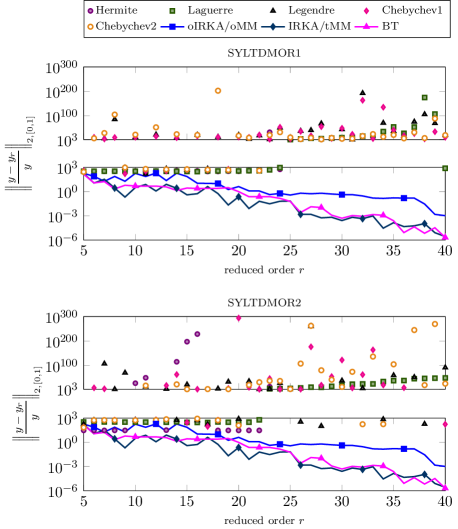
In Figure 9 the $2$-norm averaged relative error over time is illustrated. These subfigures differ from the ones from the previous examples. Here, each subfigure consists of two plots, where the upper plot is logarithmically scaled from $10^{3}$ to $10^{300}$ and the lower plot is logarithmically scaled from $10^{-6}$ to $10^{3}$. The reason for this unusual scaling are large differences of the relative errors of the time domain MOR approach using orthogonal polynomials compared to the remaining MOR methods as IRKA and balanced truncation. While the maximum relative error of the remaining methods is around $10^{3}$, the minimum relative error of the orthogonal polynomials is in the same area and increases even up to an order of $10^{294}$. Furthermore it is even possible, that this method produces unsuitable, i.e. non stable ROMs. Then the relative error is given by NaN and omitted in the plot. Compared to this, the relative error for the balanced truncation method and both IRKA approaches nicely decreases. Looking at reduced order $r=40$, balanced truncation and the two-sided IRKA method end up with a relative error of around $10^{-5}$ and the one-sided IRKA approach with a relative error of around $10^{-2}$. Thus Figure 9 illustrates impressively, that the orthogonal polynomial based time domain MOR framework fails completely for this example.

Figure 10: Total time (butterfly gyroscope example of Section 5.3)

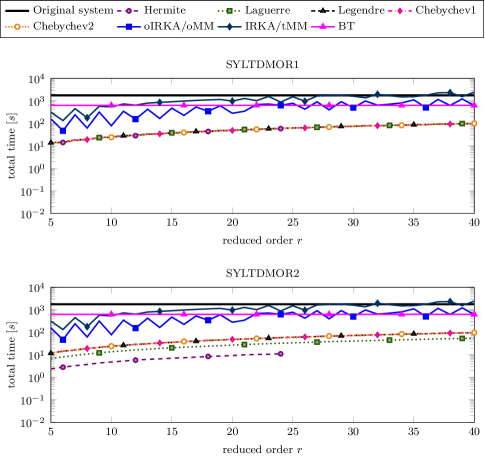
Figure 10 illustrates the total time that is needed to reduce and simulate the reduced system. Just like in the previous examples, SYLTDMOR1 and SYLTDMOR2 are clearly faster than using one of the IRKA approaches or the balanced truncation method. Still, the increased computation time is a price worth paying, since the latter methods produce suitable and reliable ROMs in all test cases. Note, that we cannot report the total time using MATLAB^®’s backslash operator, since the computations became too memory consuming even for our well equipped test system.

If we now take the relative errors illustrated in Figure 9 into account, IRKA and balanced truncation are clearly more desirable than the time domain MOR techniques, since all of them approximate the original model behavior far better.

Figure 11: Smoothed step-response trajectories of the three test examples.

5.4 Observations

The numerical examples, reported above, give us an impression of the effectiveness of the time domain framework of Jiang and Chen and its variation SYLTDMOR2 compared to other frequency domain MOR techniques. Regarding the relative errors, the one- and two-sided IRKA algorithm and balanced truncation always have a stronger decrease and thus (almost) always smaller relative errors. The fact, that these methods consume more time than the time domain approaches is negligible, since these methods (nearly) always performed faster than solving the original system.

Note, that we also tried to implement the iterative splitting method proposed in [1], but our implementation never converged for the above mentioned examples. Thus, we are not able to compare with our proposed solving techniques. Since solving with MATLAB^®s backslash operator is time-consuming, we also tried to solve (9) using the preconditioned Generalized Minimum Residual (GMRES) method. But since the matrix $H$ in (9) is ill-conditioned, we were not able to find a good preconditioner, such that (9) can be solved fast.

The aim of model reduction in our context is to find a reduced system approximating the original system well, such that the time, that is spent on reducing and solving the reduced system, is less than simulating the original system. SYLTDMOR1 and its variation SYLTDMOR2 clearly consume less time than solving the original system, but the relative error either decreases very slowly as in the first two examples and thus the reduced order needs to be comparably large or the computed ROM is not suitable at all. This behavior can be easily explained when looking at the trajectories of all examples illustrated in Figure 11. The trajectories of the triple peak and the triple chain example can easily be expressed by using low-order polynomials. In contrast to this, the trajectory of the butterfly gyroscope example is oscillating rather fast and thus it requires higher order polynomial to approximate the solution properly, which are not present in the bases generating low-order models following the Jiang/Chen framework.

6 Concluding Remarks

In this paper, we picked up the time domain MOR framework based on the idea of Jiang and Chen in [1] and transformed the resulting huge linear system of equations into a Sylvester equation, that can be solved very efficiently. A slight variation of the formulation leads to another even nicer Sylvester equation considering a fixed initial state and leading to easier structure in the small coefficient matrices. Using the duality theorem, we show a connection of the time domain MOR methods to moment matching, but we also illustrate, that the expansion points created by the time domain approaches cannot adapt to the system and thus the time domain approaches in this paper cannot keep up with proper moment matching, which is only one iteration step of IRKA.

Code Availability

The MATLAB^® implementation used to compute the presented results can be obtained from

doi: 10.5281/zenodo.1243090

and is authored by: Manuela Hund and Jens Saak.

References

- [1] Y.L. Jiang and H.B. Chen, Time domain model order reduction of general orthogonal polynomials for linear input-output systems, IEEE Trans. Autom. Control 57 (2012), pp. 330–343.
- [2] S. Gugercin, A.C. Antoulas, and C.A. Beattie, model reduction for large-scale linear dynamical systems, SIAM J. Matrix Anal. Appl. 30 (2008), pp. 609–638.
- [3] Y. Xu and T. Zeng, Optimal model reduction for large scale MIMO systems via tangential interpolation, Int. J. Numer. Anal. Model. 8 (2011), pp. 174–188.
- [4] A.C. Antoulas, Approximation of Large-Scale Dynamical Systems, Adv. Des. Control Vol. 6, SIAM Publications, Philadelphia, PA, 2005.
- [5] M. Abramovitz and I.A. Stegun (eds.), Pocketbook of mathematical functions, Verlag Harry Deutsch, 1984, abridged edition of ”Handbook of mathematical functions” (1964).
- [6] K.B. Datta and B.M. Mohan, Orthogonal functions in systems and control, Advanced Series in Electrical and Computer Engineering Vol. 9, World Scientific Publishing Co., Inc., River Edge, NJ, 1995.
- [7] R.A. Horn and C.R. Johnson, Topics in Matrix Analysis, Cambridge University Press, Cambridge, 1991.
- [8] M. Heinkenschloss, T. Reis, and A.C. Antoulas, Balanced truncation model reduction for systems with inhomogeneous initial conditions, Automatica 47 (2011), pp. 559–564.
- [9] C. Beattie, S. Gugercin, and V. Mehrmann, Model reduction for systems with inhomogeneous initial conditions, Syst. Control Lett. 99 (2017), pp. 99–106.
- [10] T. Wolf, pseudo-optimal model order reduction, Dissertation, Technische Universität München, Munich, Germany, 2015.
- [11] K. Yosida, Functional analysis, Classics in Mathematics, Springer-Verlag, Berlin, Heidelberg, 1995, reprint of the sixth (1980) edition.
- [12] R. Eid, Time domain model reduction by moment matching, Dissertation, Technische Universität München, Munich, Germany, 2009.
- [13] A. Vandendorpe, Model reduction of linear systems, an interpolation point of view, Ph.D. diss., Université Catholique De Louvain, Lleuven, Belgium, 2004.
- [14] M. Hund, Zeitbereichs-Modellreduktion und Sylvester-Gleichungen, Master’s thesis, Otto-von-Guericke-Universität, Magdeburg, Germany, 2015, Available at http://nbn-resolving.de/urn:nbn:de:gbv:ma9:1-7794.
- [15] E.J. Grimme, Krylov projection methods for model reduction, Ph.D. Thesis, Univ. of Illinois at Urbana-Champaign, USA, 1997.
- [16] J.W. Demmel, Applied numerical linear algebra, Society for Industrial and Applied Mathematics (SIAM), Philadelphia, PA, 1997.
- [17] D.E. Knuth, The art of computer programming. Vol. 1: Fundamental algorithms, Second printing, Addison-Wesley Publishing Co., Reading, Mass.-London-Don Mills, Ont, 1969.
- [18] R. Brawer and M. Pirovino, The linear algebra of the Pascal matrix, Linear Algebra Appl. 174 (1992), pp. 13–23.
- [19] J.C. Butcher, Numerical methods for ordinary differential equations, John Wiley & Sons, Ltd, Chichester, 2003.
- [20] T. Penzl, Algorithms for model reduction of large dynamical systems, Technical report SFB393/99-40, Sonderforschungsbereich 393 Numerische Simulation auf massiv parallelen Rechnern, TU Chemnitz, 09107 Chemnitz, FRG, 1999, Available at http://www.tu-chemnitz.de/sfb393/sfb99pr.html.
- [21] P. Benner, M. Köhler, and J. Saak, Sparse-dense Sylvester equations in -model order reduction, Preprint MPIMD/11-11, Max Planck Institute Magdeburg, 2011.
- [22] N. Truhar and K. Veselić, An efficient method for estimating the optimal dampers’ viscosity for linear vibrating systems using Lyapunov equation 31 (2009), pp. 18–39.
- [23] J. Saak, Efficient numerical solution of large scale algebraic matrix equations in PDE control and model order reduction, Dissertation, Technische Universität Chemnitz, Chemnitz, Germany, 2009, Available at http://nbn-resolving.de/urn:nbn:de:bsz:ch1-200901642.
- [24] Oberwolfach Benchmark Collection, Butterfly Gyroscope, hosted at MORwiki – Model Order Reduction Wiki (2004). Available at http://modelreduction.org/index.php/Butterfly_Gyroscope.
- [25] D. Billger, The Butterfly Gyro, in Dimension Reduction of Large-Scale Systems, Lect. Notes Comput. Sci. Eng. Vol. 45. Springer-Verlag, Berlin/Heidelberg, Germany, 2005, pp. 349–352.