Uniform asymptotic stability
of a fractional tuberculosis model

Abstract

We propose a Caputo type fractional-order mathematical model for the transmission dynamics of tuberculosis (TB). Uniform asymptotic stability of the unique endemic equilibrium of the fractional-order TB model is proved, for any $\alpha\in(0,1)$. Numerical simulations for the stability of the endemic equilibrium are provided.

1. Introduction

When defining a differential operator, one often employs, besides ordinary derivatives, generalized derivatives, which appear in a natural way when considering extensions of differential operators defined on differentiable functions, and weak derivatives, related to the transition to the adjoint operator MyID:298 . Derivatives of fractional and negative orders appear when the differentiation is defined by means of an integral transform, applicable to the domain of definition and range of such generalized differential operator MyID:310 . This is often done in order to obtain the simplest possible representation of the corresponding differential operator of a function and to attain a reasonable generality in the formulation of problems and satisfactory properties of the objects considered book:frac . Problems in the theory of differential equations, e.g., problems of existence, uniqueness, regularity, continuous dependence of the solutions on the initial data or on the right-hand side, or the explicit form of a solution of a differential equation defined by a given differential expression, are readily interpreted in the theory of operators as problems on the corresponding differential operator defined on suitable function spaces MR3200762 . One advantage of fractional order differential equations is that they provide a powerful instrument to incorporate memory and hereditary properties into the systems, as opposed to the integer order models, where such effects are neglected or difficult to incorporate GonzalezParra . Moreover, in order to precisely reproduce the nonlocal, frequency- and history-dependent properties of power law phenomena, some different modeling tools, based on fractional operators, have to be introduced: see, e.g., Atangana and references therein.

Communicable diseases have always been an important part of human history Brauer:17 . Fractional-order differential system models for infectious disease dynamics have been introduced in recent years AhmedPhysicaA2007 , DingYeFracHIVCD4cells , GonzalezParra , FracCarlaPintoMalaria , SofiaShakoorDelfim , ZhangDDNS2015 . In SofiaShakoorDelfim , the authors propose a fractional-order model and show, through numerical simulations, that the fractional models fit better the first dengue epidemic recorded in the Cape Verde islands off the coast of west Africa, in 2009, when compared with the standard differential model. The authors of GonzalezParra show that a nonlinear fractional order epidemic model is well suited to provide numerical results that agree very well with real data of influenza A (H1N1) at the population level. In FracCarlaPintoMalaria , a fractional model for malaria transmission is considered and numerical simulations are done for the variation of the values of the fractional derivative and of the parameter that models personal protection. In ZhangDDNS2015 , fractional-order derivatives are introduced into an HIV infection model and local asymptotic stability is proved. The authors of DingYeFracHIVCD4cells introduce fractional-order derivatives into a model of HIV infection of $CD4^{+}$ T-cells and analyze the local asymptotic stability of the equilibrium points. In VargasDeLeon201575 , the uniform asymptotic stability is proved extending the Volterra-type Lyapunov functions to fractional-order epidemic systems. Fractional-order predator-prey models are investigated in AhmedMMA2007 . In particular, existence and uniqueness of solutions are proved, and stability of equilibrium points studied. Numerical solutions of such models were obtained AhmedMMA2007 . Here we are interested to investigate fractional calculus with respect to tuberculosis.

Tuberculosis (TB) is a bacterial disease caused by Mycobacterium tuberculosis, which is usually spread through the air by people with active TB. TB is one of the top ten causes of death worldwide, which justifies the amount of research on the area: see, e.g., MyID:353 , MyID:271 , reportWHO2016 . For a good survey on optimal models of TB, we refer the reader to MyID:301 . In MyID:353 , delays are introduced in a TB model, representing the time delay on the diagnosis and commencement of treatment of individuals with active TB infection. Optimal control strategies to minimize the cost of interventions, considering reinfection and post-exposure interventions, are investigated in MyID:271 . In MyID:305 , the potential of two post-exposure interventions, treatment of early latent TB individuals and prophylactic treatment/vaccination of persistent latent TB individuals, is investigated. A mathematical model for TB is studied in MyID:314 from the optimal control point of view, using a multiobjective approach. For numerical simulations using TB data from Angola see MyID:230 . Despite the numerous works on tuberculosis, the literature on fractional-order mathematical models for TB is scarce. In Sweilama:2016 , the authors propose a multi-strain TB model of variable-order fractional derivatives and develop a numerical scheme to approximate the endemic solution numerically. Here, we propose a Caputo type fractional-order mathematical model for the transmission dynamics of tuberculosis (TB), based on the nonlinear differential system studied in Yang201079 , and investigate its stability.

The stability question is of main interest in epidemiological control systems Matignon1996 , MyID:355 , MyID:373 . For nonlinear fractional-order systems, stability analysis is a recent and interesting topic: see, e.g., Baleanu:2010 , Chen2014633 , Delavari2012 , LiChen:Automatica:2009 , LiChen:CMA:2010 , LiMa2013 , LiZhang:2011 , Rivero:2013 , VargasDeLeon201575 . The direct Lyapunov method provides a way to determine (asymptotic, uniform, global asymptotic) stability of an equilibrium point without explicitly solving for integer-order nonlinear systems VargasDeLeon201575 . In Delavari2012 , the authors extended the Lyapunov direct method to Caputo type fractional-order nonlinear systems using Bihari’s inequality and Bellman–Grownwall’s inequality. Different approaches for the extension of the Lyapunov direct method were proposed in Baleanu:2010 , LiChen:Automatica:2009 , LiChen:CMA:2010 . See LiZhang:2011 , Petras:2009 , Petras:2011 , Rivero:2013 , Trigeassou:2011 for a survey on stability analysis of fractional differential equations. In Sweilama:2016 , the stability of the endemic equilibrium of a fractional-order TB model is studied numerically. Here we prove, analytically, the uniform asymptotic stability of the unique endemic equilibrium of the fractional-order TB model, for any $\alpha\in(0,1)$. Moreover, we illustrate the theoretical stability results through numerical simulations.

The paper is organized as follows. In Section 2, we present basic definitions and some known results about Caputo fractional calculus as well as results on uniform asymptotic stability and Volterra-type Lyapunov functions for fractional-order systems. In Section 3, we introduce Caputo fractional-order derivatives into the TB model proposed in Yang201079 and study the existence of equilibrium points. In Section 4, we prove the uniform asymptotic stability of the unique endemic equilibrium of the fractional-order TB model. Numerical simulations are provided in Section 5, which illustrate the stability result proved in the previous section. We finish with Section 6 of conclusions.

2. Preliminaries on the Caputo fractional calculus

We begin by introducing the definition of Caputo fractional derivative and recalling its main properties.

[See GJI:GJI529 ] Let $a>0$, $t>a$, $\alpha,a,t\in\mathbb{R}$. The Caputo fractional derivative of order $\alpha$ of function $f\in C^{n}$ is given by

$$_{a}^{C}D_{t}^{\alpha}f(t)=\dfrac{1}{\Gamma(n-\alpha)}\int_{a}^{t}\dfrac{f^{(n)}(\xi)}{(t-\xi)^{\alpha+1-n}}d\xi,\qquad n-1<\alpha<n\in\mathbb{N}.$$ (2.1)

[Linearity, see, e.g., Diethelm ] Let $f(t),g(t):[a,b]\rightarrow\mathbb{R}$ be such that ${}_{a}^{C}D_{t}^{\alpha}f(t)$ and ${}_{a}^{C}D_{t}^{\alpha}g(t)$ exist almost everywhere and let $c_{1},c_{2}\in\mathbb{R}$. Then, ${}_{a}^{C}D_{t}^{\alpha}(c_{1}f(t)+c_{2}g(t))$ exists almost everywhere, and

$${}_{a}^{C}D_{t}^{\alpha}(c_{1}f(t)+c_{2}g(t))=c_{1}\vspace{1mm}{}_{a}^{C}D_{t}^{\alpha}f(t)+c_{2}\vspace{1mm}{}_{a}^{C}D_{t}^{\alpha}g(t).$$ (2.2)

[Caputo derivative of a constant, see, e.g., Podlubny ] The fractional derivative of a constant function $f(t)\equiv c$ is zero:

$${}_{t_{0}}^{C}D_{t}^{\alpha}c=0.$$ (2.3)

Let us consider the following general fractional differential equation involving the Caputo derivative:

$$_{a}^{C}D_{t}^{\alpha}x(t)=f(t,x(t)),\qquad\alpha\in(0,1),$$ (2.4)

with the initial condition $x_{0}=x(t_{0})$.

[See, e.g., LiChen:Automatica:2009 ] The constant $x^{*}$ is an equilibrium point of the Caputo fractional dynamic system (2.4) if, and only if, $f(t,x^{*})=0$.

Next theorem is an extension of the Lyapunov direct method for Caputo type fractional-order nonlinear systems Delavari2012 .

[Uniform Asymptotic Stability Delavari2012 ] Let $x^{*}$ be an equilibrium point for the nonautonomous fractional order system (2.4) and $\Omega\subset\mathbb{R}^{n}$ be a domain containing $x^{*}$. Let $L:[0,\infty)\times\Omega\rightarrow\mathbb{R}$ be a continuously differentiable function such that

$$W_{1}(x)\leq L(t,x(t))\leq W_{2}(x)$$ (2.5)

and

$${}_{a}^{C}D_{t}^{\alpha}L(t,x(t))\leq-W_{3}(x)$$ (2.6)

for all $\alpha\in(0,1)$ and all $x\in\Omega$, where $W_{1}(\cdot)$, $W_{2}(\cdot)$ and $W_{3}(\cdot)$ are continuous positive definite functions on $\Omega$. Then the equilibrium point of system (2.4) is uniformly asymptotically stable.

In what follows we recall a lemma proved in VargasDeLeon201575 , where a Volterra-type Lyapunov function is obtained for fractional-order epidemic systems.

[See VargasDeLeon201575 ] Let $x(\cdot)$ be a continuous and differentiable function with $x(t)\in\mathbb{R_{+}}$. Then, for any time instant $t\geq t_{0}$, one has

$$_{t_{0}}^{C}D_{t}^{\alpha}\left[x(t)-x^{*}-x^{*}\ln\dfrac{x(t)}{x^{*}}\right]\leq\left(1-\dfrac{x^{*}}{x(t)}\right)_{t_{0}}^{C}D_{t}^{\alpha}x(t),\qquad x^{*}\in\mathbb{R}^{+},\qquad\forall\alpha\in(0,1).$$ (2.7)

3. Fractional-order tuberculosis (TB) model

In this section we propose a Caputo fractional-order version of a tuberculosis (TB) model in Yang201079 . The model describes the dynamics of a population that is susceptible to infection by the Mycobacterium tuberculosis with incomplete treatment. The total population is partitioned into four compartments:

• susceptible individuals, $S$;

• latent individuals, $L$, which have been infected but are not infectious and do not have symptoms of the disease;

• infectious individuals, $I$, which have active TB, may transmit the infection but are not in treatment;

• and under treatment infected individuals, $T$.

The susceptible population is increased by the recruitment of individuals into the population, assumed susceptible, at a rate $\Lambda$. All individuals suffer from natural death, at a constant rate $\mu$. Susceptible individuals acquire TB infection by the contact with individuals in the class $I$ at a rate $\beta IS$, where $\beta$ is the transmission coefficient. Individuals in the latent class $L$ become infectious at a rate $\epsilon$, and infectious individuals $I$ start treatment at a rate $\gamma$. Treated individuals $T$ leave their compartment at a rate $\delta$. After leaving the treatment compartment, an individual may enter compartment $L$, due to the remainder of Mycobacterium tuberculosis, or compartment $I$, due to the failure of treatment. The parameter $k$, $0\leq k\leq 1$, represents the failure of the treatment, where $k=0$ means that all the treated individuals will become latent, while $k=1$ means that the treatment fails and all the treated individuals will still be infectious. Infectious, $I$, and under treatment individuals, $T$, may suffer TB-induced death at the rates $\alpha_{1}$ and $\alpha_{2}$, respectively. The Caputo fractional-order system that describes the previous assumptions is

$$\begin{cases}{}_{t_{0}}^{C}D_{t}^{\alpha}S(t)=\Lambda-\beta I(t)S(t)-\mu S(t),\\ {}_{t_{0}}^{C}D_{t}^{\alpha}L(t)=\beta I(t)S(t)+(1-k)\delta T(t)-(\mu+\epsilon)L(t),\\ {}_{t_{0}}^{C}D_{t}^{\alpha}I(t)=\epsilon L(t)+k\delta T(t)-(\mu+\gamma+\alpha_{1})I(t),\\ {}_{t_{0}}^{C}D_{t}^{\alpha}T(t)=\gamma I(t)-(\mu+\delta+\alpha_{2})T(t).\end{cases}$$ (3.1)

The feasible region of system (3.1) is given by

$$\Omega=\left\{(S,L,I,T)\in\mathbb{R}^{4}_{+}:S+L+I+T\leq\dfrac{\Lambda}{\mu}\right\}.$$ (3.2)

Let $b_{1}=\mu+\epsilon$, $b_{2}=\mu+\gamma+\alpha_{1}$ and $b_{3}=\mu+\delta+\alpha_{2}$. Consider the following endemic threshold Yang201079 :

$$R_{0}=\dfrac{\beta\epsilon b_{3}\Lambda}{\mu b_{1}b_{2}b_{3}-\mu\delta\gamma((1-k)\epsilon+kb_{1})}.$$ (3.3)

According to Definition 2, system (3.1) has a disease-free equilibrium

$$E_{0}=\left(\dfrac{\Lambda}{\mu},0,0,0\right)$$

and, when $R_{0}>1$, an unique endemic equilibrium

$$E^{*}=(S^{*},L^{*},I^{*},T^{*})$$

with

$$S^{*}=\dfrac{\Lambda}{\mu+\beta I^{*}},\quad L^{*}=\dfrac{1}{\epsilon}\left(b_{2}-\dfrac{k\delta\gamma}{b_{3}}\right)I^{*},\quad I^{*}=\dfrac{\mu}{\beta}\left(R_{0}-1\right),\quad T^{*}=\dfrac{\gamma}{b_{3}}I^{*}.$$ (3.4)

4. Uniform asymptotic stability of the endemic equilibrium

In this section we prove uniform asymptotic stability of the endemic equilibrium $E^{*}=(S^{*},L^{*},I^{*},T^{*})$ of the fractional order system (3.1).

Let $\alpha\in(0,1)$ and $R_{0}>1$. Then the unique endemic equilibrium $E^{*}$ of the fractional order system (3.1) is uniformly asymptotically stable in the interior of $\Omega$ defined by (3.2).

Proof.

Consider the following Lyapunov function:

$$V(t)=m_{1}V_{1}(S(t))+m_{1}V_{2}(L(t))+m_{2}V_{3}(I(t))+m_{3}V_{4}(T(t)),$$

where

$$\begin{split}V_{1}(S(t))&=S(t)-S^{*}-S^{*}\ln\dfrac{S(t)}{S^{*}},\\ V_{2}(L(t))&=L(t)-L^{*}-L^{*}\ln\dfrac{L(t)}{L^{*}},\\ V_{3}(I(t))&=I(t)-I^{*}-I^{*}\ln\dfrac{I(t)}{I^{*}},\\ V_{4}(T(t))&=T(t)-T^{*}-T^{*}\ln\dfrac{T(t)}{T^{*}}\end{split}$$

and

$$m_{1}=\epsilon,\quad m_{2}=b_{1},\quad m_{3}=\dfrac{\delta T^{*}(b_{1}k+\epsilon(1-k))}{\gamma I^{*}}.$$

Function $V$ is defined, continuous and positive definite for all $S(t)>0$, $L(t)>0$, $I(t)>0$ and $T(t)>0$. By Lemma 2, we have

$${}_{t_{0}}^{C}D_{t}^{\alpha}V\leq m_{1}\left(1-\dfrac{S^{*}}{S}\right){{}_{t_{0}}^{C}D}_{t}^{\alpha}S+m_{1}\left(1-\dfrac{L^{*}}{L}\right){{}_{t_{0}}^{C}D}_{t}^{\alpha}L+m_{2}\left(1-\dfrac{I^{*}}{I}\right)\vspace{0.5mm}_{t_{0}}^{C}D_{t}^{\alpha}I+m_{3}\left(1-\dfrac{T^{*}}{T}\right){{}_{t_{0}}^{C}D}_{t}^{\alpha}T.$$

It follows from (3.1) that

$$\begin{split}{}_{t_{0}}^{C}D_{t}^{\alpha}V&\leq m_{1}\left(1-\dfrac{S^{*}}{S}\right)(\Lambda-\beta IS-\mu S)+m_{1}\left(1-\dfrac{L^{*}}{L}\right)(\beta IS+(1-k)\delta T-b_{1}L)\\ &\quad+m_{2}\left(1-\dfrac{I^{*}}{I}\right)\left(\epsilon L+k\delta T-b_{2}I\right)+m_{3}\left(1-\dfrac{T^{*}}{T}\right)\left(\gamma I-b_{3}T\right).\end{split}$$

At the endemic equilibrium $\Lambda=S^{*}\left(\mu+\beta I\right)$, we have

$$\begin{split}{}_{t_{0}}^{C}D_{t}^{\alpha}V&\leq m_{1}\left[\mu S^{*}\left(2-\frac{S}{S^{*}}-\frac{S^{*}}{S}\right)+\beta I^{*}S^{*}\left(1-\frac{S^{*}}{S}-\frac{S}{S^{*}}\frac{I}{I^{*}}+\frac{I}{I^{*}}\right)\right]\\ &\quad+m_{1}\left(1-\dfrac{L^{*}}{L}\right)\left(\beta IS+(1-k)\delta T-b_{1}L\right)\\ &\quad+m_{2}\left(1-\dfrac{I^{*}}{I}\right)\left(\epsilon L+k\delta T-b_{2}I\right)+m_{3}\left(1-\dfrac{T^{*}}{T}\right)\left(\gamma I-b_{3}T\right).\end{split}$$

Let $m_{1}=\varepsilon$. After some simplifications, one has

$$\begin{split}{}_{t_{0}}^{C}D_{t}^{\alpha}V&\leq\varepsilon\mu S^{*}\left(2-\frac{S}{S^{*}}-\frac{S^{*}}{S}\right)+\varepsilon\beta I^{*}S^{*}\left(1-\frac{S^{*}}{S}+\frac{I}{I^{*}}-\dfrac{L^{*}}{L}\frac{I}{I^{*}}\frac{S}{S^{*}}\right)\\ &\quad+\varepsilon(1-k)\delta T-\varepsilon b_{1}L-\varepsilon\dfrac{L^{*}}{L}(1-k)\delta T+\varepsilon L^{*}b_{1}\\ &\quad+m_{2}\left(1-\dfrac{I^{*}}{I}\right)\left(\epsilon L+k\delta T-b_{2}I\right)+m_{3}\left(1-\dfrac{T^{*}}{T}\right)\left(\gamma I-b_{3}T\right).\end{split}$$

Let $m_{2}=b_{1}$. Using

$$b_{1}L^{*}=\beta I^{*}S^{*}+(1-k)\delta T^{*}$$

at the endemic equilibrium, we have

$$\begin{split}{}_{t_{0}}^{C}D_{t}^{\alpha}V&\leq\varepsilon\mu S^{*}\left(2-\frac{S}{S^{*}}-\frac{S^{*}}{S}\right)+\varepsilon\beta I^{*}S^{*}\left(2-\frac{S^{*}}{S}+\frac{I}{I^{*}}-\frac{L}{L^{*}}-\dfrac{L^{*}}{L}\frac{I}{I^{*}}\frac{S}{S^{*}}\right)\\ &\quad+\varepsilon(1-k)\delta T^{*}\left(1+\frac{T}{T^{*}}-\frac{L}{L^{*}}-\dfrac{L^{*}}{L}\frac{T}{T^{*}}\right)+m_{3}\left(1-\dfrac{T^{*}}{T}\right)\left(\gamma I-b_{3}T\right)\epsilon b_{1}L^{*}\frac{L}{L^{*}}\\ &\quad+b_{1}k\delta T-b_{1}b_{2}I-\epsilon b_{1}L^{*}\dfrac{I^{*}}{I}\frac{L}{L^{*}}-b_{1}\dfrac{I^{*}}{I}k\delta T+b_{1}I^{*}b_{2}.\end{split}$$

Moreover, since

$$b_{1}L^{*}=\beta I^{*}S^{*}+(1-k)\delta T^{*}$$

at the equilibrium point, it follows that

$$\begin{split}{}_{t_{0}}^{C}D_{t}^{\alpha}V&\leq\varepsilon\mu S^{*}\left(2-\frac{S}{S^{*}}-\frac{S^{*}}{S}\right)+\varepsilon\beta I^{*}S^{*}\left(2-\frac{S^{*}}{S}+\frac{I}{I^{*}}-\dfrac{I^{*}}{I}\frac{L}{L^{*}}-\dfrac{L^{*}}{L}\frac{I}{I^{*}}\frac{S}{S^{*}}\right)\\ &\quad+\varepsilon(1-k)\delta T^{*}\left(1+\frac{T}{T^{*}}-\dfrac{I^{*}}{I}\frac{L}{L^{*}}-\dfrac{L^{*}}{L}\frac{T}{T^{*}}\right)+b_{1}k\delta T^{*}\left(\frac{T}{T^{*}}-\dfrac{I^{*}}{I}\frac{T}{T^{*}}\right)\\ &\quad-b_{1}b_{2}I+b_{1}I^{*}b_{2}+m_{3}\left(1-\dfrac{T^{*}}{T}\right)\left(\gamma I-b_{3}T\right).\end{split}$$

After some simplifications, and using again relations

$$b_{2}I^{*}=\varepsilon L^{*}+k\delta T^{*},\quad b_{1}L^{*}=\beta I^{*}S^{*}+(1-k)\delta T^{*},$$

we have

$$\begin{split}{}_{t_{0}}^{C}D_{t}^{\alpha}V&\leq\varepsilon\mu S^{*}\left(2-\frac{S}{S^{*}}-\frac{S^{*}}{S}\right)+\varepsilon\beta I^{*}S^{*}\left(3-\frac{S^{*}}{S}-\dfrac{I^{*}}{I}\frac{L}{L^{*}}-\dfrac{L^{*}}{L}\frac{I}{I^{*}}\frac{S}{S^{*}}\right)\\ &\quad+\varepsilon(1-k)\delta T^{*}\left(2+\frac{T}{T^{*}}-\frac{I}{I^{*}}-\dfrac{I^{*}}{I}\frac{L}{L^{*}}-\dfrac{L^{*}}{L}\frac{T}{T^{*}}\right)+b_{1}k\delta T^{*}\left(1+\frac{T}{T^{*}}-\frac{I}{I^{*}}-\dfrac{I^{*}}{I}\frac{T}{T^{*}}\right)\\ &\quad+m_{3}\gamma I-m_{3}b_{3}T-m_{3}\dfrac{T^{*}}{T}\gamma I+m_{3}T^{*}b_{3}.\end{split}$$

Let

$$m_{3}=\displaystyle\frac{\delta T^{*}(b_{1}k+\epsilon(1-k))}{\gamma I^{*}}.$$

Using $b_{3}T^{*}=\gamma I^{*}$, and simplifying the previous inequality, we have

$$\begin{split}{}_{t_{0}}^{C}D_{t}^{\alpha}V&\leq\varepsilon\mu S^{*}\left(2-\frac{S}{S^{*}}-\frac{S^{*}}{S}\right)+\varepsilon\beta I^{*}S^{*}\left(3-\frac{S^{*}}{S}-\dfrac{I^{*}}{I}\frac{L}{L^{*}}-\dfrac{L^{*}}{L}\frac{I}{I^{*}}\frac{S}{S^{*}}\right)\\ &\quad+\varepsilon(1-k)\delta T^{*}\left(3-\frac{T^{*}}{T}\frac{I}{I^{*}}-\dfrac{I^{*}}{I}\frac{L}{L^{*}}-\dfrac{L^{*}}{L}\frac{T}{T^{*}}\right)+b_{1}k\delta T^{*}\left(2-\frac{T^{*}}{T}\frac{I}{I^{*}}-\dfrac{I^{*}}{I}\frac{T}{T^{*}}\right).\end{split}$$

Since the arithmetical mean is greater than or equal to the geometrical mean, then we have ${}_{t_{0}}^{C}D_{t}^{\alpha}V\leq 0$, with equality holding only if $S^{*}=S$, $L^{*}=L$, $I^{*}=I$ and $T^{*}=T$. Therefore, by Theorem 2 of uniform asymptotic stability, we conclude that the endemic equilibrium $E^{*}$ (3.4) is uniformly asymptotically stable in the interior of $\Omega$. ∎

5. Numerical simulations

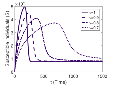
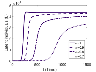
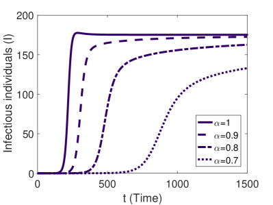
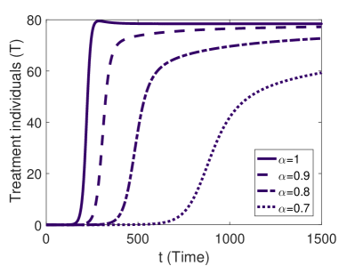
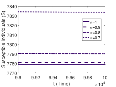
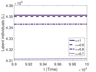
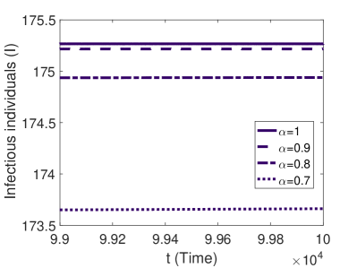
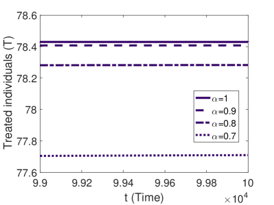
In this section we study the dynamical behavior of our model (3.1), by variation of the noninteger order derivative $\alpha$. The parameter values used in the simulations can be found in Table 1, with exception of $b=0.0005$, which we changed in order to get a value of $R_{0}$ bigger than one (endemic situation). Direct calculations, with these parameter values, give $R_{0}=7.1343>1$ and the endemic equilibrium

$$E^{*}=(7779.3,43512,175.2,78.4).$$

We consider the initial conditions

$$S(0)=0.8,\quad L(0)=0.05,\quad I(0)=0.1,\quad T(0)=0.05$$ (5.1)

and a fixed time step size of $h=2^{-8}$.

Table 1. Parameter values taken from Yang201079 .

Parameter	Description	Value
$\Lambda$	Recruitment rate	792.8571
$\beta$	Transmission coefficient	$5\times 10^{-5}$
$\mu$	Natural death rate	$0.143$
$k$	Treatment failure rate	$0.15$
$\delta$	Rate at which treated individuals leave the $T$ compartment	$1.5$
$\epsilon$	Rate at which latent individuals $L$ become infectious	$0.00368$
$\gamma$	Treatment rate for infectious individuals $I$	$0.7$
$\alpha_{1}$	TB-induced death rate for infectious individuals $I$	$0.3$
$\alpha_{2}$	TB-induced death rate for under treatment individuals $T$	$0.05$

For the numerical implementation of the fractional derivatives, we have used the Adams–Bashforth–Moulton scheme, which has been implemented in the Matlab code fde12 by Garrappa Garrappa . Regarding convergence and accuracy of the numerical method, we refer to [2] . The stability properties of the method implemented by fde12 have been studied in [5] . We consider, without loss of generality, the fractional-order derivatives $\alpha=1.0,0.9,0.8$ and $0.7$. In Figures 1–2, one can see that when $\alpha\rightarrow 1$ the solutions of our model converge to the solutions obtained in Yang201079 . The simulation results confirm, numerically, the stability result of Theorem 4.

Figure 1. Numerical simulation of the Caputo TB system (3.1) with values as in Table 1, with exception of $b=0.0005$, and initial conditions (5.1).

Figure 2. Numerical simulation of the Caputo TB system with parameters and initial conditions as in Fig. 1, showing that the solutions converge to the endemic equilibrium $(7779.3,43512,175.2,78.4)$ for $\alpha=1$.

6. Conclusions

In this work we proposed a Caputo fractional-order tuberculosis (TB) model. Existence of equilibrium points has been investigated and the uniform asymptotic stability of the unique endemic equilibrium proved via a suitable Lyapunov function. Our analytical results were complemented by numerical simulations in Matlab, illustrating the obtained stability result. The proposed fractional order model provides richer and more flexible results when compared with the corresponding integer-order TB model.

This research was partially supported by the Portuguese Foundation for Science and Technology (FCT) through the R&D unit CIDMA, reference UID/MAT/04106/2013, and by project PTDC/EEI-AUT/2933/2014 (TOCCATA), funded by FEDER funds through COMPETE 2020 – Programa Operacional Competitividade e Internacionalização (POCI) and by national funds through FCT. Silva is also grateful to the FCT post-doc fellowship SFRH/BPD/72061/2010; Wojtak to the FCT PhD fellowship PD/BD/128183/2016.

References

- [1] E. Ahmed, A. S. Elgazzar. On fractional order differential equations model for nonlocal epidemics. Physica A: Statistical Mechanics and Its Applications 379 (2007), no. 2, 607–614.
- [2] E. Ahmed, A. M. El-Sayed, H. A. El-Saka. Equilibrium points, stability and numerical solutions of fractional-order predator-prey and rabies models. J. Math. Anal. Appl. 325 (2007), no. 1, 542–553.
- [3] A. Atangana. Application of Fractional Calculus to Epidemiology. In: Fractional dynamic, Chapt. 11, De Gruyter Open, Ed.: C. Cattani, H. M. Srivastava, X. Yang, 174–190, 2015.
- [4] D. Baleanu, S. J. Sadati, R. Ghaderi, A. Ranjbar, T. Abdeljawad, F. Jarad. Razumikhin stability theorem for fractional systems with delay. Abstr. Appl. Anal. 2010 (2010), Art. ID 124812, 9 pp.
- [5] L. Bourdin, T. Odzijewicz, D. F. M. Torres. Existence of minimizers for generalized Lagrangian functionals and a necessary optimality condition–application to fractional variational problems. Differential Integral Equations 27 (2014), no. 7-8, 743–766. arXiv:1403.3937
- [6] F. Brauer. Mathematical epidemiology: Past, present, and future. Infectious Disease Modelling 2 (2017) 113–127.
- [7] M. Caputo. Linear Models of Dissipation whose Q is almost Frequency Independent-II. Geophysical Journal of the Royal Astronomical Society 13 (1967), no. 5, 529–539.
- [8] L. Chen, Y. He, Y. Chai, R. Wu. New results on stability and stabilization of a class of nonlinear fractional-order systems. Nonlinear Dyn. 75 (2014), no. 4, 633–641.
- [9] A. Debbouche, D. F. M. Torres. Approximate controllability of fractional delay dynamic inclusions with nonlocal control conditions. Appl. Math. Comput. 243 (2014) 161–175. arXiv:1405.6591
- [10] H. Delavari, D. Baleanu, J. Sadati. Stability analysis of Caputo fractional-order nonlinear systems revisited. Nonlinear Dyn. 67 (2012), no. 4, 2433–2439.
- [11] R. Denysiuk, C. J. Silva, D. F. M. Torres. Multiobjective approach to optimal control for a tuberculosis model. Optim. Methods Softw. 30 (2015), no. 5, 893–910. arXiv:1412.0528
- [12] K. Diethelm. The Analysis of Fractional Differential Equations: An Application-Oriented Exposition using Differential Operators of Caputo Type. Springer-Verlag, Berlin, 2010.
- [13] K. Diethelm, N. J. Ford, A. D. Freed. Detailed error analysis for a fractional Adams method. Numer. Algorithms 36 (1) (2004) 31–52.
- [14] Y. Ding, H. Ye. A fractional-order differential equation model of HIV infection of T-cells. Math. Comput. Modelling 50 (2009), no. 3-4, 386–392.
- [15] R. Garrappa. On linear stability of predictor-corrector algorithms for fractional differential equations. Internat. J. Comput. Math. 87 (2010), no. 10, 2281–2290.
- [16] R. Garrappa. Predictor-corrector PECE method for fractional differential equations. MATLAB Central File Exchange, File ID: 32918, 2011.
- [17] G. González-Parra, A.J. Arenas, B.M. Chen-Charpentier. A fractional order epidemic model for the simulation of outbreaks of influenza A(H1N1). Math. Meth. Appl. Sci. 37 (2014), no. 15, 2218–2226.
- [18] S. Jahanshahi, E. Babolian, D. F. M. Torres, A. Vahidi. Solving Abel integral equations of first kind via fractional calculus. J. King Saud Univ. Sci. 27 (2015), no. 2, 161–167. arXiv:1409.8446
- [19] Y. Li, Y.Q. Chen, I. Podlubny. Mittag–Leffler stability of fractional order nonlinear dynamic systems. Automatica 45 (2009), 1965–1969.
- [20] Y. Li, Y.Q. Chen, I. Podlubny. Stability of fractional-order nonlinear dynamic systems: Lyapunov direct method and generalized Mittag-Leffler stability. Comput. Math. Appl. 59 (2010), 1810–1821.
- [21] C. Li, Y. Ma. Fractional dynamical system and its linearization theorem. Nonlinear Dyn. 71 (2013), 621–633.
- [22] C. P. Li, F. R. Zhang. A survey on the stability of fractional differential equations. Eur. Phys. J. Special Topics 193 (2011), 27–47.
- [23] A. B. Malinowska, T. Odzijewicz, D. F. M. Torres. Advanced methods in the fractional calculus of variations. SpringerBriefs in Applied Sciences and Technology. Springer, Cham, 2015.
- [24] A. B. Malinowska, D. F. M. Torres. Introduction to the fractional calculus of variations. Imperial College Press, London, 2012.
- [25] D. Matignon. Stability result on fractional differential equations with applications to control processing. In: IMACS-SMC Proceedings, Lille, France, July, 963–968, 1996.
- [26] I. Petráš. Stability of fractional-order systems with rational orders: a survey. Fract. Calc. Appl. Anal. 12 (2009), no. 3, 269–298.
- [27] I. Petráš. Fractional-Order Nonlinear Systems: Modelling, Analysis and Simulation. Springer, Dordrecht, 2011.
- [28] C. M. A. Pinto, J. A. T. Machado. Fractional model for malaria transmission under control strategies. Comput. Math. Appl. 66 (2013), 908–916.
- [29] I. Podlubny. Fractional Differential Equations. Academic Press, San Diego, 1999.
- [30] S. Pooseh, H. S. Rodrigues, D. F. M. Torres. Fractional derivatives in Dengue epidemics. AIP Conf. Proc. 1389 (2011), no. 1, 739–742. arXiv:1108.1683
- [31] M. Rivero, S. V. Rogosin, J. A. T. Machado, J. J. Trujillo. Stability of fractional order systems. Math. Probl. Eng. 2013 (2013), Art. ID 356215, 14 pp.
- [32] D. Rocha, C. J. Silva, D. F. M. Torres. Stability and optimal control of a delayed HIV model. Math. Methods Appl. Sci., in press. DOI:10.1002/mma.4207 arXiv:1609.07654
- [33] P. Rodrigues, C. J. Silva, D. F. M. Torres. Cost-effectiveness analysis of optimal control measures for tuberculosis. Bull. Math. Biol. 76 (2014), no. 10, 2627–2645. arXiv:1409.3496
- [34] C. J. Silva, H. Maurer, D. F. M. Torres. Optimal control of a Tuberculosis model with state and control delays. Math. Biosci. Eng. 14 (2017), no. 1, 321–337. arXiv:1606.08721
- [35] C. J. Silva, D. F. M. Torres. Optimal control strategies for tuberculosis treatment: a case study in Angola. Numer. Algebra Control Optim. 2 (2012), no. 3, 601–617. arXiv:1203.3255
- [36] C. J. Silva, D. F. M. Torres. Optimal control for a tuberculosis model with reinfection and post-exposure interventions. Math. Biosci. 244 (2013), no. 2, 154–164. arXiv:1305.2145
- [37] C. J. Silva, D. F. M. Torres. Optimal control of Tuberculosis: A review. In: J. P. Bourguignon et al. (eds.), Dynamics, Games and Science, CIM Series in Mathematical Sciences 1, Springer, 2015, 701–722. arXiv:1406.3456
- [38] C. J. Silva, D. F. M. Torres. Global stability for a HIV/AIDS model. Commun. Fac. Sci. Univ. Ank. Ser. A1 Math. Stat. 67 (2018), no. 1, 93–101. arXiv:1704.05806
- [39] N. H. Sweilama, S. M. AL-Mekhlafib. Numerical study for multi-strain tuberculosis (TB) model of variable-order fractional derivatives. J. Adv. Res. 7 (2016), no. 2, 271–283.
- [40] J. C. Trigeassou, N. Maamri, J. Sabatier, A. Oustaloup. A Lyapunov approach to the stability of fractional differential equations. Signal Process. 91 (2011), no. 3, 437–445.
- [41] C. Vargas-De-León. Volterra-type Lyapunov functions for fractional-order epidemic systems. Commun. Nonlinear Sci. Numer. Simulat. 24 (2015), 75–85.
- [42] WHO. Global tuberculosis report 2016. World Health Organization, 2016.
- [43] Y. Yang, J. Li, Z. Ma, L. Liu. Global stability of two models with incomplete treatment for tuberculosis. Chaos, Solitons & Fractals 43 (2010), 79–85.
- [44] L. Zhang, G. Huang, A. Liu, R. Fan. Stability Analysis for a Fractional HIV Infection Model with Nonlinear Incidence. Discrete Dyn. Nat. Soc. 2015 (2015), Art. ID 563127, 11 pp.