Dynamics of marginally trapped surfaces in a binary black hole merger: Growth and approach to equilibrium

Abstract

The behavior of quasi-local black hole horizons in a binary black hole merger is studied numerically. We compute the horizon multipole moments, fluxes and other quantities on black hole horizons throughout the merger. These lead to a better qualitative and quantitative understanding of the coalescence of two black holes; how the final black hole is formed, initially grows and then settles down to a Kerr black hole. We calculate the rate at which the final black hole approaches equilibrium in a fully non-perturbative situation and identify a time at which the linear ringdown phase begins. Finally, we provide additional support for the conjecture that fields at the horizon are correlated with fields in the wave-zone by comparing the in-falling gravitational wave flux at the horizon to the outgoing flux as estimated from the gravitational waveform.

I Introduction

Gravitational wave signals from binary black hole merger events are now routinely computed in numerical simulations. For generic spin configurations and at least for moderate mass ratios, various aspects of the problem are well understood; this includes the initial data, numerical methods, gauge conditions for the evolution, locating black hole horizons, and finally extracting gravitational wave signals in the wave zone. We refer the reader to Pretorius (2005); Campanelli et al. (2006); Baker et al. (2006) which demonstrated the first successful binary black hole simulations and to e.g. Baumgarte and Shapiro (2010); Shibata (2016); Alcubierre (2008) for further details and references.

What is somewhat less well understood is the behavior of black hole horizons near the merger. For example, it is clear from the black hole area increase law that as soon as the final black hole is formed, its area will increase and it will eventually asymptote to a higher value. It is also expected that the rate of area increase will be largest immediately when the common horizon is formed which is when the in-falling gravitational radiation has the largest amplitude and the effects of non-linearities cannot be neglected. At a somewhat later time, the rate of area increase will slow down and the problem can be treated within black hole perturbation theory. Unanswered questions include: What is the angular distribution of the gravitational wave flux entering the horizon and causing it to grow? What is the rate of decrease of this flux with time? Is it possible to identify a time, purely based on the properties of the horizon, after which the flux is small enough that we can trust the results of perturbation theory?

A different but related set of questions arises with the approach to Kerr. Mass and spin multipole moments of black hole horizons can be constructed Ashtekar et al. (2004, 2013). These multipole moments describe the instantaneous intrinsic geometry of the black hole at any given time. The first mass multipole moment is just the mass, while the first non-zero spin multipole moment for a regular horizon is just the angular momentum. For a Kerr black hole, these lowest multipole moments determine uniquely all of the higher moments. For the dynamical black hole, the higher moments can be computed independently in the numerical simulation and we can extract the rate at which the multipole moments approach their Kerr values. Some of the above questions were considered in Schnetter et al. (2006) but numerical relativity has made great progress since then and it is useful to revisit these issues again. We shall use the framework of quasi-local horizons for our analysis; see e.g. Ashtekar and Krishnan (2004); Booth (2005) for reviews.

Another question we wish to address is that of when the gravitational waveform can be considered to be in the ringdown phase. In principle, by fitting the final part of the waveform with damped sinusoids we can extract the frequency $f$ and damping time $\tau$ of the black hole ringdown mode(s), thereby allowing a test of the Kerr nature of the final black hole proposed in Dreyer et al. (2004) if we can observe more than a single mode. However, it is non-trivial to know at what point one should start fitting the damped sinusoid. If we start too close to the merger, incorrect values of $(f,\tau)$ can be obtained. An example of this issue appears in the ringdown analysis of the binary black hole detection GW150914 Abbott et al. (2016). As demonstrated in Fig. 5 of Abbott et al. (2016), choosing different start-times for fitting a damped sinusoid to the post-merger phase of the observed strain data has a noticeable effect on the recovered values of the frequency and damping time, and thus also on the inferred values of the mass and angular momentum of the final black hole. Similar questions have been studied recently in Thrane et al. (2017); Bhagwat et al. (2017); Cabero et al. (2017). It is then natural to ask whether one can use correlations with the horizon to quantitatively provide a time in the waveform beyond which the ringdown analysis is valid. We shall use the multipole moments to address this question.

Finally, for vacuum general relativity, the behavior of spacetime at or near the horizon is correlated with what happens in the wave zone and the gravitational waveform. This notion was discussed in a series of papers by Jaramillo et al. Jaramillo et al. (2012a, b, 2011a) and used to explain the phenomenon of anti-kicks, a short phase of deceleration which reduces the kick-velocity of the final black hole remnant Rezzolla et al. (2010). The basic idea is quite simple: in an initial value formulation of general relativity, the initial data fields at early times outside the horizon determine both the behavior of the horizon and also the waveform far away from the horizon. Thus, if the in- and out-going modes are coupled (as they most likely are due to the non-linearities of general relativity), there must be correlations between data on the horizon and the gravitational waveform. This applies also to fields on apparent horizons which are inside the event horizon. As expected the black hole horizon is not a source for the gravitational waveform and of course cannot causally influence any observations in the wave zone. However, correlations due to a common source could provide a way to extract information about the near horizon spacetime from gravitational wave observations. A similar suggestion was also made in Section 8 of Ashtekar and Krishnan (2004): the radiation trapped between the horizon and the peak of the effective gravitational potential outside the black hole could fall into the horizon thereby increasing its area, and also cause the black hole horizon to lose its irregularities. This apparently simple conjecture is not yet fully developed. For example, it could be possible that such correlations do not exist for generic initial data but are instead a special property of astrophysical initial data where one wants to minimize incoming radiation from past null infinity. Here we shall provide additional support to this conjecture by showing that the outgoing flux obtained from the gravitational signal is highly correlated with the in-falling flux at the horizon.

The plan for the rest of the paper is as follows. Section II briefly reviews basic notions and equations for dynamical horizons and the numerical simulations. Section III describes various dynamical horizon quantities computed numerically in a binary black hole simulation providing a better qualitative and quantitative understanding of binary black hole coalescence. This section also illustrates the area increase law starting with the initial black hole and ending with the final black hole. It is unclear whether or not there is a connected sequence of marginally trapped surfaces that take us from the initial black holes to the final one. If in fact there is such a sequence of marginally trapped surfaces, we could track the area of the black hole through the merger. Sec. IV studies the horizon multipole moments and the rate at which they approach their equilibrium Kerr values. We identify an epoch about $10M$ after the formation of the common horizon when there is an evident change in the decay rate of the moments. Section V carries out the cross-correlation study between the horizon fluxes with the waveform (or more precisely, with the outgoing luminosity). This provides the critical link between properties of spacetime in the strong field region and gravitational wave observations. Section VI presents concluding remarks and lists some open problems.

II Preliminaries

II.1 Basic properties of dynamical horizons

We begin by briefly summarizing basic definitions of marginally trapped surfaces and dynamical horizons for later use. Let $\mathcal{S}$ be a closed spacelike surface with topology $S^{2}$. Denote the out- and in-going future directed null normals to $\mathcal{S}$ by $\ell^{a}$ and $n^{a}$ respectively. We require that $\ell\cdot n=-1$. We are allowed to scale $\ell^{a}$ and $n^{a}$ by positive definite functions $f$ such that $\ell^{a}\rightarrow f\ell^{a}$ and $n^{a}\rightarrow f^{-1}n^{a}$, thus preserving $\ell\cdot n$. Let $q_{ab}$ be the intrinsic 2-metric on $\mathcal{S}$ obtained by restricting the spacetime metric to $\mathcal{S}$. The expansions of $\ell^{a}$ and $n^{a}$ are defined as

$$\Theta_{(\ell)}=q^{ab}\nabla_{a}\ell_{b}\,,\qquad\Theta_{(n)}=q^{ab}\nabla_{a}n_{b}\,.$$ (1)

$\mathcal{S}$ is said to be a marginally outer trapped surface (MOTS) if $\Theta_{(\ell)}=0$. In addition, $\mathcal{S}$ is said to be a (future-outer) marginally trapped surface if $\Theta_{(n)}<0$. MOTSs are used to conveniently locate black holes in numerical simulations Thornburg (2004). This can be done on every time slice, and does not require knowledge of the full spacetime.

Under certain general stability conditions, it can be shown that marginally trapped surfaces evolve smoothly under time evolution Andersson et al. (2005, 2009, 2008). Apparent horizons are the outermost marginally outer trapped surfaces on a given spatial slice and the outermost condition can cause apparent horizons to jump discontinuously as new marginally trapped surfaces are formed. However, the underlying marginally trapped surfaces continue to evolve smoothly. We shall describe this behavior in greater detail later in this paper. Even the marginally trapped surfaces which are not expected to satisfy the stability conditions are found empirically to evolve smoothly thus a more general result might hold for the time evolution Booth et al. (2017).

Given the smooth time evolution, we can consider the sequence $\mathcal{S}_{t}$ of marginally outer trapped surfaces at various times $t$ and construct the 3-dimensional tube obtained by stacking up all the $\mathcal{S}_{t}$. This leads us to the definition of a marginally trapped tube (MTT) as a 3-surface foliated by marginally outer trapped surfaces. Let $\mathcal{H}$ denote the MTT, and let $A_{t}$ be the area of $\mathcal{S}_{t}$. There are three cases of interest depending on whether $\mathcal{H}$ is spacelike, null or timelike. When $\mathcal{H}$ is spacelike, and $\Theta_{(n)}<0$, it is called a dynamical horizon Ashtekar and Krishnan (2002, 2003, 2004). In this case, its area increases monotonically in the outward direction. More generally, this also holds if the average of $\Theta_{(n)}$ over $\mathcal{S}_{t}$ is negative. If $\widehat{r}^{a}$ is the unit normal (outward pointing) to $\mathcal{S}_{t}$ on $\mathcal{H}$, and $\widehat{\tau}^{a}$ is the future directed unit timelike normal to $\mathcal{H}$, we can construct the out- and in-going null normals

$$\ell^{a}=\frac{\widehat{\tau}^{a}+\widehat{r}^{a}}{\sqrt{2}}\,,\quad n^{a}=\frac{\widehat{\tau}^{a}-\widehat{r}^{a}}{\sqrt{2}}\,.$$ (2)

It then follows that

$$\mathcal{L}_{\widehat{r}}\widetilde{\epsilon}_{ab}=-\frac{1}{\sqrt{2}}\Theta_{(n)}\widetilde{\epsilon}_{ab}\,,$$ (3)

where $\widetilde{\epsilon}_{ab}$ is the volume 2-form on $\mathcal{S}_{t}$. Integrating this equation over $\mathcal{S}_{t}$ shows that the area increases along $\widehat{r}^{a}$ if the average of $\Theta_{(n)}$ on $\mathcal{S}_{t}$ is negative.

When $\mathcal{H}$ is null the areas of its cross-sections $\mathcal{S}_{t}$ are constant, and is known as an isolated horizon (see e.g. Ashtekar et al. (2000a, 1999, b, 2001, 2002) for details and precise definitions). When $\mathcal{H}$ is timelike and $\Theta_{(n)}<0$, the area of its cross-sections decreases to the future and is called a timelike membrane. Timelike MTTs appear in numerical simulations as well (but they are not the outermost marginally outer trapped surfaces). The reader is referred to Ashtekar and Krishnan (2004); Booth (2005); Krishnan (2014) for reviews. See e.g. Ben-Dov (2004); Booth et al. (2006) for examples of MTTs of various signatures; see also Chu et al. (2011) for other numerical studies of inner and outer horizons.

For a dynamical horizon, we can in fact do better than just showing that the area increases. As at null infinity, we can obtain an explicit positive-definite expression for the flux of gravitational radiation crossing a dynamical horizon. This is a non-trivial fact which does not hold for arbitrary surfaces, and it emphasizes again the special properties of a dynamical horizon Ashtekar and Krishnan (2002, 2003, 2004). To discuss this further we need a few more definitions. The shear $\sigma_{ab}$ of $\ell^{a}$ will play an important role and it is defined as:

$$\sigma_{ab}={q_{a}}^{c}{q_{b}}^{d}\nabla_{c}\ell_{d}-\frac{1}{2}\Theta_{(\ell)}q_{ab}\,.$$ (4)

Let $h_{ab}$ be the 3-metric on $\mathcal{H}$ and as before let $\widehat{r}^{a}$ be the outward pointing unit spacelike normal to $\mathcal{S}_{t}$ on $\mathcal{H}$. Define a one-form $\zeta_{a}$ on $\mathcal{H}$ as $\zeta_{a}={h_{a}}^{b}\widehat{r}^{c}\nabla_{c}\ell_{b}$. The instantaneous gravitational energy flux is an integral of a quantity $\mathfrak{f}$ over marginally trapped surfaces $\mathcal{S}_{t}$:

$$\mathfrak{f}=\frac{1}{2}\sigma_{ab}\sigma^{ab}+\zeta_{a}\zeta^{a}\,.$$ (5)

$\mathfrak{f}$ is the energy flux per unit area and per unit time entering the horizon (with the area radius of $\mathcal{S}_{t}$ playing the role of “time” on the horizon); note the different normalization of $\ell\cdot n$ compared to Ashtekar and Krishnan (2004). This is an exact expression in full general relativity with no approximations. It satisfies the expected properties of gravitational radiation, for example it is manifestly positive and it vanishes in spherical symmetry. No such local expression is possible for the event horizon in general. This is because of the global properties of the event horizon; there are well known examples where the event horizon grows in flat space where there cannot be any non-zero local flux Ashtekar and Krishnan (2004). There do exist flux formulae for the growth of the event horizon in perturbative situations. In Hawking and Hartle (1972) it is found that the rate of area increase for an event horizon is approximately proportional to the integral of $|\sigma|^{2}$ with $\sigma$ being the shear of the null generator of the event horizon. This however only holds within perturbation theory and furthermore, because of the nature of the event horizon, this really only makes sense when the end state of the event horizon is known or assumed. See Booth and Fairhurst (2007) for a more detailed comparison with Hawking and Hartle (1972).

The other ingredient we shall use frequently in this paper are the multipole moments. These were first introduced in Ashtekar et al. (2004) for isolated horizons, and extended and used in Schnetter et al. (2006) for dynamical horizons. These multipole moments have found applications in, for example, predictions of the anti-kick in binary black hole mergers Rezzolla et al. (2010) and for studying tidal deformations of black holes Cabero and Krishnan (2015); Gürlebeck (2015). The work by Ashtekar et al. Ashtekar et al. (2013) provides flux formulae for the multipole moments and a procedure for choosing a suitable class of time evolution vector fields on a dynamical horizon. Here we shall use them to study the approach of a dynamical horizon to equilibrium.

Our investigation of dynamical horizons will be informed by exact results for axisymmetric isolated horizons $\mathcal{H}$. Every cross-section of an isolated horizon with spherical topology has the same area $A$. Let $\ell^{a}$ be a null generator of $\mathcal{H}$ and $\varphi^{a}$ the axial symmetry vector field. For an isolated horizon it can be shown that the Weyl tensor component $\Psi_{2}$ at the horizon is time independent. On every cross-section $\mathcal{S}$ it is given by

$$\Psi_{2}=\frac{\mathcal{R}}{4}+\frac{i}{2}{}^{\star}d\omega\,.$$ (6)

Here $\mathcal{R}$ is the two-dimensional scalar curvature of $\mathcal{S}$, ^⋆ denotes the Hodge-dual, and $\omega$ is a 1-form on $\mathcal{H}$ defined by

$$V^{a}\nabla_{a}\ell_{b}=V^{a}\omega_{a}\ell_{b}\,$$ (7)

with $V^{a}$ being any vector field tangent to $\mathcal{H}$. The surface gravity is $\kappa_{\ell}:=\omega_{a}\ell^{a}$. The angular momentum of $\mathcal{H}$ is given by

$$J_{\mathcal{S}}=-\frac{1}{8\pi}\oint_{\mathcal{S}}\omega_{a}\varphi^{a}\,d^{2}S\,.$$ (8)

Let $\Sigma$ be a spatial Cauchy surface which intersects $\mathcal{H}$, and let $\mathcal{S}=\mathcal{H}\cap\Sigma$. It turns out that $\omega_{a}\varphi^{a}=K_{ab}\widehat{R}^{a}\varphi^{a}$ where $K_{ab}$ is the extrinsic curvature of $\Sigma$ and $R^{a}$ the unit spacelike normal to $\mathcal{S}$ on $\Sigma$ Dreyer et al. (2003). We will use this exact result for isolated horizons to also define angular momentum for cross-sections of dynamical horizons, since $K_{ab}$ is readily available in any numerical simulation based on a 3+1 formulation of general relativity. Given the angular momentum, the horizon mass is then defined by

$$M_{\mathcal{S}}=\frac{1}{2R_{\mathcal{S}}}\sqrt{R_{\mathcal{S}}^{4}+4J_{\mathcal{S}}^{2}}\,,$$ (9)

with $R_{\mathcal{S}}=\sqrt{A/4\pi}$ being the area-radius of $\mathcal{S}$.

The symmetry vector $\varphi^{a}$ can be used to construct a preferred coordinate system $(\theta,\varphi)$ on $\mathcal{S}$ analogous to the usual spherical coordinates on a sphere. We can then use spherical harmonics in this preferred coordinate system to construct multipole moments. As expected we have two sets of moments $M_{n}$, $J_{n}$ such that $M_{0}$ is the mass $M_{\mathcal{S}}$ and $J_{1}$ is the angular momentum $J_{\mathcal{S}}$. Moreover, $\mathcal{R}$ and $\omega_{a}$ can be thought of as being (proportional to) the surface mass density and surface current on $\mathcal{S}$ respectively Ashtekar et al. (2005). This leads us to the following expressions for the multipole moments:

$$M_{n}=\frac{M_{\mathcal{S}}R_{\mathcal{S}}^{n}}{8\pi}\oint_{S}\mathcal{R}P_{n}(\zeta)d^{2}S\,,$$ (10)

and

$$J_{n}=\frac{R_{\mathcal{S}}^{n-1}}{8\pi}\oint_{S}P_{n}^{\prime}(\zeta)K_{ab}\varphi^{a}R^{b}d^{2}S\,.$$ (11)

Here $P_{n}(\zeta)$ is the $n^{\mathrm{th}}$ Legendre polynomial, $P_{n}^{\prime}(\zeta)$ its derivative and $\zeta=\cos\theta$.

For a dynamical horizon, many of the above assumptions do not hold. For example, $\Psi_{2}$ is not time independent and neither are the area, curvature other geometric quantities on $\mathcal{S}_{t}$. However, following Schnetter et al. (2006), we shall continue to interpret the surface density and current in the same way so that the multipole moments share the same definitions as above. These multipole moments are gauge independent in the same sense as a dynamical horizon is gauge independent, i.e. it exists as a geometric object in spacetime independent of the spacetime foliation used to locate it. A different choice of spacetime slicing will give a different dynamical horizon, but for any given dynamical horizon, the multipole moments are gauge independent.

An important issue is the choice of $\varphi^{a}$. When the common horizon is formed, it is highly distorted and it will generally not be even approximately axisymmetric. For this reason, while there exist various methods for finding approximate axial Killing vectors Cook and Whiting (2007); Owen (2007); Lovelace et al. (2008); Beetle (2008); Dreyer et al. (2003); Beetle and Wilder (2014), in our opinion it is not fruitful to try and apply these to the newly formed common horizon such as the ones we have here. Since we shall restrict ourselves to the case of the merger of equal mass non-spinning black holes where the orbital angular momentum provides a natural orientation, the kick velocity for the final black hole vanishes, and the spacetime has reflection symmetry. This initial configuration is physically relevant since all gravitational wave events observed from binary black hole mergers so far are consistent with being comparable mass systems of initially non-spinning black holes. We shall therefore align the z-axis with the orbital angular momentum and simply take $\varphi^{a}$ to be $\partial_{\phi}$, i.e. defined by the z-axis. The presence of reflection symmetry across the equator makes this a natural (though of course not unique) choice as well. For more general initial configurations, we expect the approach suggested in Ashtekar et al. (2013) to be useful since it relies only on the end-state being axisymmetric with an axial symmetry vector $\varphi^{a}$ and it provides a method of transporting $\varphi^{a}$ to all points on the dynamical horizon. This will be implemented in forthcoming work.

II.2 Numerical simulations of binary black hole mergers

II.2.1 Physical setup

We employ a full numerical simulation to generate a binary black hole spacetime geometry. As we are interested only in the merger and ringdown phases of a binary black hole merger, we start our simulation shortly before the merger, choosing the so-called QC-0 initial conditions Baker et al. (2002); Cook (1994) for simplicity. These correspond to an equal-mass non-spinning binary black hole system in its last orbit before coalescence.

The QC-0 system has an ADM mass $M_{\mathrm{ADM}}\approx 1.00788\,M$, where $M$ is the (arbitrarily chosen) mass unit in the simulation. Compared to calculations that track several orbits of the inspiral phase, the main difference of our setup is that it does not give us access to the inspiral waveform, and that we do not know the eccentricity that the QC-0 would have had during inspiral. We list the QC-0 system parameters in table 1.

Parameter	Symbol	Value
half separation	$b$	$1.168642873$
puncture mass	$m^{+}$	$0.453$
puncture mass	$m^{-}$	$0.453$
puncture momentum	$p^{+}_{y}$	$+0.3331917498$
puncture momentum	$p^{-}_{y}$	$-0.3331917498$
total mass	$M_{\mathrm{ADM}}$	$1.00788$

Table 1: QC-0 system parameters

We track the two individual apparent horizons, and we find that the system performs about three quarters of an orbit before a common apparent horizon forms. We locate both the outer and the inner common apparent horizons (see e.g. figure 1), and by comparing the shapes and areas of the common horizons we verify that the common horizons form a single smooth world tube, and that we detect this common horizon immediately as it appears in our spacetime foliation. After coalescence, the outer common horizon quickly settles down to a stationary state within about $10\,M$. Due to the chosen gauge conditions and numerical resolutions, we lose track of the individual and the inner common horizon about $5\,M$ after coalescence. This shall be explained in greater detail shortly.

II.2.2 Numerical details

We solve the Einstein equations via the Einstein Toolkit Löffler et al. (2012); EinsteinToolkit in their BSSN formulation Alcubierre et al. (2000, 2003); Brown et al. (2009) using the usual $1+\log$ slicing and $\Gamma$-driver shift conditions.

We set up initial conditions via the puncture method Ansorg et al. (2004). We locate apparent horizons via the method described in Thornburg (1996, 2004). The algorithms to evaluate quantities for isolated and dynamical horizons were previously described in Dreyer et al. (2003) and Schnetter et al. (2006).

We use a domain with an outer boundary at $240\,M$, making use of the reflection symmetry about the $z=0$ plane and the equal mass $\pi$-rotation symmetry about the $z$ axis for a domain extent of $[0;240]\times[-240;240]\times[0;240]$. We employ adaptive mesh refinement (AMR), tracking the individual and outer common horizon, and placing a stack of progressively refined regions around these. For completeness, we list our evolution parameters in table 2.

Parameter	Symbol	Value
$1+\log$	$n$	$1$
$1+\log$	$f$	$2$
$\Gamma$-driver	$\eta$	$0.75$
$\Gamma$-driver	$F$	$0.75\cdot\alpha$
domain radius		$240$
AMR levels		$7$ total
indiv. BH AMR level radii		$[32,16,8,4,2,1]$
common BH AMR level radii		$[64,32,16,8,4,2]$
finest resolution	$\Delta x$	$0.015625$
horizon surface resolution	$\Delta\theta$	$0.02936\,\mathrm{rad}$
horizon surface resolution	$\Delta\phi$	$0.02909\,\mathrm{rad}$

Table 2: Evolution parameters

III The area increase law

While this paper is mainly concerned with the properties of the final horizon and its approach to equilibrium, it is interesting to start with a somewhat different issue, namely to understand the various kinds of horizons present in a binary black hole system and how their areas evolve. In particular we shall track the areas, coordinate shapes and some other physical properties of the horizon areas starting from the two initial horizons right up to when the final horizon reaches equilibrium. These questions were also studied in Schnetter et al. (2006), but with much better numerics we are now able to evolve through the merger al the way to the equilibrium state at late times.

As mentioned earlier, the common apparent horizon forms at about $t\approx 18.656M$ in the simulation time. The common horizon splits into inner and outer components. The areas are shown in Fig. 1. The outer horizon continues to grow while the inner horizon shrinks. The areas of the two individual horizons are seen to remain essentially constant.

Figure 1: This figure shows, as a function of time, the areas of the common-outer and inner horizons, and the sum of the areas of the two individual horizons. The common horizon first appears at the intersection of the green and blue curves which then splits into an inner (blue) and outer (green) horizon. The area of the inner horizon decreases in area while the outer horizon increases and eventually reaches an equilibrium value. The purple curve refers to the sum of the areas of the two separate individual horizons. We have plotted only up to $t=50M$ since the area of the common-outer horizon after that point is essentially constant. The small dip in the area of the individual horizons at the end indicates a problem with numerical accuracy for locating the inner horizon, and is not to be trusted at that point.

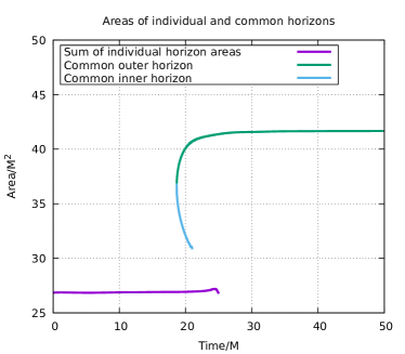
Fig. 1 leads us to conjecture that there could be a 3-dimensional marginally trapped tube that interpolates between the two initial horizons and the final outer marginally trapped tube. For this to happen, the curve in Fig. 1 for the individual horizons must join with the curve for the inner common horizon whose area is rapidly decreasing. If this were to happen, we could obtain the area as a monotonic function on the smooth three dimensional surface: start as usual by tracking the individual horizons going forward in time. At the point that merger with the common-inner horizon happens, then we would continue going backwards in time so that the area is still increasing. Finally, as can be seen in Fig. 1, this joins smoothly with the common-outer horizon which increases in area going forward in time, and eventually reaches equilibrium.

Our numerical simulations are not able to track the inner common horizon beyond $t\approx 21M$ because it becomes highly distorted and is most likely not a star shaped surface at that time in our simulation . Other simulations have successfully followed the evolution of the two individual binary marginally trapped surfaces for a somewhat longer time Mösta et al. (2015) where it was shown that the two marginally trapped surfaces can penetrate each other. Although we are able to follow the two individual horizons somewhat longer than the inner common horizon, again because of technical issues we are not able to follow them to the point where they penetrate each other.

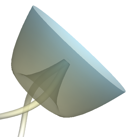
The further evolution of both the common inner horizon and the binary horizons is still unresolved, although it is likely that at some point they join together. The theorems that guarantee smooth time evolution of marginally trapped surfaces do not apply in this case because the general stability conditions do not hold for inner horizons. However, two main possibilities seem likely. Either, after penetrating one another the two binary horizons merge together, and then subsequently merge with the inner horizon. Or, the two horizons merge with the inner horizon after penetration, but before becoming a single horizon. An artistic impression (not based on actual data) for the second possibility is displayed in Fig. 2.

If either case were confirmed to be true, one could then introduce a parameter $\lambda$ along the continuous 3-dimensional surface and the area $A(\lambda)$ would be a monotonically increasing function starting from the individual horizons to the final outer horizon which eventually reaches equilibrium. It would be of interest to find a suitable gauge condition which would enable us to track the inner common-horizon to confirm or disprove this scenario.

Figure 2: A speculative scenario for the fate of the two individual and the common-inner horizons. After the common outer and inner horizons form, the initial horizons continue to orbit, eventually intersecting with one another and then merging with the common inner horizon. Current horizon tracking algorithms are unable to track the individual horizons this far into the evolution because of the high level of horizon distortion and this scenario remains speculation. The plot is not drawn to scale.

The other feature that is obvious from Fig. 1 is the fact that the areas of the two individual horizons are essentially constant even though the start of our simulation is already very close to the merger. Only the sum of their areas is shown in Fig. 1 but, since we are working with equal mass non-spinning black holes, the two areas are the same. There might be interesting effects related to the tidal interactions between the two black holes, but that is not the topic for this work. We instead focus on the final black hole, i.e. on the inner and outer portions of the common horizon and its approach to equilibrium.

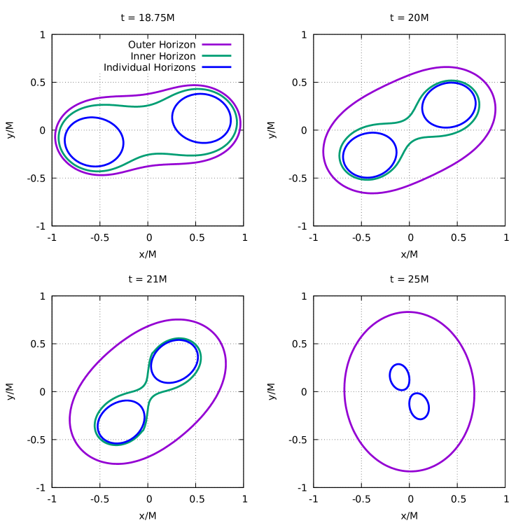
The coordinate shapes of the horizons are depicted in Figs. 3 and 4. For representing the horizon in plots, it is convenient to choose sections of the horizon. Given the presence of reflection symmetry ($z\rightarrow-z$), we shall use the equatorial plane. The first set of plots, Fig. 3, show the shapes of the horizons on the equatorial plane at particular times starting just after the formation of the common horizons, and ending just a short duration before we lose track of the individual horizons. We see that the outer horizon becomes successively more symmetric while the inner horizon becomes highly asymmetric which makes it difficult for the apparent horizon tracker to locate it beyond $t\approx 21M$.

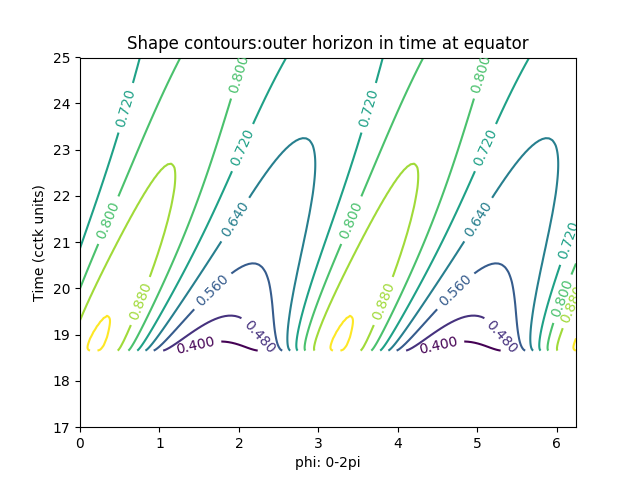
Fig. 4 shows the outer horizon in more detail. This is a somewhat unusual way of depicting the evolution but allows us to avoid showing a large number of two-dimensional plots. We focus again on the equatorial plane on which we have polar coordinates $(r,\phi)$ so that the shape of the horizon can be represented as a radial function $r(\phi)$. To account for the time evolution we will have a sequence of functions $r(\phi;t)$. If the horizon were exactly circular, then $r$ would be constant, but in general it will vary between maximum and minimum values $r_{max}$ and $r_{min}$ respectively. We can then choose a discrete set of values between these extremes and mark, at each value of $t$, the values of $\phi_{i}$ where the values $r_{i}$ are attained. Continuing this at different values of $t$, we obtain the contour plot in the $(\phi,t)$ plane shown in Fig. 4 for the outer common horizon. The fact that at smaller values of $t$, we have more allowed values of $r$ means that the horizon has more irregularities which die away at later times. For example, at $t\approx 19M$, the values of $r$ range between about $0.4$ and $0.96$ while at $t\approx 24M$ the range is only between 0.72 and 0.80. This does give a useful indication of the horizon shape but it is of course coordinate dependent. We shall soon use more coordinate independent geometric multipole moments to quantify how the outer horizon loses its irregularities at later times.

Figure 3: The shape of the inner and outer common horizons, and the two individual horizons on the equatorial plane at four selected times: $t/M=18.75,20,21,25$. The first ($t=18.75M$) is shortly after the common horizon is formed and the third ($t=21M$) is shortly before we lose track of the common inner horizon. In the last panel ($t=25M$), we are unable to locate the common inner horizon and thus only the outer and individual horizons are shown; we lose track of the individual horizons soon after this time. In particular, note that at $t=21M$, portions of the common inner horizon are almost tangential to the y-axis indicating that the inner horizon is close to violating the property of being star shaped. Note also that the inner horizons are rapidly decreasing in size in the coordinate system used in the simulation which causes the horizon finder to lose track of them. This is a gauge effect and the area of these horizons shows no such effect. Different gauge conditions can be used which would make it easier to locate the individual horizons.

Figure 4: The shape of the outer common horizon on the equatorial plane as a function of time. See text for explanation.

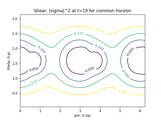
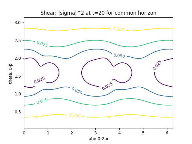
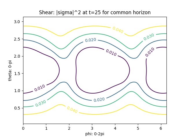
The area increase gives us an overall picture of the growth of the horizon. We can get a detailed picture by looking at the angular distribution of the flux through the common outer horizon. We shall leave a full study of the flux defined in Eq. (5) to a future study and instead just look at the first term in that definition, namely the square of the shear. This term dominates as the horizon gets closer to equilibrium Booth and Fairhurst (2004, 2007). However, the null normals defined in Eq. (2) are not suitable for studying the approach to equilibrium because as the horizon reaches equilibrium and becomes null, $\ell^{a}$ diverges and $n_{a}$ vanishes. There is a more suitable set of null normals used in the simulation. Consider a particular Cauchy surface $\Sigma$ containing a MOTS $\mathcal{S}$. Let $R^{a}$ be the unit spacelike normal to $\mathcal{S}$ on $\Sigma$, and let $T^{a}$ be the unit timelike normal to $\Sigma$. We define the null normals

$$\bar{\ell}^{a}=\frac{1}{\sqrt{2}}(T^{a}+R^{a})\,,\quad\bar{n}^{a}=\frac{1}{\sqrt{2}}(T^{a}-R^{a})\,.$$ (12)

These null normals remain finite throughout the evolution. There must then be a function $b$ such that

$$\bar{\ell}^{a}=b\ell^{a}\,,\quad\bar{n}^{a}=b^{-1}n^{a}\,,$$ (13)

and $b\rightarrow 0$ as the horizon approaches equilibrium. The shear of $\bar{\ell}^{a}$ scales with $b$: $\bar{\sigma}_{ab}=b\sigma_{ab}$.

The modulus of the shear $|\bar{\sigma}|^{2}:=\bar{\sigma}_{ab}\bar{\sigma}^{ab}$ on the horizon at three times, $t/M=19,20,25$, is shown in Fig. 5 as a function of $(\theta,\phi)$. As expected, $|\bar{\sigma}|^{2}$ decreases with time and moreover, at each time, the flux is largest through the poles at $\theta=0,\pi$. We also see that the horizon shape as shown in Fig. 4 has an apparent rotation (see, for example the slope of, say, the $r=0.720$ contour). This is also clear in the apparent rotation of the horizons between the panels of Fig. 3. On the other hand, the contour plots of $|\bar{\sigma}|^{2}$ in Fig. 5 show no such rotation. We will discuss further properties of the flux below.

Figure 5: The shear at the horizon at $t=19,20,25$.

Other interesting quantities to look at are the expansion of the in-going null normal, $\Theta_{(n)}$ to the outer common horizon, and the signatures of the various horizons. The outer common horizon is, as expected, spacelike. The inner horizon becomes partially timelike soon after it is formed and later completely timelike. The individual horizons are null as far as we can tell numerically. Turning now to the in-going expansion, recall from Sec. II.1 that $\Theta_{(n)}<0$ is an ingredient of the definition of a dynamical horizon, and it is used to show that the area of decreases outwards. As expected, the average of $\Theta_{(n)}$ over a MOTS $\mathcal{S}$, defined as

$$\left<\Theta_{(n)}\right>_{\mathcal{S}}:=\frac{1}{A_{\mathcal{S}}}\int_{\mathcal{S}}\Theta_{(n)}\widetilde{\epsilon}\,,$$ (14)

is always negative. However, this is not true point-wise. In fact, it turns out that $\Theta_{(n)}$ is completely negative only at times later than about $\sim 31M$. Thus, strictly speaking, the world tube of MOTSs before this time is not a dynamical horizon. The essential ingredients of the formalism such as the flux laws, multipole moments etc. remain valid. We also point out that the definition of isolated horizons do not involve any condition on $\Theta_{(n)}$ and there are several well known examples where it is not negative everywhere (see e.g. Fairhurst and Krishnan (2001); Geroch and Hartle (1982)). These solutions model situations where a black hole is surrounded by rings of matter which distort the horizon. If the binary black hole coalescence were to occur in the presence of such external matter fields, one would expect portions of the common horizon to have positive $\Theta_{(n)}$ all the way through the merger right through to the final equilibrium state.

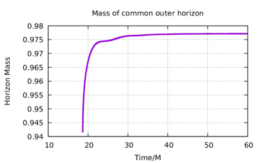
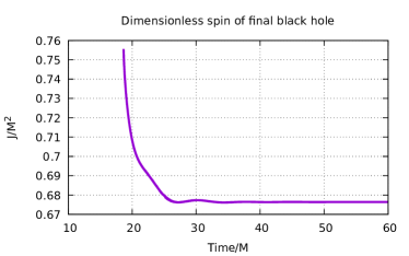
Turning now to the physical properties of the horizon, note that the individual horizons are non-spinning, so their masses are just the irreducible masses, i.e. $\sqrt{A/16\pi}$ which is completely determined by the area. Thus, for angular momentum and mass, only the common horizon is of interest. These are shown in Fig. 6 for the common outer horizon. Just like the area, the mass increases monotonically and reaches an asymptotic value (there is thus no extraction of energy from the black hole, or superradiance). The asymptotic value of the mass is $M_{\infty}\sim 0.977$. The value of the mass at the moment when the common horizon is formed is $\sim 0.941M$ and thus the total increase in the mass of the common- outer horizon is $\Delta M\sim 0.036M$. Similarly, the area of the common horizon increases from $\sim 36.867M^{2}$ to $\sim 41.671M^{2}$, an increase of $\Delta A\sim 4.804M^{2}$. We choose to represent the angular momentum $J$ in terms of the dimensionless quantity $\chi(t)=J(t)/M^{2}(t)$. It can be shown that $\chi$ must always be less than unity Jaramillo et al. (2011b). It is seen to decrease with time, eventually reaching an asymptotic value $\chi\approx 0.68$. This asymptotic value is consistent with the values found already by the earliest successful binary black hole simulations Pretorius (2005); Campanelli et al. (2006); Baker et al. (2006). For later use, we note that the real and imaginary parts of the angular frequency of the $n=0,\ell=m=2$ quasi-normal mode for a Kerr black hole with this dimensionless spin are $M\omega^{(0,2,2)}\approx 0.375-0.089i$.

Figure 6: The angular momentum and mass of the final black hole. The first figure shows the mass $M(t)$ of the common outer horizon as a function of time $t$. The second shows the dimensionless spin, i.e. $J(t)/M(t)^{2}$ with $J$ being the angular momentum.

IV Approach to equilibrium

We have already seen how the area, fluxes, mass and spin of the common horizon evolve and this gives a qualitative picture of the approach to equilibrium. To make this more quantitative, we now turn to the mass and spin multipole moments of the horizon. This was considered previously, using somewhat different notions of multipole moments, by Owen Owen (2009). Instead of using an axial vector as done here, Owen (2009) used eigenfunctions of suitable self-adjoint operators on the horizons.

We start by plotting the moments $M_{n}$ and $J_{n}$ as functions of time for the common outer horizon. Fig. 7 shows the time variation of the mass moments $M_{2,4,6,8}$ and the spin moments $J_{3,5,7}$. Note that the odd-mass and even-spin moments vanish due to reflection symmetry.

Figure 7: The mass and spin moments for the common outer horizon. The inset for both plots is a zoomed version of the bigger plot showing better the time variation of the moments.

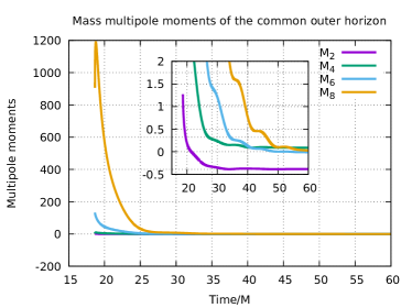
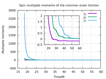
The first immediate observation about the multipole moments is that they decay very rapidly to their asymptotic values. The asymptotic values of the multipole moments are expected to be the ones of a Kerr black hole with mass and angular momentum given by $M_{0}$ and $J_{1}$ respectively. It is clear from Fig. 7 that for most of the multipole moments there is no difficulty in identifying the asymptotic value of the multipole moments. The only exceptions to this are, as shall be clearer on a closer look, $M_{8}$ and $J_{7}$ which are harder to compute numerically because the higher moments require higher angular resolution.

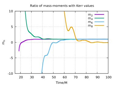
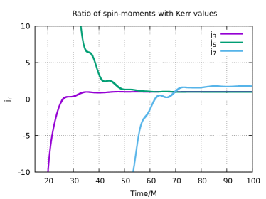
It is instructive to compare the values of the higher multipole moments at each time to the values a Kerr black hole would have with the instantaneous values of mass and angular momentum at that time. It is important to emphasize that these multipoles are different from the Geroch-Hansen multipole moments defined at spatial infinity. This has been considered in Ashtekar et al. (2005) where the differences between these source multipoles and the field moments are calculated. For convenience we give in the Appendix expressions for these multipole moments in terms of the Kerr parameters $M$ and $a$. At each time step $t$, given that we have the mass $M_{\mathcal{S}}(t)$ and angular momentum $J_{\mathcal{S}}(t)$, from the expressions in the appendix, we can calculate $M_{n}^{\textrm{K}err}(t)$ and $J_{n}^{\textrm{K}err}(t)$. We define the ratios

$$m_{n}=\frac{M_{n}(t)}{M_{n}^{\textrm{K}err}(t)}\,,\qquad j_{n}=\frac{J_{n}(t)}{J_{n}^{\textrm{K}err}(t)}\,.$$ (15)

Fig. 8 shows the behavior of these ratios with time. Most moments clearly approach their Kerr values at late times. The exceptions to this are $J_{7}$ and $M_{8}$ which indicates the higher numerical errors in calculating the multipole moments beyond $J_{7}$ and $M_{8}$.

Figure 8: The behavior of the ratios of the mass and spin moments to the corresponding Kerr moments at each instant of the simulation.

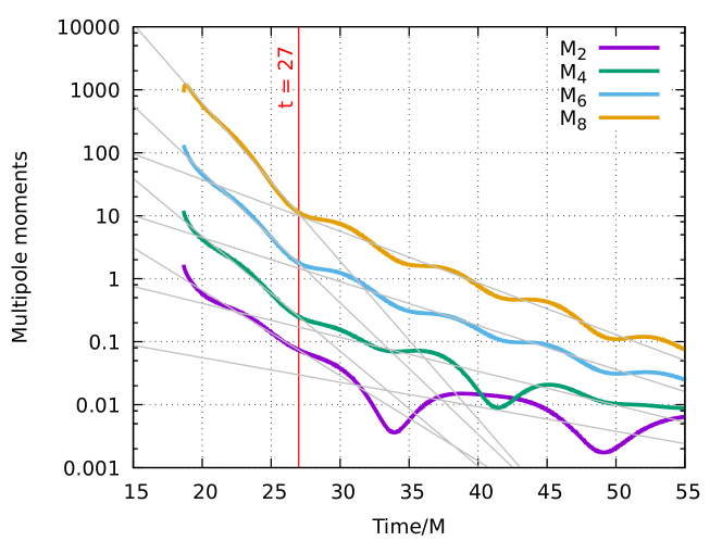
Now we turn to the rate at which the multipole moments decay to their asymptotic values. In the linearized theory, the rate at which perturbations die away is of great physical interest. This was first studied by Price Price (1972). See e.g. Dafermos et al. (2016) for more recent results which proves the linear stability of Schwarzschild black holes. The general issue of the non-linear stability of Kerr black holes is an open question theoretically speaking. Numerical simulations offer the possibility of a better heuristic understanding, and in particular we would like to investigate whether there are any universalities in the approach to equilibrium.

It might seem at first glance that the decay is exponential. Indeed, one could assume a model of the form

$$f(t)=f_{\infty}+Ae^{-\alpha(t-t_{0})}\,,$$ (16)

where $f(t)$ could refer to any of $M_{2,4,6,8}$ or $J_{3,5,7}$, $t_{0}$ is the time at which the common horizon is formed $t_{0}=18.656M$, and $f_{\infty}$ is the asymptotic value of $f$ for large $t$, in this case at $t=100M$. The parameters $A$ and $\alpha$ could be obtained by fitting the model to the numerically computed data.

A closer look reveals that this is in fact not entirely correct. To do this, we plot the decay of the multipoles on a logarithmic scale as shown in Fig. 9 (the multipole moments have been appropriately shifted to make them positive at all times, but still small at late times). Exponential decay would appear as a straight line while Fig. 9 shows different behavior at early and late times separated at $t\approx 27M$, approximately $10M$ after the common horizon first forms. Thus, we fit the multipoles for times $t<27M$ with an exponential decay model using a simple least squares fitting procedure (we fit the logarithm of the moments as a linear function of time), and obtain the values of the decay rates $\alpha$; the results are given in the second column of Tab. 3.

Table 3: Best fit values of the exponent $\alpha$ of Eq. 16 for $M_{2,4,6,8}$ and $J_{3,5,7}$ at early ($t<27M$) and late ($t>27M$) times.

Multipole	$\alpha^{(t<27M)}$	$\alpha^{(t>27M)}$
$M_{2}$	0.31	0.09
$M_{4}$	0.42	0.12
$M_{6}$	0.48	0.16
$M_{8}$	0.58	0.19
$J_{3}$	0.43	0.16
$J_{5}$	0.51	0.17
$J_{7}$	0.64	0.18

(a) Mass multipoles

(b) Spin multipoles

Figure 9: Logarithmic plot of the mass and spin multipoles. A change in the slope is clearly identifiable around the time $27M$. This time corresponds to a time approximately $10M$ after the merger and delineates a substantial change in the behavior of the horizon. The change is most clearly visible in the higher moments but also occurs in $M_{2}$ and $J_{3}$. The figure also shows the best fit straight lines to the portion of the plots before and after $t=27M$ (grey lines).

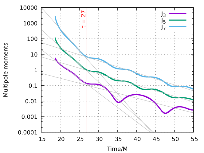
We now turn to the late time behavior of the multipole moments for $t>27M$. Price’s law in the linearized context suggests a power-law fall-off at large times once the exponential part has become negligible. Much more likely, in the regime that we are considering, the moments are linear combinations of exponentially damped functions. To illustrate the differences from the results of the second column of Tab. 3, we continue to use the exponential decay model of Eq. 16. We assume that the moments fall-off as $e^{-\alpha t}$ within the the range $27<t/M<55$ with the upper value being chosen arbitrarily (the values do not change significantly when this is varied). The best fit values of $\alpha$ (again using a least-squares fit) are shown in the third column of Tab. 3.

In addition to these decay terms, the oscillation frequencies of the multipole moments can be determined for $M_{4,6,8}$ and $J_{5,7}$. The angular frequency can simply be determined by calculating the average separation between neighboring peaks in $M_{n}(t)$ and $J_{n}(t)$ after the exponential trends have been removed. This yields a value $M\omega\approx 0.76$ which is roughly twice the dominant quasi-normal mode frequency. The steep fall-off of the multipoles noticeably ends around $t\sim 27M$, roughly $t\approx 10M$ after the common horizon forms. This provides additional support, from a very different viewpoint, with the proposed transition time of $\approx 10M$ from the merger to the ringdown (after the peak of the luminosity) found by Kamaretsos et al. (2012). Caveats to this conclusion are discussed in Sec. VI.

V Cross-correlations between the horizon and the waveform

In the previous sections we have studied the behavior of the various horizons which appear in the process of a binary black hole coalescence. In particular, we have looked at the growth of the individual horizons and the approach of the common-outer horizon to a final Kerr state. Can any of this information be useful for understanding observations of gravitational radiation in the wavezone? Clearly, all of these horizons are hidden behind the event horizon and thus cannot causally affect any observations outside the event horizon. There can however be correlations between fields in the wavezone and the horizon.

The intuitive idea of the cross-correlation idea introduced by Jaramillo et al. is illustrated in Fig. 10. The figure shows a portion of spacetime at late times and shows a source which generically could be due to matter fields or non-linear higher order contributions due to the gravitational field. The source will produce gravitational radiation which can be decomposed into in- and out-going modes which result respectively in-going flux through the horizon and outgoing radiation observed at null infinity, or at large distances from the black hole. The horizon here could be either the event horizon, or more conveniently, a dynamical horizon which asymptotes to the event horizon at future time-like infinity. It is clear that any events at the event or dynamical horizon cannot causally affect observations near null-infinity. However, given that both are the result of time evolution of a given initial data set, there could well be correlations between them.

Figure 10: A spacetime diagram demonstrating cross-correlations between the horizon and null infinity. Future null infinity is $\mathcal{I}^{+}$ where the gravitational waveform is extracted. The event horizon is $\mathcal{E}$, and the dynamical horizon is the spacelike surface $\mathcal{H}$. Future timelike infinity is $i^{0}$ where $\mathcal{E}$, $\mathcal{H}$, $\mathcal{I}^{+}$, and the singularity (the bold dashed horizontal line) all meet. Cauchy surfaces used in the numerical simulation are represented by dashed lines. The common outer horizon is formed at time $t_{0}$ when the Cauchy surface just touches $\mathcal{H}$ in this figure. At later times, the intersection of $\mathcal{H}$ with the Cauchy surfaces yield the outer and inner marginally trapped surfaces $\mathcal{S}_{t}^{outer}$ and $\mathcal{S}_{t}^{inner}$ respectively. The common source is the shaded region which is conjectured to lead to correlations between the horizon (either the event horizon or preferably the dynamical horizon). In this picture, if the formation of the common horizon is to be correlated with the maximum of the outgoing energy flux at $\mathcal{I}^{+}$, the common source for this must be at some earlier time which can causally affect both fields at $\mathcal{H}$ and $\mathcal{I}^{+}$.

Analogous to our earlier analysis at the horizon, we now turn our attention to the wavezone. Due to their practical importance, gravitational waveforms have been extensively studied in the literature. Regarding the approach of the remnant black hole to equilibrium, it is found by Kamaretsos et al. Kamaretsos et al. (2012) that the gravitational waveform may be considered to be in the ringdown phase after a duration $\sim 10M$ following the merger (defined as the peak of the luminosity); see also Thrane et al. (2017) on potential difficulties in ringdown parameter estimation. It is interesting that Fig. 9 also indicates a time of  10M after the formation of the common horizon when the behavior of the horizon multipole moments changes. Whether this is a mere coincidence or if there is a deeper reason is not clear at present. Even if correlations are shown to exist, we have to deal with the different gauge and coordinate conditions employed at the horizon and in the wave-zone and it is far from clear how this should be done.

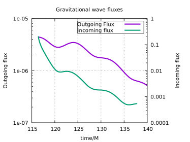
We discuss now additional evidence which lends support to the existence of such correlations. As mentioned in the previous paragraph, Kamaretsos et al. (2012) uses the peak luminosity as the reference time for the merger. The analog of the luminosity is precisely the in-going flux through the dynamical horizon discussed earlier and this is maximum at the moment the common horizon is formed, consistent with the maximum area growth at the time shown in Fig. 1. As also suggested in Jaramillo et al. (2012a, b, 2011a), we choose then to compare the shear $|\bar{\sigma}|^{2}$ at the common horizon integrated over the horizon, with the luminosity of the $\ell=m=2$ mode of $\Psi_{4}$. The luminosity of the outgoing radiation is determined by the News function:

$$\mathcal{N}^{(\ell,m)}(u)=\int_{-\infty}^{u}\Psi_{4}^{(\ell,m)}(u)\,du\,.$$ (17)

Here we have decomposed the waveform $\Psi_{4}$ into spin weighted spherical harmonics and $\Psi_{4}^{(\ell,m)}$ is the corresponding mode coefficient as a function of the retarded time $u=t-r$ (appropriate in the wavezone). Since we extract the waveform on surfaces at fixed $r$, we simply take $\Psi_{4}^{(\ell,m)}$ to be a function of $t$ (starting from the earliest time available in the simulation) and compare $|\mathcal{N}^{(2,2)}|^{2}$ with $|\bar{\sigma}|^{2}$, also as a function of $t$. It is worth emphasizing again that even if one believed in the cross-correlation picture, one would not necessarily expect a good correlation between the two functions. They are measured on surfaces at entirely different positions, one inside the event horizon and one in the wavezone far outside. The gauge condition at these two surfaces, and thus the meaning of the time coordinate for the two quantities, do not need to be related with each other in any way. Nevertheless, if the change in the behavior of the multipole moments at $~{}10M$ after the formation of the common horizon is to be related to the $~{}10M$ for the ringdown analysis found by Kamaretsos et al. (2012), the two must be correlated without adjusting for any gauge choices. Let us therefore go ahead and take $|\mathcal{N}^{(\ell,m)}|^{2}(t)$ and $|\bar{\sigma}|^{2}(t)$, shift the time axis for $|\bar{\sigma}|^{2}(t)$ so that the two peaks are aligned. The result is shown in Fig. 11. By looking at the two plots, the reader can convince herself that the peaks and troughs of the two functions are remarkably aligned. This provides further evidence for the validity of the cross-correlation idea. The oscillation frequency of the News function is, as for the horizon multipoles, twice the frequency of the dominant (i.e. $n=0,\ell=m=2$) quasi-normal mode.

Figure 11: The incoming and outgoing fluxes plotted as functions of ‘ time. The time axis for the in-going flux $|\bar{\sigma}|^{2}$ has been shifted so that it is aligned with the peak outgoing luminosity.

Finally we consider the angular dependence of $|\bar{\sigma}|^{2}$ shown previously in Fig. 5. These figures show a clear quadrupolar pattern. To quantify this we would like to decompose the shear $\bar{\sigma}$ in terms of spin-weighted spherical harmonics. In the Newman-Penrose formalism, we use a null tetrad $(\ell,n,m,\bar{m})$, with $\ell,n$ being null vectors satisfying $\ell\cdot n=-1$, $m$ being a complex null vector satisfying $m\cdot\bar{m}=1$, and all other inner products vanishing. Then, the shear defined in Eq. 4 is written as $\sigma=m^{a}m^{b}\nabla_{a}\ell_{b}$. Under a spin-rotation $m\rightarrow e^{i\psi}m$, $\sigma$ transforms as $\sigma\rightarrow e^{2i\psi}\sigma$ and is said to have a spin-weight 2. Thus, we expect to be able to expand it in terms of spherical harmonics ${}_{2}Y^{\ell}_{m}(\theta,\phi)$ of spin weight 2 Goldberg et al. (1967); Gelfand et al. (1963):

$$\bar{\sigma}=\sum_{\ell=2}^{\infty}\sum_{m=-\ell}^{\ell}\bar{\sigma}^{\ell,m}{}_{2}Y^{\ell}_{m}(\theta,\phi)\,.$$ (18)

However, just as for the multipole moments, this decomposition requires a preferred spherical $(\theta,\phi)$ coordinate system and a suitable area element on the horizon to ensure that the different ${}_{s}Y^{\ell}_{m}$ are orthogonal. Moreover, the proof of being able to expand tensors in terms of the spin weighted spherical harmonics relies on the action of the rotation group Gelfand et al. (1963) which is not available for a highly distorted horizon. Again, as for the multipole moments, we shall ignore these issues for the moment and simply take $(\theta,\phi)$ to be the coordinates used on the horizons in the simulation. Doing this shows, as expected, that $\bar{\sigma}$ is dominated by the $\ell=2,m=2$ and $\ell=2,m=-2$ modes with a much smaller contribution from the $\ell=2,m=0$ mode, which decreases with time. As an example, the ratio $|\bar{\sigma}^{2,2}/\bar{\sigma}^{2,0}|$. At $t=19M$ this has the value $\sim 0.55$, decreasing to $\sim 0.38$ at $t=20M$ and $\sim 0.23$ at $t=25M$.

VI Conclusions

The primary goal of this paper is to study the behavior of marginally trapped surfaces in binary black hole mergers. The main tools used in this analysis are the flux formulae and multipole moments. As seen in other simulations previously, marginally trapped surfaces are formed in pairs. Thus, when the common marginally trapped surface is formed, we get an outer and inner common marginally trapped surface when the two black holes get sufficiently close together. This pair of marginally trapped surfaces form a smooth quasi-local horizon whose area increases monotonically outwards. We have tracked, as far as possible, the areas of the individual horizons and the common horizons. Future work with better gauge conditions and higher accuracy might succeed in finding the eventual fate of the individual horizons and the inner horizon. We have calculated the shear and the fluxes through the common horizon, leading to a detailed picture of how the black hole grows and eventually reaches equilibrium.

We have quantitatively studied how the final black hole settles down to equilibrium. In particular, we have evaluated the falloff of the mass and spin multipole moments and we have shown that the final black hole is Kerr, as expected. We have quantified the falloff of the multipole moments and have found that the moments falloff steeply just after merger, but after about a duration of $10M$ after the merger, the falloff rate changes to a lower rate. This fact might be useful in modeling the gravitational wave signal in the merger phase. These might provide useful hints for proving the non-linear stability of Kerr black holes. We have found that for the QC-0 initial configuration and using the multipole moments as defined in this paper, the behavior of the horizon multipole moments under time evolution changes at an epoch $\sim 10M$ after the formation of the common horizon. This is very similar to existing results in the literature regarding the time at which the post-merger gravitational waveform can be considered to be in the ringdown phase. Clearly, this needs to be explored and understood further and better quantified for a wide rage of initial configurations.

The fall-off rates of the multipole moments given in Tab. 3 for $t<27M$ are too steep for them to be related to the $n=0$ quasi-normal modes of the final black hole. If they are at all related to quasi-normal ringing, it must be due to the higher overtones. See e.g. Fig. 1 of Dreyer et al. (2004) where it is clear that the imaginary part of the quasi-normal mode frequency is not greater (in absolute value) than $\sim 0.2$ while the exponents in the second column of Tab. 3 are all greater than $\sim 0.3$. Alternatively, this might be a genuine non-linear effect unearthed by using the multipole moments. However, Bhagwat et al. (2017) using the multipole moments defined in Owen (2009), have found no such transition in the multipoles. There could be several reasons for this. First, note that the multipole moments used here are different from Owen (2009). We have used here the coordinate z-axis (or equivalently, the axial vector $\varphi^{a}=\partial_{\varphi}$) to define the multipole moments. This is almost certainly not accurate just after the merger. The initial steep fall-off might simply be due to this choice producing a non-physical effect (the fluxes and the correlations described in the previous section, which do not depend on axisymmetry, provide some additional evidence for the choice of $~{}10M$ for the transition point independent of the choice of $\varphi^{a}$). The other reason might be related to the initial configuration that we have chosen. It might turn out that both choices of multipole moments are appropriate, but we have just a fraction of an orbit before merger. The additional eccentricity in the initial configuration might be responsible for exciting higher modes in the initial post-merger phase. This would require a simulation with a longer inspiral phase (ideally one tuned to GW150914 or other binary black hole events) to confirm. Eventually, these question can be addressed fully only by a more appropriate choice of multipole moments suited to fully non-symmetric situations as in Ashtekar et al. (2013).

Finally we have correlated the behavior of the horizon to the waveform extracted far away from the black holes. We have found correlations between the in-falling and outgoing fluxes both as functions of time and over angles. These correlations are unexpected especially in light of possible differences in the lapse function at the horizon and at the waveform extraction surface. This lends additional evidence to the results of Jaramillo et al. (2012a, b, 2011a) and might prove to be a useful tool to observationally study the strong field region from gravitational wave detections and in gravitational waveform modeling. An important aspect of this problem is to find the free data that can be specified on a dynamical horizon to solve the Cauchy problem with initial data prescribed on a dynamical horizon. Thus, in order to reconstruct a relevant portion of spacetime depicted in Fig. 10 we would specify data on (portions of) $\mathcal{I}^{+}$ and $\mathcal{H}$. This would be equivalent to specifying data on an initial Cauchy surface in the standard way. For the case when $\mathcal{H}$ is an isolated horizon the problem has been solved Krishnan (2012); Lewandowski (2000); Lewandowski and Pawłowski (2014); Scholtz et al. (2017); Guerlebeck and Scholtz (2018). Furthermore, the free data on a spherically symmetric dynamical horizon has been determined by Bartnik and Isenberg Bartnik and Isenberg (2006). The problem of finding the free data on a general dynamical horizon is yet to be solved.

An important limitation of our approach is the choice of the axial symmetry vector. Given that we are working with a system of equal-mass non-spinning black holes, it is appropriate to take the axial vector on the horizon to be just $\partial_{\varphi}$, i.e. to assume that the spin of the final black hole is aligned with the orbital angular momentum. This will not be a good approximation in more generic situations where we would not expect the horizon to have any symmetries when it is formed. The method presented in Ashtekar et al. (2013), based on finding a suitable class of divergence free vector fields and assuming that the equilibrium state is axisymmetric, deals with this general situation and provides evolution equations for the multipole moments. Forthcoming work will implement these ideas.

Appendix A Expressions for the Kerr multipole moments

We start with the expression for the Kerr metric with mass $M$ and specific angular momentum $a$ in in-going Eddington-Finklestein coordinates $(v,r,\theta,\phi)$:

$$ds^{2}=-\left(1-\frac{2Mr}{\rho^{2}}\right)dv^{2}+2dv\,dr-2a\sin^{2}\theta dr\,d\varphi-\frac{4aMr\sin^{2}\theta}{\rho^{2}}dv\,d\varphi+\rho^{2}d\theta^{2}+\frac{\Sigma^{2}\sin^{2}\theta}{\rho^{2}}\,d\varphi^{2}\,,$$ (19)

where

$$\rho^{2}=r^{2}+a^{2}\cos^{2}\theta\,,\qquad\Delta=r^{2}-2Mr+a^{2}\,,\qquad\Sigma^{2}=(r^{2}+a^{2})\rho^{2}+2a^{2}Mr\sin^{2}\theta\,.$$ (20)

The horizon is located at $\Delta=0$ i.e. at $r=r_{+}$ such that $r_{+}^{2}+a^{2}=2Mr_{+}$. The volume form on a cross-section of the horizon ($r=r_{+}$ and constant $v$) is $\epsilon=(r_{+}^{2}+a^{2})\sin\theta d\theta\wedge d\varphi$. Thus, the area of the horizon is $A=4\pi(r_{+}^{2}+a^{2})$ and the area radius is $R=\sqrt{r_{+}^{2}+a^{2}}$.

The Weyl tensor component $\Psi_{2}$ can be shown to be Chandrasekhar (1985)

$$\Psi_{2}=-\frac{M}{(r-ia\cos\theta)^{3}}\,.$$ (21)

This is in fact the only non-vanishing component of the Weyl tensor for the Kerr spacetime. The multipole moments are integrals of $\Psi_{2}$ which we now define. For mathematically precise proofs we refer to Ashtekar et al. (2005) while here our aim is to derive expressions for the Kerr multipole moments. The analog of $\cos\theta$ on a general axisymmetric horizon is given by an invariant coordinate $\zeta$ defined as

$$\partial_{a}\zeta=R^{-2}\varphi^{b}\epsilon_{ba}\,.$$ (22)

In addition we need $\zeta=+1$ at the north pole and $-1$ at the south pole (the poles being the two points where $\varphi^{a}$ vanishes). It is easy to check that for Kerr we have in fact $\zeta=\cos\theta$. The mass and spin multipoles are then respectively

$$M_{n} = -\frac{MR^{n}}{2\pi}\oint_{S}P_{n}(\zeta)\mathrm{Re}(\Psi_{2})d^{2}S\,,$$ (23)

$$J_{n} = -\frac{R^{n+1}}{4\pi}\oint_{S}P_{n}(\zeta)\mathrm{Im}(\Psi_{2})d^{2}S\,.$$ (24)

For the Kerr horizon, these become, with $x=a/r_{+}$,

$$M_{n} = 8M^{5}R^{n-4}\textrm{Re}\int_{-1}^{1}\frac{P_{n}(\zeta)}{(1-ix\zeta)^{3}}d\zeta\,,$$ (25)

$$J_{n} = 4M^{4}R^{n-3}\textrm{Im}\int_{-1}^{1}\frac{P_{n}(\zeta)}{(1-ix\zeta)^{3}}d\zeta\,.$$ (26)

Here we have used

$$x=\frac{2Ma}{2Mr_{+}}=\frac{2Ma}{r_{+}^{2}+a^{2}}=\frac{8\pi J}{A}\,.$$ (27)

Define $f_{n}(x)$ to be the integral appearing in these expressions. From the properties of the Legendre polynomials and $\Psi_{2}$ under reflections ($\zeta\rightarrow-\zeta$), it follows that $f_{n}$ is automatically real for even $n$ and imaginary for odd $n$. The explicit expressions for the integrals are:

$$f_{2}(x) = \frac{3x+5x^{3}-3(1+x^{2})^{2}\tan^{-1}x}{x^{3}(1+x^{2})^{2}}\,,$$ (28)

$$f_{4}(x) = \frac{15(1+x^{2})^{2}(7+x^{2})\tan^{-1}(x)-81x^{5}-190x^{3}-105x}{2x^{5}(1+x^{2})^{2}}\,,$$ (29)

$$f_{6}(x) = \frac{919x^{7}+5103x^{5}+7665x^{3}+3465x-105(1+x^{2})^{2}(33+18x^{2}+x^{4})\tan^{-1}(x)}{8x^{7}(1+x^{2})^{2}}\,,$$ (30)

$$f_{8}(x) = \frac{315(1+x^{2})^{2}(143+143x^{2}+33x^{4}+x^{6})\tan^{-1}x-3781x^{9}-38232x^{7}-109494x^{5}-120120x^{3}-45045x)}{16x^{9}(1+x^{2})^{2}}\,,$$ (31)

$$f_{3}(x) = \frac{15(1+x^{2})^{2}\tan^{-1}x-15x-25x^{3}-8x^{5}}{x^{4}(1+x^{2})^{2}}\,,$$ (32)

$$f_{5}(x) = \frac{32x^{7}+343x^{5}+630x^{3}+315x-105(1+x^{2})^{2}(3+x^{2})\tan^{-1}(x)}{2x^{6}(1+x^{2})^{2}}\,,$$ (33)

$$f_{7}(x) = \frac{315(1+x^{2})^{2}(143+110x^{2}+15x^{4})\tan^{-1}x-1024x^{9}-22923x^{7}-86499x^{5}-109725x^{3}-45045x}{40x^{8}(1+x^{2})^{2}}\,.$$ (34)

Inserting these in the expressions (25) and (26) yields explicit expressions for $M_{n}$ and $J_{n}$.

References

- Pretorius (2005) Frans Pretorius, “Evolution of Binary Black Hole Spacetimes,” Phys. Rev. Lett. 95, 121101 (2005), arXiv:gr-qc/0507014 .
- Campanelli et al. (2006) Manuela Campanelli, C. O. Lousto, P. Marronetti, and Y. Zlochower, “Accurate evolutions of orbiting black-hole binaries without excision,” Phys. Rev. Lett. 96, 111101 (2006), arXiv:gr-qc/0511048 [gr-qc] .
- Baker et al. (2006) John G. Baker, Joan Centrella, Dae-Il Choi, Michael Koppitz, and James van Meter, “Gravitational wave extraction from an inspiraling configuration of merging black holes,” Phys. Rev. Lett. 96, 111102 (2006), arXiv:gr-qc/0511103 [gr-qc] .
- Baumgarte and Shapiro (2010) T Baumgarte and T Shapiro, Numerical Relativity: Solving Einstein’s Equations on the Computer (Cambridge University Press, 2010).
- Shibata (2016) M Shibata, Numerical Relativity (100 Years of Relativity, Vol 1) (World Scientific, 2016).
- Alcubierre (2008) M Alcubierre, Introduction to 3+1 Numerical Relativity (Oxford University Press, 2008).
- Ashtekar et al. (2004) Abhay Ashtekar, Jonathan Engle, Tomasz Pawłowski, and Chris Van Den Broeck, “Multipole moments of isolated horizons,” Class. Quant. Grav. 21, 2549–2570 (2004), arXiv:gr-qc/0401114 .
- Ashtekar et al. (2013) Abhay Ashtekar, Miguel Campiglia, and Samir Shah, “Dynamical Black Holes: Approach to the Final State,” Phys. Rev. D88, 064045 (2013), arXiv:1306.5697 [gr-qc] .
- Schnetter et al. (2006) Erik Schnetter, Badri Krishnan, and Florian Beyer, “Introduction to dynamical horizons in numerical relativity,” Phys. Rev. D74, 024028 (2006), arXiv:gr-qc/0604015 .
- Ashtekar and Krishnan (2004) Abhay Ashtekar and Badri Krishnan, “Isolated and dynamical horizons and their applications,” Living Rev. Rel. 7, 10 (2004), arXiv:gr-qc/0407042 .
- Booth (2005) Ivan Booth, “Black hole boundaries,” Can. J. Phys. 83, 1073–1099 (2005), arXiv:gr-qc/0508107 .
- Dreyer et al. (2004) Olaf Dreyer, Bernard J. Kelly, Badri Krishnan, Lee Samuel Finn, David Garrison, and Ramon Lopez-Aleman, “Black hole spectroscopy: Testing general relativity through gravitational wave observations,” Class. Quant. Grav. 21, 787–804 (2004), arXiv:gr-qc/0309007 [gr-qc] .
- Abbott et al. (2016) B. P. Abbott et al. (Virgo, LIGO Scientific), “Tests of general relativity with GW150914,” Phys. Rev. Lett. 116, 221101 (2016), arXiv:1602.03841 [gr-qc] .
- Thrane et al. (2017) Eric Thrane, Paul D. Lasky, and Yuri Levin, “Challenges testing the no-hair theorem with gravitational waves,” Phys. Rev. D96, 102004 (2017), arXiv:1706.05152 [gr-qc] .
- Bhagwat et al. (2017) Swetha Bhagwat, Maria Okounkova, Stefan W. Ballmer, Duncan A. Brown, Matthew Giesler, Mark A. Scheel, and Saul A. Teukolsky, “On choosing the start time of binary black hole ringdown,” (2017), arXiv:1711.00926 [gr-qc] .
- Cabero et al. (2017) Miriam Cabero, Collin D. Capano, Ofek Fischer-Birnholtz, Badri Krishnan, Alex B. Nielsen, and Alex H. Nitz, “Observational tests of the black hole area increase law,” (2017), arXiv:1711.09073 [gr-qc] .
- Jaramillo et al. (2012a) Jose Luis Jaramillo, Rodrigo P. Macedo, Philipp Mösta, and Luciano Rezzolla, “Black-hole horizons as probes of black-hole dynamics II: geometrical insights,” Phys. Rev. D85, 084031 (2012a), arXiv:1108.0061 [gr-qc] .
- Jaramillo et al. (2012b) Jose Luis Jaramillo, Rodrigo Panosso Macedo, Philipp Mösta, and Luciano Rezzolla, “Black-hole horizons as probes of black-hole dynamics I: post-merger recoil in head-on collisions,” Phys.Rev. D85, 084030 (2012b), arXiv:1108.0060 [gr-qc] .
- Jaramillo et al. (2011a) J. L. Jaramillo, R. P. Macedo, P. Mösta, and L. Rezzolla, “Towards a cross-correlation approach to strong-field dynamics in Black Hole spacetimes,” Proceedings, Spanish Relativity Meeting : Towards new paradigms. (ERE 2011): Madrid, Spain, August 29-September 2, 2011, AIP Conf. Proc. 1458, 158–173 (2011a), arXiv:1205.3902 [gr-qc] .
- Price and Thorne (1986) R. H. Price and K. S. Thorne, “Membrane Viewpoint on Black Holes: Properties and Evolution of the Stretched Horizon,” Phys. Rev. D33, 915–941 (1986).
- Rezzolla et al. (2010) Luciano Rezzolla, Rodrigo P. Macedo, and Jose Luis Jaramillo, “Understanding the ’anti-kick’ in the merger of binary black holes,” Phys. Rev. Lett. 104, 221101 (2010), arXiv:1003.0873 [gr-qc] .
- Thornburg (2004) Jonathan Thornburg, “A Fast Apparent-Horizon Finder for 3-Dimensional Cartesian Grids in Numerical Relativity,” Class. Quant. Grav. 21, 743–766 (2004), arXiv:gr-qc/0306056 .
- Andersson et al. (2005) Lars Andersson, Marc Mars, and Walter Simon, “Local existence of dynamical and trapping horizons,” Phys.Rev.Lett. 95, 111102 (2005), arXiv:gr-qc/0506013 [gr-qc] .
- Andersson et al. (2009) Lars Andersson, Marc Mars, Jan Metzger, and Walter Simon, “The Time evolution of marginally trapped surfaces,” Class.Quant.Grav. 26, 085018 (2009), arXiv:0811.4721 [gr-qc] .
- Andersson et al. (2008) Lars Andersson, Marc Mars, and Walter Simon, “Stability of marginally outer trapped surfaces and existence of marginally outer trapped tubes,” Adv.Theor.Math.Phys. 12 (2008), arXiv:0704.2889 [gr-qc] .
- Booth et al. (2017) Ivan Booth, Hari K. Kunduri, and Anna O’Grady, “Unstable marginally outer trapped surfaces in static spherically symmetric spacetimes,” Phys. Rev. D96, 024059 (2017), arXiv:1705.03063 [gr-qc] .
- Ashtekar and Krishnan (2002) Abhay Ashtekar and Badri Krishnan, “Dynamical horizons: Energy, angular momentum, fluxes and balance laws,” Phys. Rev. Lett. 89, 261101 (2002), arXiv:gr-qc/0207080 .
- Ashtekar and Krishnan (2003) Abhay Ashtekar and Badri Krishnan, “Dynamical horizons and their properties,” Phys. Rev. D68, 104030 (2003), arXiv:gr-qc/0308033 .
- Ashtekar et al. (2000a) Abhay Ashtekar et al., “Isolated horizons and their applications,” Phys. Rev. Lett. 85, 3564–3567 (2000a), arXiv:gr-qc/0006006 .
- Ashtekar et al. (1999) Abhay Ashtekar, Christopher Beetle, and Stephen Fairhurst, “Isolated horizons: A generalization of black hole mechanics,” Class. Quant. Grav. 16, L1–L7 (1999), arXiv:gr-qc/9812065 .
- Ashtekar et al. (2000b) Abhay Ashtekar, Christopher Beetle, and Stephen Fairhurst, “Mechanics of Isolated Horizons,” Class. Quant. Grav. 17, 253–298 (2000b), arXiv:gr-qc/9907068 .
- Ashtekar et al. (2001) Abhay Ashtekar, Christopher Beetle, and Jerzy Lewandowski, “Mechanics of Rotating Isolated Horizons,” Phys. Rev. D64, 044016 (2001), arXiv:gr-qc/0103026 .
- Ashtekar et al. (2002) Abhay Ashtekar, Christopher Beetle, and Jerzy Lewandowski, “Geometry of Generic Isolated Horizons,” Class. Quant. Grav. 19, 1195–1225 (2002), arXiv:gr-qc/0111067 .
- Krishnan (2014) Badri Krishnan, “Quasi-local black hole horizons,” in Springer Handbook of Spacetime, edited by Abhay Ashtekar and Vesselin Petkov (2014) pp. 527–555, arXiv:1303.4635 [gr-qc] .
- Ben-Dov (2004) Ishai Ben-Dov, “The Penrose inequality and apparent horizons,” Phys. Rev. D70, 124031 (2004), arXiv:gr-qc/0408066 [gr-qc] .
- Booth et al. (2006) Ivan Booth, Lionel Brits, Jose A. Gonzalez, and Chris Van Den Broeck, “Marginally trapped tubes and dynamical horizons,” Class. Quant. Grav. 23, 413–440 (2006), arXiv:gr-qc/0506119 [gr-qc] .
- Chu et al. (2011) Tony Chu, Harald P. Pfeiffer, and Michael I. Cohen, “Horizon dynamics of distorted rotating black holes,” Phys. Rev. D83, 104018 (2011), arXiv:1011.2601 [gr-qc] .
- Hawking and Hartle (1972) S. W. Hawking and J. B. Hartle, “Energy and angular momentum flow into a black hole,” Commun. Math. Phys. 27, 283–290 (1972).
- Booth and Fairhurst (2007) Ivan Booth and Stephen Fairhurst, “Isolated, slowly evolving, and dynamical trapping horizons: geometry and mechanics from surface deformations,” Phys. Rev. D75, 084019 (2007), arXiv:gr-qc/0610032 .
- Cabero and Krishnan (2015) Miriam Cabero and Badri Krishnan, “Tidal deformations of spinning black holes in Bowen-York initial data,” Class. Quant. Grav. 32, 045009 (2015), arXiv:1407.7656 [gr-qc] .
- Gürlebeck (2015) Norman Gürlebeck, “No-hair theorem for Black Holes in Astrophysical Environments,” Phys. Rev. Lett. 114, 151102 (2015), arXiv:1503.03240 [gr-qc] .
- Dreyer et al. (2003) Olaf Dreyer, Badri Krishnan, Deirdre Shoemaker, and Erik Schnetter, “Introduction to Isolated Horizons in Numerical Relativity,” Phys. Rev. D67, 024018 (2003), arXiv:gr-qc/0206008 .
- Ashtekar et al. (2005) Abhay Ashtekar, Jonathan Engle, and Chris Van Den Broeck, “Quantum horizons and black hole entropy: Inclusion of distortion and rotation,” Class. Quant. Grav. 22, L27–L34 (2005), arXiv:gr-qc/0412003 .
- Cook and Whiting (2007) Gregory B. Cook and Bernard F. Whiting, “Approximate Killing Vectors on S**2,” Phys.Rev. D76, 041501 (2007), arXiv:0706.0199 [gr-qc] .
- Owen (2007) Robert Owen, Topics in numerical relativity : the periodic standing-wave approximation, the stability of constraints in free evolution, and the spin of dynamical black holes, Ph.D. thesis, Caltech (2007).
- Lovelace et al. (2008) Geoffrey Lovelace, Robert Owen, Harald P. Pfeiffer, and Tony Chu, “Binary-black-hole initial data with nearly-extremal spins,” Phys. Rev. D78, 084017 (2008), arXiv:0805.4192 [gr-qc] .
- Beetle (2008) Christopher Beetle, “Approximate Killing Fields as an Eigenvalue Problem,” (2008), arXiv:0808.1745 [gr-qc] .
- Beetle and Wilder (2014) Christopher Beetle and Shawn Wilder, “Perturbative stability of the approximate Killing field eigenvalue problem,” Class. Quant. Grav. 31, 075009 (2014), arXiv:1401.0074 [gr-qc] .
- Baker et al. (2002) John G. Baker, Manuela Campanelli, C. O. Lousto, and R. Takahashi, “Modeling gravitational radiation from coalescing binary black holes,” Phys. Rev. D65, 124012 (2002), arXiv:astro-ph/0202469 [astro-ph] .
- Cook (1994) Gregory B. Cook, “Three-dimensional initial data for the collision of two black holes II: Quasi-circular orbits for equal-mass black holes,” Phys. Rev. D50, 5025–5032 (1994), arXiv:gr-qc/9404043 .
- Löffler et al. (2012) Frank Löffler, Joshua Faber, Eloisa Bentivegna, Tanja Bode, Peter Diener, Roland Haas, Ian Hinder, Bruno C. Mundim, Christian D. Ott, Erik Schnetter, Gabrielle Allen, Manuela Campanelli, and Pablo Laguna, “The Einstein Toolkit: A Community Computational Infrastructure for Relativistic Astrophysics,” Class. Quantum Grav. 29, 115001 (2012), arXiv:1111.3344 [gr-qc] .
- (52) EinsteinToolkit, “Einstein Toolkit: Open software for relativistic astrophysics,” .
- Alcubierre et al. (2000) Miguel Alcubierre, Gabrielle Allen, Bernd Brügmann, Thomas Dramlitsch, Jose A. Font, Philippos Papadopoulos, Edward Seidel, Nikolaos Stergioulas, Wai-Mo Suen, and Ryoji Takahashi, “Towards a stable numerical evolution of strongly gravitating systems in general relativity: The Conformal treatments,” Phys. Rev. D62, 044034 (2000), arXiv:gr-qc/0003071 [gr-qc] .
- Alcubierre et al. (2003) Miguel Alcubierre, Bernd Brügmann, Peter Diener, Michael Koppitz, Denis Pollney, Edward Seidel, and Ryoji Takahashi, “Gauge conditions for long term numerical black hole evolutions without excision,” Phys. Rev. D67, 084023 (2003), arXiv:gr-qc/0206072 [gr-qc] .
- Brown et al. (2009) J. David Brown, Peter Diener, Olivier Sarbach, Erik Schnetter, and Manuel Tiglio, “Turduckening black holes: an analytical and computational study,” Phys. Rev. D 79, 044023 (2009), arXiv:0809.3533 [gr-qc] .
- Ansorg et al. (2004) Marcus Ansorg, Bernd Brügmann, and Wolfgang Tichy, “A single-domain spectral method for black hole puncture data,” Phys. Rev. D 70, 064011 (2004), arXiv:gr-qc/0404056 .
- Thornburg (1996) Jonathan Thornburg, “Finding apparent horizons in numerical relativity,” Phys. Rev. D 54, 4899–4918 (1996), arXiv:gr-qc/9508014 .
- Mösta et al. (2015) P. Mösta, L. Andersson, J. Metzger, B. Szilágyi, and J. Winicour, “The Merger of Small and Large Black Holes,” Class. Quant. Grav. 32, 235003 (2015), arXiv:1501.05358 [gr-qc] .
- Booth and Fairhurst (2004) Ivan Booth and Stephen Fairhurst, “The first law for slowly evolving horizons,” Phys. Rev. Lett. 92, 011102 (2004), arXiv:gr-qc/0307087 .
- Fairhurst and Krishnan (2001) Stephen Fairhurst and Badri Krishnan, “Distorted black holes with charge,” Int. J. Mod. Phys. D10, 691–710 (2001), arXiv:gr-qc/0010088 .
- Geroch and Hartle (1982) Robert P. Geroch and J. B. Hartle, “Distorted black holes,” J. Math. Phys. 23, 680 (1982).
- Jaramillo et al. (2011b) Jose Luis Jaramillo, Martin Reiris, and Sergio Dain, “Black hole Area-Angular momentum inequality in non-vacuum spacetimes,” Phys.Rev. D84, 121503 (2011b), arXiv:1106.3743 [gr-qc] .
- Owen (2009) Robert Owen, “The Final Remnant of Binary Black Hole Mergers: Multipolar Analysis,” Phys. Rev. D80, 084012 (2009), arXiv:0907.0280 [gr-qc] .
- Price (1972) Richard H. Price, “Nonspherical Perturbations of Relativistic Gravitational Collapse. II. Integer-Spin, Zero-Rest-Mass Fields,” Phys. Rev. D5, 2439–2454 (1972).
- Dafermos et al. (2016) Mihalis Dafermos, Gustav Holzegel, and Igor Rodnianski, “The linear stability of the Schwarzschild solution to gravitational perturbations,” (2016), arXiv:1601.06467 [gr-qc] .
- Kamaretsos et al. (2012) Ioannis Kamaretsos, Mark Hannam, Sascha Husa, and B. S. Sathyaprakash, “Black-hole hair loss: learning about binary progenitors from ringdown signals,” Phys. Rev. D85, 024018 (2012), arXiv:1107.0854 [gr-qc] .
- Goldberg et al. (1967) J. N. Goldberg, A. J. MacFarlane, E. T. Newman, F. Rohrlich, and E. C. G. Sudarshan, “Spin s spherical harmonics and edth,” J. Math. Phys. 8, 2155 (1967).
- Gelfand et al. (1963) I. M. Gelfand, R. A. Minlos, and Z. Ya. Shapiro, Representations of the rotation and Lorentz groups and their applications (Pergamon Press, New York, 1963).
- Krishnan (2012) Badri Krishnan, “The spacetime in the neighborhood of a general isolated black hole,” Class.Quant.Grav. 29, 205006 (2012), arXiv:1204.4345 [gr-qc] .
- Lewandowski (2000) Jerzy Lewandowski, “Spacetimes Admitting Isolated Horizons,” Class. Quant. Grav. 17, L53–L59 (2000), arXiv:gr-qc/9907058 .
- Lewandowski and Pawłowski (2014) Jerzy Lewandowski and Tomasz Pawłowski, “Neighborhoods of isolated horizons and their stationarity,” Class. Quant. Grav. 31, 175012 (2014), arXiv:1404.7836 [gr-qc] .
- Scholtz et al. (2017) Martin Scholtz, Ales Flandera, and Norman Guerlebeck, “Kerr-Newman black hole in the formalism of isolated horizons,” Phys. Rev. D96, 064024 (2017), arXiv:1708.06383 [gr-qc] .
- Guerlebeck and Scholtz (2018) Norman Guerlebeck and Martin Scholtz, “The Meissner Effect for axially symmetric charged black holes,” (2018), arXiv:1802.05423 [gr-qc] .
- Bartnik and Isenberg (2006) Robert Bartnik and James Isenberg, “Spherically symmetric dynamical horizons,” Class. Quant. Grav. 23, 2559–2570 (2006), arXiv:gr-qc/0512091 .
- Chandrasekhar (1985) S. Chandrasekhar, The mathematical theory of black holes (Oxford Classic Texts in the Physical Sciences, 1985).