Role of quantum fluctuations on spin liquids and ordered phases in the Heisenberg model on the honeycomb lattice

Abstract

Motivated by the rich physics of honeycomb magnetic materials, we obtain the phase diagram and analyze magnetic properties of the spin-$1/2$ and spin-1 $J_{1}-J_{2}-J_{3}$ Heisenberg model on the honeycomb lattice. Based on the SU(2) and SU(3) symmetry representations of the Schwinger boson approach, which treats disordered spin liquids and magnetically ordered phases on an equal footing, we obtain the complete phase diagrams in the $(J_{2},J_{3})$ plane. This is achieved using a fully unrestricted approach which does not assume any pre-defined Ansätze. For $S=1/2$, we find a quantum spin liquid (QSL) stabilized between the Néel, spiral and collinear antiferromagnetic phases in agreement with previous theoretical work. However, by increasing $S$ from $1/2$ to $1$, the QSL is quickly destroyed due to the weakening of quantum fluctuations indicating that the model already behaves as a quasi-classical system. The dynamical structure factors and temperature dependence of the magnetic susceptibility are obtained in order to characterize all phases in the phase diagrams. Moreover, motivated by the relevance of the single-ion anisotropy, $D$, to various $S=1$ honeycomb compounds, we have analyzed the destruction of magnetic order based on a SU(3) representation of the Schwinger bosons. Our analysis provides a unified understanding of the magnetic properties of honeycomb materials realizing the $J_{1}-J_{2}-J_{3}$ Heisenberg model from the strong quantum spin regime at $S=1/2$ to the $S=1$ case. Neutron scattering and magnetic susceptibility experiments can be used to test the destruction of the QSL phase when replacing $S=1/2$ by $S=1$ localized moments in certain honeycomb compounds.

I Introduction

Quantum magnetism on geometrically frustrated lattices is a very active field of research due to the possibility of discovering new states of matter with exotic propertiesbalents . In large spin systems which can be considered as classical, frustration can lead to a large degeneracy of the ground state manifold. In sufficiently low spin systems, the quantum mechanical zero point motion can forbid long range magnetic order and produce a quantum spin liquid state (QSL), a correlated state that breaks no symmetry and possesses topological properties, possibly sustaining fractionalized excitations Anderson1973 ; Fazekas1974 ; Anderson1987 ; Liang1988 ; Sachdev1992 ; Sandvik2005 . Although the triangular lattice was first theoretically proposed by AndersonAnderson1973 as an ideal benchmark to search for the QSL, it was soon found that the $S=1/2$ antiferromagnetic (AF) Heisenberg model on a triangular lattice is magnetically ordered with a 120⁰ arrangement of the spins. However, longer range exchange couplings and/or multiple exchange processes can destabilize the magnetic order of the isotropic triangular model leading to a QSLmerino1999 ; trumper1999 ; merino2014 ; holt2014 . Despite the intense activity, only a small number of triangular materials have been identified as possible candidates for QSL behavior such as the layered organic materialskanoda2016 : $\kappa$-(BEDT-TTF)₂Cu₂(CN)₃, EtMe₃Sb[(Pd(dmit)₂]₂ and the Kagomé latticenorman2017 material Herbertsmithite, ZnCu₃(OH)₅Cl₂. Hence, there is a need to find evidence for QSL behavior in more compounds.

Honeycomb lattice materials have attracted lots of attention in recent years due to their interesting and poorly understood magnetic properties. Inorganic materials such as Na₂Co₂TeO₆ lefrancoise2016 , BaM₂(XO₄)₂ (with X=As) martin2012 , Bi₃Mn₄O₁₂(NO₃) smirnova2009 and In₃Cu₂VO₉ yan2012 are examples of honeycomb lattice antiferromagnets in which the magnitude of the spin varies from $S=1/2$ in BaM₂(XO₄)₂ for M=Co to $S=1$ for M=Ni (with X=As) and to $S=3/2$ in Bi₃Mn₄O₁₂(NO₃). The rather low magnetic ordering temperature of $T_{N}=2$ K in the $S=1/2$ honeycomb antiferromagnet, In₃Cu₂VO₉, and of only 5.35 K in BaCo₂(AsO₄)₂ suggest the possible existence of QSLs in these compounds. Recent inelastic neutron scattering experiments indicate the presence of a QSL in $\alpha$-RuCl₃ banerjee2016 ; banerjee2017 ; do2017 , a material that realizes the Kitaev kitaev2005 quantum spin model on the honeycomb lattice. Single-ion anisotropy of strength $D$ plays an important role in $S=1$ honeycomb magnets such as: asai2016 ; asai2017 Ba₂NiTeO₆, and in Mo₃S₇(dmit)₃ organometallic compounds in which a relatively large $D$ can be induced by spin-orbit coupling.merino2016 ; khosla2017 ; merino2017 ; jacko2017

It is important then to understand theoretically the magnetic properties of interacting localized moments on the frustrated honeycomb lattice as has been previously done on triangular lattices. Although the numerical evidence for a QSL in the half-filled Hubbard model on the honeycomb latticemeng2010 has been questionedsorella2012 , exact diagonalization studies on the $J_{1}-J_{2}$ Heisenberg model with $S=1/2$ have found evidence for short range spin gapped phases for $J_{2}=0.3-0.35$ suggesting the presence of a Resonance Valence Bond (RVB) state.lhuillier2001 The possible existence of a magnetically disordered phase in this parameter regime has been corroborated by more recent numerical work albuquerque2011 ; reuther2011 , including DMRG sheng2013 and series expansions. oitmaa2011 Schwinger boson mean-field theory (SBMFT)auerbach is consistent with these predictions finding a magnetically disordered region between the Néel and spiral phasesLamas . This disordered region consists of a gapped QSL and a valence bond crystal (VBC) phase. In contrast to the $S=1/2$ model, the $S=1$, $J_{1}-J_{2}-J_{3}$ Heisenberg model on the honeycomb lattice remains largely unexplored theoretically in spite of its relevance to several materials as discussed above. DMRG studies suggest the existence of a spin disordered regionsheng2015 arising between the Néel and spiral phases even for this larger $S=1$ case.

Motivated by recent successes of SBMFT in capturing important features of the spin-1/2, $J_{1}-J_{2}$ Heisenberg model on the honeycomb lattice we apply SBMFT to the spin-1/2 and 1 $J_{1}-J_{2}-J_{3}$ Heisenberg model in the full $(J_{2},J_{3})$ parameter range. The SBMFT approach is particularly useful since it can describe ordered and disordered phases on equal footing; the magnetically ordered phases resulting from the condensation of the bosons at particular order wave vectors of the system. We use the SU(2) formulation of the SBMFT in which the relevant Heisenberg model with $S=1/2,1$ is expressed in terms of antiferromagnetic and ferromagnetic bonds which are described through variational parameters gazza1993 ; flint2009 . We also introduce a SU(3) formulationjaime2014 to describe the $S=1$ case which requires three Schwinger bosons instead of the two of the SU(2) formulation. The SU(3) representation is used to adequately deal with the effect of single-ion anisotropy in the Heisenberg model. We have allowed for all possible point group and translational symmetry breakings, keeping as many mean field parameters which avoids biased guesses. Our completely unrestricted solutions to the SBMFT equations has allowed us to obtain a consistent description of the magnetic properties of $S=1/2$ and $S=1$ Heisenberg models in the full $(J_{2},J_{3})$ parameter range.

After obtaining the phase diagram for both the $S=1/2$ and $S=1$ models, we find that a QSL phase is stable over a broad region of the $(J_{2}-J_{3})$ phase diagram extending between the Néel, spiral phase and collinear antiferromagnet (CAF) phases consistent with previous numerical work. Our results agree with previous SBMFT studies restricted to $J_{3}=0$lamas2013 and to the $J_{3}=J_{2}$ linecabra2011 . Within SBMFT we find that the QSL region disappears in the $S=1$ model where a direct transition from the Néel to the spiral phase occurs. This indicates the fragility of the QSL phase as quantum fluctuations are reduced from $S=1/2$ to $S=1$, the latter behaving as cuasi-classical system. We characterize the different phases by computing the dynamical spin structure factor and the magnetic susceptibility in the different phases. Having in mind the $S=1$ materials we explore the effect of the single-ion anisotropy on the Néel order. We find that the Néel is destabilized at a sufficiently large $D>D_{c}$, where a transition to a trivial paramagnet consisting on the tensor product of $S_{z}=0$ states occurs. The critical single-ion anisotropy strength, $D_{c}$, is found to be rapidly suppressed by frustration suggesting a possible route to induce a quantum paramagnetic phase in $S=1$ compounds such as Mo₃S₇(dmit)₃.

In Sec. II we introduce the frustrated $J_{1}-J_{2}-J_{3}$ Heisenberg model on the honeycomb lattice we have studied and the SBMFT approach in the SU(2) representation we have used to solve the model. In Sec. III we obtain the SBMFT phase diagrams of the $S=1/2$ and $S=1$ models comparing them in detail. The temperature dependence of the magnetic susceptibilty is obtained and discussed in Sec. IV whereas in Sec. V we analyze the dynamic structure factor. In Sec. VI single-ion anisotropy effects in the $S=1$ model are analyzed using the SU(3) slave boson representation. We end up with some conclusions in Sec. VII.

II Model and methods

The $J_{1}-J_{2}-J_{3}$ Heisenberg model is written:

$${\cal H} = \sum_{i<j}J_{ij}S_{i}\cdot S_{j}$$

where $\mathbf{S}_{i}$ is the spin operator at site $i$, $J_{ij}$ the coupling constant which is non zero only for first $(J_{1})$, second $(J_{2})$ and third $(J_{3})$ neighbors, as summarized in Fig. 1, together with the basic properties of the honeycomb lattice.

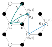
Figure 1: The honeycomb lattice is defined by the translation generator vectors $({\bf e}_{1},{\bf e}_{2})$ and two sublattices $u$ and $v$. The spin-spin exchange couplings up to third neighbors are depicted.

In order to study this Hamiltonian, we consider the Schwinger Boson mean field theory that allows to treat on an equal footing disordered phases such like quantum spin liquids (QSL) and magnetically ordered phases. The idea behind the SBMFT is to express the spin operators in terms of bosons that carry the spin. Usually, a SU(2) representation is considered, namely two bosonic flavors are introduced to describe the spins. This SU(2) representation is not restricted to spins 1/2 though, and the value of the spin $S$ is controlled by a boson constraint that ensures the commutation rule to be preserved under the transformation. Following [auerbach, ; Wang2010, ; Halimeh2016, ], we introduce bosons that mimic the behavior of the spin through the mapping:

$$\mathbf{S}_{i}=\frac{1}{2}b_{i,\alpha}^{+}\mathbf{\tau}_{\alpha,\beta}b_{i,\beta}$$ (1)

where $\mathbf{\tau}$ are the Pauli matrices, $b_{i\sigma}^{+}$ the boson creation operator of spin $\sigma$ on site $i$. As said, in order to preserve the SU(2) commutation rule, the following local constraint has to be fulfilled on each site:

$$b_{i\uparrow}^{+}b_{i\uparrow}+b_{i\downarrow}^{+}b_{i\downarrow} = 2S.$$ (2)

However, it is technically very hard to verify this constraint exactly, thus it will be imposed on average on each site of the lattice by introducing Lagrange multipliers $\mu_{w}$, with $w=u,v$ the sublattice index.

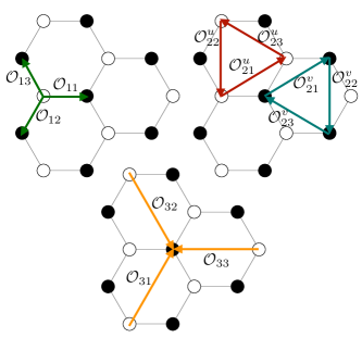
Figure 2: The twelve independent mean field complex parameters ${\cal O}_{id}$ and their clockwise orientation conventions allowing point group symmetry breaking on the lattice. The first subscript $i$ refers to the neighbors (first, second and third), while the second $d$ refers to the three directions. Note that for the second neighbors $i=2$, connected sites are on the same sublattices, we then introduce two sets of mean field parameters labelled with the extra subscript ${\cal O}^{w}$.

One can introduce two SU(2) invariant quantities from which the Hamiltonian could be rewritten flint2009 :

$$\hat{A}_{ij} = \frac{1}{2}\left[b_{i\uparrow}b_{j\downarrow}-b_{i\downarrow}b_{j\uparrow}\right],$$ (3)

$$\hat{B}_{ij} = \frac{1}{2}\left[b_{i\uparrow}^{+}b_{j\uparrow}+b_{i\downarrow}^{+}b_{j\downarrow}\right].$$ (4)

$\hat{A}_{ij}^{+}$ creates a singlet on the oriented bond $(i,j)$ while $\hat{B}_{ij}$ allows for spinon hopping on the same bond. It is clear from these two quantities that the first one is favored in a gapped disordered phase where spins are paired together as singlets, while the second needs an ordered background to allow the spinon for hopping. It can be easily verified that:

$$\mathbf{S}_{i}\cdot\mathbf{S}_{j} = :\hat{B}_{ij}^{+}\hat{B}_{ij}:-\hat{A}_{ij}^{+}\hat{A}_{ij}$$

where $:\hat{O}:$ refers to the normal ordering. This allows for a simple re-expression of the Hamiltonian, and after a mean field decoupling on $\hat{A}$ and $\hat{B}$ operators:

$$\hat{A}_{ij}^{+}\hat{A}_{ij} \to A_{ij}^{*}\hat{A}_{ij}+\hat{A}_{ij}^{+}A_{ij}-A_{ij}^{*}A_{ij}$$ (6)

$$\hat{B}_{ij}^{+}\hat{B}_{ij} \to B_{ij}^{*}\hat{B}_{ij}+\hat{B}_{ij}^{+}B_{ij}-B_{ij}^{*}B_{ij}$$ (7)

the final effective Hamiltonian is only expressed as bilinears of boson operators. In this expression, $A$ and $B$ are complex mean field parameters to be calculated from:

$$A_{ij} = \langle\textrm{gs}|\hat{A}_{ij}|\textrm{gs}\rangle~{}~{},~{}~{}B_{ij}=\langle\textrm{gs}|\hat{B}_{ij}|\textrm{gs}\rangle.$$ (8)

Note that the ground state wave function $|\textrm{gs}\rangle$ is the vacuum of the boson spectrum in this language, namely a state without any Bose condensation. On finite system a finite gap scaling as $\sim 1/\sqrt{n_{c}}$ is always present. This ensures us that the above definitions of $A$ and $B$ are always verified.

Since only exchange couplings up to third neighbors are considered, that we want to preserve the translational invariance of the solutions by allowing for rotational symmetry breaking, we are ending up with 24 inequivalent mean field parameters called ${\cal O}_{id}$, 12 for $A$ and 12 for $B$. The first subscript $i$ refers the neighbor (1, 2 or 3) while the second $d$ to one of the three possible neighbors at distance $i$. This is summarized in Fig.2, as well as the bond orientation we have used.

The final SU(2) Hamiltonian, up to a constant, is expressed as:

$$H = \sum_{i<j}J_{ij}\left[B_{ij}^{*}\hat{B}_{ij}+B_{ij}\hat{B}_{ij}^{+}-A_{ij}^{*}\hat{A}_{ij}-A_{ij}\hat{A}_{ij}^{+}\right]$$ (9)

$$+ \sum_{i}\mu_{i}\left[\sum_{\sigma}b_{i\sigma}^{+}b_{i\sigma}-2S\right]-\langle H\rangle.$$

This mean field Hamiltonian can be block diagonalized by rewriting it in the Fourier space. The unit cell of Fig.1 contains two sites $w=u,v$ and any site $i$ of the lattice can be repaired by the unit cell coordinate ${\bf r}$ and the sub lattice $w$. We then define the Fourier transform of the boson operators as:

$$b_{{\bf{r}},w} = \frac{1}{\sqrt{n_{c}}}\sum_{\bf q}e^{i{\bf q}\cdot{\bf r}}b_{{\bf q},w}$$ (10)

with $n_{c}$ the number of unit cells in the lattice. The mean field Hamiltonian then becomes:

$$H = \sum_{\bf q}\Psi_{\bf q}^{+}M_{\bf q}\Psi_{\bf q}-(2S+1)n_{c}\sum_{w}\mu_{w}-\langle H\rangle$$ (11)

with $\Psi_{\bf q}=(b_{{\bf q}\uparrow}^{u},b_{{\bf q}\uparrow}^{v},b_{-{\bf q}\downarrow}^{u+},b_{-{\bf q}\downarrow}^{v+})^{T}$ a four component Nambu spinor, the 4$\times$4 matrix $M_{q}$ given by

$$M_{\bf q} = \frac{1}{2}\begin{bmatrix}J_{2}(B_{2d}^{u*}\phi_{2d}+B_{2d}^{u}{\phi}^{*}_{2d})+\mu_{u}&J_{1}B_{1d}{\phi}^{*}_{1d}+J_{3}B_{3d}{\phi}^{*}_{3d}&J_{2}A_{2d}^{u*}({\phi}_{2d}-{\phi}^{*}_{2d})&-J_{1}A_{1d}^{*}{\phi}^{*}_{1d}-J_{3}A_{3d}^{*}{\phi}^{*}_{3d}\\ J_{1}B_{1d}^{*}\phi_{1d}+J_{3}B_{3d}^{*}\phi_{3d}&J_{2}(B_{2d}^{v*}\phi_{2d}+B_{2d}^{v}{\phi}^{*}_{2d})+\mu_{v}&J_{1}A_{1d}^{*}\phi_{1d}+J_{3}A_{3d}^{*}\phi_{3d}&J_{2}A_{2d}^{v*}({\phi}_{2d}-{\phi}^{*}_{2d})\\ J_{2}A_{2d}^{u}({\phi}^{*}_{2d}-{\phi}_{2d})&J_{1}A_{1d}{\phi}^{*}_{1d}+J_{3}A_{3d}{\phi}^{*}_{3d}&J_{2}(B_{2d}^{u*}\phi_{2d}^{*}+B_{2d}^{u}{\phi}_{2d})+\mu_{u}&J_{1}B_{1d}^{*}{\phi}^{*}_{1d}+J_{3}B_{3d}^{*}{\phi}^{*}_{3d}\\ -J_{1}A_{1d}\phi_{1d}-J_{3}A_{3d}\phi_{3d}&J_{2}A_{2d}^{v}({\phi}^{*}_{2d}-{\phi}_{2d})&J_{1}B_{1d}{\phi}_{1d}+J_{3}B_{3d}{\phi}_{3d}&J_{2}(B_{2d}^{v*}\phi_{2d}^{*}+B_{2d}^{v}{\phi}_{2d})+\mu_{v}\end{bmatrix}$$

where a summation over repeated indices is assumed, and $\phi_{i,d}({\bf q})=e^{i{\bf q}\cdot{\bf\delta}_{i,d}}$ the phase factor induced between two neighboring sites of distance $\delta_{i,d}$ from i${}^{\text{th}}$ neighbors (1, 2 or 3) and in one of the three directions $d$ as displayed in Fig.2.

Now, we perform a Bogolioubov transformation of the matrix $M_{\bf q}$ which preserves the bosonic communication relations Colpa ; Halimeh2016 , by defining the new bosonic operators $\Gamma_{\bf q}=(\gamma_{{\bf q}\uparrow}^{u},\gamma_{{\bf q}\uparrow}^{v},\gamma_{-{\bf q}\downarrow}^{u+},\gamma_{-{\bf q}\downarrow}^{v+})^{T}$ in such a way that $\Psi_{\bf q}=T_{\bf q}\Gamma_{\bf q}$. The mean field Hamiltonian then takes the diagonal form

$$H = \sum_{\bf q}\Gamma_{\bf q}^{+}\omega_{\bf q}\Gamma_{\bf q}-(2S+1)n_{c}\sum_{w}\mu_{w}-\langle H\rangle$$ (12)

and the matrix $T_{\bf q}$ verifies the following conditions:

$$T_{\bf q}^{+}\tau^{4}T_{\bf q}=\tau^{4},$$ (13)

$$T_{\bf q}^{+}M_{\bf q}T_{\bf q}=\omega_{\bf q},$$ (14)

where

$$\tau^{4} = \begin{bmatrix}{\cal I}_{2}&\\ &-{\cal I}_{2}\end{bmatrix},~{}~{}~{}~{}~{}\omega_{\bf q}=\begin{bmatrix}\epsilon_{+}&\\ &\epsilon_{-}\end{bmatrix}$$ (15)

with ${\cal I}_{2}$ the identity matrix of dimension 2, and $\epsilon_{-}=-\epsilon_{+}$ if time reversal symmetry is preserved Halimeh2016 .

The Bogolioubov transformation matrix $T_{\bf q}$ takes then the specific block form

$$T_{\bf q} = \begin{bmatrix}U_{\bf q}&X_{\bf q}\\ V_{\bf q}&Y_{\bf q}\end{bmatrix}.$$ (16)

Note that an elegant way of finding the Bogolioubov matrix $T_{\bf q}$ is to consider a Choleski decomposition as detailed in [Toth, ]. Now that the mean field Hamiltonian is diagonalized for any ${\bf q}$ point, one can search for a fixed point in the mean field parameter space by minimizing the free energy

$${\cal F}_{\text{MF}} = \sum_{\bf q}\sum_{w}\epsilon_{q,\uparrow}^{w}-(2S+1)n_{c}\sum_{w}\mu_{w}-\langle H\rangle,$$ (17)

with respect to the mean field parameters and the chemical potentials:

$$\frac{\partial{\cal F}_{\text{MF}}}{\partial{\cal O}_{id}}=0,~{}~{}~{}~{}~{}\frac{\partial{\cal F}_{\text{MF}}}{\partial\mu_{w}}=0.$$ (18)

This gives rise to a set of self-consistent equations that are numerically solved. In the same spirit, it is also possible to solve the self consistency by computing at each step the mean field parameters in the gapped ground state as defined in Eq. 8. As pointed out, since we are working on finite systems, an artificial gap is always present even if the ground state at the thermodynamic limit is gapless. This can be used in order to simplify and evaluate Eq. 8.

The advantage of this procedure instead of minimizing the free energy is that no numerical derivative is required. Moreover, the complexness of the mean field parameters is naturally taken into account, which can be of importance if a flux phase is the ground state. Finally, it allows for finding completely unrestricted solutions. However, it is worth emphasizing that using both procedures, we have always obtained same solutions in the present phase diagrams.

The minimization procedure is as follow. First, we start from a given ansätz for the mean field parameters $\{\cal O\}$. Depending the nature of the ground state, this ansätz has to be carefully chosen for helping to a good convergence of the self consistency. This is particularly true in regions of non-commensurate phases as described below.

Plugging the solutions obtained in the large $S$ limit, classical solutions of the Hamiltonian described in the next section, helps us to always find good solutions in any part of the phase diagram.

Then, starting from high value of the chemical potentials and decreasing it, we fulfill the boson constraint of Eq. 2. Once a set of $\{\mu_{w}\}$ is obtained, we diagonalize the mean field Hamiltonian and compute the new set of $\{\cal O\}$ by employing one of the two approaches presented above (derivative of the free energy or explicit computation of the mean field parameters). Then we reconstruct the new Hamiltonian and continue this algorithm until convergence up to an arbitrary tolerance. In our case, the tolerance on the energy is at least $\sim 10^{-12}$ and on the mean field parameters at least $\sim 10^{-9}$.

III Phase diagram

We now obtain and analyze the phase diagrams of the $S=1/2$ and $S=1$ $J_{1}-J_{2}-J_{3}$ Heisenberg model on the frustrated honeycomb lattice. Before discussing the model using the SBMFT approach we briefly revisit the classical phase diagram.

III.1 Classical phase diagram

The classical phase diagram of the $J_{1}-J_{2}-J_{3}$ antiferromagnetic Heisenberg model on a honeycomb lattice has been discussed in the literature lhuillier2001 and we recall here the main results. The classical spin $S$, at unit cell ${\bf r}$ of sublattice $w$ is given by:

$${\bf S}_{rw}\equiv S\cos({\bf Q}\cdot{\bf r}+\phi_{w}){\bf e}_{1}+S\sin({\bf Q}\cdot{\bf r}+\phi_{w}){\bf e}_{2}$$ (19)

where ${\bf Q}$ denotes the magnetic ordering pattern.

We take $\phi_{v}=\phi$ and $\phi_{u}=0$, so $\phi$ is the relative phase between the two sublattices $u$ and $v$. The classical energy per unit cell reads:

$$\frac{E_{\text{class}}}{S^{2}n_{c}} = {J_{1}\over 2}\left[\cos(\phi)+\cos(\phi-Q_{1})+\cos((Q_{1}-Q_{2})+\phi)\right]+J_{2}\left[\cos(Q_{1})+\cos(Q_{2})+\cos(Q_{2}-Q_{1})\right]$$ (20)

$$+ {J_{3}\over 2}\left[\cos(\phi+Q_{1})+\cos(\phi-Q_{1})+\cos(\phi+(Q_{1}-2Q_{2}))\right].$$

The phase diagram, in the $({J_{2}},{J_{3}})$ plane (in unit of $J_{1}$) consistsrastelli1979 ; lhuillier2001 of a Néel ordered phase with ${\bf Q}=(0,0)$ ($\phi=\pi$), a collinear antiferromagnetic phase with ${\bf Q}=(0,\pi)$ ($\phi=\pi$) and a spiral phase with: ${\bf Q}=(Q_{1},Q_{1}/2)$ where $Q_{1}=2\arccos({J_{1}/2-J_{2}\over 2J_{2}-2J_{3}})$ ($\phi=\pi$). The transition lines separating these phases are: (i) $J_{3}/J_{1}={1\over 4}(-1+6{J_{2}\over J_{1}})$ between the Néel and spiral phases. (ii) $J_{2}=0.5$ between the Néel and the CAF phase for $J_{3}/J_{1}>0.5$. (iii) $J_{3}/J_{1}={1\over 4}(1+2{J_{2}\over J_{1}})$ between Néel and spiral phases. They are displayed in Fig. 3 as thin continuous lines to make comparison with the present study. For $J_{3}=0$, an infinitely degenerate collection of spiral states ariseslhuillier2001 ; mulder2010 in the parameter range $J_{2}/J_{1}\in[1/6,1/2]$. The corresponding magnetic ordering vector ${\bf Q}^{*}$, satisfies:

$$\cos(Q^{*}_{1})+\cos(Q^{*}_{2})+\cos(Q^{*}_{1}-Q^{*}_{2})={1\over 8(J_{2}/J_{1})^{2}}-{3\over 2},$$

(21)

with the phase given by the equation:

$$\tan(\phi)={\sin(Q^{*}_{2})+\sin(Q^{*}_{1}+Q^{*}_{2})\over 1+\cos(Q^{*}_{2})+\cos(Q^{*}_{1}+Q^{*}_{2})},$$ (22)

and $Q^{*}_{1}$ and $Q^{*}_{2}$ obtained from Eq. (21). Linear order quantum fluctuations are found to diverge for $J_{2}/J_{1}\gtrsim 0.1$ signaling the destruction of Néel order with no spiral magnetic order. The singular behavior of quantum fluctuations is due to the infinite degeneracy of the planar states found in the classical solution. Classically, only when, $J_{2}\rightarrow\infty$, ($J_{3}=0$) the 120⁰ magnetic order is stabilized since the honeycomb lattice decouples into two isotropic triangular lattices in this limit. However, we show below how quantum fluctuations actually stabilize the 120⁰ order in a region of $(J_{2},J_{3})$ in which it is not expected classically. Nevertheless, the 120⁰ solution is actually part of the spiral states with wave vectors at the corner of the Brillouin zone.

III.2 Quantum fluctuation effects

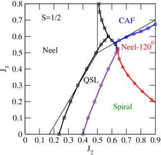
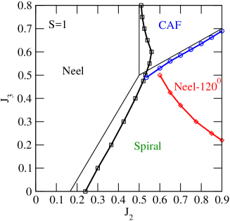
Figure 3: Phase diagram of the $J_{1}-J_{2}-J_{3}$ Heisenberg model on the honeycomb lattice. The $J_{3}$ vs $J_{2}$ phase diagram of the model obtained from SU(2)-SBMFT for $S=1/2$ is compared with the $S=1$ case. There are three types of magnetically ordered phases: Néel antiferromagnet, spiral and collinear antiferromagnet (CAF). The quantum spin liquid (QSL) previously found within SBMFT for $J_{3}=0$ and around $J_{3}=J_{2}/2$ is found in a broad region close to the boundary between the antiferromagnetic and spiral phases only for $S=1/2$. For $S=1$ the QSL disappears and a direct transition from the Néel to the spiral phase occurs. Within the spiral phase, the Néel-120⁰ order is favored by a sufficiently large $J_{3}$. The thin black lines show the classical phase diagram for comparison. We have taken $J_{1}=1$ in the plot.

We now discuss the effect of quantum fluctuations on the classical phase diagram of the model using SU(2)-SBMFT. The $S=1/2$ case has been considered previously in the literature for $J_{3}=0$lamas2013 and $J_{3}=J_{2}$ cabra2011 . Here, we extend these studies to the whole $J_{3}$-$J_{2}$ plane for both $S=1/2$ and $S=1$. It is important to recall here that our mean field solutions are completely unrestricted, in the sense that no particular symmetry is fixed a priori in order to find the most general ones.

In Fig. 3, the SU(2)-SBMFT phase diagrams in the ($J_{2}$,$J_{3}$) plane for $S=1/2$ and $S=1$ are shown. In both cases, there are regions of the phase diagram in which three different classical configurations discussed above are stabilized: the Néel, the spiral and the collinear antiferromagnet. These results are obtainedon clusters up to 36x36 sites.

We recall that the classical transition lines between these phases are shown in Fig. 3 as a guide. As expected, the quantum fluctuations included in the SBMFT also lead to magnetic ordering vectors, ${\bf Q}$, which are different from the classical values and also select a particular configuration from a classically degenerate manifold, the order from disorder effect. For instance, we find the Néel-120⁰ (or close to this order) in a broad region of the phase diagram. Although this spiral order wavevector has the classical form: ${\bf Q}=(Q_{1},Q_{1}/2)$, the magnitude, $Q_{1}$, differs from the classical value in this $(J_{2},J_{3})$ region. i. e. $Q_{1}\neq 2\arccos({J_{1}/2-J_{2}\over 2J_{2}-2J_{3}})$. This can be understood from the quantum fluctuations leading to a magnetically ordered phase different from the classical one as discussed previously.

The $S=1/2$ case. For $J_{3}=0$, quantum fluctuations are found to stabilize the Néel phase above the classical critical ratio $J_{2}/J_{1}\approx 0.2$, recovering previous findings. lamas2013 Spiral order is found at larger ratios, $J_{2}/J_{1}>0.4$, and a gapped quantum spin liquid occurs between the Néel and spiral order for $0.21<J_{2}/J_{1}<0.37$. Quantum fluctuations select a particular wavevector ${\bf Q}$ from the infinite classical manifold defined by Eq. 21 as found previously using linear spin wave theory mulder2010 . Also a staggered valence bond crystal (SVBC) which breaks the rotational $C_{3}$ symmetry of the lattice occurs between the QSL and the spiral phases in a quite narrow parameter range: $0.37<J_{2}/J_{1}<0.4$. We have recovered this phase lamas2013 but due to its very tiny extension, it is almost not visible in our phase diagram and we chose not to display it. The QSL found with SBMFT is qualitatively consistent with DMRG studies in which a non-magnetically ordered phase occurs in the range: $0.22<J_{2}/J_{1}<0.25$. sheng2013 Also a plaquette valence bond crystalwhite2013 ; sheng2013 (PVBC) is found for $0.25<J_{2}/J_{1}<0.35$ between the Néel and a SVBC white2013 which differs from the gapped Z₂ QSL predicted by SU(2)-SBMFT. For non-zero $J_{3}$, the $S=1/2$ SU(2)-SBMFT of Fig. 3 shows how the QSL for $J_{2}=0$ is robust in a broad region located between the Néel, spiral, and CAF phases. This is in good agreement with the QSL found by Cabra et. al. cabra2011 but only along the $J_{3}=J_{2}$ line when $0.41<J/2/J_{1}<0.6$. Our SBMFT phase diagram is also in very good agreement with a recent numerical analysis using exact diagonalization (ED) (see Fig. 2 of Ref. [albuquerque2011, ] for instance), with the phase diagram obtained by pseudo-fermion functional renormalization group (pf-FRG) approach (see Fig. 1 of Ref. [reuther2011, ]) and with the coupled cluster method (see Fig. 2 of Ref. [bishop2012, ]). Series expansionsoitmaa2011 also find a magnetically disordered phase around $J_{3}=J_{2}=0.5J_{1}$ whereas it is inconclusive for other $J_{3}/J_{2}$ ratios.

The $S=1$ case. The SU(2)-SBMFT $(J_{2},J_{3})$ phase diagram for $S=1$ is shown in the lower panel of Fig. 3. The smaller effect of quantum fluctuations compared to $S=1/2$ is evident from the shift of the SBMFT lines towards the classical transition lines, as well as the disappearance of the QSL phase. DMRG studiessheng2015 of the $S=1$ model with $J_{3}=0$ do suggest the existence of a non magnetic disordered phase (possibly a PVBC) in the parameter range $0.27<J_{2}/J_{1}<0.32$ between the Néel and a stripe AF phase, and a magnetically disordered phase is found between $0.25<J_{2}/J_{1}<0.34$ for $S=1$ using the coupled cluster method. bishop2016 In our analysis, we just find a direct transition from the Néel to the spiral phase with no intermediate magnetically disordered phase. It is worth noticing that a careful analysis of the energy of the PVBC solution has been performed, and we have always found that, in the SU(2)-SBMFT description, this solution was slightly above either the Néel and the spiral solutions. Finally, one can see the natural tendency of the boundary lines as $S$ increases to become closer and closer to the classical lines, at the exception of the $120^{o}$ line as already mentioned. As the system is reaching the classical limit, magnetic orders are strengthening until being ideal classical solutions at very large $S$. Anticipating next sections, this explains why the branches observed in the dynamical structure factors for the $S=1/2$ case are blurry in the quantum regime, due to quantum fluctuations, where it should have been very sharp from a linear spin wave theory for example.

IV Magnetic susceptibility

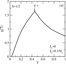
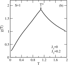
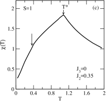
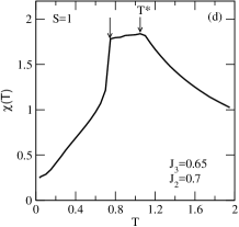
Figure 4: Temperature dependence of magnetic susceptibility for the Heisenberg model on the honeycomb lattice. The temperature dependence of $\chi(T)$ is plotted for the different phases of the model of Fig. 3 obtained at zero temperature $T=0$. In (a) we show the QSL case for $J_{3}=0$ and $J_{2}=0.35J_{1}$ for $S=1/2$, in (b) the Néel ordered phase for $J_{3}=0$, $J_{2}=0.2J_{1}$ for $S=1$, and in (c) the spiral ordered configuration for $J_{2}=0$, $J_{3}=0.35J_{1}$ and for the collinear antiferromagnetic phase: $J_{2}=0.6J_{1}$, $J_{3}=0.7J_{1}$. The vertical arrow in (c) and (d) indicates the temperature at which the relative spin orientation changes. We have taken $J_{1}=1$ in the plot.

The magnetic susceptibility $\chi(T)$ gives information about the difficulty of polarizing the spins in the lattice. We have analyzed the temperature dependence of the susceptibility using SBMFT, by adding Bose-Einstein occupation functions in the free energy of Eq. 17 as well as a weak magnetic field allowing the spin polarization of the Schwinger bosons. All details are provided in appendices A and B. We have explored the finite temperature effects on the different ground states ($T=0$) of the phase diagram of Fig. 3. Since we are dealing with a two-dimensional system with short range interactions, the Mermin-Wagner theorem forbids long range magnetic order at any finite temperature. Hence, if we raise the temperature of a $T=0$ magnetically ordered phase, we should expect the opening of a spin gap and short range correlations. We consider first the case in which the ground state of the system is the disordered QSL phase in the $S=1/2$ model. As temperature is increased, $\chi(T)$ increases indicating the gradual destruction of the RVB spin correlations in the QSL. This behavior occurs until the temperature $T^{*}$ is reached; at this temperature the system crosses over to a paramagnet. In the high temperature regime, the magnetic susceptibility follows a Curie law $\chi(T)\propto 1/T$, as expected for free (non-interacting) localized spins. This high temperature $T>T^{*}$ is encountered in all the parameter ranges explored. If we increase the temperature from $T=0$ for the Néel ordered state, the susceptibility also raises until $T^{*}$ is reached due to the gradual reduction of the spatial extent of the spin correlations with $T$. Above $T^{*}$ again we find the Curie behavior as expected. In the case of the spiral phase, we find that the ground state spiral correlations give way to Néel correlations as temperature is raised above $T\approx 0.4J_{1}<T^{*}\approx 1.1J_{1}$. A similar behavior is also found in the CAF phase. At $T\approx 0.75J_{1}$ a transition from short CAF correlations to Néel correlations occur leading to a plateau in the temperature range $0.75J_{1}<T<1.1J_{1}$ above which the Curie behavior occurs. These thermally induced changes in the spin orientation indicate the proximity of the system to a quantum phase transition to another ground state with a different magnetic order.

We note that $T^{*}$ depends strongly on $S$ being enhanced from $T^{*}=0.45J_{1}$ to $T^{*}=1.1J_{1}$ when $S$ is increased from $S=0.5$ to $S=1$ as expected from the simple mean-field $T^{*}(S)\propto S(S+1)$ scaling relation. This leads to $T^{*}(S=1)=8/3T^{*}(S=0.5)$, consistent with our numerical results. In spite of the similar $T$-dependence of $\chi(T)$ for $T<T^{*}$ there are also crucial differences as $T\rightarrow 0$ depending on whether the ground state of the system is magnetically ordered or not. When the ground state of the system is either the CAF, spiral or Néel ordered phase, $\chi(T)$, goes to a finite value as $T\rightarrow 0$ as shown in Fig. 4 as expected mila2000 . On the other hand, the $T$-dependence of the QSL is very different with the susceptibility dropping exponentially to zeromila2000 , $\chi(T)\propto e^{-\Delta E/k_{B}T}$, due to the spin-gap $\Delta E$. Hence, the SBMFT approach is able to describe the whole $T$-dependenceyu2014 in different ground state configurations of the spins as shown in Fig. 3.

On the basis of our calculations we discuss some recent magnetic susceptibility experiments on Na₂Co₂TeO₆, which features a honeycomb lattice of magnetic Co²⁺ ions with $S=1/2$. A magnetic order transition from a high-temperature Curie paramagnet to a stripe ordered AF (the CAF phase) is observedlefrancoise2016 at $T=T_{N}$. Other features below $T_{N}$ presumably related to a spin reorientation are observed. In order to capture long range magnetic order, a three dimensional model consisting of the $J_{1}-J_{2}-J_{3}$ Heisenberg model describing the honeycomb layers of Co²⁺ atoms coupled through an interlayer, $J_{4}$ has been considered. A classical Monte Carlo evaluation of the model describes the ordering transition at $T_{N}$ but misses the extra features observed in the magnetic susceptibility at $T<T_{N}$. Our present work shows that the temperature dependence of $\chi(T)$ for the $J_{1}-J_{2}-J_{3}$ Heisenberg model including quantum fluctuations (within SBMFT) can be more complex than just the crossover from the Curie paramagnet to the paramagnet with short correlations, containing a richer structure associated with changes in the spin orientations induced by temperature.

V Dynamic structure factor

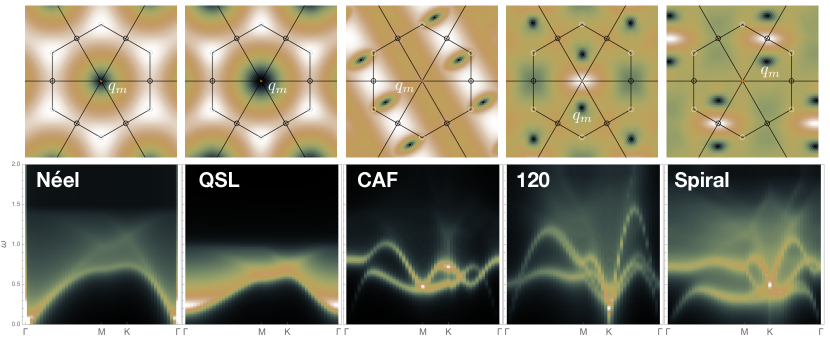
Figure 5: Dispersion relations and dynamic structure factors along the path $\Gamma\to M\to K\to\Gamma$ for the five phases of the S=1/2 model obtained on a $n_{c}=48\times 48$ cluster and discussed in the text. Apart the quantum spin liquid phase, all phases are ordered with a close gap at ${\bf Q}=2{\bf q}_{m}$ where ${\bf q}_{m}$ is the minimum of the dispersion relation.

It is interesting to make connection with neutron experiments and anticipate what would be the signatures of the various phases we have obtained in our model. To this purpose, we have also computed the dynamic spin structure factor defined as

$$S^{\alpha,\beta}({\bf k},\omega) = \frac{1}{n_{c}}\sum_{i,j}e^{i{\bf k}\cdot({\bf r}_{i}-{\bf r}_{j})}\int_{-\infty}^{+\infty}dte^{-i\omega t}\langle\mathbf{S}_{i}^{\alpha}(t)\mathbf{S}_{j}^{\beta}\rangle$$

for the $S=1/2$ case only, because of the redundancy of the phases in the phase diagrams first, but also because we wanted to focus on the case with the more quantum fluctuations. The expression in terms of the block elements of the Bogolioubov matrix $T_{\bf q}$ is detailed in Eq. 30 of [Halimeh2016, ]. In our case, we have derived and diagonalize a sublattice $2\times 2$ matrix, the sum of its eigenvalues being plotted in Fig. 5, together with the dispersion relation of the lowest band $\epsilon_{{\bf q}\uparrow}$. We have considered five representative cases, deep in the domain of each phase, and for a cluster of linear size of 48 unit cells, large enough to focus on the thermodynamic limit properties. In the $(J_{2},J_{3})$ plane and for $J_{1}=1$, the Néel phase is obtained at $(0.1,0)$, the QSL at $(0.3,0)$, the CAF at $(0.8,0.8)$, the spiral at $(0.7,0.1)$ and the 120^o at $(0.8,0.5)$.

Several features appear in these plots. First, while the signature of the excitations in the Néel phase and the quantum spin liquid (QSL) are quite similar because no symmetry is broken, the three other phases present clear distinct features. One has to be careful though, since we plot $S(k,\omega)$ along a specific path connecting high symmetry points of the Brillouin zone, the incommensurate phases has a Bose condensation of magnons (zero mode in the energy) at some ${\bf Q}$ vectors that are not necessarily on this path. As a result, we cannot see the soft modes occurring at these ${\bf Q}$ points, but only the coherent excitations in the neighboring environment. This said, we see that these coherent excitations are quite different for all phases. The most rigid one, the $120$ triangular phase, has the broadest excitations in amplitude, while spectral weights on the two others, the CAF and the Spiral phases, are much smaller than the others. In the QSL, a small gap is observed because of the choice of the parameters $(0.3,0.0)$ corresponding to the very beginning of the gap opening Lamas . Also, we see a very high density of states above the excitation threshold, as expected in a liquid state lacking of substrate for coherent magnetic excitations.

When the gap closes, the system enters the antiferromagnetic Néel state, and one can see a sharpening of the coherent excitations with higher branches. It is worth noticing that a strong continuous background remains present. This is due to quantum fluctuations that lower the net momentum per spin that one would expect for the classical solution.

VI Effect of single-ion anisotropy

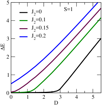
Figure 6: Quantum phase transition from the Néel to the large-$D$ phase in the $J_{1}-J_{2}$ Heisenberg model on the honeycomb lattice with single-ion anisotropy. The dependence of the gap, $\Delta E$, with the single-ion anisotropy, $D$, is shown for different frustration strength. A gap opens up and the Néel order is suppressed around the critical, $D_{c}$, signalling a quantum phase transition to the large-$D$ phase. The plot shows how $D_{c}$ is suppressed by the strength of geometrical frustration, $J_{2}/J_{1}$. We have taken $J_{1}=1$ in the plot.

In real materials, when spins are larger than $1/2$, single-ion anisotropy of strength $D$ can play a crucial role on the nature of the stabilized phases. In particular, when $D$ is very large, and positive $D\gg J_{ij}$, a trivial paramagnetic phase is expected, in competition with the ground state obtained at zero $D$. It is then important, not only from a theoretical perspective, but also for making contact with real experiments, to provide the behavior of all phases upon increasing $D$. Here, we consider the effect of the single-ion anisotropy on the Néel phase of the honeycomb lattice described by the spin-1 $J_{1}-J_{2}$ Heisenberg model on the honeycomb lattice. $J_{3}=0$ already includes the key ingredients between the effect of $D$, magnetic order and magnetic frustration.

Hence we consider the $S=1$ model:

$$H=J_{1}\sum_{\langle ij\rangle}{\bf S}_{i}\cdot{\bf S}_{j}+J_{2}\sum_{\langle\langle ij\rangle\rangle}{\bf S}_{i}\cdot{\bf S}_{j}+D\sum_{i}(S_{i}^{z})^{2}.$$ (24)

In order to properly describe the effect of $D$, the SU(2) description of the SBMFT is no longer efficient, because the SU(3) symmetries are not taken into account, neither the magnetic momenta $0,\pm 1$ expected for a spin one. An elegant way of circumventing this problem is to introduce a SU(3) representation of the spins Wang2017 ; Wang2005 ; pires2015 to deal with this term, as detailed in Appendix C. Hence, we will apply a SU(3)-SBMFT approach to analyze the effect of $D$ on the magnetically ordered phases. For simplicity we consider the above model (in which $J_{2},J_{3}=0$ ) which leads to a Néel phase when $D/J_{1}=0$. As said, in the limit of $D/J_{1}\gg 1$, the ground state is the so-called large-$D$, a trivial paramagnet which consists on the tensor product of $S^{z}_{i}=0$ on all lattice sites. This can be monitored in our mean field SU(3) approach by having a non-zero Bose condensation of bosons carrying the zero magnetic flux.

In Fig. 6 we show the dependence of the gap with $D$ for different $J_{2}$. For $J_{2}=0$, a spin gap opens around $D_{c}\approx 3J_{1}$ signaling the transition from the Néel ordered phase to the large-D phase which consists on the tensor product of $S^{z}_{i}=0$ at all sites. This value is smaller than the $D_{c}=0.72(2z)J_{1}\approx 4.3J_{1}$, where $z=3$ is the coordination of the honeycomb lattice previously obtained in the square lattice. Wang2005 As seen from Fig. 6 as $J_{2}$ is increased, the critical $D_{c}$ is rapidly suppressed so that the quantum paramagnet phase can be stabilized at very small $D$, in agreement with previous analytical results. pires2015 However, caution is in order here since the mean-field treatment of the $b^{\dagger}_{i,0}$ bosons representing the $S^{z}_{i}=0$ states at each lattice site: $\langle b^{\dagger}_{i,0}\rangle=\langle b_{i,0}\rangle=s_{0}$ provides a reliable description of the large-$D$ phase. Hence, we expect a breakdown of the theory when $D\rightarrow 0$. Nevertheless, our analysis does indicate that a large-$D$ phase can be induced at rather small $D$ in the presence of geometrical frustration. We conclude that in a $S=1$ honeycomb material with single-ion anisotropy a quantum phase transition from the Néel ordered state to the quantum paramagnet large-$D$ phase is favored by effectively increasing the frustration of the lattice. These results are relevant to the magnetic properties of the layers of Mo₃S₇(dmit)₃ materials which realize a $S=1$ honeycomb lattice with single-ion anisotropy, $D$, induced by the spin-orbit coupling merino2016 ; merino2017 .

VII Conclusions

In the present work we provide further evidence for the existence of a QSL in a broad region of the phase diagram of the spin-$1/2$, $J_{1}-J_{2}-J_{3}$ Heisenberg model on the honeycomb lattice. This result is consistent with previous theoretical works which have used numerical approaches. Our result is important since, at present, there is no exact method for solving this model and different approximations can, in principle, lead to different results. Also the SBMFT is a much more simple and less computationally costly than the heavy numerical approaches already used. We also find that when the spin is enlarged to $S=1$, the QSL region disappears and the phase diagram closely resembles the classical phase diagram indicating the small effect of quantum fluctuations in this case. Hence, our SBMFT analysis suggests that it is unlikely that a QSL could exist in $S=1$ honeycomb compounds which are described by the $S=1$ $J_{1}-J_{2}-J_{3}$ Heisenberg model.

We have characterized the different ground states by computing the magnetic susceptibility and dynamic structure factor which can be directly compared with experimental observations. At large temperatures the Curie behavior expected for non-interacting localized moments of spin-$S$ is recovered by SBMFT. As temperature is lowered below $T^{*}$ a suppression of $\chi(T)$ signaling the onset of short range spin correlations occurs. While for the Z₂ spin liquid phase found with SBMFT, $\chi(T)\rightarrow 0$, as expected in a spin-gapped state, $\chi(T)\rightarrow const.$ in the magnetically ordered phases. When temperature is increased in the CAF phase, we find a jump in the magnetic susceptibility at $T<T^{*}$ due to a change in the spin orientations induced by temperature. The dynamic structure factor typically displays a sharp magnon-like dispersion arising from the triplet combination of two spinons and a weaker background associated with the particle-hole type excitations in the spinon continuum.

The effect of the single-ion anisotropy term is known to be relevant to $S=1$ honeycomb compounds. For instance, in Ba₂NiTeO₆ the stripe magnetic ordered structure can be described based on a $J_{1}-J_{2}-J_{3}$ honeycomb model with $J_{3}\lesssim 0$, $J_{2}/J_{1}\sim 2$, and a relatively large negative $D=-1.4J_{1}$ contribution which is essential to stabilize the observed stripe order. The presence of $D$ is also crucial to understand the robustness of the stripe phase observed when Ni is changed by Co to form Ba₂CoTeO₆ in spite of the large suppression of the $J_{2}/J_{1}=0.5$ ratio estimated from first principles. The effect of single-ion anisotropy is also relevant to the honeycomb layers of the organometallic compound, Mo₃S₇(dmit)₃. A transition to the large-$D$ phase can be induced for $D>D_{c}$, where $D_{c}$ is strongly suppressed by the frustration of the lattice. Even if this large $D$-limit cannot be reached it would be interesting to analyze the effect of quantum fluctuations on magnetic properties, arising in ordered phases close to the quantum disordered large-D phase.

As stated, our work adds further theoretical support in favor of the existence of a magnetically disordered region in the phase diagram of the $S=1/2$ $J_{1}-J_{2}-J_{3}$ Heisenberg model on the honeycomb lattice. However, the character of such disordered phase is predicted to be different depending on the method used. While the SBMFT used here predicts a gapped Z₂ quantum spin liquid, ED on small clusters as well as variational Monte Carlo approachesferrari2017 find a PVBC. Hence, more theoretical work is needed to unambiguously determine the nature of the quantum paramagnetic phase. It is highly desirable to extend the phase diagram to finite temperatures for a complete comparison with experimental observations and to check the validity of the model for real materials.

Experimental efforts on searching for a QSL should concentrate on $S=1/2$ honeycomb compounds realizing the $J_{1}-J_{2}-J_{3}$ Heisenberg model with $(J_{2},J_{3})$ in the disordered region of Fig. 3. Typically most of quasi-two-dimensional honeycomb materials display long range magnetic order of the Néel, spiral and/or CAF type. Exceptions are the $S=3/2$ Bi₃Mn₄O₁₂(NO₃) which displays no signs of magnetic order down to 0.4 K, In₃Cu₂VO₉ or possibly BaCo₂(AsO₄)₂. The $S=3/2-2$ material, CaMn₂Sb₂, is a Néel magnet which, however, displays coexistent short range magnetic order of different typesmcnally2015 . This unconventional behavior has been interpreted in terms of the proximity of this compound to the spiral phasemazin2013 of the $J_{1}-J_{2}-J_{3}$ classical phase diagram with $J_{3}\approx 0$. Replacing Mn by a lower spin transition metal ion such as Co should enhance quantum fluctuation effects which could turn the Néel state into a QSL state.

Appendix A Finite temperature Schwinger bosons and Bose condensation

In order to derive the self-consistent equations taking into account Bose condensates and thermal fluctuations, one has to write down the Free energy from the diagonalized mean-field Hamiltonian.

The most general mean-field hamiltonian obtained after diagonalization:

$$H = \sum_{{\bf q},w}\epsilon_{{\bf q}\uparrow}^{w}\left[\gamma_{{\bf q}\uparrow w}^{+}\gamma_{{\bf q}\uparrow w}+\gamma_{-{\bf q}\downarrow w}^{+}\gamma_{-{\bf q}\downarrow w}+1\right]$$

$$+ n_{s}K(\left\{{\cal O}\right\},\left\{\mu\right\})$$

with $K(\left\{{\cal O}\right\}$ a function depending on the mean field parameters and the chemical potentials as in Eq. 9. The Bogolioubov bosonic operators $\gamma_{a{\bf q}\uparrow}^{+}$ are of dimension 4, 2 for the sublattice $u$ or $v$, two for the spin flavor and $n_{s}$ is the number of unit cells in the Bravais lattice.

The free energy is defined as:

$${\cal F} = -\frac{1}{\beta}\ln\text{Tr}e^{-\beta H}$$ (25)

where the trace runs over the number of bosons of type $n_{{\bf q}\uparrow}^{w}$ and $n_{-{\bf q}\downarrow}^{w}$. Hence, we have:

$${\cal F} = -\frac{1}{\beta}\ln\text{Tr}e^{-\beta\left[\sum_{{\bf q},w}\epsilon^{w}_{{\bf q}\uparrow}\left(n_{{\bf q}\uparrow}^{w}+n_{-{\bf q}\downarrow}^{w}+1\right)+n_{s}K\right]}$$ (26)

$$= n_{s}K+\sum_{{\bf q},w}\epsilon^{w}_{{\bf q}\uparrow}$$

$$- \frac{1}{\beta}\ln\left[\text{Tr}e^{-\beta\sum_{{\bf q},w}\omega^{w}_{{\bf q}\uparrow}\left(n_{{\bf q}\uparrow}^{w}+n_{-{\bf q}\downarrow}^{w}\right)}\right]$$

$$= n_{s}K+\sum_{{\bf q},w}\epsilon^{w}_{{\bf q}\uparrow}+\frac{2}{\beta}\sum_{{\bf q},w}\ln\left[1-e^{-\beta\epsilon^{w}_{{\bf q}\uparrow}}\right]$$

From the free energy per unit-cell $f={\cal F}/n_{s}$, one can derive the self-consistent (SC) equations at finite temperature and dependent on the Bose-Einstein occupation function $n_{\text{BE}}(\epsilon_{{\bf q}\uparrow})$:

$$\frac{\partial f}{\partial\alpha} = \frac{\partial K}{\partial\alpha}+\frac{1}{n_{s}}\sum_{{\bf q},w}\frac{\partial\epsilon^{w}_{{\bf q}\uparrow}}{\partial\alpha}+\frac{2}{n_{s}\beta}\sum_{{\bf q},w}\frac{\partial\ln\left[1-e^{-\beta\epsilon^{w}_{{\bf q}\uparrow}}\right]}{\partial\alpha}=0$$

where $\alpha$ is one of the mean-field parameter $\left\{{\cal O}\right\}$ and $\left\{{\mu}\right\}$. By noticing that:

$$\frac{\partial\ln\left[1-e^{-\beta\epsilon^{w}_{{\bf q}\uparrow}}\right]}{\partial\alpha} = \beta\frac{\partial\epsilon^{w}_{{\bf q}\uparrow}}{\partial\alpha}n_{\text{BE}}(\epsilon^{w}_{{\bf q}\uparrow}),$$ (28)

one obtain the following SC equations:

$$-\frac{\partial K}{\partial\alpha} = \frac{1}{n_{s}}\sum_{{\bf q},w}\frac{\partial\epsilon^{w}_{{\bf q}\uparrow}}{\partial\alpha}\left[1+2n_{\text{BE}}(\epsilon^{w}_{{\bf q}\uparrow})\right]$$ (29)

Due to Mermin-Wagner, there is no phase transition in 2D systems at finite temperature, thus the dispersion relation is always gapped and the ground state is disordered. At $T=0$ however, bosons can condense and one has to properly take into account Bose condensates in the SC equations. Bose condensates appear as soon as the dispersion relation presents soft modes $\epsilon^{w}_{\xi_{n}^{w}}=0$ for any of the $n_{c}^{w}$ q points $\xi_{n}^{w}$. We have explicitely displayed the sublattice index because in the case of several bands, only certains can have a zero mode energy.

Note that it is also possible to extract from these equations the $T=0$ expression of the SC equations taking into account the presence of Bose condensates. Such condensates usually relate to the fact that a symmetry breaking is obtained precisely at these $\xi_{n}^{w}$. Thus, it is possible to obtain the $T=0$ limit simply by imposing the following condition extracted from the boson density constraint on a sublattice $w$:

$$\nu^{w}_{B} = \frac{1}{n_{s}}\sum_{{\bf q}}\frac{\partial\epsilon^{w}_{{\bf q}\uparrow}}{\partial\mu}n_{\text{BE}}(\epsilon^{w}_{{\bf q}\uparrow})$$ (30)

$$\Rightarrow \frac{1}{n_{s}}\frac{\partial\epsilon^{w}_{{\bf q}\uparrow}}{\partial\mu}n_{\text{BE}}(\epsilon^{w}_{{\bf q}\uparrow})\to\frac{\nu^{w}_{B}}{n_{c}^{w}}\sum_{n=1}^{n_{c}^{w}}\delta(k-\xi_{n}^{w})$$

and thus:

$$n_{\text{BE}}(\epsilon^{w}_{{\bf q}\uparrow})\to\nu^{w}_{B}\frac{n_{s}}{n_{c}^{w}}\frac{1}{\frac{\partial\epsilon^{w}_{{\bf q}\uparrow}}{\partial\mu}}\sum_{n=1}^{n_{c}^{w}}\delta({\bf q}-\xi_{n}^{w}).$$ (31)

Plugging this expression in the general form of the SC equation, we obtain finally:

$$-\frac{\partial K}{\partial\alpha} = \frac{1}{n_{s}}\sum_{{\bf q},w}\frac{\partial\epsilon^{w}_{{\bf q}\uparrow}}{\partial\alpha}+2\sum_{w}\frac{\nu^{w}_{B}}{n_{c}^{w}}\sum_{n=1}^{n_{c}^{w}}\frac{\frac{\partial\epsilon^{w}_{\xi_{n}^{w}}}{\partial\alpha}}{\frac{\partial\epsilon^{w}_{\xi_{n_{s}}}}{\partial\mu}}.$$ (32)

Here, one has to be careful. Indeed, at each $\xi$ point, there are two branches in the dispersion relation that are ordered from the lowest to the highest eigenenergy. Usually, the lowest branch reaches the zero but not the highest, and thus only one type of exists. However, it is not excluded that the two branches reach zero at the same $\xi$ points, hence both condensates should exist. Note that it is unlikely, but it has to be checked, that the two types of condensates appear at different $\xi$ points. Finally, in the case for which only one type of the condensate appears, only this type has to be considered in the previous equation.

Appendix B Effect of a magnetic field

Here we show the extension of the finite temperature SU(2) SBMFT formalism to include a magnetic field. The equations described below are used to compute the $T$-dependence of the magnetic susceptibility, $\chi(T)$, discussed in the paper.

The SBMFT under a uniform magnetic field, $B$, along the $z$-axis reads:

$$H(B)=H-{\mu_{B}B\over 2}\sum_{i}\left(\langle b^{\dagger}_{i\uparrow}b_{i\uparrow}\rangle-\langle b^{\dagger}_{i\downarrow}b_{i\downarrow}\rangle\right),$$ (33)

where $H$ is the SBMFT hamiltonian without the magnetic field introduced in Eq. (9). Since the magnetic field just leads to a different chemical potential for the $\uparrow$ and $\downarrow$ bosons: $\mu_{\sigma}=\mu-2\sigma\mu_{b}B/2$, where $\sigma=\pm{1\over 2}$, we can just replace $\mu$ by $\mu_{\sigma}$ leading to different spinon dispersions: $\epsilon_{{\bf q}\uparrow}^{w}\neq\epsilon_{{\bf q}\downarrow}^{w}$ when $B\neq 0$. Hence, the diagonalized hamiltonian in the presence of the magnetic field, $B$, now reads:

$$H(B) = \sum_{{\bf q},\sigma,w}\epsilon_{{\bf q}\sigma}^{w}\left[\gamma_{{\bf q}\sigma w}^{+}\gamma_{{\bf q}\sigma w}+{1\over 2}\right]+n_{s}K(\left\{{\cal O}\right\},\left\{\mu\right\}).$$

Following the same analysis as in the previous section but using $H(B)$ instead of $H$ we arrive at the following SC equations:

$$-\frac{\partial K}{\partial\alpha} = \frac{1}{n_{s}}\sum_{{\bf q},w}\frac{\partial\sigma\epsilon^{w}_{{\bf q}\sigma}}{\partial\alpha}\left[{1\over 2}+n_{\text{BE}}(\epsilon^{w}_{{\bf q}\sigma})\right],$$ (34)

which recovers the SC equations (29) when $B=0$. By evaluating the uniform magnetization, $m_{B}(T)$, induced by a small field, $B$, and taking $B\rightarrow 0$ we can obtain the temperature dependence of the magnetic susceptibility:

$$\chi(T)=\lim_{B\rightarrow 0}{\partial m_{B}(T)\over\partial B},$$ (35)

where the uniform magnetization reads:

$$m_{B}(T)=\sum_{{\bf q},w}\sigma n_{\text{BE}}(\epsilon^{w}_{{\bf q}\sigma}).$$ (36)

Appendix C SU(3) formulation of the Heisenberg model

Following [Wang2017, ; Wang2005, ], in the SU(3) formulation of the $J_{1}-J_{2}$ Heisenberg model (24) we introduce three Schwinger bosons:

$$|1\rangle = b^{\dagger}_{i,+}|0\rangle$$

$$|0\rangle = b^{\dagger}_{i,0}|0\rangle$$

$$|-1\rangle = b^{\dagger}_{i,-}|0\rangle,$$ (37)

whIch represent the $S^{z}=-1,0,+1$ projection of the $S=1$ at each site. The Schwinger bosons at each site satisfy the constraint:

$$b^{\dagger}_{i,+}b_{i,+}+b^{\dagger}_{i,0}b_{i,0}+b^{\dagger}_{i,-}b_{i,-}=1.$$ (38)

The spin operators can be expressed in terms of the Schwinger bosons as:

$$S^{+}_{i} = \sqrt{2}(b^{\dagger}_{i,0}b_{i,-}+b^{\dagger}_{i,+}b_{i,0})$$

$$S^{-}_{i} = \sqrt{2}(b^{\dagger}_{i,-}b_{i,0}+b^{\dagger}_{i,0}b_{i,+})$$

$$S^{z}_{i} = b^{\dagger}_{i,+}b_{i,+}-b^{\dagger}_{i,-}b_{i,-}.$$ (39)

Introducing these operators and assuming the condensation of the 0-bosons: $\langle b^{\dagger}_{i,0}\rangle=\langle b_{i,0}\rangle=s_{0}$, the hamiltonian reads:

$$H = J_{1}s_{0}^{2}\sum_{\langle ij\rangle}\{(b^{\dagger}_{i,-1}b_{j,-1}+b_{i,-1}b^{\dagger}_{j,-1})$$

$$+ (b^{\dagger}_{i,+1}b_{j,+1}+b_{i,+1}b^{\dagger}_{j,+1})$$

$$+ (b^{\dagger}_{i,+1}b^{\dagger}_{j,-1}+b^{\dagger}_{i,-1}b^{\dagger}_{j,+1})$$

$$+ (b_{i,+1}b_{j,-1}+b_{i,-1}b_{j,+1})\}$$

$$+ J_{1}\sum_{\langle ij\rangle}(b^{\dagger}_{i,+1}b_{i,+1}-b^{\dagger}_{i,-1}b_{i,-1})$$

$$\times (b^{\dagger}_{j,+1}b_{j,+1}-b^{\dagger}_{j,-1}b_{j,-1})$$

$$+ J_{2}s_{0}^{2}\sum_{\langle\langle ij\rangle\rangle}\{(b^{\dagger}_{i,-1}b_{j,-1}+b_{i,-1}b^{\dagger}_{j,-1})$$

$$+ (b^{\dagger}_{i,+1}b_{j,+1}+b_{i,+1}b^{\dagger}_{j,+1})$$

$$+ (b^{\dagger}_{i,+1}b^{\dagger}_{j,-1}+b^{\dagger}_{i,-1}b^{\dagger}_{j,+1})$$

$$+ (b_{i,+1}b_{j,-1}+b_{i,-1}b_{j,+1})\}$$

$$+ J_{2}\sum_{\langle\langle ij\rangle\rangle}(b^{\dagger}_{i,+1}b_{i,+1}-b^{\dagger}_{i,-1}b_{i,-1})$$

$$\times (b^{\dagger}_{j,+1}b_{j,+1}-b^{\dagger}_{j,-1}b_{j,-1})$$

$$+ D\sum_{i}(b^{\dagger}_{i,+1}b_{j,+1}+b^{\dagger}_{i,-1}b_{i,-1})^{2}.$$

We can treat the remaining quartic terms by using a further mean-field decoupling so that:

$$(b^{\dagger}_{i,+1}b_{i,+1}-b^{\dagger}_{i,-1}b_{i,-1})(b^{\dagger}_{j,+1}b_{j,+1}-b^{\dagger}_{j,-1}b_{j,-1}) =$$

$${1\over 2}(1-s_{0}^{2})(b^{\dagger}_{i,+1}b_{i,+1}+b^{\dagger}_{j,+1}b_{j,+1})$$

$$+{1\over 2}(1-s_{0}^{2})(b^{\dagger}_{i,-1}b_{i,-1}+b^{\dagger}_{j,-1}b_{j,-1})$$

$$-p_{\delta}(b_{i,+1}b_{j,-1}+b^{\dagger}_{i,+1}b^{\dagger}_{j,-1}+b_{i,-1}b_{j,+1}+b^{\dagger}_{i,-1}b^{\dagger}_{j,+1})$$

$$-{1\over 2}(1-s_{0}^{2})^{2}+2p_{\delta}^{2},$$

where the real mean-field parameter is: $p_{\delta}=\langle b^{\dagger}_{i,-1}b^{\dagger}_{j,+1}\rangle=\langle b_{i,-1}b_{j,+1}\rangle$, with $\delta=1,2$ for the nearest and next-nearest neighbors, respectively.

Fourier transforming the bosons: $b_{{\bf r},w}={1\over\sqrt{n_{c}}}\sum_{\bf q}e^{i{\bf q}{\bf r}}b_{{\bf q},w}$, where $n_{c}$ is the number of cells ($n_{s}=2n_{c}$) the final mean-field Hamiltonian reads:

$$H=\sum_{\bf q}\Psi^{\dagger}_{\bf q}M_{\bf q}\Psi_{\bf q}-\sum_{\bf q}(M^{33}_{\bf q}+M^{44}_{\bf q})+C,$$

where:

$$M_{\bf q} = \begin{bmatrix}A_{\bf q}&B_{\bf q}\\ B_{\bf q}&A_{\bf q}\end{bmatrix},$$

$$A_{\bf q} = \begin{bmatrix}\tilde{\mu}&J_{1}s_{0}^{2}\gamma_{1{\bf q}}\\ J_{1}s_{0}^{2}\gamma^{*}_{1{\bf q}}&\tilde{\mu}\end{bmatrix},$$

$$B_{\bf q} = \begin{bmatrix}J_{2}(s_{0}^{2}-p_{2})\gamma_{2{\bf q}}&J_{1}(s_{0}^{2}-p_{1})\gamma_{1{\bf q}}\\ J_{1}(s_{0}^{2}-p_{1})\gamma^{*}_{1{\bf q}}&J_{2}(s_{0}^{2}-p_{2})\gamma_{2{\bf q}}\end{bmatrix},$$ (43)

and $\tilde{\mu}=\mu+{3\over 2}(1-s_{0}^{2})(J_{1}+2J_{2})+2J_{2}s_{0}^{2}\gamma_{2{\bf q}}+D.$ The dispersion relations read:

$$\gamma_{1{\bf q}} = 1+e^{i(k_{1}-k_{2})}+e^{-ik_{2}},$$ (44)

$$\gamma_{2{\bf q}} = \cos(k_{1})+\cos(k_{2})+\cos(k_{1}-k_{2}),$$ (45)

and finally:

$$\frac{C}{n_{c}} = 3J_{1}\left[2p_{1}^{2}-{1\over 2}(1-s_{0}^{2})^{2}\right]$$ (46)

$$+ 6J_{2}\left[2p_{2}^{2}-{1\over 2}(1-s_{0}^{2})^{2}\right]+2\mu(s_{0}^{2}-1).$$

Diagonalization of $\sigma_{z}\cdot M_{\bf q}$ leads to the Bogoliubov quasiparticle dispersions as described in the main text. The ground state energy per site can then be expressed in terms of these new Bogoliubov quasiparticles as:

$$e_{0}={E_{0}\over 2n_{c}}=\\ {1\over 2n_{c}}\left[\sum_{{\bf q},\omega}\epsilon^{\omega}_{{\bf q}\uparrow}-\sum_{\bf q}(M^{33}_{\bf q}+M^{44}_{\bf q})+C\right],$$

where $\omega=1,2$ denotes the two quasiparticle dispersions. The SC equations obtained from the minimization of the total energy are:

$$p_{1} = -{1\over 12J_{1}n_{c}}\sum_{{\bf q},\omega}{\partial\epsilon^{\omega}_{{\bf q}\uparrow}\over\partial p_{1}}$$

$$p_{2} = -{1\over 24J_{2}n_{c}}\sum_{{\bf q},\omega}{\partial\epsilon^{\omega}_{{\bf q}\uparrow}\over\partial p_{2}}$$

$$2-s_{0}^{2} = {1\over 2n_{c}}\sum_{{\bf q},\omega}{\partial\epsilon^{\omega}_{{\bf q}\uparrow}\over\partial\mu}$$

$$\mu = -2J_{1}-{7\over 2}J_{2}+{3s_{0}^{2}\over 2}J_{1}+3s_{0}^{2}J_{2}-{1\over 2n_{c}}\sum_{{\bf q},\omega}{\partial\epsilon^{\omega}_{{\bf q}\uparrow}\over\partial s_{0}^{2}}.$$

References

- (1) L. Balents, Nature 464 199 (2010).
- (2) P. .W. Anderson, Mat. Res. Bull 8, 153 (1973).
- (3) P. Fazekas and P. .W. Anderson, Phil. Mag. 30, 423 (1974).
- (4) P. .W. Anderson, Science 235, 1196 (1987).
- (5) S. Liang, B. Douçot and P. .W. Anderson, Phys. Rev. Lett. 61, 365 (1988).
- (6) S. Sachdev, Phys. Rev. B45, 12377 (1992).
- (7) A. W. Sandvik, Phys. Rev. Lett. 95, 207203 (2005).
- (8) J. Merino, R. H. Mckenzie, J. B. Marston, and C. H. Chung, J. Phys.: Condens. Matter 11 2965 (1999).
- (9) A. E. Trumper, Phys. Rev. B 60, 2987 (1999).
- (10) J. Merino, M. Holt, and B. J. Powell, Phys. Rev. B 89, 245112 (2014).
- (11) M. Holt, B. J. Powell, and R. H. McKenzie, Phys. Rev. B 89, 174415 (2014).
- (12) Y. Zhou, K. Kanoda, T.-K Ng, Rev. Mod. Phys. 89 025003 (2017).
- (13) M. Norman, Rev. Mod. Phys. 88, 041002 (2016).
- (14) E. Lefrancoise, et al. Phys. Rev. B 94, 214416 (20016).
- (15) N. Martin, L.-P Regnault, and S. Klimko, Jour. Phys. Conf. Ser. 340 012012 (2012).
- (16) O. Smirnova et. al. J. Am. Chem. Soc. 131, 8313 (2009).
- (17) Y. J. Yan et. al., Phys. Rev. B 85 85102 (2012).
- (18) A. Banerjee, et. al. Nat. Mater. 15, 733 (2016).
- (19) A. Banerjee, et. al., Science 356, 1055 (2017).
- (20) S.-H. Do, et. al., Nat. Phys. 13 1079 (2017).
- (21) A. Kitaev, Ann. of Phys. 321 2 (2005).
- (22) S. Asai,M. Soda, K. Kasatani, T. Ono, M. Avdeev, and T.Masuda, Phys. Rev. B 93, 024412 (2016).
- (23) S. Asai, et. al., arXiv:1708.08717v1.
- (24) J. Merino, A. C. Jacko, A. L. Khosla, and B. J. Powell, Phys. Rev. B 94, 205109 (2016).
- (25) A. L. Khosla, A. C. Jacko, J. Merino, and B. J. Powell, Phys. Rev. B 95, 115109 (2017).
- (26) J. Merino, A. C. Jacko, A. L. Khosla, and B. J. Powell, Phys. Rev. B 96, 205118 (2017).
- (27) A. C. Jacko, A. L. Khosla, J. Merino, and B. J. Powell, Phys. Rev. B 95, 155120 (2017).
- (28) Z. Y. Meng, T. C. Lang, S. Wessel, F. F. Assaad, A. Muramatsu, Nature 464, 847 (2010).
- (29) S. Sorella, Y. Otsuka, S. Yunoki, Scientific Reports 2, 992 (2012).
- (30) J.B. Fouet, P. Sindzingre, and C. Lhuillier, Eur. Phys. J B 20, 241 (2001).
- (31) A. F. Albuquerque, D. Schwandt, B. Hetényi, S. Capponi,M. Mambrini, and A. M. Läuchli, Phys. Rev. B 84, 024406 (2011).
- (32) J. Reuther, D. A. Abanin, and R. Thomale, Phys. Rev. B 84, 014417 (2011).
- (33) S.-S. Gong, D. N. Sheng, O. I. Motrunich, and M. P. A. Fisher, Phys. Rev. B 88, 165138 (2013).
- (34) J. Oitmaa and R. R. P. Singh, Phys. Rev. B 84, 094424 (2011).
- (35) A. Auerbach, Interacting Electrons and Quantum Magnetism, Springer-Verlag (1994).
- (36) H. Zhang and C. A. Lamas, Phys. Rev. B 87, 024415 (2013).
- (37) S.-S. Gong, W. Zhu, and D. N. Sheng, Phys. Rev. B 92, 195110 (2015).
- (38) C. J. Gazza and H. A. Ceccatto, J. Phys: Condens. Matter 5, L135 (1993).
- (39) R. Flint and P. Coleman, Phys. Rev. B 79, 014424 (2009).
- (40) V. Kapf, M. Jaime, and C. D. Batista, Rev. Mod. Phys. 86, 563 (2014).
- (41) H. Zhang, and C. A. Lamas, Phys. Rev. B 87, 024415 (2013).
- (42) D. C. Cabra, C. A. Lamas, and H. D. Rosales, Phys. Rev. B 83, 094506 (2011).
- (43) Fa Wang, Phys. Rev. B82, 024419 (2010).
- (44) J. C. Halimeh and M. Punk, Phys. Rev. B94, 104413 (2016).
- (45) J. H. P. Colpa, Phys. A 93, 327 (1978).
- (46) S. Toth and B. Lake, Journal of Physics: Condens. Matter 27, 166002 (2015).
- (47) E. Rastelli, A. Tassi, and L. Reatto, Physica 97B, 1 (1979).
- (48) A. Mulder, R. Ganesh, L. Capriotti, and A. Paramekanti, Phys. Rev. B 81 , 214419 (2010).
- (49) Z. Zhu, D. A. Huse, and S. R. White, Phys. Rev. Lett. 110, 127205 (2013).
- (50) P. H. Y. Li, R. F. Bishop, D. J. J. Farnell, and C. E. Campbell, Phys. Rev. B 86, 144404 (2012).
- (51) P. H. Y. Li and R. F. Bishop, Phys. Rev. B 93, 214438 (2016).
- (52) F. Mila, Eur. J. Phys. 21 499 (2000).
- (53) X.-L Yu, D.-Yong Liu, P. Li, L.-J Zou, Phys. E 59, 41 (2014).
- (54) Zhentao Wang, Adrian E. Feiguin, Wei Zhu, Oleg A. Starykh, Andrey V. Chubukov, and Cristian D. Batista, Phys. Rev. B96, 184409 (2017).
- (55) H.-T. Wang and Y. Wang, Phys. Rev B 71, 104429 (2005).
- (56) A. S. T. Pires, Phys. B, 479, 130 (2015).
- (57) F. Ferrari, S. Bieri, and F. Becca, Phys. Rev. B 96, 104401 (2017).
- (58) D. E. McNally, et. al., Phys. Rev. B 91, 180407 (R) (2015).
- (59) I. Mazin, arXiv:1309.3744.