Real-Time Dynamics of Typical and Untypical States in Non-Integrable Systems

Abstract

For a class of typical states, the real-time and real-space dynamics of non-equilibrium density profiles has been recently studied for integrable models, i.e. the spin-1/2 XXZ chain [PRB 95, 035155 (2017)] and the Fermi-Hubbard chain [PRE 96, 020105 (2017)]. It has been found that the non-equilibrium dynamics agrees with linear response theory. Moreover, in the regime of strong interactions, clear signatures of diffusion have been observed. However, this diffusive behavior strongly depends on the choice of the initial state and disappears for untypical states without internal randomness. In the present work, we address the question whether or not the above findings persist for non-integrable models. As a first step, we study the spin-1/2 XXZ chain, where integrability can be broken due to an additional next-nearest neighbor interaction. Furthermore, we analyze the differences of typical and untypical initial states on the basis of their entanglement and their local density of states.

I Introduction

Understanding the dynamics of quantum many-body systems constitutes a central question in many areas of modern experimental and theoretical physics. While this question has a long and fertile history, it has attracted continuously increasing attention in the last decade polkovnikov2011 ; eisert2015 . This upsurge of interest is also related to the advent of novel materials and cold atomic gases bloch2008 ; langen2015 , the discovery of new states of matter such as many-body localized phases basko2006 ; nandkishore2015 ; abanin2017 , the invention of powerful numerical techniques such as density-matrix renormalization group schollwoeck2005 ; schollwoeck2011 , as well as the emergence of fresh key concepts, with typicality of pure states goldstein2006 ; popescu2006 ; reimann2007 ; gemmer2003 ; sugiura2012 ; sugiura2013 ; elsayed2013 ; iitaka2003 ; iitaka2004 ; white2009 ; monnai2014 ; reimann2016 and eigenstate thermalization hypothesis deutsch1991 ; srednicki1994 ; rigol2008 as prime examples. Although clarifying the mere existence of equilibration and thermalization in isolated systems has seen substantial progress reimann2008 ; dalessio2016 , rigorously deriving the macroscopic phenomena of (exponential) relaxation and (diffusive) transport from truly microscopic principles is still a major challenge bonetto2000 ; buchanan2005 .

Figure 1: (Color online) At time $t=0$, the initial density profile exhibits a central peak in the middle of the chain on top of a homogeneous many-particle background. The height of this peak can be controlled by an additional parameter $a>0$ (see appendix for details). In the present paper, the real-time broadening of such profiles is studied. In particular, we are interested in the role of entanglement and internal randomness of the pure state $\ket{\psi(0)}$.

In this context, two equally important questions are (i) the role of integrability and nonintegrability and (ii) the influence of the specific initial-state realization. On the one hand, integrable systems are characterized by a macroscopic number of (quasi)local conservation laws shastry1986 ; zotos1997 ; prosen2011 ; prosen2013 ; ilievski2016 and the overlap with these conserved quantities leads to unconventional equilibration and thermalization essler2016 ; vidmar2016 ; vasseur2016 and nondecaying currents zotos2004 ; heidrichmeisner2003 ; heidrichmeisner2007 . On the other hand, the overlap with one of the conserved quantities is not guaranteed for all parameters of the model, observables, and initial conditions. Therefore, integrability as such does not rule out the possibility of regular relaxation and transport processes. In fact, clear signatures of diffusion have been observed in both, the spin-$1/2$ Heisenberg chain above the isotropic point znidaric2011 ; steinigeweg2011_1 ; karrasch2014_2 ; steinigeweg2017_1 and in the Fermi-Hubbard model with strong onsite repulsion prosen2012 ; karrasch2017 ; steinigeweg2017_2 , at least in the limit of high temperatures. This remarkable observation suggests that nonintegrability, chaos, and ergodicity are no prerequisite for the existence of diffusion. However, it has also been demonstrated that the dynamics of integrable systems can strongly depend on details of the particular initial states chosen steinigeweg2017_1 ; steinigeweg2017_2 . Thus, an intriguing question is whether or not such a strong dependence can also appear in the case of integrability-breaking perturbations. In this case, another intriguing question is whether or not signatures of diffusion become more pronounced.

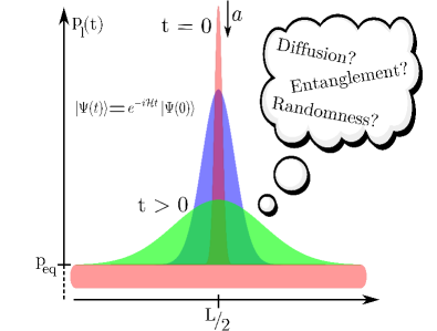
In this paper, we study these questions and focus, as a first step, on a nonintegrable version of the spin-$1/2$ Heisenberg model in one dimension. While integrability can be certainly broken in many different ways, we do so by taking into account an additional interaction between next-nearest neighbors. For this model, we analyze the real-time and real-space dynamics of magnetization as resulting for a convenient class of nonequilibrium initial states. These states have been introduced in steinigeweg2017_1 , are pure, and realize a sharp density peak on top of homogeneous many-particle background at any temperature, as illustrated in Fig. 1. Since this class of initial states allows for changing internal degrees of freedom without modifying the initial density profile, we are able to investigate whether and in how far such internal details influence the real-time broadening. Here, an useful concept is typicality of pure states. It implies in the case of internal randomness a dynamical behavior in agreement with the equilibrium correlation function and allows us to perform large-scale numerical simulations in the framework of linear response.

Summarizing our main results in a nutshell, we show that signatures of diffusion are equally pronounced for the integrable and nonintegrable case. We further find in both cases a strong difference between the dynamics of typical states (with internal randomness) and untypical states (without any randomness). We further provide an explanation of this difference by a detailed analysis of entanglement and local density of states.

The rest of this paper is structured as follows. First, we introduce in Sec. II the Heisenberg spin-1/2 chain with an integrability-breaking interaction between neighbors at next-nearest sites. Then, we discuss the framework in Sec. III and give an overview over our observables and initial states, linear response, and diffusion. Afterward, we discuss in Sec. IV the concept of typicality and our numerical approach. Eventually, we present our results in Secs. V and VI and particularly analyze integrability vs. nonintegrability, typical vs. untypical states, as well as entanglement and local density of states. We finally close with a summary and conclusions in Sec. VII and provide additional information in the appendix.

II Model

The present paper studies the one-dimensional spin-$1/2$ XXZ chain, where the standard model is extended to incorporate also interactions between next-nearest neighbors. The Hamiltonian $\mathcal{H}=\mathcal{H}_{\text{XXZ}}+\mathcal{H}^{\prime}$ with periodic boundary conditions reads

$$\mathcal{H}_{\text{XXZ}}=J\sum_{l=1}^{L}\left(S_{l}^{x}S_{l+1}^{x}+S_{l}^{y}S_{l+1}^{y}+\Delta S_{l}^{z}S_{l+1}^{z}\right)\ ,$$ (1)

$$\mathcal{H}^{\prime}=J\sum_{l=1}^{L}\Delta^{\prime}S_{l}^{z}S_{l+2}^{z}\ ,$$ (2)

where $S_{l}^{i}$, $i\in\{x,y,z\}$ are spin-$1/2$ operators at site $l$, $L$ is the total number of sites, and $J>0$ is the antiferromagnetic exchange constant. Using the Jordan-Wigner transformation, $\mathcal{H}$ can be mapped to an one-dimensional model of spinless fermions with nearest and next-nearest neighbor interactions, where the strength of the interactions is set by $\Delta$ and $\Delta^{\prime}$, respectively. In the case $\Delta^{\prime}=0$, the model is integrable in terms of the Bethe Ansatz, with the energy current being exactly conserved zotos1997 ; kluemper2002 , whereas integrability is broken for any $\Delta^{\prime}\neq 0$.

The difference between the integrable and the non-integrable model is also reflected in the level-spacing distribution $P(s)$, see Fig. 2.

Figure 2: (Color online) Level-spacing distribution $P(s)$ of the spin-$1/2$ XXZ chain with $L=20$, for a single symmetry subsector labeled by the quantum numbers $S^{z}=1$ and $k=1$. In the integrable case $\Delta^{\prime}=0$, the distribution is well described by a Poissonian, whereas for the non-integrable case $\Delta=\Delta^{\prime}=1.5$, one observes Wigner statistics.

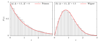
For $\Delta^{\prime}=0$ [Fig. 2 (a)], $P(s)$ exhibits Poissonian behavior, in contrast to the non-integrable case $\Delta=\Delta^{\prime}\neq 0$ [Fig. 2 (b)], where $P(s)$ obeys the quantum chaotic Wigner distribution. Note that a proper analysis of $P(s)$ requires an unfolding of the spectrum santos2004 ; santos2010 . Moreover, here we restrict ourselves to a single subsector of $\mathcal{H}$ with magnetization $S^{z}=1$ and momentum $k=1$, in order to eliminate all trivial symmetries. Note, however, that for the rest of this paper we always consider the full Hilbert space without any restriction.

III Framework

III.1 Observables and initial states

In this paper, the real-time dynamics of local occupation numbers

$$n_{l}=S_{l}^{z}+\frac{1}{2}$$ (3)

is studied. To this end, expectation values of the form

$$p_{l}(t)=\text{Tr}[\rho(t)\ n_{l}]$$ (4)

are evaluated, where $\rho(t)$ is the density matrix at time $t$,

$$\rho(t)=e^{-i\mathcal{H}t}\ket{\psi(0)}\bra{\psi(0)}e^{i\mathcal{H}t}\ ,$$ (5)

and $\ket{\psi(0)}$ is a pure state. The special class of (normalized) non-equilibrium initial states $\ket{\psi(0)}$ considered in this paper are constructed as

$$\ket{\psi(0)}\propto(n_{L/2}-a)\ket{\Phi}\ ,\quad\ket{\Phi}=\sum_{k=1}^{2^{L}}c_{k}\ket{\varphi_{k}}\ ,$$ (6)

where $c_{k}$ are complex coefficients and $a\geq 0$ is a real number. The states $\ket{\varphi_{k}}$ denote the common eigenbasis of all $n_{l}$, i.e. the Ising basis. The operator $n_{L/2}$ acts as a projection onto all states with a spin-up in the middle of the chain. In the case $a=0$, we consequently have $p_{L/2}(0)=1$ by construction. By choosing $a>0$, it is however straightforward to adjust this initial amplitude. (For more details, see the appendix). For the particular choice of all coefficients $c_{k}$ being the same in Eq. (6), we moreover find $p_{l\neq L/2}=p_{\text{eq}}=1/2$. Thus, one ends up with an initial density profile which has a central peak in the middle of the chain, on top of a homogeneous many-particle background, see Fig. 1. However, exactly the same density profile arises if real and imaginary part of the $c_{k}$ are randomly drawn from a Gaussian distribution with zero mean (according to the unitary invariant Haar measure bartsch2009 ; bartsch2011 ).

Although not distinguishable at $t=0$, it has been demonstrated steinigeweg2017_1 that the dynamics for times $t>0$ can depend strongly on whether $\ket{\psi(0)}$ is a “typical” state with random $c_{k}$ or an “untypical” state where all $c_{k}$ are the same. A central aim of the present paper is to understand the crucial differences between these two choices of initial states. To this end, the states are analyzed in terms of their local density of states, their internal randomness, as well as their entanglement. In this respect, it is important to note that, for all $c_{k}$ being the same, it is possible to write $\ket{\psi(0)}$ as a product state with a spin-up state $\ket{\uparrow}$ in the middle of the chain and a spin-up/spin-down superposition at all other sites,

$$\ket{\psi(0)}\propto\dots(\ket{\uparrow}+\ket{\downarrow})\otimes\ket{\uparrow}\otimes(\ket{\uparrow}+\ket{\downarrow})\dots\ .$$ (7)

On the other hand, for completely or at least partially random coefficients $c_{k}$, such a full product structure is absent.

III.2 Kubo Formula

Within the framework of linear response theory (LRT), transport coefficients can be computed from current-current correlation functions

$$\langle j(t)j\rangle=\text{Tr}[j(t)j\rho_{\text{eq}}]\ ,$$ (8)

which are evaluated within the canonical equilibrium ensemble $\rho_{\text{eq}}=e^{-\beta H}/{\cal Z}$ at inverse temperature $\beta=1/T$ kubo1957 ; luttinger1964 ; mahan1990 , where $\mathcal{Z}=\text{Tr}[e^{-\beta{\cal H}}]$ is the partition function. The time argument has to be understood with respect to the Heisenberg picture.

In the present paper, our focus is on the transport of magnetization and the operator $j$ therefore denotes the spin current. Since total magnetization $S^{z}=\sum_{l}S_{l}^{z}$ is conserved, $[\mathcal{H},S^{z}]=0$, the spin current $j$ is well-defined and follows from the lattice continuity equation

$$\frac{\text{d}}{\text{d}t}S_{l}^{z}=i[\mathcal{H},S_{l}^{z}]=j_{l-1}-j_{l}\ .$$ (9)

Thus, for the Hamiltonian $\mathcal{H}$, as defined in Eqs. (1) and (2), $j$ takes on the well-known form

$$j=\sum_{l=1}^{L}j_{l}=J\sum_{l=1}^{L}(S_{l}^{x}S_{l+1}^{y}-S_{l}^{y}S_{l+1}^{x})\ ,$$ (10)

which is exactly conserved only in the case $\Delta=\Delta^{\prime}=0$. In LRT, the connection between transport properties and current autocorrelations is given by the Kubo formula which, in case of the spin current, can be written as

$$\sigma(\omega)=\frac{1-e^{-\beta\omega}}{\omega L}\int\limits_{0}^{\infty}e^{i\omega t}\ \langle j(t)j\rangle\ \text{d}t\ ,$$ (11)

where $\sigma(\omega)$ is the conductivity at the inverse temperature $\beta$. Often, $\text{Re}\,\sigma(\omega)$ is decomposed into a $\delta$ function at $\omega=0$ and a part for frequencies $\omega\neq 0$,

$$\text{Re}\ \sigma(\omega)=\bar{C}\delta(\omega)+\sigma_{\text{reg}}(\omega)\ ,$$ (12)

where $\bar{C}$ is the so-called Drude weight zotos2004 ; heidrichmeisner2003 ; heidrichmeisner2007 . In fact, $\bar{C}$ can be directly related to the long-time limit of the current autocorrelation function $C(t)$ steinigeweg2009_1 ; karrasch2012 ; karrasch2013 ; steinigeweg2014 ; steinigeweg2015 ; karrasch2014_1 ,

$$\bar{C}=\int_{t_{1}}^{t_{2}}\text{d}t\ \frac{C(t)}{t_{2}-t_{1}}\ ,$$ (13)

with $C(t)=\text{Re}\langle j(t)j\rangle/L$. Here, $t_{1}$ and $t_{2}$ are selected from a region where $C(t)$ has decayed to its long-time value $C(t\rightarrow\infty)\geq 0$. Thus, a nonzero Drude weight exists whenever the current is at least partially conserved and indicates ballistic transport zotos2004 ; heidrichmeisner2003 ; heidrichmeisner2007 . In cases where the Drude weight vanishes and transport is not ballistic in the thermodynamic limit, the dc conductivity $\sigma_{\text{dc}}=\sigma_{\text{reg}}(\omega\rightarrow 0)$ is of interest and follows from a zero-frequency Fourier transform of $C(t)$ prelovsek2004 ; steinigeweg2009_1 ; steinigeweg2015 ; karrasch2014_1 ; karrasch2014_2 ,

$$\sigma_{\text{dc}}=\beta\int_{0}^{t_{\text{max}}}\text{d}t\ C(t)\ .$$ (14)

Since the Drude weight $\bar{C}$ will always be nonzero for a finite system, the integral in Eq. (14) diverges in the limit $t_{\text{max}}\rightarrow\infty$ steinigeweg2009_1 . Therefore the cutoff time $t_{\text{max}}<\infty$ is chosen to be finite, but long enough to ensure that $\sigma_{\text{dc}}$ is effectively independent of the particular choice of $t_{\text{max}}$. Note that there exist different definitions for $\bar{C}$ and $\sigma_{\text{dc}}$ in the literature, with additional prefactors $\pi$, $2\pi$ and $\beta$.

III.3 Diffusion

As discussed in Sec. III.2, a finite Drude weight immediately implies ballistic transport. However, a vanishing Drude weight not necessarily leads to diffusive behavior. In this subsection, we therefore summarize the conditions for diffusion.

Defined on a discrete lattice, the dynamics of some density (here magnetization density) $p_{l}$ is said to be diffusive if it fulfills a diffusion equation of the form michel2005 ; steinigeweg2007

$$\frac{\text{d}}{\text{d}t}\ p_{l}(t)=D\left[p_{l-1}(t)-2p_{l}(t)+p_{l+1}(t)\right]\ ,$$ (15)

where $D$ is the time-independent diffusion constant. For this equation, one finds a specific solution for the time and site dependence of $p_{l}(t)$,

$$p_{l}(t)-p_{\text{eq}}=\frac{1}{2}\exp(-2Dt)\,{\cal B}_{l-L/2}(2Dt)\ ,$$ (16)

with ${\cal B}_{l}(t)$ being the modified Bessel function of the first kind. This lattice solution can be well approximated by the corresponding continuum solution

$$p_{l}(t)-p_{\text{eq}}=\frac{1}{2}\frac{1}{\sqrt{2\pi}\Sigma(t)}\exp\left[-\frac{(l-L/2)^{2}}{2\Sigma^{2}(t)}\right]\ ,$$ (17)

where the spatial variance is given by

$$\Sigma^{2}(t)=2Dt\ .$$ (18)

Note that, in the limit $\Sigma(t\rightarrow 0)$, Eq. (17) becomes a $\delta$ function located at lattice site $l=L/2$, which coincides with our initial density profile.

Generally, the spatial variance $\Sigma^{2}(t)$ of an arbitrary distribution is given by

$$\Sigma^{2}(t)=\sum_{l=1}^{L}l^{2}\ \delta p_{l}(t)-\left[\sum_{l=1}^{L}l\ \delta p_{l}(t)\right]^{2}\ ,$$ (19)

where $\delta p_{l}(t)\propto[p_{l}(t)-p_{\text{eq}}]$ and $\sum_{l=1}^{L}\delta p_{l}(t)=1$. Thus, in the case of diffusive transport, the variances from Eqs. (18) and (19) exactly coincide with each other, and our non-equilibrium dynamics should be described by Gaussians as given in Eq. (17).

However, a time-independent diffusion constant, and the existence of diffusion as such, is questionable in view of unitary Schrödinger dynamics michel2005 . Moreover, as we will also see during the discussion of our results, it might not always be appropriate to draw conclusions only on the basis of the real-space data. Therefore, we here introduce an useful scheme: A Fourier transform of the diffusion equation in Eq. (15) yields

$$\frac{\text{d}}{\text{d}t}\ p_{q}(t)=-2(1-\cos q)D_{q}(t)p_{q}(t)\ ,$$ (20)

where we additionally allow for a time- and momentum-dependent $D_{q}(t)$, and momentum $q$ takes on the values $q=2\pi k/L$ with $k=0,1,\ldots,L-1$. Rearranging Eq. (20) and using the abbreviation $\tilde{q}^{2}=2(1-\cos q)$ then gives the generalized diffusion coefficient steinigeweg2011_1

$$D_{q}(t)=\frac{\text{d}/\text{d}t\ p_{q}(t)}{-\tilde{q}^{2}\ p_{q}(t)}\ .$$ (21)

In the case of diffusive transport, the behavior of $D_{q}(t)$ can be qualitatively understood as follows. On the one hand, $D_{q}(t)\propto t$ always increases linearly for sufficiently short times steinigeweg2011_1 . On the other hand, above the mean free time $\tau$ and above the mean free path $\lambda$, i.e., $t>\tau$ and $\pi/q>\lambda$, $D_{q}(t)$ eventually turns into a plateau with $D_{q}(t)\approx\text{const}$, which marks the hydrodynamic regime.

Eventually, it is also instructive to connect $D_{q}(t)$ to linear response theory. Assuming $p_{q}(t)\propto\text{Re}\,\langle S_{q}^{z}(t)S_{-q}^{z}\rangle$, where $S_{q}^{z}=\sum_{l}e^{iql}S_{l}^{z}/\sqrt{L}$, it follows in the limit $q\rightarrow 0$ that steinigeweg2011_1

$$D(t)=\frac{1}{\chi}\int_{0}^{t}\text{d}t^{\prime}\ C(t^{\prime})\ ,$$ (22)

where the static susceptibility is $\chi=1/4$ in the limit $\beta\rightarrow 0$. Under the above assumption, $D(t)$ is also related to the time derivative of the spatial variance steinigeweg2009_2 ; yan2015 ; luitz2017 ; karrasch2017 ,

$$\frac{\text{d}}{\text{d}t}\Sigma^{2}(t)=2D(t)\ .$$ (23)

The time dependence of $D(t)$ can be summarized as follows. For the non-interacting case $\Delta=\Delta^{\prime}=0$, we have $[\mathcal{H},j]=0$, leading to $D(t)\propto t$ such that $\Sigma^{2}(t)\propto t^{2}$ scales ballistically for all t. Such ballistic behavior is also known to occur for partial current conservation at $\Delta<1$ and $\Delta^{\prime}=0$ shastry1990 ; castella1995 ; narozhny1998 ; zotos1999 ; heidrichmeisner2003 ; fujimoto2003 ; benz2005 ; prosen2011 ; prosen2013 ; herbrych2011 ; karrasch2012 ; karrasch2013 ; steinigeweg2014 ; steinigeweg2015 ; ilievski2017 . In the case of diffusive transport, $D(t)=\text{const}$ and $\Sigma(t)\propto t$. Moreover, a process is called superdiffusive if $\Sigma(t)\propto t^{\alpha}$ with $\alpha\in]1,2[$ and subdiffusive for $\alpha\in]0,1[$. However, it is important to note that $D(t)$ yields no information beyond the mere width of density profiles.

IV Dynamical Quantum Typicality

IV.1 Current-current correlations

The concept of typicality gemmer2003 ; goldstein2006 ; popescu2006 ; reimann2007 ; sugiura2012 ; sugiura2013 ; elsayed2013 ; iitaka2003 ; iitaka2004 ; white2009 ; monnai2014 ; reimann2016 states that a single pure state can have the same “properties” as the full statistical ensemble. Remarkably, this concept does not require eigenstate thermalization deutsch1991 ; srednicki1994 ; rigol2008 and also applies to the dynamics of expectation values. In particular, dynamical quantum typicality (DQT) has turned out to be a powerful method for the accurate calculation of real-time current correlation functions in huge Hilbert spaces elsayed2013 ; steinigeweg2014 ; steinigeweg2015 ; steinigeweg2016 .

The main idea is to replace the trace $\text{Tr}[\bullet]$ in Eq. (8) by a single scalar product $\bra{\Phi}\bullet\ket{\Phi}$, where $\ket{\Phi}$ is a pure state, randomly drawn from the full Hilbert space according to the unitary invariant Haar measure bartsch2009 ; bartsch2011 . The current autocorrelation function can then be written as elsayed2013 ; steinigeweg2014 ; steinigeweg2015 ; steinigeweg2016

$$C(t)=\frac{\text{Re}\bra{\Phi}j(t)\ j\ e^{-\beta\mathcal{H}}\ket{\Phi}}{L\bra{\Phi}e^{-\beta\mathcal{H}}\ket{\Phi}}+\epsilon(\ket{\Phi})\$$ (24)

or, equivalently, as

$$C(t)=\frac{\text{Re}\bra{\phi(t)}j\ket{\varphi(t)}}{L\braket{\phi(0)}{\phi(0)}}+\epsilon(\ket{\Phi})\ ,$$ (25)

where we have introduced the two auxiliary pure states

$$\ket{\phi(t)}=e^{-i\mathcal{H}t}e^{-\beta{\cal H}/2}\ket{\Phi}\ ,$$ (26)

$$\ket{\varphi(t)}=e^{-i\mathcal{H}t}j\ e^{-\beta{\cal H}/2}\ket{\Phi}\ ,$$ (27)

which only differ by the additional current operator in Eq. (27). It is important to note that the error in Eq. (24) scales as $\epsilon\propto 1/\sqrt{d}$ for $\beta\rightarrow 0$, with $d=2^{L}$ being the dimension of the Hilbert space. Thus, for the large system sizes we are interested in, this error is negligibly small and the typicality approximation can be regarded as practically exact. Furthermore, the time dependence, e.g. of $\ket{\phi(t)}$, can be conveniently evaluated by iteratively solving the real-time Schrödinger equation (see Sec. IV.3).

IV.2 Density-density correlations

Concerning the dynamics of local occupation numbers, we can perform the following calculation steinigeweg2017_1 ; steinigeweg2017_2 . We start from an equilibrium correlation function in the limit $\beta\to 0$,

$$\mathcal{C}_{l}(t)=2\langle n_{L/2}\ n_{l}(t)\rangle =2\frac{\text{Tr}[n_{L/2}\ n_{l}(t)]}{2^{L}}$$ (28)

$$=2\frac{\text{Tr}[n_{L/2}\ n_{l}(t)\ n_{L/2}]}{2^{L}}\ ,$$ (29)

where the cyclic invariance of the trace and the projection property $n_{L/2}^{2}=n_{L/2}$ has been exploited. According to typicality, also this expression can be rewritten using a randomly drawn pure state $\ket{\Phi}$,

$$\mathcal{C}_{l}(t) =2\frac{\bra{\Phi}n_{L/2}\ n_{l}(t)\ n_{L/2}\ket{\Phi}}{\braket{\Phi}{\Phi}}+\epsilon(\ket{\Phi})$$ (30)

$$=\frac{\bra{\psi}e^{i\mathcal{H}t}\ n_{l}\ e^{-i\mathcal{H}t}\ket{\psi}}{\braket{\psi}{\psi}}\ ,$$ (31)

where we have used the definition of our initial state in Eq. (6) and $\braket{\psi}{\psi}=\braket{\Phi}{\Phi}/2$. Moreover, we have dropped the error $\epsilon$ for clarity. Since $\ket{\psi(t)}=e^{-i\mathcal{H}t}\ket{\psi}$, we finally find

$$\mathcal{C}_{l}(t)=\frac{\bra{\psi(t)}n_{l}\ket{\psi(t)}}{\braket{\psi(0)}{\psi(0)}}=p_{l}(t)\ .$$ (32)

Thus, it follows that, although the initial states in Eq. (6), have to be considered as far from equilibrium, the resulting non-equilibrium dynamics is directly related to an equilibrium correlation function.

IV.3 Forward propagation of pure states

Using exact diagonalization (ED), it is possible to compute the time evolution of a pure state via

$$\ket{\psi(t)}=\sum_{n}e^{iE_{n}t}c_{n}\ket{n}\ ,$$ (33)

where $\ket{n}$ are eigenvectors of the Hamiltonian with corresponding eigenvalues $E_{n}$, and $c_{n}=\braket{n}{\psi(0)}$ denotes the overlap of $\ket{n}$ and $\ket{\psi(0)}$. However, the exponential growth of the Hilbert space represents a natural limitation of ED. Usually, this growth is at least partially compensated by exploiting the symmetries of the Hamiltonian. To repeat, the Hamiltonian $\mathcal{H}$ in Eqs. (1) and (2) conserves total magnetization $S^{z}=\sum_{l}S_{l}^{z}$. Moreover, it is invariant under translation by one lattice site and crystal momentum $k$ becomes a good quantum number. Thus, it is in principle possible to divide the Hilbert space into subspaces, classified by $S^{z}$ and $k$. However, since the operator $n_{L/2}$ in the definition (6) of the initial states does not respect translational invariance, it becomes less profitable to use this symmetry for our calculations. In any case, ED is limited to systems with a maximum of $L\sim 20$ sites.

Therefore, we proceed differently in the present paper and rely on a forward propagation of $\ket{\psi(t)}$ in real time. Such a propagation can be done by means of a fourth-order Runge-Kutta (RK4) scheme elsayed2013 ; steinigeweg2014 ; steinigeweg2015 ; steinigeweg2016 or by more sophisticated methods such as Chebyshev polynomials weisse2006 ; dobrovitski2003 or Trotter decompositions steinigeweg2017_1 ; steinigeweg2017_2 ; deReadt2006 . Using these methods, no diagonalization of $\mathcal{H}$ is needed and, since $\mathcal{H}$ is usually relatively sparse, the matrix-vector multiplications can be implemented very memory-efficient. In this paper, we use a RK4 method for chains up to $L\leq 26$ sites. For longer chains, we employ a Trotter product formula which allows us to treat systems with as many as $L=36$ spins. For this $L$, the largest subsector with $S^{z}=0$ has dimension $d\approx 10^{10}$ and is several orders of magnitude larger than the matrices treatable by state-of-the-art ED.

V Dynamics of Typical and Untypical States

We now present our numerical results. As a first step in Sec. V.1, we study current autocorrelations and Drude weights, i.e. results obtained within the framework of LRT. These results will be useful in the discussion of the non-equilibrium dynamics in the subsequent Sec. V.2.

V.1 Current autocorrelations and Drude weights

Figure 3: (Color online) (a) Current autocorrelation function $C(t)$ up to times $tJ=100$ and for systems with $L=26$ and $33$ sites (arrows). Data is shown for the integrable case $\Delta^{\prime}=0$ with $\Delta=0.5$ and $\Delta=1$ as well as for the non-integrable case $\Delta=\Delta^{\prime}=0.5$. (b) Finite-size scaling of the Drude weight $\bar{C}$ for selected values of $\Delta$ and $\Delta^{\prime}$. For the integrable cases $\Delta^{\prime}=0$, the data is obtained according to Eq. (13) and from the finite time interval $[t_{1}J,t_{2}J]=[70,100]$, cf. Fig. 3 (a), whereas for $\Delta=\Delta^{\prime}=0.5$, the interval $[t_{1}J,t_{2}J]=[250,300]$ is chosen. The dashed lines are linear fits to the data. In the case $\Delta=0.5$, $\Delta=0$ we additionally show an analytic bound for $\bar{C}$ prosen2011 ; prosen2013 . Note that $L=33$ data for the integrable cases have been taken from Ref. steinigeweg2014 .

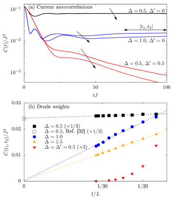
According to Eq. (13), the Drude weight $\bar{C}$ is related to the long-time limit of the current-current correlation function $C(t)$. Since $\bar{C}>0$ for finite systems, a careful finite-size scaling needs to be performed, in order to draw reliable conclusions on $\bar{C}$ in the thermodynamic limit. Therefore, in Fig. 3 (a), $C(t)$ is shown for different choices of $\Delta$ and $\Delta^{\prime}$ and for various chain lengths $L$.

While it is certainly convenient to start our discussion with the integrable model, i.e. $\Delta^{\prime}=0$, we should stress that corresponding results and a detailed discussion can be found already in Ref. steinigeweg2014 . For $\Delta^{\prime}=0$ and at the isotropic point $\Delta=1$, one observes that, after an initial decay, $C(t)$ reaches an approximately constant long-time value for times $tJ\gtrsim 50$. Moreover, this long-time value decreases for increasing system size. On the contrary, for $\Delta^{\prime}=0$ and $\Delta=0.5$, a significant dependence of $C(t)$ and its long-time value on $L$ is not visible. Most important, however, in the case of a non-zero next-nearest neighbor interaction $\Delta^{\prime}=0.5$, $C(t)$ decays to substantially smaller values. In fact, even at times $tJ=300$ (not shown), $C(t)$ has not yet reached its stationary value.

In Fig. 3 (b), we show a finite-size scaling of the Drude weight $\bar{C}$. For the integrable model, the data is obtained according to Eq. (13) and from the finite time interval $[t_{1}J,t_{2}J]=[70,100]$, as indicated in Fig. 3 (a). Linear extrapolations of the data towards the thermodynamic limit are also depicted. In the case $\Delta=0.5$, one observes that the Drude weight converges towards a finite value $\bar{C}>0$, in quantitative agreement with analytical results prosen2011 ; prosen2013 . For the case $\Delta\geq 1$, the linear fit clearly suggest a vanishing Drude weight $\bar{C}=0$ for $L\rightarrow\infty$. For the non-integrable model $\Delta=\Delta^{\prime}=0.5$, $\bar{C}$ is extracted from the interval $[t_{1}J,t_{2}J]=[250,300]$. As mentioned, $C(t)$ has not completely decayed even at these long times such that the data has to be understood as an upper bound for $\bar{C}$. Apparently, this upper bound decreases faster than a power law with increasing $L$ and is most likely expected to vanish for $L\rightarrow\infty$, as expected for non-integrable systems heidrichmeisner2003 ; heidrichmeisner2007 .

V.2 Real-space dynamics of typical states

Figure 4: (Color online) Time-space density plot of occupation numbers $p_{l}(t)$ for a typical initial state $\ket{\psi(0)}$ in the XXZ spin-$1/2$ chain with $L=36$ sites and different anisotropies $\Delta=\Delta^{\prime}=1.5$, $1$, and $0.5$ [(a) - (c)].

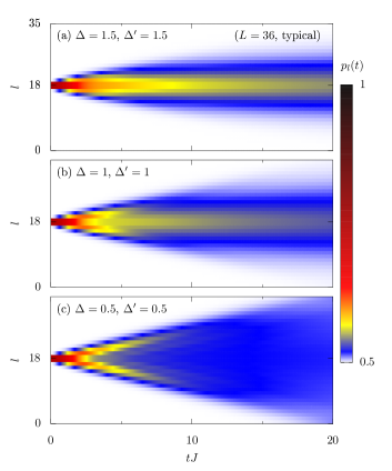
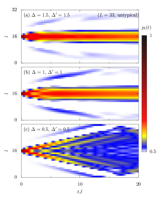
To start the discussion of non-equilibrium dynamics in real space and time, we first consider typical initial states. In Fig. 4, a time-space density plot of occupation numbers $p_{l}(t)$ is shown for a chain with $L=36$ sites and different anisotropies $\Delta=\Delta^{\prime}=1.5$, $1$, $0.5$, up to times $tJ=20$. For all parameters shown, one observes that the sharp initial peak broadens monotonically with time. In the case of weak interactions [Fig. 4 (c)], this broadening is still linear due to a long mean free time $\tau=\mathcal{O}(10)$. This can be also understood with respect to the current autocorrelation [see Fig. 3 (a)], which is not fully decayed at this time scale. On the other hand, for larger anisotropies, the broadening of the density profiles is non-linear and significantly slower, which can be explained by the increased scattering of particles.

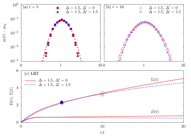
For a more detailed analysis, Fig. 5 (a) shows the density profile $p_{l}(t)$ for fixed times $tJ=5$ and $10$ in a semi-log plot, both for the integrable case with $\Delta=1.5$, $\Delta^{\prime}=0$ and the non-integrable case with $\Delta=\Delta^{\prime}=1.5$. One observes that the data is remarkably well described by Gaussians over several orders of magnitude. Moreover, there are no significant differences between the integrable and the non-integrable model visible. Thus, we conclude that, for a large anisotropy $\Delta=1.5$, the dynamics of our typical initial state is basically unaffected by the strong additional next-nearest neighbor interaction, which can be also explained analytically on the basis of projection operator techniques steinigeweg2011_2 .

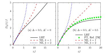
In Fig. 5 (b), we additionally compare the non-equilibrium dynamics to results from LRT. To this end, the time-dependent diffusion coefficient $D(t)$ and the corresponding width $\Sigma(t)$ [see Eqs. (22) and (23)] are shown for $L=36$ sites. These LRT results are compared to the values of $\Sigma(t)$ according to Eq. (19), i.e., as directly extracted from the density profiles in Fig. 5 (a). Overall, we find a convincing agreement between the non-equilibrium dynamics and LRT. Most importantly, however, one observes $D(t)\approx\text{const}$ at the time scales depicted steinigeweg2009_1 ; karrasch2014_2 . Thus, $\Sigma(t)\propto\sqrt{t}$, both for $\Delta^{\prime}=0$ and $\Delta^{\prime}\neq 0$. This scaling as well as the Gaussian form of the density profiles clearly indicate diffusive transport in this parameter regime, irrespective of the model being integrable or non-integrable. This is a central result of our paper.

Figure 5: (Color online) (a) and (b) Density profile $p_{l}(t)$ with respect to site $l$ at fixed times $tJ=5$ and $10$ for $\Delta=1.5$, $\Delta^{\prime}=0$ as well as $\Delta=\Delta^{\prime}=1.5$ shown in a semi-log plot. The difference between the integrable and non-integrable model are remarkably small and the data is well described by Gaussian fits over several orders of magnitude. (c) Time-dependent diffusion coefficient $D(t)$ and profile width $\Sigma(t)$ according to LRT for $L=34$ ($\Delta^{\prime}=0$) steinigeweg2015 and $L=36$ ($\Delta^{\prime}=1.5$). For comparison, the symbols represent the width $\Sigma(t)$ of the non-equilibrium data in (a) and (b) and are in convincing agreement with LRT.

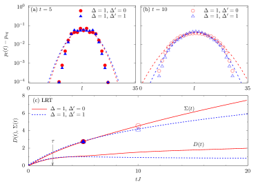
Next, let us discuss the case of smaller $\Delta$ and $\Delta^{\prime}$ in more detail. Completely analogous to Fig. 5, the density profiles $p_{l}(t)$ for $\Delta=1$, $\Delta^{\prime}=0$ and $\Delta=\Delta^{\prime}=1$ are shown in Fig. 6 (a) for fixed times $tJ=5$ and $10$. Compared to the previous case of larger anisotropies, we observe that it is not possible anymore to describe the density profiles by Gaussian fits, both for the integrable and the non-integrable model. Furthermore, in contrast to the case of larger anisotropies, the time dependence of $D(t)$ and $\Sigma(t)$ exhibits significant differences between $\Delta^{\prime}=0$ and $\Delta^{\prime}\neq 0$. On the one hand, the nonconstant $D(t)$ in the integrable case is clearly inconsistent with diffusion but rather suggests superdiffusive behavior znidaric2011 ; steinigeweg2012 ; ljubotina2017 , see also khait2016 . In contrast, at low temperatures, signatures of diffusive behavior have been reported sirker2009 ; sirker2011 ; grossjohann2010 . On the other hand, for $\Delta^{\prime}\neq 0$, one observes $D(t)\approx\text{const}$ as well as $\Sigma(t)\propto\sqrt{t}$. However, due to the non-Gaussian density profiles in Fig. 6 (a), one might argue that the possibility of diffusion is still ruled out. It should be noted, however, that for times below the mean free time $\tau J\approx 2$ one finds $D(t)\propto t$ [see Fig. 6 (b)] and only for times $t>\tau$ the diffusion coefficient $D(t)$ turns into a constant plateau. Thus, at short times, the sharp initial density profile broadens ballistically. Consequently, even if there exists diffusive behavior at longer time scales, one generally cannot expect clean Gaussian profiles but rather a superposition of such Gaussians.

Figure 6: (Color online) (a) Density profile $p_{l}(t)$ with respect to site $l$ at fixed times $tJ=5$, $10$ for $\Delta=1$, $\Delta^{\prime}=0$ and $\Delta=\Delta^{\prime}=1$, shown in a semi-log plot. (b) Time-dependent diffusion coefficient $D(t)$ and profile width $\Sigma(t)$ according to LRT for $L=34$ ($\Delta^{\prime}=0$) steinigeweg2014 and $L=36$ ($\Delta^{\prime}=1$). The symbols represent the width $\Sigma(t)$ of the non-equilibrium data in (a). $\tau$ approximately marks the mean free time.

V.3 Momentum-space dynamics of typical states

Due to the above reasoning, it is sometimes not sufficient to draw conclusions on diffusive or non-diffusive behavior only on the basis of the real-space data, with single-site resolution below the mean free path. Consequently, we proceed also in a different way and analyze the generalized diffusion coefficient $D_{q}(t)$, as introduced in Eq. (21).

In Figs. 7 (a) and (b), the generalized diffusion coefficient $D_{q}(t)$ is shown for large anisotropies $\Delta=1.5$, $\Delta^{\prime}=0$ and $\Delta=\Delta^{\prime}=1.5$. Non-equilibrium results at momentum $q/(2\pi/L)=1$ and $2$ are compared to LRT for $q=0$, up to times $tJ=15$. Overall, the integrable model in Fig. 7 (a) and the non-integrable model in Fig. 7 (b) behave very similarly. In both cases, one observes that at least the first three momenta feature a plateau with $D_{q}(t)\approx\text{const}$, which is a clear signature of diffusion and confirms our earlier conclusion. Note that the slight increase of $D_{q}(t)$ in Fig. 7 (a) is not necessarily a finite-size effect karrasch2014_2 ; steinigeweg2015 .

Figure 7: (Color online) Generalized diffusion coefficient $D_{q}(t)$, obtained from the non-equilibrium density profiles according to Eq. (21) for momenta $q/(2\pi/L)=k$ and $L=36$. As a comparison, $D_{q=0}(t)$ according to LRT is shown, for $L=34$ ($\Delta^{\prime}=0$) steinigeweg2015 and $L=36$ ($\Delta^{\prime}\neq 0$). Other parameters: (a) $\Delta=1.5$, $\Delta^{\prime}=0$; (b) $\Delta=\Delta^{\prime}=1.5$; (c) $\Delta=1$, $\Delta^{\prime}=0$; (d) $\Delta=1$, $\Delta^{\prime}=1$.

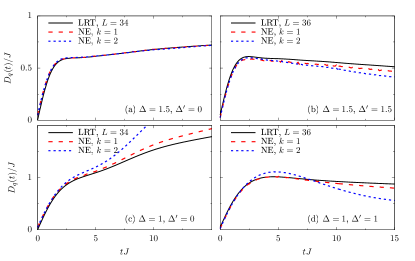
Now, we come back to the case of smaller anisotropies. In Fig. 7 (c), $D_{q}(t)$ is depicted for the integrable case $\Delta=1$, $\Delta^{\prime}=0$, while Fig. 7 (d) shows the non-integrable case $\Delta=\Delta^{\prime}=1$. For $\Delta^{\prime}=0$, one clearly observes that the diffusion coefficient increases with time for all $q\geq 0$. Moreover, even for the smallest nonzero momentum $q/(2\pi/L)=1$, we see deviations between $q\neq 0$ and $q=0$. For $\Delta^{\prime}\neq 0$, $D_{q}(t)$ behaves significantly different. For $q=0$, we have $D_{q}(t)\approx\text{const}$, which is accurately reproduced at least for $q/(2\pi/L)=1$. For larger wave vectors, however, we are unable to find a plateau with constant $D_{q}(t)$. Thus, compared to the case of larger anisotropies [Figs. 7 (a) and (b)], the hydrodynamic regime is shifted to smaller momenta if $\Delta$, $\Delta^{\prime}$ is decreased.

Based on the data in Fig. 7, we conclude that the real-time dynamics of typical states in the XXZ chain shows diffusive behavior, not only for large anisotropies $\Delta=1.5$ but also for smaller $\Delta=1$, if integrability is broken due to an additional next-nearest neighbor interaction $\Delta^{\prime}>0$. This is another main result of the present paper. Note that a similar result is likely to appear for even smaller anisotropies, e.g., $\Delta=\Delta^{\prime}=0.5$. However, due to a large mean free path, we are not able to draw reliable conclusions in this parameter regime. More details on this issue are given in the appendix.

V.4 Real-space dynamics of untypical states

Now, we turn to our study of untypical initial states, where the coefficients $c_{k}$ in Eq. (6) are all chosen to be equal. Figure 8 shows a time-space density plot of occupation numbers $p_{l}(t)$ for a chain with $L=33$ sites. Completely analogous to Fig. 4, panels (a) - (c) show results for $\Delta=\Delta^{\prime}=1.5$, $1$, and $0.5$. First of all, one observes that the time dependence of the density profiles strongly differs from the case of typical initial states. On the one hand, for large interactions $\Delta$ [see Fig. 8 (a)], the broadening is basically frozen and the density profile is very narrow even at times $tJ=20$, similar to gobert2005 . On the other hand, for small interactions $\Delta$ [see Fig. 8 (c)], one observes pronounced jets which propagate freely until they eventually hit the boundary at times $tJ\sim 20$. Such a behavior of untypical states has been already found for the integrable model $\Delta^{\prime}=0$ steinigeweg2017_1 . Our present results clearly show that this behavior is stable against perturbations $\Delta^{\prime}\neq 0$.

Figure 8: (Color online) Time-space density plot of occupation numbers $p_{l}(t)$for an untypical initial state $\ket{\psi(0)}$ in the XXZ spin-$1/2$ chain with $L=33$ sites and different anisotropies $\Delta=\Delta^{\prime}=1.5$, $1$, and $0.5$ [(a) - (c)].

VI Properties of Typical and Untypical States

In the following, we intend to shed light onto the properties of typical and untypical initial states, in order to provide possible explanations for the large differences in the real-time dynamics. As a starting point, we first analyze the states with respect to their local density of states.

VI.1 Local density of states

The local density of states (LDOS) $P(E)$ of a state $\ket{\psi}$, as well as the density of states (DOS) $\Omega(E)$ of a Hamiltonian $\mathcal{H}$, is given by

$$P(E) =\sum_{n}|\braket{n}{\psi}|^{2}\,\delta(E-E_{n})\ ,$$ (34)

$$\Omega(E) =\sum_{n}\delta(E-E_{n})\ ,$$ (35)

where $\ket{n}$ are the eigenvectors of $\mathcal{H}$ with corresponding eigenvalues $E_{n}$. While $P(E)$ and $\Omega(E)$ can be calculated using ED of small systems, we proceed differently here and employ a numerical approach hams2000 ; jin2016 . This approach relies again on the real-time propagation of pure state and, for $\Omega(E)$, on the concept of typicality. Details on the numerical calculation of $P(E)$ and $\Omega(E)$ can be found in the appendix.

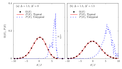
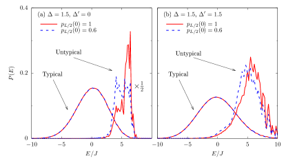
In Fig. 9, the DOS of $\mathcal{H}$ with $L=24$ sites is shown for both, an integrable ($\Delta=1.5$, $\Delta^{\prime}=0$) and a non-integrable ($\Delta=\Delta^{\prime}=1.5$) case. Note that $L=24$ is sufficient to capture the overall shape of the DOS. In both cases, $\Omega(E)$ has a broad Gaussian-like shape jin2016 . In addition, the LDOS $P(E)$ is shown for a typical state with random coefficients $c_{k}$ and an untypical state where all $c_{k}$ are the same. For the typical state, $P(E)$ apparently coincides with the DOS of $\mathcal{H}$. This fact also reflects that a typical state imitates the high-temperature statistical ensemble. In contrast, for an untypical state, $P(E)$ is sharply peaked at the upper border of the spectrum. This fact clearly shows that an untypical state does not imitate the high-temperature statistical ensemble. Moreover, since in the gapped phase $\Delta>1$ the dynamics at the spectral border is expected to be insulating, this fact provides a reasonable explanation for the frozen density profiles in Fig. 8 (a).

Figure 9: (Color online) Density of states $\Omega(E)$ of $\mathcal{H}$ with $L=24$ sites and local density of states $P(E)$ for states with random $c_{k}$ and equal $c_{k}$. Other parameters: (a) $\Delta=1.5$, $\Delta^{\prime}=0$; (b) $\Delta=\Delta^{\prime}=1.5$.

VI.2 Internal randomness and entanglement

So far, we have only distinguished between typical states, which are completely random, and untypical states, where the coefficients $c_{k}$ are all equal. At this point, we also analyze the role of the amount of internal randomness. Moreover, we are interested in the influence of this randomness on the entanglement of our non-equilibrium states.

In order to measure the entanglement entropy schollwoeck2005 (EE) of a given state $\ket{\psi}$, we divide our system into a left part $A$ and a right part $B$ of equal size. Accordingly, we write $\ket{\psi}$ as

$$\ket{\psi}=\sum_{i=1}^{d_{A}}\sum_{j=1}^{d_{B}}\psi_{i,j}\ket{i}\otimes\ket{j}\ ,$$ (36)

where $d_{A}$, $d_{B}$ are the Hilbert-space dimensions of $A$, $B$ and $\{\ket{i}\}$, $\{\ket{j}\}$ are orthonormal product bases of $A$, $B$. The reduced density matrix $\rho_{A}$ of part A is then given by

$$\rho_{A}=\text{Tr}_{B}\ket{\psi}\bra{\psi}\ ,$$ (37)

where the states $\ket{j}$ from part $B$ are traced out,

$$\braket{i}{\rho_{A}}{i^{\prime}}=\sum_{j=1}^{d_{B}}\psi_{i,j}\,\psi_{i^{\prime},j}^{\ast}\ .$$ (38)

By construction, the reduced density matrix $\rho_{A}$ has $d_{A}$ eigenvalues $\omega_{\alpha}$ with $\sum_{\alpha}\omega_{\alpha}=1$. These eigenvalues are then used to compute the EE, which is defined as

$$S=-\text{Tr}[\rho_{A}\log_{2}\rho_{A}]=-\sum_{\alpha=1}^{d_{A}}\omega_{\alpha}\log_{2}\omega_{\alpha}\ .$$ (39)

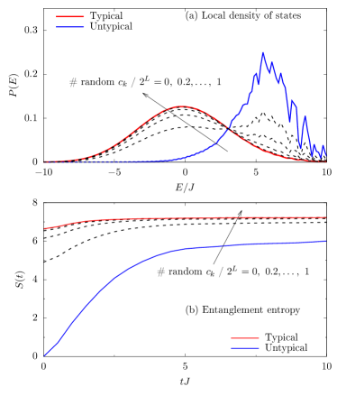
Before we discuss the EE below, the LDOS $P(E)$ is depicted in Figs. 10 (a) and (b) for states where the percentage of random coefficients $c_{k}$ is varied between $0\%$ and $100\%$. As before, $L=24$ sites are sufficient. First, one observes that $P(E)$ becomes continuously broader for increasing randomness. In fact, for approximately $60\%$ random coefficients, $P(E)$ already has a pronounced Gaussian shape and is almost identical to the LDOS of a completely random state or the DOS $\Omega(E)$ of the Hamiltonian.

In Fig. 10 (b) the corresponding EE is now depicted for $L=16$ sites, as obtained from ED. One observes that $S(t)$ monotonically increases at short times, until it eventually turns into a plateau with $S(t)\approx\text{const}$. Moreover, this saturation value increases with the number of random coefficients $c_{k}$ Page1993 . For an untypical state, where all $c_{k}$ are the same, we see that $S(0)=0$, which confirms that $\ket{\psi}$ can be written as a product state [cf. Eq. (7)].

Comparing Figs. 10 (a) and (b), it is evident that for our non-equilibrium states either a broad LDOS and high EE or a narrow LDOS and low EE occur simultaneously. Thus, low EE could be another explanation for the dynamics observed in in Fig. 8. This possibility is examined below. Note that the anisotropies in Fig. 10 have been set to $\Delta=\Delta^{\prime}=1.5$. We have checked, however, that the qualitative behavior of $P(E)$ and $S(t)$ is independent of the specific choice of $\Delta$ and $\Delta^{\prime}$ and system size $L$.

Figure 10: (Color online) (a) Local density of states $P(E)$ for states with a different number of random coefficients $c_{k}$ for a chain with $L=24$ sites. (b) Corresponding entanglement entropy $S(t)$ for a system with $L=16$ sites. In both cases, we have $\Delta=\Delta^{\prime}=1.5$.

VI.3 Random product state

As a final test to what extend internal randomness, entanglement, and LDOS influence the real-time dynamics of our initial states, we now define a convenient state

$$\ket{\psi_{P}}=\sum_{ij}c_{ij}\ket{i}\otimes\ket{\uparrow}\otimes\ket{j}\ ,$$ (40)

where $c_{ij}=c_{i}c_{j}$ are complex coefficients and the sum runs over all states $\ket{i}$ and $\ket{j}$ of the left and right half of the chain respectively. By construction, $\ket{\psi_{P}}$ is a product state and the initial density profile is identical to the class of states defined in Eq. (6). Concerning the internal randomness, however, the construction of $\ket{\psi_{P}}$ only involves $\sim 2^{L/2}$ random numbers, which is considerably less compared to a typical state with $2^{L}$ independent random coefficients.

Figure 11: (Color online) (a) Comparison of density profiles $p_{l}(t)$ for a typical state [see Eq. (6)] and a product state $\ket{\psi_{P}}$ [see Eq. (40)] at fixed times $tJ=5$ and $10$. (b) Local density of states $P(E)$ of these states for a chain with $L=24$ sites. (c) Corresponding entanglement entropy $S(t)$ for a system with $L=16$ sites. In all cases, we have $\Delta=1.5$ and $\Delta^{\prime}=0$.

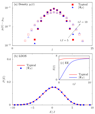
In Fig. 11 (a), the density profiles $p_{l}(t)$ of a typical state and a state $\ket{\psi_{P}}$ according to Eq. (40) are depicted for fixed times $tJ=5$ and $10$. We restrict ourselves to the integrable case with $\Delta=1.5$, $\Delta^{\prime}=0$ and $L=26$ sites. In order to minimize the dependence on the specific random initialization, the data for $\ket{\psi_{P}}$ is averaged over $N=20$ different initial states. Note, however, that the total amount of random coefficients, $\sim 20\cdot 2^{L/2}$, is still much smaller than $2^{L}$. The semi-log plot in Fig. 11(a) illustrates that the differences between a typical state and $\ket{\psi_{P}}$ are hardly visible for all times shown here.

In Fig. 11 (b), the corresponding LDOS of both states is shown. One observes that $\ket{\psi_{P}}$ has a broad spectral distribution with a Gaussian shape which very close to the LDOS of the typical state. In Fig. 11 (c), we also show the entanglement entropy of both states. At $t=0$, $S(t)$ vanishes for $\ket{\psi_{P}}$ by construction. However, at longer times, $S(t)$ saturates at the same value as the typical state. These results suggest that the lack of initial entanglement is not the origin of the untypical dynamics observed in Fig. 8.

VII Conclusion

To summarize, we have investigated the real-time broadening of non-equilibrium density profiles and, in particular, the role of the specific initial-state realization in non-integrable systems. To this end, we have focused on a particular class of initial states. This class consists of pure states and features initial density profiles with a pronounced peak on top of a homogeneous many-particle background at any temperature. As a first step, however, we have concentrated on the limit of high temperatures. Since this particular class of initial states allows for changing internal degrees of freedom without modifying the initial density profile, a central question has been whether and in how far such internal details influence the real-time and real-space dynamics. In this context, typicality of pure states is an useful concept and implies for internal randomness a dynamical behavior in agreement with the equilibrium correlation function. Still, this concept does not predict the type of transport as such and cannot be applied to initial states without any randomness. In particular, it cannot answer whether and for which initial conditions diffusion occurs in isolated systems.

As an example of a non-integrable system, we have studied the XXZ spin-$1/2$ chain, where integrability is broken due to a next-nearest neighbor interaction. Using large-scale numerical simulations, we have first unveiled that random initial states yield diffusive broadening in the regime of strong interactions. Quite remarkably, in this regime, we have found that signatures of diffusion are equally pronounced for the non-integrable and integrable model. Our numerical simulations in real space, as well as a Fourier analysis, have further shown the existence of diffusion for weaker interactions, as long as integrability is broken.

Finally, since we have observed that non-random states can lead to entirely different behavior, we have characterized typical and untypical states in terms of the amount of internal randomness, the local density of states, and the entanglement entropy. Here, our numerical results have suggested that different initial conditions lead to the same dynamical behavior if their local density of states is similar. The initial entanglement entropy, on the other hand, does not seem to be a crucial property. The latter we have demonstrated for a random product state.

Promising future research directions include the study of real-time dynamics of typical and untypical states in a wider class of non-integrable systems, e.g., in extended Hubbard models or spin models with disorder, also at lower temperatures. In addition to transport of spin and charge, it would also be interesting to investigate energy dynamics as well.

Appendix A Influence of initial peak height

In the main text, we have focused on initial states $\ket{\psi(0)}$ with the maximum amplitude $p_{L/2}(0)=1$ possible. For completeness, let us also discuss here whether or not the non-equilibrium dynamics depends on this particular choice. By choosing $a>0$ in the definition of our initial states [see Eq. (6)], it is possible to construct states with $p_{L/2}(0)<1$, which are in this sense closer to equilibrium. Note that $p_{l\neq L/2}(0)=p_{\text{eq}}=1/2$ is unaffected by $a>0$.

First, it is instructive to show how the size of the initial peak $p_{L/2}(0)$ in the middle of the chain is controlled by the parameter $a$. To this end, the following calculation can be performed.

$$\frac{\bra{\psi}n_{L/2}\ket{\psi}}{\braket{\psi}{\psi}} =\frac{\bra{(n_{L/2}-a)\Phi}n_{L/2}\ket{(n_{L/2}-a)\Phi}}{\braket{(n_{L/2}-a)\Phi}{(n_{L/2}-a)\Phi}}$$ (41)

$$=\frac{\bra{\Phi}(n_{L/2}-a)n_{L/2}(n_{L/2}-a)\ket{\Phi}}{\bra{\Phi}(n_{L/2}-a)(n_{L/2}-a)\ket{\Phi}}$$ (42)

$$=\frac{(1-a)^{2}\bra{\Phi}n_{L/2}\ket{\Phi}}{(1-2a)\bra{\Phi}n_{L/2}\ket{\Phi}+a^{2}\braket{\Phi}{\Phi}}$$ (43)

In the last step, we have multiplied out brackets and used the projection property $n_{L/2}^{3}=n_{L/2}^{2}=n_{L/2}$. Since $\bra{\Phi}n_{L/2}\ket{\Phi}=\braket{\Phi}{\Phi}/2$, one therefore finds that $p_{L/2}(0)$ does not depend linearly on $a$ but rather follows

$$p_{L/2}(0)=\frac{\bra{\psi}n_{L/2}\ket{\psi}}{\braket{\psi}{\psi}}=\frac{(1-a)^{2}}{(1-a)^{2}+a^{2}}\ .$$ (44)

It follows that for $a=0$ we have $p_{L/2}(0)=1$, whereas for $a=0.5$ we have $p_{L/2}(0)=p_{\text{eq}}=0.5$.

Figure 12: (Color online) Density profile $p_{l}(t)$ for untypical initial states with $p_{L/2}(0)=1$ and $p_{L/2}(0)=0.6$ at fixed times $tJ=5$ (filled symbols), $tJ=10$ (open symbols) for a chain with $L=26$ sites and different anisotropies: (a) $\Delta=1.5$, $\Delta^{\prime}=0$; (b) $\Delta=1.5$, $\Delta^{\prime}=1.5$. For a meaningful comparison, the data for $p_{L/2}(0)=0.6$ is multiplied by a factor $5$.

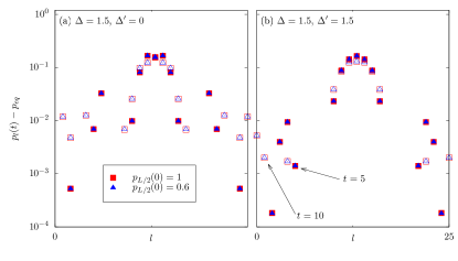
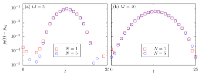
We now present the simulation results. Here, we focus on the case of untypical states, i.e., all $c_{k}$ are equal, and compare the dynamics of a state with $p_{L/2}(0)=1$ and a state with $p_{L/2}(0)=0.6$. In Fig. 12, the resulting density profiles $p_{l}(t)$ are shown for $L=26$ and different anisotropies $\Delta$, $\Delta^{\prime}$, at fixed times $tJ=5$, $10$. For a meaningful comparison, the data for $p_{L/2}(0)=0.6$ is multiplied remark by an overall scaling factor $5$. Remarkably, after this simple renormalization, the data for $p_{L/2}(0)=1$ and $p_{L/2}(0)=0.6$ exactly coincide with each other.

This illustrates that for an untypical state the dynamics of $p_{l}(t)$ is independent of the specific initial value $p_{L/2}(0)$. In particular, by changing the parameter $a>0$, it is not possible to change the dynamical behavior of untypical states depicted in Fig. 8 in the main text of this paper. Although not shown here explicitly, we have found that this independence of the parameter $a$ applies to typical states as well. Note that this independence can be also understood analytically for so-called binary operators richter2017 .

Finally, let us comment on the influence of $a>0$ on the LDOS $P(E)$. In Fig. 13, we show $P(E)$ for typical as well as untypical initial states and compare the case of maximum amplitude $p_{L/2}(0)=1$ to the case of $p_{L/2}(0)=0.6$. One observes that, although the spectral weight is slightly redistributed compared to the case of $a=0$, $P(E)$ is almost unaffected by a nonzero parameter $a>0$. Thus, irrespective of the initial amplitude $p_{L/2}(0)$, a typical state has a broad Gaussian LDOS, whereas an untypical state goes along with a narrow LDOS at the upper border of the spectrum.

Figure 13: (Color online) Local density of states $P(E)$ for typical and untypical states with $p_{L/2}(0)=1$ (solid lines) and $p_{L/2}(0)=0.6$ (dashed lines). We use $L=24$ in both cases. Other parameters: (a) $\Delta=1.5$, $\Delta^{\prime}=0$; (b) $\Delta=\Delta^{\prime}=1.5$.

Appendix B Dynamics for small anisotropies

In the main part of this paper, we found that the non-equilibrium dynamics of of $p_{l}(t)$ is diffusive in the regime of strong anisotropies $\Delta$ and $\Delta^{\prime}$, irrespective of the model being integrable or non-integrable. Furthermore, we argued that diffusion also emerges for smaller anisotropies, as long as integrability is broken, i.e. $\Delta^{\prime}>0$.

Let us briefly comment on the regime of small interactions $\Delta,\Delta^{\prime}<1$. In Fig. 14, the generalized diffusion coefficient $D_{q}(t)$, as obtained from the non-equilibrium dynamics, is shown for momenta $k=q/(2\pi/L)=1,\ 2$ and anisotropies $\Delta=0.5$, $\Delta^{\prime}=0$ as well as $\Delta=0.5$, $\Delta^{\prime}=0.5$. For comparison, we also depict the diffusion coefficient $D_{q=0}(t)$, i.e. calculated from LRT. Concerning the non-integrable model in Fig. 14 (b) we observe that for $q=0$, $D(t)$ eventually reaches a constant plateau at times $tJ\sim 20$. However, we are unable to find such a time-independent regime for any $q\neq 0$. Nevertheless, we argue that these results by no means rule out the possibility of diffusion. In fact, it turns out that in this parameter regime, the mean free time as well as the corresponding mean free path, are too long to draw reliable conclusion. Thus, although our data provides no clear evidence, they strongly suggest the emergence of diffusion in the thermodynamic limit also in the regime of weak interactions, as long as $\Delta^{\prime}>0$. This conclusion is further supported by the comparison with the integrable case, as shown in Fig. 14 (a). Here, transport is clearly ballistic, $D(t)\propto t$, and at least for $k=0$ and $k=1$, there are distinct differences between the integrable and the non-integrable model.

Figure 14: (Color online) Generalized diffusion coefficient $D_{q}(t)$, obtained from the non-equilibrium density profiles according to Eq. (21) for momenta $q/(2\pi/L)=k$, $L=36$. As a comparison, $D_{q=0}(t)$ according to LRT is shown for $L=33$. Moreover, we also depict data obtained by perturbation theory (PT) steinigeweg2011_2 . Other parameters: (a) $\Delta=0.5$, $\Delta^{\prime}=0$. (b) $\Delta=0.5$, $\Delta^{\prime}=0.5$.

Appendix C Averaging over initial states

We briefly discuss the accuracy of our pure-state approach. For a typical initial state, the real and imaginary part of the coefficients $c_{k}$ are drawn randomly from a Gaussian distribution with zero mean. Therefore, the resulting dynamics naturally depends on the specific realization of these random numbers. In order to reduce this dependence, we may average over $N>1$ different initializations.

In Fig. 15, the density profile $p_{l}(t)$ is depicted for fixed times $tJ=5$, $10$ for a chain with $L=26$ sites and anisotropies $\Delta=1.5$, $\Delta^{\prime}=0$. Data for $N=1$ random state are compared to data which is obtained by averaging over $N=5$ random configurations. While the Gaussian shape is already visible for $N=1$, deviations from this Gaussian form at the boundaries are slightly reduced for the averaged data. However, these differences are very small and do not influence the general result. It is therefore sufficient to only consider $N=1$, as done throughout the main text of this paper. We note that, according to typicality, errors decrease exponentially with increasing system size such that averaging becomes even less important for our large systems with $L=36$ sites.

Figure 15: (Color online) Density profile $p_{l}(t)$ with respect to site $l$ at fixed times $tJ=5,\ 10$ for the integrable case $\Delta=1.5$, $\Delta^{\prime}=0$ and system size $L=26$, shown in a semi-log plot. Data for $N=1$ random state are compared to data averaged over $N=5$ random states.

Appendix D Forward propagation in real time

In order to perform a forward propagation of pure states in real time, we employ two different methods, i.e., a fourth-order Runge-Kutta (RK4) scheme for medium systems ($L\leq 26$) as well as a Trotter product formula for large systems ($L>26$). Here, we briefly summarize the working principle of both methods.

The time-dependent Schrödinger equation reads

$$i\partial_{t}\ket{\psi(t)}=\mathcal{H}\ket{\psi(t)}\ ,$$ (45)

where $\hbar=1$ is set to unity. It is formally solved by

$$\ket{\psi(t^{\prime})}=U(t,t^{\prime})\ket{\psi(t)}\ ,$$ (46)

with $U(t,t^{\prime})=e^{-i\mathcal{H}(t^{\prime}-t)}$. While the exact evaluation of Eq. (46) requires diagonalization of $\mathcal{H}$, we here use accurate approximations of the time-evolution operator $U(t,t^{\prime})$.

Within the RK4 method, the Schrödinger equation is iteratively solved according to

$$\ket{\psi(t+\delta t)}=\ket{\psi(t)}+\ket{\psi_{1}}+\ket{\psi_{2}}+\ket{\psi_{3}}+\ket{\psi_{4}}\ ,$$ (47)

where the $\ket{\psi_{k}}$ are computed as follows: $\ket{\psi_{k}}=(-i\mathcal{H})^{k}\delta t^{k}\ket{\psi(t)}/k!$. In order to ensure small numerical errors, we use a short time step $\delta tJ=0.01\ll 1$ steinigeweg2014 ; steinigeweg2015 ; steinigeweg2016 .

Concerning the Trotter product-formula, we use a second-order approximation of the time-evolution operator $U(t,t+\delta t)=U(\delta t)$, given by

$$\widetilde{U}_{2}(\delta t)=e^{-i\frac{\delta t}{2}{\cal H}_{k}}\cdots e^{-i\frac{\delta t}{2}{\cal H}_{1}}e^{-i\frac{\delta t}{2}{\cal H}_{1}}\cdots e^{-i\frac{\delta t}{2}{\cal H}_{k}}\,,$$ (48)

where ${\cal H}={\cal H}_{1}+\cdots+{\cal H}_{k}$. The approximation is bounded by

$$||U(\delta t)-\widetilde{U}_{2}(\delta t)||\ll c_{2}\,\delta t^{3}\,,$$ (49)

where $c_{2}$ is a positive constant.

In practice, we use an XYZ decomposition for the Hamiltonian according to the $x$, $y$, and $z$ components of the spin operators, i.e., ${\cal H}={\cal H}_{x}+{\cal H}_{y}+{\cal H}_{z}$. The computational basis states are eigenstates of the $S^{z}$ operators. Thus, in this representation $e^{-i\delta t{\cal H}_{z}}$ is diagonal by construction, and it only changes the input state by altering the phase of each of the basis vectors. By an efficient basis rotation into the eigenstates of the $S^{x}$ or $S^{y}$ operators, the operators $e^{-i\delta t{\cal H}_{x}}$ and $e^{-i\delta t{\cal H}_{y}}$ act as $e^{-i\delta t{\cal H}_{z}}$.

Appendix E Calculation of DOS and LDOS

As discussed in the main part of this paper, it is possible to compute the (local) density of states by exact diagonalization. In this paper, however, we have relied on an alternative numerical approach to the DOS and LDOS hams2000 ; jin2016 . Again, we exploit the forward propagation of pure states in real time. The DOS can be written as

$$\Omega(E) =\sum_{n}\delta(E-E_{n})\ ,$$ (50)

$$=\frac{1}{2\pi}\int\limits_{-\infty}^{\infty}e^{itE}\ \text{Tr}[e^{-i\mathcal{H}t}]\,\text{d}t\ ,$$ (51)

where we have used the definition of the $\delta$ function. According to the principle of typicality, the trace in Eq. (50) can be evaluated by

$$\text{Tr}[e^{-i\mathcal{H}t}]\approx\bra{\Phi(0)}e^{-i\mathcal{H}t}\ket{\Phi(0)}=\braket{\Phi(0)}{\Phi(t)}\ ,$$ (52)

with a randomly drawn state $\ket{\Phi}$. Consequently, the DOS can approximately be written as

$$\Omega(E)\approx C\int_{-\Theta}^{+\Theta}e^{itE}\braket{\Phi(0)}{\Phi(t)}\text{d}t\ ,$$ (53)

with $\braket{\Phi(0)}{\Phi(-t)}=\braket{\Phi(0)}{\Phi(t)}^{\ast}$ and some normalization constant $C$. The energy resolution is given by $\Delta E=\pi/\Theta$. Similarly, it is possible to define the LDOS $P(E)$ of a state $\ket{\psi}$ according to

$$P(E) =\sum_{n}|\braket{n}{\psi}|^{2}\,\delta(E-E_{n})$$ (54)

$$=\frac{1}{2\pi}\int_{-\infty}^{\infty}e^{itE}\bra{\psi}e^{-it\mathcal{H}}\ket{\psi}\text{d}t$$ (55)

$$\approx C\int_{-\Theta}^{+\Theta}e^{itE}\bra{\psi}e^{-it\mathcal{H}}\ket{\psi}\text{d}t\ \ .$$ (56)

Note that the concept of typicality is not needed in Eqs. (55) and (56).

Since the above Fourier transforms of, e.g., $\braket{\psi}{\psi(t)}$ formally require a signal from $t=-\infty$ to $t=\infty$, the approximation by Eq. (56) with finite times $\Theta<\infty$ might lead to certain complications. This is in particular the case if the spectral representation of $\ket{\psi}$ is very sparse, i.e., if many coefficients $|\braket{n}{\psi}|^{2}$ are zero. Then, the function $\braket{\psi}{\psi(t)}$ does not necessarily decay, but can rather exhibit strong, almost periodic oscillations. As a consequence, the finite-time Fourier transform of such a signal is usually no smooth function, especially in the case of a high-frequency resolution, i.e., in the case of large cut-off time $\Theta$.

A common approach to account at least partially for this problem is the convolution of $\braket{\psi}{\psi(t)}$ with a suitable window function. This window function, e.g., a Gaussian, introduces a damping of $\braket{\psi}{\psi(t)}$ at long times and thus leads to a well-behaved Fourier transform. In the present paper, however, we refrain from using any kind of such artificial line broadening. In cases where $\braket{\psi}{\psi(t)}$ is not decaying on a reasonable time scale, we simply restrict ourselves to short cutoff times $\Theta J\approx 20$, giving rise to a coarse energy resolution of about $\delta E/J\approx 0.15$. The resulting Fourier transform therefore does not necessarily produce the exact LDOS, but rather shows the general shape of $P(E)$. Since our aim is only to make qualitative statements about the basic behavior of $P(E)$, this procedure is adequate.

References

- (1) A. Polkovnikov, K. Sengupta, A. Silva, and M. Vengalattore, Rev. Mod. Phys.83, 863 (2011).
- (2) J. Eisert, M. Friesdorf, and C. Gogolin, Nature Phys. 11, 124 (2015).
- (3) I. Bloch, Science 319, 1202 (2008).
- (4) T. Langen, R. Geiger, and J. Schmiedmayer, Annu. Rev. Condens. Matter Phys. 6, 201 (2015).
- (5) D. M. Basko, I. L. Aleiner, and B. L. Altshuler, Ann. Phys. 321, 1126 (2006).
- (6) R. Nandkishore and D. A. Huse, Annu. Rev. Condens. Matter Phys. 6, 15 (2015).
- (7) D. A. Abanin and Z. Papić, Ann. Phys. 529, 1700169 (2017).
- (8) U. Schollwöck, Rev. Mod. Phys. 77, 259 (2005).
- (9) U. Schollwöck, Ann. Phys. 326, 96 (2011).
- (10) S. Goldstein, J. L. Lebowitz, R. Tumulka, and N. Zanghì, Phys. Rev. Lett. 96, 050403 (2006).
- (11) S. Popescu, A. J. Short, and A. Winter, Nat. Phys. 2, 754 (2006).
- (12) P. Reimann, Phys. Rev. Lett. 99, 160404 (2007).
- (13) J. Gemmer and G. Mahler, Eur. Phys. J. B 31, 249 (2003).
- (14) S. Sugiura, and A. Shimizu, Phys. Rev. Lett. 108, 240401 (2012).
- (15) S. Sugiura and A. Shimizu, Phys. Rev. Lett. 111, 010401 (2013).
- (16) T. A. Elsayed and B. V. Fine, Phys. Rev. Lett. 110, 070404 (2013).
- (17) T. Iitaka and T. Ebisuzaki, Phys. Rev. Lett. 90, 047203 (2003).
- (18) T. Iitaka and T. Ebisuzaki, Phys. Rev. E 69, 057701 (2004).
- (19) S. R. White, Phys. Rev. Lett. 102, 190601 (2009).
- (20) T. Monnai and A. Sugita, J. Phys. Soc. Jpn. 83, 094001 (2014).
- (21) P. Reimann, Nature Comm. 7, 10821 (2016).
- (22) J. M. Deutsch, Phys. Rev. A 43, 2046 (1991).
- (23) M. Srednicki, Phys. Rev. E 50, 888 (1994).
- (24) M. Rigol, V. Dunjko, and M. Olshanii, Nature 452, 854 (2008).
- (25) P. Reimann, Phys. Rev. Lett. 101, 190403 (2008).
- (26) L. D’Alessio, Y. Kafri, A. Polkovnikov, and M. Rigol, Adv. Phys. 65, 239 (2016).
- (27) F. Bonetto, J. L. Lebowitz, and L. Rey-Bellet, Fourier’s law: A challenge to theorists in Mathematical physics 2000 (World Scientific Publishing Company, Singapore, 2000).
- (28) M. Buchanan, Nature Phys. 1, 71 (2005).
- (29) B. S. Shastry, Phys. Rev. Lett. 56, 1529 (1986).
- (30) X. Zotos, F. Naef, and P. Prelovšek, Phys. Rev. B 55, 11029 (1997).
- (31) T. Prosen, Phys. Rev. Lett. 106, 217206 (2011).
- (32) T. Prosen and E. Ilievski, Phys. Rev. Lett. 111, 057203 (2013).
- (33) E. Ilievski, M. Medenjak, T. Prosen, and L. Zadnik, J. Stat. Mech. 2016, 064008 (2016).
- (34) F. H. L. Essler and M. Fagotti, J. Stat. Mech. 2016, 064002 (2016).
- (35) L. Vidmar and R. Rigol, J. Stat. Mech. 2016, 064007 (2016).
- (36) R. Vasseur and J. E. Moore, J. Stat. Mech. 2016, 064010 (2016).
- (37) X. Zotos and P. Prelovšek, Transport in One-Dimensional Quantum Systems in Strong Interactions in Low Dimensions (Kluwer Academic Publishers, Dordrecht, 2004).
- (38) F. Heidrich-Meisner, A. Honecker, D. C. Cabra, and W. Brenig, Phys. Rev. B 68, 134436 (2003).
- (39) F. Heidrich-Meisner, A. Honecker, and W. Brenig, Eur. Phys. J. Special Topics 151, 135 (2007).
- (40) M. Žnidarič, Phys. Rev. Lett. 106, 220601 (2011).
- (41) R. Steinigeweg and W. Brenig, Phys. Rev. Lett. 107, 250602 (2011).
- (42) C. Karrasch, J. E. Moore, and F. Heidrich-Meisner, Phys. Rev. B 89, 075139 (2014).
- (43) R. Steinigeweg, F. Jin, D. Schmidtke, H. de Raedt, K. Michielsen, and J. Gemmer, Phys. Rev. B 95, 035155 (2017).
- (44) T. Prosen and M. Žnidarič, Phys. Rev. B 86, 125118 (2012).
- (45) C. Karrasch, T. Prosen, and F. Heidrich-Meisner, Phys. Rev. B 95, 060406(R) (2017).
- (46) R. Steinigeweg, F. Jin, H. De Raedt, K. Michielsen, and J. Gemmer, Phys. Rev. E 96, 020105(R) (2017).
- (47) A. Klümper and K. Sakai, J. Phys. A 35, 2173 (2002).
- (48) L. F. Santos, J. Phys. A 37, 4723 (2004).
- (49) L. F. Santos and M. Rigol, Phys. Rev. E 81, 036206 (2010).
- (50) C. Bartsch and J. Gemmer, Phys. Rev. Lett. 102, 110403 (2009).
- (51) C. Bartsch and J. Gemmer, EPL (Europhys. Lett.) 96, 60008 (2011).
- (52) R. Kubo, J. Phys. Soc. Jpn. 12, 570 (1957).
- (53) J. M. Luttinger, Phys. Rev. 135, A1505 (1964).
- (54) G. D. Mahan, Many-Particle Physics (Plenum Press, New York, London, 1990).
- (55) C. Karrasch, J. H. Bardarson, and J. E. Moore, Phys. Rev. Lett. 108, 227206 (2012).
- (56) C. Karrasch, J. Hauschild, S. Langer, and F. Heidrich-Meisner, Phys. Rev. B 87, 245128 (2013).
- (57) R. Steinigeweg, J. Gemmer, and W. Brenig, Phys. Rev. Lett. 112, 120601 (2014).
- (58) R. Steinigeweg and J. Gemmer, Phys. Rev. B 80, 184402 (2009).
- (59) C. Karrasch, D. M. Kennes, and J. E. Moore, Phys. Rev. B 90, 155104 (2014).
- (60) R. Steinigeweg, J. Gemmer, and W. Brenig, Phys. Rev. B 91, 104404 (2015).
- (61) P. Prelovšek, S. El Shawish, X. Zotos, and M. Long, Phys. Rev. B 70, 205129 (2004).
- (62) M. Michel, G. Mahler, and J. Gemmer, Phys. Rev. Lett. 95, 180602 (2005).
- (63) R. Steinigeweg, H.-P. Breuer, and Jochen Gemmer, Phys. Rev. Lett. 99, 150601 (2007).
- (64) R. Steinigeweg, H. Wichterich, and J. Gemmer, EPL (Europhys. Lett.) 88, 10004 (2009).
- (65) Y. Yan, F. Jiang, and H. Zhao, Eur. Phys. J. B 88, 11 (2015).
- (66) D. J. Luitz and Y. B. Lev, Ann. Phys. 529, 1600350 (2017).
- (67) B. S. Shastry and B. Sutherland, Phys. Rev. Lett. 65, 243 (1990).
- (68) H. Castella, X. Zotos, and P. Prelovsek, Phys. Rev. Lett. 74, 972 (1995).
- (69) B. N. Narozhny, A. J. Millis, and N. Andrei, Phys. Rev. B 58, R2921 (1998).
- (70) X. Zotos, Phys. Rev. Lett. 82, 1764 (1999).
- (71) J. Benz, T. Fukui, A. Klümper, and C. Scheeren, J. Phys. Soc. Jpn. 74, 181 (2005).
- (72) S. Fujimoto and N. Kawakami, Phys. Rev. Lett. 90, 197202 (2003).
- (73) J. Herbrych, P. Prelovšek, and X. Zotos, Phys. Rev. B 84, 155125 (2011).
- (74) E. Ilievski and J. De Nardis, Phys. Rev. Lett. 119, 020602 (2017).
- (75) R. Steinigeweg, J. Herbrych, X. Zotos, and W. Brenig, Phys. Rev. Lett. 116, 017202 (2016).
- (76) A. Weiße, G. Wellein, A. Alvermann, and H. Fehske, Rev. Mod. Phys. 78, 275 (2006).
- (77) V. V. Dobrovitski and H. De Raedt, Phys. Rev. E 67, 056702 (2003).
- (78) H. De Raedt and K. Michielsen, in Handbook of Theoretical and Computational Nanotechnology (American Scientific Publishers, Los Angeles, 2006).
- (79) R. Steinigeweg, Phys. Rev. E 84, 011136 (2011).
- (80) R. Steinigeweg, EPL (Europhys. Lett.) 97, 67001 (2012).
- (81) M. Ljubotina, M. Žnidarič, and T. Prosen, Nature Comm. 8, 16117 (2017).
- (82) I. Khait, S. Gazit, N. Y. Yao, and A. Auerbach, Phys. Rev. B 93, 224205 (2016).
- (83) J. Sirker, R. G. Pereira, and I. Affleck, Phys. Rev. Lett. 103, 216602 (2009).
- (84) J. Sirker, R. G. Pereira, and I. Affleck, Phys. Rev. B 83, 035115 (2011).
- (85) S. Grossjohann and W. Brenig, Phys. Rev. B 81, 012404 (2010).
- (86) D. Gobert, C. Kollath, U. Schollwöck, and G. Schütz, Phys. Rev. E 71, 036102 (2005).
- (87) A. Hams and H. De Raedt, Phys. Rev. E 62, 4365 (2000).
- (88) F. Jin, R. Steinigeweg, H. De Raedt, K. Michielsen, M. Campisi, and J. Gemmer, Phys. Rev. E 94, 012125 (2016).
- (89) D. N. Page, Phys. Rev. Lett. 71, 1291 (1993).
- (90) M. Stephan and J. Docter, J. Large-Scale Res. Facil. A1, 1 (2015).
- (91) J. Richter and R. Steinigeweg, arXiv:1711.00672 (2017).
- (92) The factor 5 compensates the fact that for , we have , whereas for , we have .