A unified framework for asymptotic analysis and computation of finite Hankel transform

Abstract

In this paper we present a unified framework for asymptotic analysis and computation of the finite Hankel transform. This framework enables us to derive asymptotic expansions of the transform, including the cases where the oscillator has zeros and stationary points. As a consequence, two efficient and affordable methods for computing the transform numerically are developed and a detailed analysis of their asymptotic error estimate is carried out. Numerical examples are provided to confirm our analysis.

Keywords: finite Hankel transform, oscillatory integrals, asymptotic expansion.

Mathematics Subject Classification 65D30, 65D32, 65R10, 41A60.

1 Introduction

The finite Hankel transform of a function $f:[a,b]\rightarrow\mathbb{R}$ with a general oscillator $g$ is defined by

$$\mathcal{H}_{\nu}[f]:=\int_{a}^{b}f(x)J_{\nu}(\omega g(x))dx,$$ (1.1)

where $J_{\nu}(x)$ is the Bessel function of the first kind of order $\nu$ and $\omega>0$ is a large parameter. This transform plays an important role in many physical problems such as boundary value problems formulated in cylindrical coordinate [24], time dependent Schrödinger equation [4], electromagnetic scattering [3] and geometrical acoustics [5].

Closed forms for the finite Hankel transform are rarely available in general and, except in a few special cases, numerical methods are required to evaluate the transform accurately. However, the calculation with traditional quadrature rules may be prohibitively expensive due to the oscillatory character of the Bessel function. Roughly speaking, when $\omega\gg 1$, a fixed number of quadrature nodes per oscillation is required to obtain an acceptable level of accuracy, which makes the complexity grows linearly with $\omega$.

In the past decade, the evaluation of highly oscillatory integrals has been received considerable attention. In particular, for Fourier-type integrals of the form

$$\int_{a}^{b}f(x)e^{i\omega g(x)}dx,$$ (1.2)

several efficient methods such as asymptotic method [15, 16], Filon-type methods [15, 16, 29], Levin-type methods [17, 21], numerical steepest descent methods [8, 14], complex Gaussian quadrature [1, 2] and their different combinations or adaptive methods [10, 11, 13, 35] have been developed to compute the value of (1.2) with low computational cost. Among these methods, asymptotic method plays a fundamental role in clarifying these critical points, e.g., endpoints and stationary points, to the value of the integral and serves as a starting point of designing other efficient methods. We refer to the recent monograph [9] for a comprehensive survey.

In recent years, there has been a growing interest in studying numerical quadrature of the finite Hankel transform (1.1); see, for instance, [6, 7, 18, 22, 23, 27, 30, 31, 32, 34]. All these works focus on the simplest oscillator $g(x)=x$ and asymptotic analysis has been carried out either by using the following differential equation [22, 32]

$$\mathbf{w}{{}^{\prime}}(x)=\mathbf{A}(\omega,x)\mathbf{w}(x),$$ (1.3)

where

$$\mathbf{w}(x)=\binom{J_{\nu-1}(\omega x)}{J_{\nu}(\omega x)},\quad\mathbf{A}(\omega,x)=\left(\begin{array}[]{cc}\frac{\nu-1}{x}&-\omega\\ \omega&-\frac{\nu}{x}\\ \end{array}\right),$$

or by using the well-known identity [28, 33]

$$\frac{d}{dz}(z^{\nu+1}J_{\nu+1}(z))=z^{\nu+1}J_{\nu}(z),\quad z,\nu\in\mathbb{C}.$$ (1.4)

For the Hankel transform with a general oscillator $g(x)$, very few studies have been conducted so far in the literature, except in the very special case where $g^{(j)}(a)=0$ for $j=0,\ldots,r$ and $r$ is some positive integer [33].

In this work, we aim to provide a complete asymptotic analysis and the construction of affordable quadrature rules for the finite Hankel transform with a general oscillator. Intuitively speaking, the main contribution to the value of the transform comes from the following three types of critical points:

1. Endpoints of the interval of integration, i.e., $x=a$ and $x=b$;

2. Zeros of the oscillator $\xi\in[a,b]$ where $g(\xi)=0$;

3. Stationary points of the oscillator $\zeta\in[a,b]$ where $g{{}^{\prime}}(\zeta)=0$.

For each type of critical point listed above, we will explore the asymptotic expansion of the transform. Note that the asymptotic analysis based on (1.3) fails when the oscillator $g(x)$ has zeros or stationary points on the integration interval. We will use the identity (1.4) and show that it is well suited for obtaining the asymptotic expansion of the finite Hankel transform. This is not trivial and requires more in-depth theoretical analysis. With these expansions in hand, we further develop two methods for computing the transform numerically and a rigorous analysis of their error is discussed.

The main results of the present paper can be summarized as follows:

• We provide a unified framework for asymptotic analysis of the finite Hankel transform. It enables us to obtain asymptotic expansions of the transform, especially in the presence of stationary points.

• Two methods for computing the transform are discussed and a detailed error analysis is performed. Compared to the method in [33], the method proposed here has the advantage of avoiding the use of diffeomorphism transformations which may be inconvenient in practice.

• We show that our analysis can be extended to the multivariate setting.

The structure of this paper is as follows. In the next section, we start with the ideal case where the oscillator $g(x)$ is free of stationary points, i.e., $g{{}^{\prime}}(x)\neq 0$ for $x\in[a,b]$. We distinguish our analysis into two cases according to $g(x)$ has a zero on $[a,b]$ or not. In addition, two methods for evaluating the transform numerically are developed and the behavior of their error is discussed thoroughly. In section 3 we deal with the case where $g(x)$ has a stationary point on the integration interval. The extension of our results is discussed in section 4 and some concluding remarks are presented in section 5.

Notation 1.1.

Throughout the paper, we denote the generalized moments of the Hankel transform $\mathcal{H}_{\nu}[f]$ by

$$M_{j}(\zeta,\nu,\omega)=\mathcal{H}_{\nu}[(x-\zeta)^{j}]=\int_{a}^{b}(x-\zeta)^{j}J_{\nu}(\omega g(x))dx,$$ (1.5)

where $\zeta\in[a,b]$ and $j\geq 0$. When $j=0$, note that $M_{0}(\zeta,\nu,\omega)$ does not depend on $\zeta$ anymore. Instead, we define $M(\nu,\omega)=M_{0}(\zeta,\nu,\omega)$.

2 The case with no stationary points

In this section we first consider the ideal case that the oscillator $g(x)$ has no stationary points in the integration interval $[a,b]$, i.e., $g{{}^{\prime}}(x)\neq 0$ for $x\in[a,b]$. We commence our analysis from the case that $g(x)\neq 0$ for $x\in[a,b]$.

2.1 The case $g(x)\neq 0$ for $x\in[a,b]$

We now state the first main result on the asymptotic expansion of $\mathcal{H}_{\nu}[f]$.

Theorem 2.1.

Let $f(x),g(x)\in C^{\infty}[a,b]$ and $g(x)\neq 0$, $g{{}^{\prime}}(x)\neq 0$ for $x\in[a,b]$. Then, for $\omega\rightarrow\infty$,

$$\mathcal{H}_{\nu}[f]\sim-\sum_{k=1}^{\infty}\frac{1}{(-\omega)^{k}}\left\{\frac{\sigma_{k-1}[f](b)}{g{{}^{\prime}}(b)}J_{\nu+k}(\omega g(b))-\frac{\sigma_{k-1}[f](a)}{g{{}^{\prime}}(a)}J_{\nu+k}(\omega g(a))\right\},$$ (2.1)

where $\sigma_{k}[f](x)$ are defined by

$$\sigma_{0}[f](x)=f(x),\quad\sigma_{k}[f](x)=g(x)^{\nu+k}\frac{d}{dx}\left[\frac{\sigma_{k-1}[f](x)}{g(x)^{\nu+k}g{{}^{\prime}}(x)}\right],\quad k\geq 1.$$ (2.2)

Proof.

We shall first prove by induction on $m$ the following identity

$$\mathcal{H}_{\nu}[f] =-\sum_{k=1}^{m}\frac{1}{(-\omega)^{k}}\left\{\frac{\sigma_{k-1}[f](b)}{g{{}^{\prime}}(b)}J_{\nu+k}(\omega g(b))-\frac{\sigma_{k-1}[f](a)}{g{{}^{\prime}}(a)}J_{\nu+k}(\omega g(a))\right\}$$

$$~{}~{}~{}~{}~{}~{}~{}~{}~{}~{}+\frac{1}{(-\omega)^{m}}\mathcal{H}_{\nu+m}[\sigma_{m}[f]].$$ (2.3)

When $m=0$, it is trivial. Now suppose (2.1) is true for $m$, we wish to prove it for $m+1$.

By taking $z=\omega g(x)$ and replacing $\nu$ by $\nu+m$ in (1.4), we obtain

$$\frac{d}{dx}\left[g(x)^{\nu+m+1}J_{\nu+m+1}(\omega g(x))\right]=\omega g{{}^{\prime}}(x)g(x)^{\nu+m+1}J_{\nu+m}(\omega g(x)).$$ (2.4)

Inserting this into $\mathcal{H}_{\nu+m}[\sigma_{m}[f]]$ and using integration by parts we find

$$\mathcal{H}_{\nu+m}[\sigma_{m}[f]] =\int_{a}^{b}\sigma_{m}[f](x)J_{\nu+m}(\omega g(x))dx$$

$$=\frac{1}{\omega}\int_{a}^{b}\frac{\sigma_{m}[f](x)}{g(x)^{\nu+m+1}g{{}^{\prime}}(x)}\frac{d}{dx}\left[g(x)^{\nu+m+1}J_{\nu+m+1}(\omega g(x))\right]dx$$

$$=\frac{1}{\omega}\left[\frac{\sigma_{m}[f](b)}{g{{}^{\prime}}(b)}J_{\nu+m+1}(\omega g(b))-\frac{\sigma_{m}[f](a)}{g{{}^{\prime}}(a)}J_{\nu+m+1}(\omega g(a))\right]$$

$$~{}~{}~{}~{}~{}~{}~{}-\frac{1}{\omega}\int_{a}^{b}g(x)^{\nu+m+1}\frac{d}{dx}\left[\frac{\sigma_{m}[f](x)}{g(x)^{\nu+m+1}g{{}^{\prime}}(x)}\right]J_{\nu+m+1}(\omega g(x))dx$$

$$=\frac{1}{\omega}\left[\frac{\sigma_{m}[f](b)}{g{{}^{\prime}}(b)}J_{\nu+m+1}(\omega g(b))-\frac{\sigma_{m}[f](a)}{g{{}^{\prime}}(a)}J_{\nu+m+1}(\omega g(a))\right]$$

$$~{}~{}~{}~{}~{}~{}~{}-\frac{1}{\omega}\mathcal{H}_{\nu+m+1}[\sigma_{m+1}[f]],$$

which, together with (2.1), implies that

$$\mathcal{H}_{\nu}[f] =-\sum_{k=1}^{m+1}\frac{1}{(-\omega)^{k}}\left\{\frac{\sigma_{k-1}[f](b)}{g{{}^{\prime}}(b)}J_{\nu+k}(\omega g(b))-\frac{\sigma_{k-1}[f](a)}{g{{}^{\prime}}(a)}J_{\nu+k}(\omega g(a))\right\}$$

$$~{}~{}~{}~{}~{}~{}~{}~{}~{}~{}+\frac{1}{(-\omega)^{m+1}}\mathcal{H}_{\nu+m+1}[\sigma_{m+1}[f]].$$

Hence the identity (2.1) is also true for $m+1$. By induction, we conclude that (2.1) is true for all integers $m\geq 0$.

Finally, the desired result (2.1) follows by letting $m\rightarrow\infty$ in (2.1). This completes the proof. ∎

As a direct consequence of this theorem, we obtain the following expansion for the simplest case $g(x)=x$.

Corollary 2.2.

In the case $g(x)=x$ and $b>a>0$ or $a<b<0$, then

$$\mathcal{H}_{\nu}[f]\sim-\sum_{k=1}^{\infty}\frac{1}{(-\omega)^{k}}\bigg{\{}\sigma_{k-1}[f](b)J_{\nu+k}(\omega b)-\sigma_{k-1}[f](a)J_{\nu+k}(\omega a)\bigg{\}},$$ (2.5)

where

$$\sigma_{0}[f](x)=f(x),\qquad\sigma_{k}[f](x) =x^{\nu+k}\frac{d}{dx}\left[\frac{\sigma_{k-1}[f](x)}{x^{\nu+k}}\right],\quad k\geq 1.$$

What is the dependence of $\sigma_{k}[f](x)$ on $f(x)$ and its derivatives? After some algebraic manipulations, the first few terms are given explicitly by

$$\sigma_{0}[f](x) =f,$$

$$\sigma_{1}[f](x) =\frac{1}{g{{}^{\prime}}}f{{}^{\prime}}-\frac{gg{{}^{\prime\prime}}+(\nu+1)(g{{}^{\prime}})^{2}}{g(g{{}^{\prime}})^{2}}f,$$ (2.6)

$$\sigma_{2}[f](x) =\frac{1}{(g{{}^{\prime}})^{2}}f{{}^{\prime\prime}}-\left(\frac{3g{{}^{\prime\prime}}}{(g{{}^{\prime}})^{3}}+\frac{2\nu+3}{g{{}^{\prime}}g}\right)f{{}^{\prime}}$$

$$~{}~{}~{}~{}~{}-\left(\frac{g{{}^{\prime\prime\prime}}}{(g{{}^{\prime}})^{3}}-\frac{3(g{{}^{\prime\prime}})^{2}}{(g{{}^{\prime}})^{4}}-\frac{(2\nu+3)g{{}^{\prime\prime}}}{(g{{}^{\prime}})^{2}g}-\frac{(\nu+1)(\nu+3)}{g^{2}}\right)f,$$

and it is easy to verify that each $\sigma_{k}[f](x)$ is a linear combination of $f(x),f^{\prime}(x),\ldots,f^{(k)}(x)$ with coefficients are rational functions of $g(x)$ and its derivatives.

If we truncate (2.1) after the first $m$ terms, this results in an asymptotic method

$$Q_{m}^{A}[f]=-\sum_{k=1}^{m}\frac{1}{(-\omega)^{k}}\left\{\frac{\sigma_{k-1}[f](b)}{g{{}^{\prime}}(b)}J_{\nu+k}(\omega g(b))-\frac{\sigma_{k-1}[f](a)}{g{{}^{\prime}}(a)}J_{\nu+k}(\omega g(a))\right\}.$$ (2.7)

A few remarks on the asymptotic method are in order.

Remark 2.3.

By using the dependence relation (2.1), it is easy to verify that $Q_{m}^{A}[f]$ is a linear combination of the values $f(a),f{{}^{\prime}}(a),\ldots,f^{(m-1)}(a)$ and $f(b),f{{}^{\prime}}(b),\ldots,f^{(m-1)}(b)$.

Remark 2.4.

Under the assumption of neglecting the complexity of computing Bessel functions $J_{\nu}(x)$, the asymptotic method $Q_{m}^{A}[f]$ can be achieved at a low cost. For example, when $m=1$, we have

$$Q_{1}^{A}[f]=\frac{1}{\omega}\left\{\frac{f(b)}{g{{}^{\prime}}(b)}J_{\nu+1}(\omega g(b))-\frac{f(a)}{g{{}^{\prime}}(a)}J_{\nu+1}(\omega g(a))\right\}.$$

Clearly, we only need to operate on the values $f(a),f(b),g{{}^{\prime}}(a),g{{}^{\prime}}(b)$. Moreover, as shown in Theorem 2.5 below, the accuracy of $Q_{m}^{A}[f]$ improves substantially as $\omega$ increases.

Theorem 2.5.

Under the same assumptions as in Theorem 2.1, we have

$$\mathcal{H}_{\nu}[f]-Q_{m}^{A}[f]=\mathcal{O}(\omega^{-m-\frac{3}{2}}),\quad\omega\rightarrow\infty.$$ (2.8)

Proof.

From (2.1), we obtain

$$\mathcal{H}_{\nu}[f]-Q_{m}^{A}[f]\sim-\sum_{k=m+1}^{\infty}\frac{1}{(-\omega)^{k}}\left\{\frac{\sigma_{k-1}[f](b)}{g{{}^{\prime}}(b)}J_{\nu+k}(\omega g(b))-\frac{\sigma_{k-1}[f](a)}{g{{}^{\prime}}(a)}J_{\nu+k}(\omega g(a))\right\}.$$

Note that $J_{\nu}(z)=\mathcal{O}(z^{-\frac{1}{2}})$ as $z\rightarrow\infty$ [20, Eqn. 10.17.2]. The desired result follows. ∎

In Figure 1 we show an example where $f(x)=\cos x$, $g(x)=x^{2}+x$, $\nu=1$ and $[a,b]=[1,2]$. We display the error of $Q_{m}^{A}[f]$ in the left panel and the error scaled by $\omega^{m+\frac{3}{2}}$ in the right panel. It is clear to see that the accuracy of $Q_{m}^{A}[f]$ improves as $\omega$ increases and the decay rate of the error of $Q_{m}^{A}[f]$ is $\mathcal{O}(\omega^{-m-\frac{3}{2}})$, which confirms the result of Theorem 2.5.

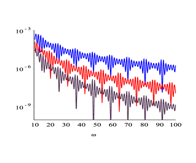
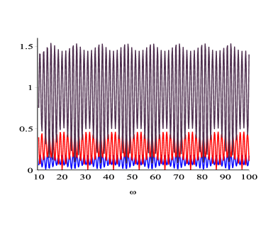
Figure 1: The error of $Q_{m}^{A}[f]$ (left) and the error scaled by $\omega^{m+\frac{3}{2}}$ (right). The blue, red, violet curves correspond to $m=1,2,3$, respectively.

A major disadvantage of the asymptotic method is that the error is essentially uncontrollable for a fixed $\omega$. To overcome this drawback, we will propose a new Filon-type method which achieves the same error estimate as the asymptotic method, whilst significantly improving the accuracy. Before proceeding, let us establish a helpful lemma.

Lemma 2.6.

Assume that $g(x)\in C^{\infty}[a,b]$ and $g{{}^{\prime}}(x)\neq 0$ for $x\in[a,b]$. Let

$$\varphi_{k}(x)=g{{}^{\prime}}(x)g(x)^{k},\quad k\geq 0,$$

and set

$$\mathcal{E}=\left\{v(x)~{}\bigg{|}~{}v(x)=\sum_{k=0}^{n-1}c_{k}\varphi_{k}(x),~{}c_{k}\in\mathbb{R}\right\}.$$

Then, $\mathcal{E}$ forms an extended Chebyshev space.

Proof.

With the assumption $g(x)\in C^{\infty}[a,b]$ we see that $\varphi_{k}(x)\in C^{\infty}[a,b]$. For any $v(x)\in\mathcal{E}$, we have, by setting $y=g(x)$, that

$$v(x)=\sum_{k=0}^{n-1}c_{k}\varphi_{k}(x)=g{{}^{\prime}}(x)\sum_{k=0}^{n-1}c_{k}y^{k}.$$

On the one hand, we can see that $v(x)\equiv 0$ implies that $c_{k}=0$, $k=0,\ldots,n-1$, and therefore $\{\varphi_{0}(x),\ldots,\varphi_{n-1}(x)\}$ forms a basis of $\mathcal{E}$. On the other hand, we can see that $v(x)$ has at most $n-1$ zeros in $[a,b]$ counting multiplicities. From [25, Theorem 2.33], it follows that $\mathcal{E}$ is an extended Chebyshev space. This completes the proof. ∎

We are now ready to construct a new Filon-type method, which is a modification of the standard method presented in [15, 16]. Let $a=x_{0}<x_{1}<\cdots<x_{d}=b$ be a set of distinct nodes with multiplicities $m_{0},m_{1},\ldots,m_{d}$ and $\sum_{k=0}^{d}m_{k}=n$. From [25, Theorem 9.9] we know that there exists a unique function $p(x)=\sum_{k=0}^{n-1}c_{k}\varphi_{k}(x)\in\mathcal{E}$ such that

$$p^{(j-1)}(x_{k})=f^{(j-1)}(x_{k}),$$ (2.9)

for all $j=1,\ldots,m_{k}$ and $k=0,\ldots,d$. The modified Filon-type method is defined by

$$Q^{F}[f]:=\mathcal{H}_{\nu}[p]=\sum_{k=0}^{n-1}c_{k}\mu_{k,\nu}^{\omega},$$ (2.10)

where we have introduced the modified moments $\mu_{k,\nu}^{\omega}=\mathcal{H}_{\nu}[\varphi_{k}]$.

Theorem 2.7.

Let $m_{0},m_{d}\geq m$, then

$$\mathcal{H}_{\nu}[f]-Q^{F}[f]=\mathcal{O}(\omega^{-m-\frac{3}{2}}),\quad\omega\rightarrow\infty.$$ (2.11)

Proof.

Let $h(x)=f(x)-p(x)$ and thus $\mathcal{H}_{\nu}[f]-Q^{F}[f]=\mathcal{H}_{\nu}[h]$. Using the expansion (2.1) we obtain

$$\mathcal{H}_{\nu}[f]-Q^{F}[f]\sim-\sum_{k=1}^{\infty}\frac{1}{(-\omega)^{k}}\left\{\frac{\sigma_{k-1}[h](b)}{g{{}^{\prime}}(b)}J_{\nu+k}(\omega g(b))-\frac{\sigma_{k-1}[h](a)}{g{{}^{\prime}}(a)}J_{\nu+k}(\omega g(a))\right\}.$$

Note that each $\sigma_{k}[h](x)$ is a linear combination of $h(x),h{{}^{\prime}}(x),\ldots,h^{(k)}(x)$. This together with the condition $m_{0},m_{d}\geq m$ implies

$$\sigma_{k}[h](a)=\sigma_{k}[h](b)=0,\quad k=0,\ldots,m-1.$$

Hence the desired result follows. ∎

We reconsider the previous example using three different modified Filon-type methods: $Q^{F}[f]$ with nodes $\{1,2\}$ and multiplicities all one, $Q^{F}[f]$ with nodes $\{1,\frac{4}{3},\frac{5}{3},2\}$ and multiplicities all one and $Q^{F}[f]$ with nodes $\{1,\frac{4}{3},\frac{5}{3},2\}$ and multiplicities all two. The modified moments $\{\mu_{k,\nu}^{\omega}\}_{k=0}^{n-1}$ are evaluated by using Theorem B.1 in the appendix. Numerical results are shown in Figure 2. As can be seen, the accuracy of the proposed method can be improved greatly by adding more derivatives interpolation at both endpoints or by adding more interior nodes. Moreover, a desired accuracy level can be achieved only with a small number of nodes and multiplicities.

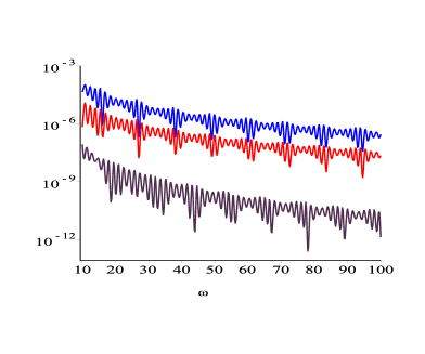
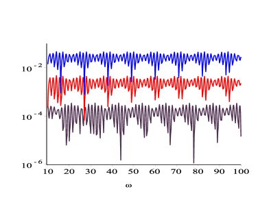
Figure 2: The left panel shows the error of $Q^{F}[f]$ with nodes $\{1,2\}$ and multiplicities all one (blue), $Q^{F}[f]$ with nodes $\{1,\frac{4}{3},\frac{5}{3},2\}$ and multiplicities all one (red) and $Q^{F}[f]$ with nodes $\{1,\frac{4}{3},\frac{5}{3},2\}$ and multiplicities all two (violet). The right panel shows the error of the first two methods scaled by $\omega^{\frac{5}{2}}$ and the error of the last method scaled by $\omega^{\frac{7}{2}}$.

2.2 The case of zeros

In this subsection we consider the case that $g(x)$ has zeros in the integration interval $[a,b]$ and we shall assume that $\Re(\nu)>-1$ to ensure the existence of the transform. Moreover, we restrict ourselves to the case where the function $g(x)$ has a single zero on the interval $[a,b]$, e.g., $g(\xi)=0$ where $\xi\in[a,b]$ and $g(x)\neq 0$ for $x\in[a,b]\backslash\{\xi\}$. If $g(x)$ has a finite number of zeros on the interval $[a,b]$, we can divide the whole interval into subintervals such that on each subinterval the function $g(x)$ contains only a single zero.

Before proceeding, let us explain why the expansion in Theorem 2.1 fails when $g(x)$ has a zero in $[a,b]$. Suppose that $\sigma_{k}[f](x)\in C^{\infty}[a,b]$ for some $k\geq 0$, it follows from (2.2) that

$$\sigma_{k+1}[f](x) =g(x)^{\nu+k+1}\frac{d}{dx}\left[\frac{\sigma_{k}[f](x)}{g(x)^{\nu+k+1}g{{}^{\prime}}(x)}\right]$$

$$=\frac{\sigma_{k}[f]{{}^{\prime}}(x)}{g{{}^{\prime}}(x)}-\frac{\sigma_{k}[f](x)g{{}^{\prime\prime}}(x)}{g{{}^{\prime}}(x)^{2}}-(\nu+k+1)\frac{\sigma_{k}[f](x)}{g(x)}$$

$$=\frac{d}{dx}\left[\frac{\sigma_{k}[f](x)}{g{{}^{\prime}}(x)}\right]-(\nu+k+1)\frac{\sigma_{k}[f](x)}{g(x)}.$$ (2.12)

We can see clearly that a simple pole at $x=\xi$ is introduced in the term $\sigma_{k}[f](x)/g(x)$ and thus integration by parts in Theorem 2.1 is no longer valid. To remedy this, we may subtract the value $\sigma_{k}[f](\xi)$ from $\sigma_{k}[f](x)$ before performing integration by parts and thus the resulting $\sigma_{k+1}[f](x)$ has a removable singularity at $x=\xi$.

Theorem 2.8.

Let $f(x),g(x)\in C^{\infty}[a,b]$ and $g{{}^{\prime}}(x)\neq 0$ for $x\in[a,b]$. Furthermore, assume that $g(\xi)=0$ for some $\xi\in[a,b]$ and $g(x)\neq 0$ for $x\in[a,b]\setminus\{\xi\}$. Then, for $\omega\rightarrow\infty$,

$$\mathcal{H}_{\nu}[f] \sim\sum_{k=0}^{\infty}\frac{\widetilde{\sigma}_{k}[f](\xi)}{(-\omega)^{k}}M(\nu+k,\omega)-\sum_{k=1}^{\infty}\frac{1}{(-\omega)^{k}}\left\{\frac{\widetilde{\sigma}_{k-1}[f](b)-\widetilde{\sigma}_{k-1}[f](\xi)}{g{{}^{\prime}}(b)}J_{\nu+k}(\omega g(b))\right.$$

$$~{}~{}~{}~{}~{}\left.-\frac{\widetilde{\sigma}_{k-1}[f](a)-\widetilde{\sigma}_{k-1}[f](\xi)}{g{{}^{\prime}}(a)}J_{\nu+k}(\omega g(a))\right\},$$ (2.13)

where $\widetilde{\sigma}_{k}[f](x)$ are defined by

$$\widetilde{\sigma}_{0}[f](x)=f(x),\quad\widetilde{\sigma}_{k}[f](x)=g(x)^{\nu+k}\frac{d}{dx}\left[\frac{\widetilde{\sigma}_{k-1}[f](x)-\widetilde{\sigma}_{k-1}[f](\xi)}{g(x)^{\nu+k}g{{}^{\prime}}(x)}\right],\quad k\geq 1.$$ (2.14)

Proof.

For each $m\geq 0$, we first rewrite $\mathcal{H}_{\nu+m}[\widetilde{\sigma}_{m}[f]]$ as

$$\mathcal{H}_{\nu+m}[\widetilde{\sigma}_{m}[f]] =\int_{a}^{b}\widetilde{\sigma}_{m}[f](x)J_{\nu+m}(\omega g(x))dx$$

$$=\widetilde{\sigma}_{m}[f](\xi)\int_{a}^{b}J_{\nu+m}(\omega g(x))dx+\int_{a}^{b}(\widetilde{\sigma}_{m}[f](x)-\widetilde{\sigma}_{m}[f](\xi))J_{\nu+m}(\omega g(x))dx$$

$$=\widetilde{\sigma}_{m}[f](\xi)M(\nu+m,\omega)+\int_{a}^{b}(\widetilde{\sigma}_{m}[f](x)-\widetilde{\sigma}_{m}[f](\xi))J_{\nu+m}(\omega g(x))dx.$$

Making use of integration by part to the last term, we find

$$\mathcal{H}_{\nu+m}[\widetilde{\sigma}_{m}[f]] =\widetilde{\sigma}_{m}[f](\xi)M(\nu+m,\omega)$$

$$~{}~{}~{}~{}~{}+\frac{1}{\omega}\int_{a}^{b}\frac{\widetilde{\sigma}_{m}[f](x)-\widetilde{\sigma}_{m}[f](\xi)}{g{{}^{\prime}}(x)g(x)^{\nu+m+1}}\frac{d}{dx}\left[g(x)^{\nu+m+1}J_{\nu+m+1}(\omega g(x))\right]dx$$

$$=\widetilde{\sigma}_{m}[f](\xi)M(\nu+m,\omega)$$

$$~{}~{}~{}~{}~{}+\frac{1}{\omega}\left\{\frac{\widetilde{\sigma}_{m}[f](b)-\widetilde{\sigma}_{m}[f](\xi)}{g{{}^{\prime}}(b)}J_{\nu+m+1}(\omega g(b))\right.$$

$$~{}~{}~{}~{}~{}\left.-\frac{\widetilde{\sigma}_{m}[f](a)-\widetilde{\sigma}_{m}[f](\xi)}{g{{}^{\prime}}(a)}J_{\nu+m+1}(\omega g(a))\right\}-\frac{1}{\omega}\mathcal{H}_{\nu+m+1}[\widetilde{\sigma}_{m+1}[f]].$$

Finally, the expansion (2.8) can be obtained by iterating the above process from $m=0$ to $m\rightarrow\infty$.

∎

The following corollary is an immediate consequence of Theorem 2.8, which has been proved in [33].

Corollary 2.9.

In the case $g(x)=x$ and $0=a<b$, then

$$\mathcal{H}_{\nu}[f] \sim\sum_{k=0}^{\infty}\frac{\widetilde{\sigma}_{k}[f](0)}{(-\omega)^{k}}M(\nu+k,\omega)-\sum_{k=1}^{\infty}\frac{\widetilde{\sigma}_{k-1}[f](b)-\widetilde{\sigma}_{k-1}[f](0)}{(-\omega)^{k}}J_{\nu+k}(\omega b).$$

where $\widetilde{\sigma}_{k}[f](x)$ are defined as in (2.14).

Proof.

Note that $\xi=0$, the desired result follows from (2.8). ∎

We now turn to investigate the dependence of $\widetilde{\sigma}_{k}[f](x)$ on $f(x)$ and its derivatives. When $x\neq\xi$, it is easy to verify that each $\widetilde{\sigma}_{k}[f](x)$ is a linear combination of $f(x),f{{}^{\prime}}(x),\ldots,f^{(k)}(x)$. When $x=\xi$, applying L’Hôspital’s rule, we obtain

$$\widetilde{\sigma}_{1}[f](\xi) =-\frac{\nu}{g{{}^{\prime}}(\xi)}f{{}^{\prime}}(\xi),$$

$$\widetilde{\sigma}_{2}[f](\xi) =-\frac{\nu+1}{(g{{}^{\prime}}(\xi))^{3}}\left[\frac{\nu-3}{2}g{{}^{\prime\prime}}(\xi)f{{}^{\prime}}(\xi)-\frac{\nu-1}{2}g{{}^{\prime}}(\xi)f{{}^{\prime\prime}}(\xi)\right],$$ (2.15)

$$\widetilde{\sigma}_{3}[f](\xi) =-\frac{\nu+2}{(g{{}^{\prime}}(\xi))^{5}}\left[\left(\frac{8\nu-\nu^{2}}{6}g{{}^{\prime}}(\xi)g{{}^{\prime\prime\prime}}(\xi)+\frac{\nu^{2}-8\nu+3}{2}(g{{}^{\prime\prime}}(\xi))^{2}\right)f{{}^{\prime}}(\xi)\right.$$

$$~{}~{}~{}~{}~{}~{}~{}~{}~{}-\frac{\nu^{2}-4\nu+1}{2}g{{}^{\prime}}(\xi)g{{}^{\prime\prime\prime}}(\xi)f{{}^{\prime\prime}}(\xi)\left.+\frac{\nu^{2}-2\nu}{6}(g{{}^{\prime}}(\xi))^{2}f{{}^{\prime\prime\prime}}(\xi)\right],$$

and it is not difficult to verify that each $\widetilde{\sigma}_{k}[f](\xi)$ is a linear combination of $f{{}^{\prime}}(\xi),f{{}^{\prime\prime}}(\xi),\ldots,$ $f^{(k)}(\xi)$. In the particular case where $g(x)=x$, $\xi=0$ and assume that $f(x)$ is analytic inside a neighborhood of the origin, the values $\widetilde{\sigma}_{k}[f](0)$ are a scalar multiple of $f^{(k)}(0)$ (see [26, Theorem C.3] or [27])

$$\widetilde{\sigma}_{k}[f](0)=\frac{f^{(k)}(0)}{k!}\prod_{\ell=0}^{k-1}\left(1+2\ell-\nu-k\right),\quad k\geq 1.$$ (2.16)

Truncating (2.8) after the first $m$ terms, yields an asymptotic method

$$Q_{m}^{A}[f] =\sum_{k=0}^{m-1}\frac{\widetilde{\sigma}_{k}[f](\xi)}{(-\omega)^{k}}M(\nu+k,\omega)-\sum_{k=1}^{m}\frac{1}{(-\omega)^{k}}\left\{\frac{\widetilde{\sigma}_{k-1}[f](b)-\widetilde{\sigma}_{k-1}[f](\xi)}{g{{}^{\prime}}(b)}J_{\nu+k}(\omega g(b))\right.$$

$$~{}~{}~{}~{}~{}~{}~{}~{}~{}~{}~{}~{}~{}~{}~{}\left.-\frac{\widetilde{\sigma}_{k-1}[f](a)-\widetilde{\sigma}_{k-1}[f](\xi)}{g{{}^{\prime}}(a)}J_{\nu+k}(\omega g(a))\right\}.$$ (2.17)

Moreover, from the above discussion that the method (2.2) is a linear combination of the values $f(a),f{{}^{\prime}}(a),\ldots,f^{(m-1)}(a)$, $f(\xi),f{{}^{\prime}}(\xi),\ldots,$ $f^{(m-1)}(\xi)$ and $f(b),f{{}^{\prime}}(b),\ldots,f^{(m-1)}(b)$.

Now, we are in a position to prove the error estimate for the asymptotic method (2.2). Before stating the result, it will be helpful to show the estimate of $M(\nu,\omega)$.

Lemma 2.10.

Let $g(x)\in C^{\infty}[a,b]$ and $g{{}^{\prime}}(x)\neq 0$ for $x\in[a,b]$. Furthermore, assume that $g(\xi)=0$ for some $\xi\in[a,b]$ and $g(x)\neq 0$ for $x\in[a,b]\setminus\{\xi\}$. Then, for $\omega\rightarrow\infty$,

$$M(\nu,\omega)=\mathcal{O}(\omega^{-1}).$$ (2.18)

Proof.

Since $g{{}^{\prime}}(x)\neq 0$ for $x\in[a,b]$ this implies that $g(x)$ is a strictly monotonic function on the interval $[a,b]$. Without loss of generality, we may assume that $g(x)$ is a monotonically increasing function, i.e., $g(a)\leq 0\leq g(b)$.

Split the integral representation of $M(\nu,\omega)$ into integrals over $[a,\xi]$ and $[\xi,b]$, we have

$$M(\nu,\omega) =\int_{a}^{\xi}J_{\nu}(\omega g(x))dx+\int_{\xi}^{b}J_{\nu}(\omega g(x))dx.$$

$$=\int_{0}^{-g(a)}\frac{1}{g{{}^{\prime}}(g^{-1}(-t))}J_{\nu}(-\omega t)dt+\int_{0}^{g(b)}\frac{1}{g{{}^{\prime}}(g^{-1}(t))}J_{\nu}(\omega t)dt,$$

where we have made the change of variable $t=-g(x)$ in the first integral and $t=g(x)$ in the second. By making use of the identity $J_{\nu}(-z)=e^{\nu\pi i}J_{\nu}(z)$ [20, Eqn. 10.11.1], we can rewrite $M(\nu,\omega)$ as

$$M(\nu,\omega) =e^{\nu\pi i}\int_{0}^{-g(a)}\frac{1}{g{{}^{\prime}}(g^{-1}(-t))}J_{\nu}(\omega t)dt+\int_{0}^{g(b)}\frac{1}{g{{}^{\prime}}(g^{-1}(t))}J_{\nu}(\omega t)dt.$$ (2.19)

Using Corollary 2.9 and keeping only the leading terms, we have

$$M(\nu,\omega) \sim\frac{1}{g{{}^{\prime}}(\xi)}\left[e^{\nu\pi i}\int_{0}^{-g(a)}J_{\nu}(\omega t)dt+\int_{0}^{g(b)}J_{\nu}(\omega t)dt\right]$$

$$~{}~{}~{}~{}~{}+\frac{e^{\nu\pi i}}{\omega}\left[\frac{1}{g{{}^{\prime}}(a)}-\frac{1}{g{{}^{\prime}}(\xi)}\right]J_{\nu+1}(-\omega g(a))+\frac{1}{\omega}\left[\frac{1}{g{{}^{\prime}}(b)}-\frac{1}{g{{}^{\prime}}(\xi)}\right]J_{\nu+1}(\omega g(b)).$$

To estimate $M(\nu,\omega)$, it suffices to derive estimates of those terms on the right-hand side. For the first term, from Lemma A.1 in the appendix we see that both integrals inside the bracket behave like $\mathcal{O}(\omega^{-1})$ for fixed $\nu$ and $\Re(\nu)>-1$. For the second and third terms, it is easy to see that both terms behave like $\mathcal{O}(\omega^{-\frac{3}{2}})$. Hence, the desired result follows. ∎

Owing to Lemma 2.10, we have the following estimate.

Theorem 2.11.

Under the same assumptions as in Theorem 2.8, it follows that, for $\omega\rightarrow\infty$,

$$\mathcal{H}_{\nu}[f]-Q_{m}^{A}[f]=\left\{\begin{array}[]{cc}{\displaystyle\mathcal{O}(\omega^{-m-1})},&\mbox{if $\widetilde{\sigma}_{m}[f](\xi)\neq 0$},\\[10.0pt] {\displaystyle\mathcal{O}(\omega^{-m-\frac{3}{2}})},&\mbox{if $\widetilde{\sigma}_{m}[f](\xi)=0$},\end{array}\right.$$ (2.22)

where $Q_{m}^{A}[f]$ is defined as in (2.2).

Proof.

Combining (2.8) and (2.2), we see that

$$\mathcal{H}_{\nu}[f]-Q_{m}^{A}[f] \sim\sum_{k=m}^{\infty}\frac{\widetilde{\sigma}_{k}[f](\xi)}{(-\omega)^{k}}M(\nu+k,\omega)$$

$$~{}~{}~{}~{}~{}-\sum_{k=m+1}^{\infty}\frac{1}{(-\omega)^{k}}\left\{\frac{\widetilde{\sigma}_{k-1}[f](b)-\widetilde{\sigma}_{k-1}[f](\xi)}{g{{}^{\prime}}(b)}J_{\nu+k}(\omega g(b))\right.$$ (2.23)

$$~{}~{}~{}~{}~{}\left.-\frac{\widetilde{\sigma}_{k-1}[f](a)-\widetilde{\sigma}_{k-1}[f](\xi)}{g{{}^{\prime}}(a)}J_{\nu+k}(\omega g(a))\right\}.$$

It is clear that the behavior of the left-hand side is determined by comparing the behavior of those two sums on the right-hand side. Thanks to Lemma 2.10, we can deduce that the first sum on the right-hand side of (2.2) behaves like $\mathcal{O}(\omega^{-m-1})$ if $\widetilde{\sigma}_{m}[f](\xi)\neq 0$ and $\mathcal{O}(\omega^{-m-2})$ if $\widetilde{\sigma}_{m}[f](\xi)=0$. For the second sum, we easily see that it behaves like $\mathcal{O}(\omega^{-m-\frac{3}{2}})$. Combining these estimates gives the desired result. ∎

As a simple example, we consider $f(x)=\sin x$, $g(x)=x$, $\nu=2$ and $[a,b]=[0,1]$. Clearly, $g(x)$ has a unique zero at $\xi=0$. Moreover, from (2.16) we can check easily that $\sigma_{1}[f](\xi)=-2$ and $\sigma_{k}[f](\xi)=0$ for $k=2,3$. Thus, we can expect that the decay rate of the error of $Q_{m}^{A}[f]$ is $\mathcal{O}(\omega^{-m-1})$ for $m=1$ and is $\mathcal{O}(\omega^{-m-\frac{3}{2}})$ for $m=2,3$. In our computations, the moments $M(\nu+k,\omega)$ are evaluated by (A.2) in the appendix directly. Numerical results are illustrated in Figure 3 and we can see that they are in good agreement with our analysis.

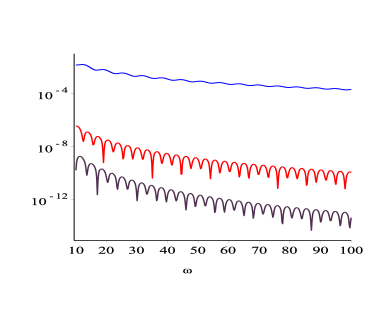
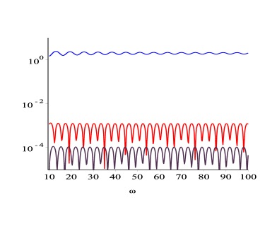
Figure 3: The error of $Q_{m}^{A}[f]$ (left) and the error of $Q_{1}^{A}[f]$ scaled by $\omega^{2}$ and the error of $Q_{m}^{A}[f]$ scaled by $\omega^{m+\frac{3}{2}}$ for $m=2,3$ (right). The blue, red and violet curves correspond to $m=1,2,3$, respectively.

Remark 2.12.

When using the asymptotic method (2.2), it is necessary to evaluate the moments $M(\nu+k,\omega)$. As will be shown below, modified Filon-type methods in Theorem 2.13 can be used to evaluate them accurately; see Figure 4 for an illustration.

We now consider to construct a modified Filon-type method. Note that the zero of $g(x)$ is a critical point of the transform, so we need to impose interpolation conditions at this point. Let $x_{\ell}=\xi$ for some $\ell\in\{0,\ldots,d\}$ and let $p(x)=\sum_{k=0}^{n-1}c_{k}\varphi_{k}(x)\in\mathcal{E}$ be the unique function that satisfies the interpolation conditions (2.9) and let $Q^{F}[f]=\mathcal{H}_{\nu}[p]$.

Theorem 2.13.

Let $m_{0},m_{\ell},m_{d}\geq m$, then

$$\mathcal{H}_{\nu}[f]-Q^{F}[f]=\left\{\begin{array}[]{cc}{\displaystyle\mathcal{O}(\omega^{-m-1})},&\mbox{if $\widetilde{\sigma}_{m}[f-p](\xi)\neq 0$},\\[10.0pt] {\displaystyle\mathcal{O}(\omega^{-m-\frac{3}{2}})},&\mbox{if $\widetilde{\sigma}_{m}[f-p](\xi)=0$}.\end{array}\right.$$ (2.26)

Proof.

Let $h(x)=f(x)-p(x)$ and we clearly have $\mathcal{H}_{\nu}[f]-Q^{F}[f]=\mathcal{H}_{\nu}[h]$. Additionally, from the interpolation conditions and the dependence of $\widetilde{\sigma}_{k}[f](x)$ on $f(x)$ and its derivatives, we obtain

$$\widetilde{\sigma}_{k}[h](a)=\widetilde{\sigma}_{k}[h](\xi)=\widetilde{\sigma}_{k}[h](b)=0,\quad k=0,\ldots,m-1.$$

The result follows from Theorem 2.11. ∎

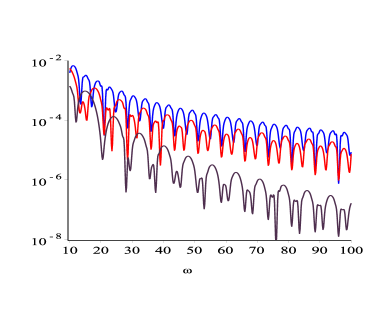
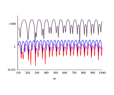
Figure 4: The left panel shows the error of $Q^{F}[f]$ with nodes $\{0,1\}$ and multiplicities all one (blue), $Q^{F}[f]$ with the nodes $\{0,\frac{1}{3},\frac{2}{3},1\}$ and multiplicities all one (red) and $Q^{F}[f]$ with nodes $\{0,\frac{1}{3},\frac{2}{3},1\}$ and multiplicities $\{3,1,1,3\}$ (violet). The right panel shows the error of the first two methods scaled by $\omega^{\frac{5}{2}}$ and the last one scaled by $\omega^{\frac{9}{2}}$.

As an example, we consider the evaluation of the following moment

$$M(0,\omega)=\int_{0}^{1}J_{0}(\omega\sin x)dx.$$ (2.27)

This moment is a finite Hankel transform with $f(x)=1$, $g(x)=\sin x$, $\nu=0$ and $\xi=0$. We compare the accuracy of three modified Filon-type methods: $Q^{F}[f]$ with nodes $\{0,1\}$ and multiplicities all one, $Q^{F}[f]$ with the nodes $\{0,\frac{1}{3},\frac{2}{3},1\}$ and multiplicities all one and $Q^{F}[f]$ with the nodes $\{0,\frac{1}{3},\frac{2}{3},1\}$ and multiplicities $\{3,1,1,3\}$. For the first two methods, they correspond to $m=1$ and it is easy to check from (2.2) that $\widetilde{\sigma}_{1}[f-p](0)=0$. Thus, the decay rate of the error of both methods is $\mathcal{O}(\omega^{-\frac{5}{2}})$. For the last method, we can see that $m=3$ and we can check from (2.2) that $\widetilde{\sigma}_{3}[f-p](0)=-(f{{}^{\prime\prime}}(0)-p{{}^{\prime\prime}}(0))=0$. Therefore, the decay rate of its error is $\mathcal{O}(\omega^{-\frac{9}{2}})$. In our implementation, the modified moments $\{\mu_{k,\nu}^{\omega}\}_{k=0}^{n-1}$ are evaluated by Theorem B.1 in the appendix. Numerical results are presented in Figure 4. Clearly, we can see that the decay rates of these three methods are consistent with the expected rates.

3 The case of stationary points

When $g{{}^{\prime}}(\zeta)=0$ for some $\zeta\in[a,b]$, we call $x=\zeta$ a stationary point. Further, we call $x=\zeta$ a stationary point of order $r$ if $g^{(j)}(\zeta)=0$, $j=1,\ldots,r$, where $r\geq 1$ and $g^{(r+1)}(\zeta)\neq 0$.

In this section, we restrict our attention to the case that $g(x)$ has only one stationary point of order $r$ at $x=\zeta\in[a,b]$, i.e., $g{{}^{\prime}}(x)\neq 0$ for $x\in[a,b]\backslash\{\zeta\}$. We also assume that $g(x)\neq 0$ for $x\in[a,b]\backslash\{\zeta\}$. The stationary point can be classified into the following two types:

1. Type I: $g(\zeta)\neq 0$.

2. Type II: $g(\zeta)=0$.

Here we shall restrict our analysis to the latter case, i.e., $x=\zeta$ is a stationary point of type II, since a similar analysis can be performed for the former case. Moreover, we point out that if $g(x)$ has a zero at $x=\overline{\zeta}\in[a,b]$ and $\overline{\zeta}\neq\zeta$, then we can divide the interval $[a,b]$ into two subintervals such that one contains the zero $x=\overline{\zeta}$ and the other contains the stationary point $x=\zeta$. To ensure the existence of the transform, we shall assume throughout this section that $\Re(\nu)>-\frac{1}{r+1}$.

3.1 Asymptotic expansions

In order to gain insight into the mechanism of performing integration by parts when $g(x)$ has a stationary point, we return to Theorem 2.1 again. From (2.2) we can see that a pole at $x=\zeta$ is introduced in the term inside the bracket $\sigma_{k}[f](x)/g{{}^{\prime}}(x)$ and the term $\sigma_{k}[f](x)/g(x)$. The existence of pole implies that (2.2) is still no longer valid. However, this problem can be circumvented by subtracting the first several terms of $\sigma_{k}[f](x)$ about $x=\zeta$ before we perform integration by parts. Note that both $\sigma_{k}[f](x)/g{{}^{\prime}}(x)$ and $\sigma_{k}[f](x)/g(x)$ have a pole at $x=\zeta$ and the pole is of order $r$ for the former and is of order $r+1$ for the latter. It is sufficient to subtract the first $r+1$ terms of the Taylor expansion of $\sigma_{k}[f](x)$ about $x=\zeta$ to ensure that the resulting $\sigma_{k+1}[f](x)$ has a removable singularity.

For simplicity in exposition, let us define

$$T_{r}[f](x,y)=\sum_{j=0}^{r}\frac{f^{(j)}(y)}{j!}(x-y)^{j}.$$ (3.1)

We start from the case that $x=\zeta$ is an interior stationary point, i.e., $\zeta\in(a,b)$.

Theorem 3.1.

Assume that $f(x),g(x)\in C^{\infty}[a,b]$ and $g(x)$ has a stationary point of type II and of order $r$ at $x=\zeta\in(a,b)$. Furthermore, we assume that $g(x),g{{}^{\prime}}(x)\neq 0$ for $x\in[a,b]\setminus\{\zeta\}$. Then, for $\omega\rightarrow\infty$,

$$\mathcal{H}_{\nu}[f] \sim\sum_{k=0}^{\infty}\frac{1}{(-\omega)^{k}}\sum_{j=0}^{r}\frac{\widehat{\sigma}_{k}[f]^{(j)}(\zeta)}{j!}M_{j}(\zeta,\nu+k,\omega)$$

$$~{}~{}~{}~{}~{}-\sum_{k=1}^{\infty}\frac{1}{(-\omega)^{k}}\left\{\frac{\widehat{\sigma}_{k-1}[f](b)-T_{r}[\widehat{\sigma}_{k-1}](b,\zeta)}{g{{}^{\prime}}(b)}J_{\nu+k}(\omega g(b))\right.$$ (3.2)

$$~{}~{}~{}~{}~{}\left.-\frac{\widehat{\sigma}_{k-1}[f](a)-T_{r}[\widehat{\sigma}_{k-1}](a,\zeta)}{g{{}^{\prime}}(a)}J_{\nu+k}(\omega g(a))\right\},$$

where

$$\widehat{\sigma}_{0}[f](x)=f(x),~{}~{}\widehat{\sigma}_{k}[f](x)=g(x)^{\nu+k}\frac{d}{dx}\left[\frac{\displaystyle\widehat{\sigma}_{k-1}[f](x)-T_{r}[\widehat{\sigma}_{k-1}](x,\zeta)}{g(x)^{\nu+k}g{{}^{\prime}}(x)}\right],~{}k\geq 1.$$ (3.3)

Proof.

The proof is similar to that of Theorem 2.8. We omit the details. ∎

When the stationary point $x=\zeta$ is at an endpoint, the result in Theorem 3.1 should be modified slightly. Without loss of generality, we assume that the stationary point is located at the left endpoint, i.e., $\zeta=a$.

Theorem 3.2.

Assume that $f(x),g(x)\in C^{\infty}[a,b]$ and $g(x)$ has a stationary point of type II and of order $r$ at $x=a$. Furthermore, we assume that $g(x),g{{}^{\prime}}(x)\neq 0$ for $x\in(a,b]$. Then, for $\omega\rightarrow\infty$,

$$\mathcal{H}_{\nu}[f] \sim\sum_{k=0}^{\infty}\frac{1}{(-\omega)^{k}}\sum_{j=0}^{r}\frac{\widehat{\sigma}_{k}[f]^{(j)}(a)}{j!}M_{j}(a,\nu+k,\omega)$$

$$~{}~{}~{}~{}~{}-\sum_{k=1}^{\infty}\frac{1}{(-\omega)^{k}}\left[\frac{\widehat{\sigma}_{k-1}[f](b)-T_{r}[\widehat{\sigma}_{k-1}](b,a)}{g{{}^{\prime}}(b)}\right]J_{\nu+k}(\omega g(b)),$$ (3.4)

where $\widehat{\sigma}_{k}[f](x)$ are defined as in (3.3).

Proof.

Note that

$$\lim_{x\rightarrow a}\frac{\widehat{\sigma}_{k-1}[f](x)-T_{r}[\widehat{\sigma}_{k-1}](x,a)}{g{{}^{\prime}}(x)}=0.$$

The expansion (3.2) follow from Theorem 3.1. ∎

As a consequence of Theorem 3.2, we have the following result.

Corollary 3.3.

In the simplest case $g(x)=x^{r+1}$ and $0=a<b$, then

$$\mathcal{H}_{\nu}[f] \sim\sum_{k=0}^{\infty}\frac{1}{(-\omega)^{k}}\sum_{j=0}^{r}\frac{\widehat{\sigma}_{k}[f]^{(j)}(0)}{j!}M_{j}(0,\nu+k,\omega)$$

$$~{}~{}~{}~{}~{}-\sum_{k=1}^{\infty}\frac{1}{(-\omega)^{k}}\bigg{[}\widehat{\sigma}_{k-1}[f](b)-T_{r}[\widehat{\sigma}_{k-1}](b,0)\bigg{]}\frac{J_{\nu+k}(\omega b^{r+1})}{(r+1)b^{r}}.$$ (3.5)

where $\widehat{\sigma}_{k}[f](x)$ are defined as in (3.3).

Proof.

It follows immediately from Theorem 3.2. ∎

We now clarify the dependence of $\widehat{\sigma}_{k}[f](x)$ on $f(x)$ and its derivatives. When $x\neq\zeta$, one can easily verify that each $\widehat{\sigma}_{k}[f](x)$ is a linear combination of $f(x),f{{}^{\prime}}(x),\ldots,f^{(k)}(x)$. In the case $x=\zeta$ and assume that $f$ and $g$ are analytic functions in a neighborhood of the interval $[a,b]$, from Theorem C.2 in the appendix we know that each $\widehat{\sigma}_{k}[f]^{(j)}(\zeta)$ is a linear combination of the values $f^{(r+1+j)}(\zeta),f^{(r+2+j)}(\zeta),$ $\ldots,f^{(k(r+1)+j)}(\zeta)$.

As before, the asymptotic methods can be defined by truncating the expansion in Theorem 3.1 when $\zeta\in(a,b)$ and by truncating the expansion in Theorem 3.2 when $\zeta=a$. For simplicity of presentation, we only consider the latter case. The asymptotic method is defined by

$$Q_{m}^{A}[f] =\sum_{k=0}^{m-1}\frac{1}{(-\omega)^{k}}\sum_{j=0}^{r}\frac{\widehat{\sigma}_{k}[f]^{(j)}(a)}{j!}M_{j}(a,\nu+k,\omega)$$

$$~{}~{}~{}~{}~{}-\sum_{k=1}^{m}\frac{1}{(-\omega)^{k}}\bigg{[}\frac{\widehat{\sigma}_{k-1}[f](b)-T_{r}[\widehat{\sigma}_{k-1}](b,a)}{g{{}^{\prime}}(b)}\bigg{]}J_{\nu+k}(\omega g(b)).$$ (3.6)

Moreover, the above discussion shows that the method $Q_{m}^{A}[f]$ is a linear combination of the values $f(b),f{{}^{\prime}}(b),\ldots,f^{(m-1)}(b)$ and $f(a),f{{}^{\prime}}(a),\ldots,f^{(m(r+1)-1)}(a)$.

3.2 Error estimate

To derive error estimates of the asymptotic method $Q_{m}^{A}[f]$ defined in (3.1), we need to show the estimate of $M_{j}(\zeta,\nu,\omega)$.

Lemma 3.4.

Assume that $g(x)\in C^{\infty}[a,b]$ and $g(x)$ has a stationary point of type II and of order $r$ at $x=\zeta\in[a,b]$. Furthermore, assume that $g(x),g{{}^{\prime}}(x)\neq 0$ for $x\in[a,b]\setminus\{\zeta\}$. Then, for $0\leq j\leq r$ and $\omega\rightarrow\infty$,

$$M_{j}(\zeta,\nu,\omega)=\mathcal{O}(\omega^{-\frac{j+1}{r+1}}).$$ (3.7)

Proof.

From the assumption $g{{}^{\prime}}(x)\neq 0$ for $x\in[a,b]\setminus\{\zeta\}$, we see that $g(x)$ is strictly monotonically on each subinterval $[a,\zeta]$ and $[\zeta,b]$. For simplicity, we only consider the case where $g(x)$ is strictly decreasing on $[a,\zeta]$ and is strictly increasing on $[\zeta,b]$, i.e., $g(a)\geq 0$ and $g(b)\geq 0$. Splitting the integral representation of $M_{j}(\zeta,\nu,\omega)$ at $x=\zeta$ gives

$$M_{j}(\zeta,\nu,\omega) =\int_{a}^{\zeta}(x-\zeta)^{j}J_{\nu}(\omega g(x))dx+\int_{\zeta}^{b}(x-\zeta)^{j}J_{\nu}(\omega g(x))dx$$

$$=\int_{\sqrt[r+1]{g(a)}}^{0}y^{j}h(y)J_{\nu}(\omega y^{r+1})dy+\int_{0}^{\sqrt[r+1]{g(b)}}y^{j}h(y)J_{\nu}(\omega y^{r+1})dy,$$ (3.8)

where in the last step we have made a change of variable $y^{r+1}=g(x)$ and

$$h(y)=(r+1)\frac{(x-\zeta)^{j}}{g{{}^{\prime}}(x)}y^{r-j}.$$

Note that the assumption on $g(x)$ implies that $h(y)$ is a $C^{\infty}$ function and $h(0)\neq 0$. We now consider the asymptotic behavior of the second integral on the right-hand side of (3.2). Let us define $\widehat{h}(y)=y^{j}h(y)$ and $\widehat{b}=\sqrt[r+1]{g(b)}$. By invoking Corollary 3.3 and keeping only the first term of the expansion, we have

$$\int_{0}^{\sqrt[r+1]{g(b)}}y^{j}h(y)J_{\nu}(\omega y^{r+1})dy =\int_{0}^{\widehat{b}}\widehat{h}(y)J_{\nu}(\omega y^{r+1})dy$$

$$\sim\sum_{\ell=0}^{r}\frac{\widehat{h}^{(\ell)}(0)}{\ell!}\int_{0}^{\widehat{b}}y^{\ell}J_{\nu}(\omega y^{r+1})dy$$

$$~{}~{}~{}~{}~{}+\frac{1}{\omega}\bigg{[}\widehat{h}(\widehat{b})-T_{r}[\widehat{h}](\widehat{b},0)\bigg{]}\frac{J_{\nu+1}(\omega\widehat{b}^{r+1})}{(r+1)\widehat{b}^{r}}$$

$$=\sum_{\ell=j}^{r}\frac{\widehat{h}^{(\ell)}(0)}{\ell!}\int_{0}^{\widehat{b}}y^{\ell}J_{\nu}(\omega y^{r+1})dy$$

$$~{}~{}~{}~{}~{}+\frac{1}{\omega}\bigg{[}\widehat{h}(\widehat{b})-T_{r}[\widehat{h}](\widehat{b},0)\bigg{]}\frac{J_{\nu+1}(\omega\widehat{b}^{r+1})}{(r+1)\widehat{b}^{r}},$$ (3.9)

where we have used the fact $\widehat{h}^{(\ell)}(0)=0$ for $0\leq\ell\leq j-1$ in the last step. For the integrals on the right-hand side of (3.2), by setting $t=y^{r+1}$, we have

$$\int_{0}^{\widehat{b}}y^{\ell}J_{\nu}(\omega y^{r+1})dy=\frac{1}{r+1}\int_{0}^{\widehat{b}^{r+1}}t^{\frac{\ell+1}{r+1}-1}J_{\nu}(\omega t)dt.$$

From Lemma A.1 in the appendix we know that the integral on the right-hand side behaves like $\mathcal{O}(\omega^{-\frac{\ell+1}{r+1}})$ for fixed $\nu$ and $\Re(\nu)>-\frac{1}{r+1}$. Thus, we can deduce that the first term on the right-hand side of (3.2) behaves like $\mathcal{O}(\omega^{-\frac{j+1}{r+1}})$. Moreover, it is easy to see that the second term on the right-hand side of (3.2) behaves like $\mathcal{O}(\omega^{-\frac{3}{2}})$. We can conclude that the second integral on the right-hand side of (3.2) behaves like $\mathcal{O}(\omega^{-\frac{j+1}{r+1}})$.

Finally, using a similar argument, we can show that the first integral on the right-hand side of (3.2) also behaves like $\mathcal{O}(\omega^{-\frac{j+1}{r+1}})$. This completes the proof. ∎

Theorem 3.5.

Under the same assumptions as in Theorem 3.2, we have

$$\mathcal{H}_{\nu}[f]-Q_{m}^{A}[f]=\mathcal{O}(\omega^{-m-\frac{1}{r+1}}),\quad\omega\rightarrow\infty,$$ (3.10)

where $Q_{m}^{A}[f]$ is defined as in (3.1).

Proof.

It follows by combining Theorem 3.2 and Theorem 3.4. ∎

Consider an example with $f(x)=e^{x}$, $g(x)=x^{2}$, $\nu=2$ and $[a,b]=[0,1]$. This example has a stationary point of order $r=1$ at $\zeta=0$. In our computations, we rewrite $M_{j}(\zeta,\nu+k,\omega)$ as

$$M_{j}(\zeta,\nu+k,\omega) =\int_{0}^{1}x^{j}J_{\nu+k}(\omega x^{2})dx=\frac{1}{2}\int_{0}^{1}y^{\frac{j-1}{2}}J_{\nu+k}(\omega y)dy,$$

and then the last integral is calculated by (A.2) in the appendix. In Figure 5 we display the error of $Q_{m}^{A}[f]$ in the left panel and the error scaled by $\omega^{m+\frac{1}{2}}$ in the right panel. As expected, the accuracy of $Q_{m}^{A}[f]$ improves as $\omega$ increases and the decay rate of the error of $Q_{m}^{A}[f]$ is $\mathcal{O}(\omega^{-m-\frac{1}{2}})$.

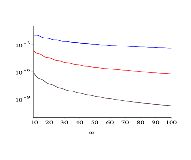
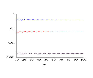
Figure 5: Absolute error of $Q_{m}^{A}[f]$ (left) and the error scaled by $\omega^{m+\frac{1}{2}}$ (right). The blue, red, violet curves correspond to $m=1,2,3$, respectively.

Now, we consider to construct a Filon-type method for the transform in the presence of a stationary point at the left endpoint. To achieve this, we introduce an auxiliary result.

Lemma 3.6.

Assume that $g(x)\in C^{\infty}[a,b]$ and it has a stationary point of type II and of order $r$ at $x=a$ and $g^{(r+1)}(x)\neq 0$ for $x\in[a,b]$. Let

$$\widehat{\varphi}_{k}(x)=\left\{\begin{array}[]{cc}{\displaystyle g{{}^{\prime}}(x)g(x)^{\frac{k-r}{r+1}}},&\mbox{if $g^{(r+1)}(x)>0$},\\[12.0pt] {\displaystyle g{{}^{\prime}}(x)(-g(x))^{\frac{k-r}{r+1}}},&\mbox{if $g^{(r+1)}(x)<0$}.\end{array}\right.$$ (3.13)

and set

$$\widehat{\mathcal{E}}=\left\{v(x)~{}\bigg{|}~{}v(x)=\sum_{k=0}^{n-1}c_{k}\widehat{\varphi}_{k}(x),~{}~{}c_{k}\in\mathbb{R}\right\}.$$

Then, $\widehat{\mathcal{E}}$ forms an extended Chebyshev space.

Proof.

Here we only consider the case of $g^{(r+1)}(x)>0$ for $x\in[a,b]$ and the other case $g^{(r+1)}(x)<0$ can be handled in a similar manner. With this condition, we can deduce that $g^{(j)}(x)>0$ for $x\in(a,b]$ and $j=1,\ldots,r$ and thus $g(x)$ is strictly increasing in $[a,b]$. Setting $y^{r+1}=g(x)$, we have

$$v(x)=\sum_{k=0}^{n-1}c_{k}\widehat{\varphi}_{k}(x)=\Lambda(x)\sum_{k=0}^{n-1}c_{k}y^{k},$$

where $\Lambda(x)=g{{}^{\prime}}(x)g(x)^{-\frac{r}{r+1}}$. Note that $\Lambda(x)$ have a removable singularity at $x=a$ and we can easily check that $\Lambda(a)=\lim_{x\rightarrow a}\Lambda(x)=(r+1)\left[g^{(r+1)}(a)/(r+1)!\right]^{\frac{1}{r+1}}>0$. Thus, we can conclude that $\Lambda(x)\in C^{\infty}[a,b]$ and $\Lambda(x)>0$ for $x\in[a,b]$. The remaining details of the proof is similar to that of Lemma 2.6 and hence are omitted. ∎

Let $a=x_{0}<x_{1}<\cdots<x_{d}=b$ be a set of distinct nodes with multiplicities $m_{0},m_{1},\ldots,m_{d}$ and $\sum_{k=0}^{d}m_{k}=n$. Suppose that $\widehat{p}(x)=\sum_{k=0}^{n-1}c_{k}\widehat{\varphi}_{k}(x)\in\widehat{\mathcal{E}}$ is the unique function which satisfies $\widehat{p}^{(j-1)}(x_{k})=f^{(j-1)}(x_{k})$ for $j=1,\ldots,m_{k}$ and $k=0,\ldots,d$. The modified Filon-type method is then defined by

$$Q^{F}[f]:=\mathcal{H}_{\nu}[\widehat{p}]=\sum_{k=0}^{n-1}c_{k}\widehat{\mu}_{k,\nu}^{\omega}.$$ (3.14)

where $\widehat{\mu}_{k,\nu}^{\omega}=\mathcal{H}_{\nu}[\widehat{\varphi}_{k}]$.

Theorem 3.7.

Under the same assumptions as in Theorem 3.2, and assume that $g^{(r+1)}(x)\neq 0$ for $x\in[a,b]$. Let $m_{d}\geq m$ and $m_{0}\geq m(r+1)$, then

$$\mathcal{H}_{\nu}[f]-Q^{F}[f]=\mathcal{O}(\omega^{-m-\frac{1}{r+1}}).$$ (3.15)

Proof.

Let $h(x)=f(x)-\widehat{p}(x)$ and we have $\mathcal{H}_{\nu}[f]-Q^{F}[f]=\mathcal{H}_{\nu}[h]$. By using the assumptions $m_{d}\geq m$ and $m_{0}\geq m(r+1)$ and the dependence relation of $\sigma_{k}[f](x)$ on $f(x)$ and its derivatives, we have for $k=0,\ldots,m-1$ that

$$\sigma_{k}[h](b)=\sigma_{k}[h]^{(j)}(a)=0,$$

where $j=0,\ldots,r$. The desired results follow from Theorem 3.5. ∎

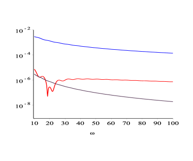
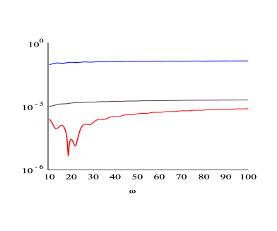
Figure 6: The left panel shows the error of $Q^{F}[f]$ with nodes $\{0,1\}$ and multiplicities $\{2,1\}$ (blue), $Q^{F}[f]$ with nodes $\{0,\frac{1}{3},\frac{2}{3},1\}$ and multiplicities $\{2,1,1,1\}$ (red) and $Q^{F}[f]$ with nodes $\{0,1\}$ and multiplicities $\{4,2\}$ (violet). The right panel shows the error of the first two methods scaled by $\omega^{\frac{3}{2}}$ and the error of the last method scaled by $\omega^{\frac{5}{2}}$.

We reconsider the example used in Figure 5. We compare the accuracy of three modified Filon-type methods: $Q^{F}[f]$ with nodes $\{0,1\}$ and multiplicities $\{2,1\}$, $Q^{F}[f]$ with nodes $\{0,\frac{1}{3},\frac{2}{3},1\}$ and multiplicities $\{2,1,1,1\}$ and $Q^{F}[f]$ with nodes $\{0,1\}$ and multiplicities $\{4,2\}$. It is easy to see that the first two Filon-type methods correspond to $m=1$ and therefore the decay rate of their error is $\mathcal{O}(\omega^{-\frac{3}{2}})$. For the last one, it corresponds to $m=2$ and therefore the decay rate of its error is $\mathcal{O}(\omega^{-\frac{5}{2}})$. In our computations, the moments $\{\widehat{\mu}_{k,\nu}^{\omega}\}_{k=0}^{n-1}$ are evaluated by using Theorem B.2 in the appendix. Numerical results are presented in Figure 6.

4 Extension

In this section we present several extensions of our results which might be interesting in applications.

4.1 Fourier-Bessel series

The Fourier-Bessel series of a function $f:[0,b]\rightarrow\mathbb{R}$ is defined by

$$f(x)\sim\sum_{k=1}^{\infty}a_{k}J_{\nu}\left(\frac{j_{\nu,k}}{b}x\right),$$ (4.1)

where $j_{\nu,k}$ is the $k$th positive root of $J_{\nu}(x)$ and the coefficients are defined by

$$a_{k}=\frac{2}{[bJ_{\nu+1}(j_{\nu,k})]^{2}}\int_{0}^{b}xf(x)J_{\nu}\left(\frac{j_{\nu,k}}{b}x\right)dx.$$ (4.2)

This series is widely used in many areas such as the solution to partial differential equations in cylindrical coordinate systems (see [24, Chap. 11]). We observe that the coefficients $\{a_{k}\}_{k\geq 0}$ are finite Hankel transforms and therefore our results can be extended to study the convergence rate and evaluation of the Fourier-Bessel series.

4.2 Airy transform

Consider the following integral

$$I_{A}[f]=\int_{a}^{b}f(x)\mathrm{Ai}(-\omega x)dx,$$ (4.3)

where $\mathrm{Ai}(x)$ is the Airy function of the first kind and $b>a\geq 0$. A vector-valued asymptotic expansion of the integral (4.3) was presented in [22] under the condition that $a>0$. In the case of $a=0$, however, the vector-valued expansion is no longer valid. In the following, we will restrict our attention to the case $a=0$ and show that the analysis presented in section 3 can be easily extended to deal with this problem.

By making use of the identity [20, Eqn. 9.6.6]

$$\mathrm{Ai}(-x) =\frac{\sqrt{x}}{3}\left[J_{\frac{1}{3}}\left(\frac{2}{3}x^{\frac{3}{2}}\right)+J_{-\frac{1}{3}}\left(\frac{2}{3}x^{\frac{3}{2}}\right)\right],$$ (4.4)

it follows

$$I_{A}[f]=\frac{\sqrt{\omega}}{3}\left[\int_{0}^{b}\sqrt{x}f(x)J_{\frac{1}{3}}\left(\frac{2}{3}\omega^{\frac{3}{2}}x^{\frac{3}{2}}\right)dx+\int_{0}^{b}\sqrt{x}f(x)J_{-\frac{1}{3}}\left(\frac{2}{3}\omega^{\frac{3}{2}}x^{\frac{3}{2}}\right)dx\right].$$

By setting $x=t^{2}$ and $\widehat{\omega}=\frac{2}{3}\omega^{\frac{3}{2}}$, we further arrive at

$$I_{A}[f]=\frac{2\sqrt{\omega}}{3}\left[\int_{0}^{\sqrt{b}}t^{2}f(t^{2})J_{\frac{1}{3}}\left(\widehat{\omega}t^{3}\right)dt+\int_{0}^{\sqrt{b}}t^{2}f(t^{2})J_{-\frac{1}{3}}\left(\widehat{\omega}t^{3}\right)dt\right].$$ (4.5)

Clearly, we see that both integrals on the right-hand side of (4.5) are finite Hankel transforms involving the oscillator $g(t)=t^{3}$. Therefore, the result of Corollary 3.3 can be used directly to obtain an asymptotic expansion of $I_{A}[f]$.

4.3 Multivariate Hankel transform

Let $\Omega$ be a connected and bounded region, we consider

$$\mathcal{H}_{\nu}[f]=\int_{\Omega}f(\mathbf{x})J_{\nu}(\omega g(\mathbf{x}))dV,$$ (4.6)

where $f,g:\mathbb{R}^{d}\rightarrow\mathbb{R}$ be sufficiently smooth functions. Integrals of this form may arise in some applications such as the crystallography problem [19].

Asymptotic analysis of the multivariate Hankel transform is much more involved than the univariate case. Generally speaking, the asymptotic behavior of the transform depends not only on the zeros and stationary points, i.e., $\mathbf{x}$ where $g(\mathbf{x})=0$ and $\nabla g(\mathbf{x})=0$ respectively, but also points of resonance, i.e., $\mathbf{x}$ where $\nabla g(\mathbf{x})$ is orthogonal to the boundary. In the following we restrict our attention to the ideal case where the oscillator $g(\mathbf{x})$ has no zeros, stationary points and resonance points for all $\mathbf{x}\in\Omega$.

Theorem 4.1.

Assume that $g(\mathbf{x})$ has no zero, stationary and resonance points for all $\mathbf{x}\in\Omega$. Then, for $\omega\rightarrow\infty$, it is true that

$$\mathcal{H}_{\nu}[f]\sim-\sum_{k=1}^{\infty}\frac{1}{(-\omega)^{k}}\int_{\partial\Omega}\frac{\nabla g(\mathbf{x})\cdot\mathbf{n}}{|\nabla g(\mathbf{x})|^{2}}\sigma_{k-1}(\mathbf{x})J_{\nu+k}(\omega g(\mathbf{x}))dS,$$ (4.7)

where $\mathbf{n}$ is the unit outward normal to $\partial\Omega$ and $\sigma_{k}(\mathbf{x})$ are defined by

$$\sigma_{0}(\mathbf{x}) =f(\mathbf{x}),$$

$$\sigma_{k}(\mathbf{x}) =g(\mathbf{x})^{\nu+k}\nabla\cdot\left[\frac{\nabla g(\mathbf{x})}{|\nabla g(\mathbf{x})|^{2}g(\mathbf{x})^{\nu+k}}\sigma_{k-1}(\mathbf{x})\right],\quad k\geq 1.$$ (4.8)

Proof.

We first define

$$\mathbf{F}(\mathbf{x})=\frac{\nabla g(\mathbf{x})}{|\nabla g(\mathbf{x})|^{2}g(\mathbf{x})^{\nu+m+1}}\sigma_{m}(\mathbf{x}),\quad\Phi(\mathbf{x})=g(\mathbf{x})^{\nu+m+1}J_{\nu+m+1}(\omega g(\mathbf{x})),$$

where $m\geq 0$. Clearly, $\mathbf{F(x)}$ is a differentiable vector function and $\Phi(\mathbf{x})$ is a differentiable scalar function. With the help of the divergence operator [12, p. 1051] and (1.4), we have

$$\nabla\cdot[\mathbf{F(x)}\Phi(\mathbf{x})] =\Phi(\mathbf{x})(\nabla\cdot\mathbf{F(x)})+\mathbf{F(x)}\cdot\nabla\Phi(\mathbf{x})$$

$$=\Phi(\mathbf{x})(\nabla\cdot\mathbf{F(x)})+\omega\sigma_{m}(\mathbf{x})J_{\nu+m}(\omega g(\mathbf{x})),$$

and therefore

$$\int_{\Omega}\sigma_{m}(\mathbf{x})J_{\nu+m}(\omega g(\mathbf{x}))dV =\frac{1}{\omega}\int_{\Omega}\nabla\cdot[\mathbf{F(x)}\Phi(\mathbf{x})]dV-\frac{1}{\omega}\int_{\Omega}\Phi(\mathbf{x})(\nabla\cdot\mathbf{F(x)})dV$$

$$=\frac{1}{\omega}\int_{\partial\Omega}\Phi(\mathbf{x})(\mathbf{F(x)}\cdot\mathbf{n})dS-\frac{1}{\omega}\int_{\Omega}\Phi(\mathbf{x})(\nabla\cdot\mathbf{F(x)})dV$$

$$=\frac{1}{\omega}\int_{\partial\Omega}\frac{\nabla g(\mathbf{x})\cdot\mathbf{n}}{|\nabla g(\mathbf{x})|^{2}}\sigma_{m}(\mathbf{x})J_{\nu+m+1}(\omega g(\mathbf{x}))dS$$

$$~{}~{}~{}~{}~{}-\frac{1}{\omega}\int_{\Omega}\sigma_{m+1}(\mathbf{x})J_{\nu+m+1}(\omega g(\mathbf{x}))dV,$$

where we have used Gauss’s divergence theorem in the second step. Iterating this process from $m=0$ to $m=s$, we arrive at

$$\mathcal{H}_{\nu}[f] =-\sum_{k=1}^{s}\frac{1}{(-\omega)^{k}}\int_{\partial\Omega}\frac{\nabla g(\mathbf{x})\cdot\mathbf{n}}{|\nabla g(\mathbf{x})|^{2}}\sigma_{k-1}(\mathbf{x})J_{\nu+k}(\omega g(\mathbf{x}))dS$$

$$~{}~{}~{}~{}~{}~{}~{}~{}~{}~{}+\frac{1}{(-\omega)^{s}}\int_{\Omega}\sigma_{s}(\mathbf{x})J_{\nu+s}(\omega g(\mathbf{x}))dV.$$

Letting $s\rightarrow\infty$ gives the desired result. ∎

The expansion (4.7) is a multivariate generalization of (2.1) and it shows that the value of $\mathcal{H}_{\nu}[f]$ over the region $\Omega$ can be asymptotically determined by integrals on the boundaries of $\Omega$. When $\Omega$ has piecewise smooth boundaries such as the $d$-dimensional simplex, those integrals on the right hand side of (4.7) can be expanded repeatedly by using integration by parts until they are expressed by using point values and derivatives at the vertices. We expect that the result of Theorem 4.1 might play an important role in the asymptotic and numerical study of multivariate Hankel transform.

5 Conclusions

In the present paper, we presented a unified framework for asymptotic analysis and the computation of the finite Hankel transform. Asymptotic expansions of the transform were established in the presence of critical points, e.g., zeros and stationary points, and subsequently two schemes for computing the transform numerically were developed. We provided a rigorous error analysis and obtained asymptotic error estimates for these two methods.

We also showed that the analysis given here can be generalized to the multivariate setting. This result is only the first step in a long journey and much effort will be needed to understand the asymptotic and numerical methods of the multivariate Hankel transform, especially in the presence of zeros, stationary and resonance points.

Appendix A The moments for the simplest oscillator $g(x)=x$

For the special case where $g(x)=x$ and $[a,b]=[0,1]$, we consider the formula for the standard moments of the Hankel transform, i.e.,

$$\mathcal{H}_{\nu}[x^{\mu}]=\int_{0}^{1}x^{\mu}J_{\nu}(\omega x)dx,$$ (A.1)

where $\omega>0$ and $\Re(\mu+\nu)>-1$.

From [12, p. 676], we know that

$$\mathcal{H}_{\nu}[x^{\mu}] =\frac{2^{\mu}\Gamma(\frac{\nu+\mu+1}{2})}{\omega^{\mu+1}\Gamma(\frac{\nu-\mu+1}{2})}+\frac{(\mu+\nu-1)J_{\nu}(\omega)S_{\mu-1,\nu-1}(\omega)-J_{\nu-1}(\omega)S_{\mu,\nu}(\omega)}{\omega^{\mu}},$$ (A.2)

where $\Gamma(z)$ is the gamma function and $S_{\mu,\nu}(z)$ is the Lommel function. As $z\rightarrow\infty$, the Lommel function admits the following asymptotic expansion [12, p. 947]

$$S_{\mu,\nu}(z)\sim z^{\mu-1}\sum_{m=0}^{\infty}(-1)^{m}\left(\frac{1-\mu+\nu}{2}\right)_{m}\left(\frac{1-\mu-\nu}{2}\right)_{m}\left(\frac{z}{2}\right)^{-2m}.$$ (A.3)

In fact, a full asymptotic expansion of $\mathcal{H}_{\nu}[x^{\mu}]$ can be derived by combining (A.2) and (A.3) together with the asymptotic expansion of the Bessel function.

As a direct consequence of (A.2), we have the following estimate.

Lemma A.1.

Assume that $\Re(\mu+\nu)>-1$. Then, for $\omega\rightarrow\infty$,

$$\mathcal{H}_{\nu}[x^{\mu}]=\left\{\begin{array}[]{ll}\mathcal{O}(\omega^{-\min\left\{\mu,\frac{1}{2}\right\}-1}),&\hbox{if $\mu-\nu\neq 1,3,5,\ldots$,}\\[10.0pt] \mathcal{O}(\omega^{-\frac{3}{2}}),&\hbox{if $\mu-\nu=1,3,5,\ldots$.}\end{array}\right.$$ (A.6)

Proof.

When $\mu-\nu\neq 1,3,5,\ldots$, the desired estimate follows by combining (A.2) and (A.3) together with the fact that $J_{\nu}(x)=\mathcal{O}(x^{-\frac{1}{2}})$ as $x\rightarrow\infty$. When $\mu-\nu=1,3,5,\ldots$, note that the first term in (A.2) vanishes and therefore

$$\mathcal{H}_{\nu}[x^{\mu}]=\frac{(\mu+\nu-1)J_{\nu}(\omega)S_{\mu-1,\nu-1}(\omega)-J_{\nu-1}(\omega)S_{\mu,\nu}(\omega)}{\omega^{\mu}}.$$

The desired estimate follows by combining (A.3) and the fact that $J_{\nu}(x)=\mathcal{O}(x^{-\frac{1}{2}})$. ∎

Appendix B The evaluation of the modified moments

We present here a recurrence relation for $\mu_{k,\nu}^{\omega}$ which are defined in (2.10).

Theorem B.1.

Assume that $g{{}^{\prime}}(x)\neq 0$ for $x\in[a,b]$. For $k\geq 0$, we have

$$\mu_{k+2,\nu}^{\omega} =\frac{\nu^{2}-(k+1)^{2}}{\omega^{2}}\mu_{k,\nu}^{\omega}+\mathcal{R}_{k,\nu}^{\omega},$$ (B.1)

where

$$\mathcal{R}_{k,\nu}^{\omega} =\frac{1}{\omega}\left[g(a)^{k+2}\frac{J_{\nu-1}(\omega g(a))-J_{\nu+1}(\omega g(a))}{2}-g(b)^{k+2}\frac{J_{\nu-1}(\omega g(b))-J_{\nu+1}(\omega g(b))}{2}\right]$$

$$~{}~{}~{}~{}~{}~{}~{}~{}~{}~{}~{}+\frac{k+1}{\omega^{2}}\bigg{[}g(b)^{k+1}J_{\nu}(\omega g(b))-g(a)^{k+1}J_{\nu}(\omega g(a))\bigg{]}.$$

Proof.

By setting $z=\omega g(x)$ and $w(z)=J_{\nu}(z)$. Recall the Bessel’s equation

$$z^{2}\frac{d^{2}w}{dz^{2}}+z\frac{dw}{dz}+(z^{2}-\nu^{2})w=0,$$

it follows that

$$\mu_{k+2,\nu}^{\omega} =\frac{1}{\omega^{2}}\int_{a}^{b}g{{}^{\prime}}(x)g(x)^{k}z^{2}J_{\nu}(z)dx$$

$$=\frac{1}{\omega^{2}}\int_{a}^{b}g{{}^{\prime}}(x)g(x)^{k}\left(\nu^{2}w(z)-z\frac{dw}{dz}-z^{2}\frac{d^{2}w}{dz^{2}}\right)dx$$

$$=\frac{\nu^{2}}{\omega^{2}}\mu_{k,\nu}^{\omega}-\frac{1}{\omega^{2}}\int_{a}^{b}g{{}^{\prime}}(x)g(x)^{k}z\frac{dw}{dz}dx-\frac{1}{\omega^{2}}\int_{a}^{b}g{{}^{\prime}}(x)g(x)^{k}z^{2}\frac{d^{2}w}{dz^{2}}dx.$$ (B.2)

For the first integral on the right-hand side of (B), using integration by part, we have

$$\int_{a}^{b}g{{}^{\prime}}(x)g(x)^{k}z\frac{dw}{dz}dx =\int_{a}^{b}g(x)^{k+1}\frac{d}{dx}\left(J_{\nu}(\omega g(x)\right)dx$$

$$=g(b)^{k+1}J_{\nu}(\omega g(b))-g(a)^{k+1}J_{\nu}(\omega g(a))$$

$$~{}~{}~{}~{}~{}-(k+1)\int_{a}^{b}g{{}^{\prime}}(x)g(x)^{k}J_{\nu}(\omega g(x))dx$$

$$=g(b)^{k+1}J_{\nu}(\omega g(b))-g(a)^{k+1}J_{\nu}(\omega g(a))-(k+1)\mu_{k,\nu}^{\omega}.$$ (B.3)

Similarly, for the second integral on the right-hand side of (B), we have

$$\int_{a}^{b}g{{}^{\prime}}(x)g(x)^{k}z^{2}\frac{d^{2}w}{dz^{2}}dx =\omega\int_{a}^{b}g(x)^{k+2}\frac{d}{dx}\left(\frac{dw}{dz}\right)dx$$

$$=\omega\left[g(x)^{k+2}\frac{dw}{dz}\right]_{a}^{b}-\omega(k+2)\int_{a}^{b}g{{}^{\prime}}(x)g(x)^{k+1}\frac{dw}{dz}dx.$$ (B.4)

Applying the following formula $\frac{d}{dz}J_{\nu}(z)=\frac{1}{2}(J_{\nu-1}(z)-J_{\nu+1}(z))$ [20, Eqn. 10.6.1] and using integration by part to the last integral in (B), we arrive at

$$\int_{a}^{b}g{{}^{\prime}}(x)g(x)^{k}z^{2}\frac{d^{2}w}{dz^{2}}dx =\omega\left[g(b)^{k+2}\frac{J_{\nu-1}(\omega g(b))-J_{\nu+1}(\omega g(b))}{2}\right.$$

$$~{}~{}~{}~{}~{}~{}\left.-g(a)^{k+2}\frac{J_{\nu-1}(\omega g(a))-J_{\nu+1}(\omega g(a))}{2}\right]$$

$$~{}~{}~{}~{}~{}~{}-(k+2)\left[g(b)^{k+1}J_{\nu}(\omega g(b))-g(a)^{k+1}J_{\nu}(\omega g(a))\right]$$

$$~{}~{}~{}~{}~{}~{}+(k+2)(k+1)\mu_{k,\nu}^{\omega}.$$ (B.5)

Substituting (B) and (B) into (B), we obtain the desired result. ∎

When using Theorem B.1, two initial values $\mu_{0,\nu}^{\omega}$ and $\mu_{1,\nu}^{\omega}$ are required. We proceed as follows: By setting $y=g(x)$, we obtain

$$\mu_{k,\nu}^{\omega} =\int_{g(a)}^{g(b)}y^{k}J_{\nu}(\omega y)dy=\int_{0}^{g(b)}y^{k}J_{\nu}(\omega y)dy-\int_{0}^{g(a)}y^{k}J_{\nu}(\omega y)dy.$$

For these two integrals in the last equality, by scaling their intervals into $[0,1]$, we have

$$\mu_{k,\nu}^{\omega} =g(b)^{k+1}\int_{0}^{1}y^{k}J_{\nu}(\omega g(b)y)dy-g(a)^{k+1}\int_{0}^{1}y^{k}J_{\nu}(\omega g(a)y)dy.$$ (B.6)

Finally, these two integrals on the right-hand side of (B.6) can be evaluated by (A.2). We remark that, under the condition $|\nu|\leq\omega$, the recurrence relation (B.1) is forward stable when $k\leq\sqrt{|\nu|^{2}+\omega^{2}}-1$.

The above result can be extended to the modified moments $\widehat{\mu}_{k,\nu}^{\omega}$.

Theorem B.2.

Assume that $g(x)$ has a stationary point of type II and of order $r$ at $x=a$. Furthermore, we assume that $g^{(r+1)}(x)\neq 0$ for $x\in[a,b]$. For $k\geq 0$, we have

$$\widehat{\mu}_{k+2r+2,\nu}^{\omega}=\frac{1}{\omega^{2}}\left[\nu^{2}-\left(\frac{k+1}{r+1}\right)^{2}\right]\widehat{\mu}_{k,\nu}^{\omega}+\widehat{\mathcal{R}}_{k,\nu}^{\omega}\times\left\{\begin{array}[]{ll}1,&\hbox{if $g^{(r+1)}(x)>0$,}\\[10.0pt] e^{i(\nu+1)\pi},&\hbox{if $g^{(r+1)}(x)<0$,}\end{array}\right.$$ (B.9)

where

$$\widehat{\mathcal{R}}_{k,\nu}^{\omega} =\left(\frac{k+1}{r+1}\right)\frac{J_{\nu}(\omega g(b))}{\omega^{2}}g(b)^{\frac{k+1}{r+1}}-\frac{J_{\nu-1}(\omega g(b))-J_{\nu+1}(\omega g(b))}{2\omega}g(b)^{\frac{k+1}{r+1}+1}.$$

Proof.

The proof is similar to that of Theorem B.1. We omit the details. ∎

When using Theorem B.2, the first $2r+2$ initial values $\{\widehat{\mu}_{k,\nu}^{\omega}\}_{k=0}^{2r+1}$ are required. For example, in the case of $g^{(r+1)}(x)>0$ where $x\in[a,b]$, by setting $t=g(x)/g(b)$, we have

$$\widehat{\mu}_{k,\nu}^{\omega}=g(b)^{\frac{k+1}{r+1}}\int_{0}^{1}t^{\frac{k-r}{r+1}}J_{\nu}(\omega g(b)t)dt.$$

The integral on the right-hand side can be calculated by using (A.2). Moreover, under the condition $|\nu|\leq\omega$, the recurrence relation (B.9) is forward stable when $k\leq(r+1)(\sqrt{|\nu|^{2}+\omega^{2}}-1)$.

Appendix C Dependence of $\widehat{\sigma}_{k}[f](x)$ on $f(x)$ at the stationary point

Let $\widehat{\sigma}_{k}[f](x)$ be defined as in (3.3). We aim at studying the dependence of $\widehat{\sigma}_{k}[f](x)$ on $f(x)$ and its derivatives at the stationary point $x=\zeta$. We start from a simple lemma.

Lemma C.1.

Suppose that

$$N(t)=\sum_{j=0}^{\infty}a_{j}t^{j},\quad D(t)=\sum_{j=0}^{\infty}b_{j}t^{j},$$

where $b_{0}\neq 0$. Furthermore, suppose that

$$R(t)=\frac{N(t)}{D(t)}=\sum_{j=0}^{\infty}c_{j}t^{j}.$$

Then, each $c_{j}$ is a linear combination of $a_{0},a_{1},\ldots,a_{j}$.

Proof.

Note that $N(t)=D(t)R(t)$, we have

$$a_{j}=\sum_{k=0}^{j}c_{k}b_{j-k},\quad j\geq 0.$$ (C.1)

Let $\mathbf{a}=[a_{0},\cdots,a_{j}]^{T}$ and $\mathbf{c}=[c_{0},\cdots,c_{j}]^{T}$ where $\cdot^{T}$ denotes the transpose. We can rewrite (C.1) as

$$\mathbf{a}=A\mathbf{c},$$

where

$$A=\left(\begin{array}[]{cccc}b_{0}&&&\\ b_{1}&b_{0}&&\\ \vdots&\vdots&\ddots&\\ b_{j}&b_{j-1}&\cdots&b_{0}\\ \end{array}\right).$$ (C.6)

It is clear to see that $A$ is a lower triangular matrix and is invertible. Note that $\mathbf{c}=A^{-1}\mathbf{a}$ and $A^{-1}$ is also a lower triangular matrix. The desired result follows. ∎

We now prove the following result.

Theorem C.2.

Let $f(x),g(x)$ be analytic functions inside a neighborhood of the interval $[a,b]$. Moreover, assume that $g(x)$ has a stationary point of type II and of order $r$ at $\zeta\in[a,b]$ and $g{{}^{\prime}}(x)\neq 0$ for $x\in[a,b]\backslash\{\zeta\}$. Then, the value $\widehat{\sigma}_{k}[f]^{(j)}(\zeta)$ is a linear combination of the values $f^{(r+1+j)}(\zeta),f^{(r+2+j)}(\zeta),\ldots,f^{(k(r+1)+j)}(\zeta)$ for all $k,j\geq 0$.

Proof.

With the assumption on $g(x)$, we have $g^{(j)}(\zeta)=0$ for $j=0,\ldots,r$ and $g^{(r+1)}(\zeta)\neq 0$. By Taylor expansion, we have

$$f(x)=\sum_{j=0}^{\infty}\frac{f_{j}}{j!}(x-\zeta)^{j},\quad g(x)=\sum_{j=r+1}^{\infty}\frac{g_{j}}{j!}(x-\zeta)^{j},$$ (C.7)

where $f_{j}=f^{(j)}(\zeta)$ and $g_{j}=g^{(j)}(\zeta)$.

We will prove the assertion by induction. For $k=0$, the assertion is true since $\widehat{\sigma}_{0}[f](x)=f(x)$. Now we suppose the assertion is true for some $k$, i.e., $\widehat{\sigma}_{k}[f]^{(j)}(\zeta)$ is a linear combination of $f_{r+1},f_{r+2},\ldots,f_{k(r+1)+j}$ for all $j\geq 0$. We will prove it is true for $k+1$. By the Taylor expansion of $\widehat{\sigma}_{k}[f](x)$ about $x=\zeta$, we have

$$\widehat{\sigma}_{k}[f](x)=\sum_{j=0}^{\infty}\frac{D_{k,j}}{j!}(x-\zeta)^{j},$$ (C.8)

where $D_{k,j}=\widehat{\sigma}_{k}[f]^{(j)}(\zeta)$. In the following, we consider the derivation of the Taylor expansion of $\widehat{\sigma}_{k+1}[f](x)$ about $x=\zeta$ from (C.8). By combining (3.3) and (2.2), we easily get

$$\widehat{\sigma}_{k+1}[f](x) =\frac{d}{dx}\left[\frac{\widehat{\sigma}_{k}[f](x)-T_{r}[\widehat{\sigma}_{k}[f]](x,\zeta)}{g{{}^{\prime}}(x)}\right]-(\nu+k+1)\frac{\widehat{\sigma}_{k}[f](x)-T_{r}[\widehat{\sigma}_{k}[f]](x,\zeta)}{g(x)}.$$ (C.9)

For the term inside the bracket, using (C.7) and (C.8) and expanding it about $x=\zeta$ we obtain

$$\frac{\widehat{\sigma}_{k}[f](x)-T_{r}[\widehat{\sigma}_{k}[f]](x,\zeta)}{g{{}^{\prime}}(x)} =\frac{\displaystyle(x-\zeta)\sum_{j=0}^{\infty}\frac{D_{k,j+r+1}}{(j+r+1)!}(x-\zeta)^{j}}{\displaystyle\sum_{j=0}^{\infty}\frac{g_{j+r+1}}{(j+r)!}(x-\zeta)^{j}}$$

$$=(x-\zeta)\sum_{j=0}^{\infty}\widetilde{E}_{j}(x-\zeta)^{j}.$$ (C.10)

By Lemma C.1, we see that each $\widetilde{E}_{j}$ is a linear combination of the values $D_{k,r+1},\ldots,D_{k,r+1+j}$. Following the same line, for the second term in (C.9), we have

$$\frac{\displaystyle\widehat{\sigma}_{k}[f](x)-T_{r}[\widehat{\sigma}_{k}[f]](x,\zeta)}{g(x)} =\frac{\displaystyle\sum_{j=0}^{\infty}\frac{D_{k,j+r+1}}{(j+r+1)!}(x-\zeta)^{j}}{\displaystyle\sum_{j=0}^{\infty}\frac{g_{r+1+j}}{(r+1+j)!}(x-\zeta)^{j}}=\sum_{j=0}^{\infty}\widehat{E}_{j}(x-\zeta)^{j},$$ (C.11)

Again, by Lemma C.1 we see that each $\widehat{E}_{j}$ is a linear combination of $D_{k,r+1},\ldots,D_{k,r+1+j}$. Substituting (C) and (C.11) into (C.9), we get

$$\widehat{\sigma}_{k+1}[f](x)=\sum_{j=0}^{\infty}\left[(j+1)\widehat{E}_{j}-(\nu+k+1)\widehat{E}_{j}\right](x-\zeta)^{j},$$

or equivalently,

$$\frac{\sigma_{k+1}[f]^{(j)}(\zeta)}{j!}=(j+1)\widetilde{E}_{j}-(\nu+k+1)\widehat{E}_{j},\quad j\geq 0.$$

Clearly, we can deduce that $\sigma_{k+1}[f]^{(j)}(\zeta)$ is a linear combination of $D_{k,r+1},\ldots,D_{k,r+1+j}$ and thus it is a linear combination of $f_{r+1},\ldots,f_{(k+1)(r+1)+j}$. This proves the case $k+1$. By induction, the assertion is true for all $k\geq 0$. This complete the proof. ∎

References

- [1] A. Asheim, A. Deaño, D. Huybrechs, and H. Y. Wang. A Gaussian quadrature rule for oscillatory integrals on a bounded interval. Discrete and Continuous Dynamical Systems A, 34(3):883–901, 2014.
- [2] A. Asheim and D. Huybrechs. Complex Gaussian quadrature for oscillatory integral transforms. IMA Journal of Numerical Analysis, 33(4):1322–1341, 2013.
- [3] G. Bao and W. W. Sun. A fast algorithm for the electromagnetic scattering from a large cavity. SIAM Journal on Scientific Computing, 27(2):553–574, 2005.
- [4] R. Bisseling and R. Kosloff. The fast Hankel transform as a tool in the solution of the time dependent Schrödinger equation. Journal of Computational Physics, 59(1):136–151, 1985.
- [5] M. A. Boucher. Phased geometrical acoustics using low/high frequency reflection coefficients. PhD thesis, KU Leuven, Leuven, Belgium, 2017.
- [6] R. Y. Chen. Numerical approximations to integrals with a highly oscillatory Bessel kernel. Applied Numerical Mathematics, 62(5):636–648, 2012.
- [7] R. Y. Chen. Numerical approximations for highly oscillatory Bessel transforms and applications. Journal of Mathematical Analysis and Applications, 421(2):1635–1650, 2015.
- [8] A. Deaño and D. Huybrechs. Complex Gaussian quadrature of oscillatory integrals. Numerische Mathematik, 112(2):197–219, 2009.
- [9] A. Deaño, D. Huybrechs, and A. Iserles. Computing Highly Oscillatory Integrals. SIAM, 2018.
- [10] V. Domínguez, I. G. Graham, and V. P. Smyshlyaev. Stability and error estimates for Filon-Clenshaw-Curtis rules for highly oscillatory integrals. IMA Journal of Numerical Analysis, 31(4):1253–1280, 2011.
- [11] J. Gao and A. Iserles. An adaptive filon algorithm for highly oscillatory integrals. In J. Dick, F. Y. Kuo, and H. Woźniakowski, editors, Festschrift for the 80th Birthday of Ian Sloan, 2018.
- [12] I. S. Gradshteyn and I. M. Ryzhik. Table of Integrals, Series, and Products. Seventh Edition, Academic Press, 2007.
- [13] D. Huybrechs and S. Olver. Superinterpolation in highly oscillatory quadrature. Foundations of Computational Mathematics, 12(2):203–228, 2012.
- [14] D. Huybrechs and S. Vandewalle. On the evaluation of highly oscillatory integrals by analytic continuation. SIAM Journal on Numerical Analysis, 44(3):1026–1048, 2006.
- [15] A. Iserles and S. P. Nørsett. On quadrature methods for highly oscillatory integrals and their implementation. BIT Numerical Mathematics, 44(4):755–772, 2004.
- [16] A. Iserles and S. P. Nørsett. Efficient quadrature of highly oscillatory integrals using derivatives. Proceedings of the Royal Society of London A: Mathematical, Physical and Engineering Sciences, 461(2057):1383–1399, 2005.
- [17] D. Levin. Procedures for computing one- and two-dimensional integrals of functions with rapid irregular oscillations. Mathematics of Computation, 38(3):531–538, 1982.
- [18] D. Levin. Fast integration of rapidly oscillatory functions. Journal of Computational and Applied Mathematics, 67(1):95–101, 1996.
- [19] J. McCLURE and R. Wong. Asymptotic expansions of a quadruple integral involving a Bessel function. Journal of Computational and Applied Mathematics, 33(2):199–215, 1990.
- [20] F. W. J. Olver, D. W. Lozier, R. F. Boisvert, and C. W. Clark. NIST Handbook of Mathematical Functions. Cambridge University Press, 2010.
- [21] S. Olver. Moment-free numerical integration of highly oscillatory functions. IMA Journal of Numerical Analysis, 26(2):213–227, 2006.
- [22] S. Olver. Numerical approximation of vector-valued highly oscillatory integrals. BIT Numerical Mathematics, 47(3):637–655, 2007.
- [23] R. Piessens and M. Branders. Modified Clenshaw-Curtis method for the computation of Bessel function integrals. BIT Numerical Mathematics, 23(3):370–380, 1983.
- [24] A. D. Poularikas. Transforms and Applications Handbook. CRC press, 2010.
- [25] L. L. Schumaker. Spline Functions: Basic Theory. Third Edition, Cambridge University Press, 2007.
- [26] H. Y. Wang. A unified framework for asymptotic analysis and computation of Hankel transform. arXiv:1801.06950, 2018.
- [27] H. Y. Wang and S. H. Xiang. Asymptotic expansion and Filon-type methods for a Volterra integral equation with a highly oscillatory kernel. IMA Journal of Numerical Analysis, 31(2):469–490, 2011.
- [28] R. Wong. Error bounds for asymptotic expansions of Hankel transforms. SIAM Journal on Mathematical Analysis, 7(6):799–808, 1976.
- [29] S. H. Xiang. Efficient Filon-type methods for . Numerische Mathematik, 105(4):633–658, 2007.
- [30] S. H. Xiang. Numerical analysis of a fast integration method for highly oscillatory functions. BIT Numerical Mathematics, 47(2):469–482, 2007.
- [31] S. H. Xiang, Y. J. Cho, H. Y. Wang, and H. Brunner. Clenshaw-Curtis-Filon-type methods for highly oscillatory Bessel transforms and applications. IMA Journal of Numerical Analysis, 31(4):1281–1314, 2011.
- [32] S. H. Xiang, W. H. Gui, and P. H. Mo. Numerical quadrature for Bessel transformations. Applied Numerical Mathematics, 58(9):1247–1261, 2008.
- [33] S. H. Xiang and H. Y. Wang. Fast integration of highly oscillatory integrals with exotic oscillators. Mathematics of Computation, 79(270):829–844, 2010.
- [34] Z. H. Xu and G. V. Milovanović. Efficient method for the computation of oscillatory Bessel transform and Bessel Hilbert transform. Journal of Computational and Applied Mathematics, 308:117–137, 2016.
- [35] L. B. Zhao and C. M. Huang. An adaptive Filon-type method for oscillatory integrals without stationary points. Numerical Algorithms, 75(3):753–775, 2017.