Randomized sampling for basis functions construction in generalized finite element methods

Abstract.

In the framework of generalized finite element methods for elliptic equations with rough coefficients, efficiency and accuracy of the numerical method depend critically on the use of appropriate basis functions. This work explores several random sampling strategies that construct approximations to the optimal set of basis functions of a given dimension, and proposes a quantitative criterion to analyze and compare these sampling strategies. Numerical evidence shows that the best results are achieved by two strategies, Random Gaussian and Smooth boundary sampling.

1. Introduction

This paper considers techniques for constructing basis functions for generalized finite element methods applied to elliptic equations with rough coefficients. The elliptic partial differential equation is

(1.1) $$\begin{cases}-\operatorname{div}\left(a(x)\nabla u(x)\right)=f(x)\,,\quad&x\in\Omega;\\ u(x)=0\,,\quad&x\in\partial\Omega,\end{cases}$$

with $f\in L^{2}(\Omega)$ and a uniformly elliptic coefficient function $a\in L^{\infty}(\Omega)$, that is, there exist $\alpha_{\ast},\beta_{\ast}>0$ such that $a(x)\in[\alpha_{\ast},\beta_{\ast}]$ for all $x\in\Omega$. Note that we assume only $L^{\infty}$ regularity of $a$, so the coefficient could be rather rough, which poses challenges to conventional numerical methods, such as the standard finite element method with local polynomial basis functions.

Numerical methods can be designed to take advantage of certain analytical properties of the problem (1.1). A classical example is when $a$ is two-scale, that is, $a(x)=a_{0}(x,\tfrac{x}{\varepsilon})$ where $a_{0}(x,y)$ is $1$-periodic with respect to its second argument. (Thus, $\varepsilon$ characterizes explicitly the small scale of the problem.) Using the theory of homogenization [4, 24], several numerical methods have been proposed over the past decades to capture the homogenized solution of the problem and possibly also to provide some microscopic information. Approaches of this type include the multiscale finite element method [8, 13, 14, 12] and the heterogeneous multiscale method [6, 7, 20].

While methods designed for numerical homogenization can be applied to the cases of rough media ($a\in L^{\infty}$), the lack of favorable structural properties often degrades the efficiency and convergence rates. Various numerical methods have been proposed for $L^{\infty}$ media, including the generalized finite element method [2], upscaling based on harmonic coordinate [22], elliptic solvers based on $\mathcal{H}$-matrices [3, 10], and Bayesian numerical homogenization [21], to name just a few. Our work uses the framework of the generalized finite element method (gFEM) of [2]. The idea is to approximate the local solution space by constructing good basis functions locally and to use either the partition-of-unity or the discontinuous Galerkin method to obtain a global discretization.

According to the partition-of-unity finite-element theory, which we will recall briefly in Section 2, the global error is controlled by the accuracy of the numerical local solution spaces. Thus, global performance of the method depends critically on efficient preparation of accurate local solution spaces. Towards this end, Babuška and Lipton [1] studied the Kolmogorov width of a finite dimensional approximation to the optimal solution space, and showed that the Kolmogorov width decays almost exponentially fast, as we will recall in Section 2. The basis construction algorithm proposed in [1] follows the analysis closely: A full list of $a$-harmonic functions (up to discretization) is obtained in each patch, and local basis functions are obtained by a “post-processing” step of solving a generalized eigenvalue problem to select modes with highest “energy ratios”. Since the roughness of $a$ necessitates a fine discretization in each patch, and thus a large number of $a$-harmonic functions per patch, the overall computational cost of this strategy to construct local basis functions is high.

Our work is based on the gFEM framework [2] together with the concept of optimal local solution space via Kolmogorov width studied in [1]. The idea of introducing random sampling or oversampling to construct local basis functions were studied in [5, 9, 17], and they are shown to be computationally effective. However, a systematic investigation of random sampling in the contexts of numerical PDEs is in lack. There is no criterion that justifies the “goodness” of basis functions constructed through random sampling. The main contribution of this paper is two-folded. We systematically examine these random sampling approaches and introduce a criterion that evaluates different sets of basis functions, and we furthermore propose a random projection method that obtains a set of $a$-harmonic basis functions automatically. Randomized algorithms have been shown to be powerful in reducing computational complexities in looking for low rank factorization of matrices. Since the generalized eigenvalues decay almost exponentially, the local solution space is of approximate low rank, and random sampling approaches can capture this space effectively. The efficiency of the approach certainly depends on the particular random sampling strategy employed; we explore several strategies and identify the most successful ones.

As mentioned above, the idea of random sampling or oversampling to construct local basis functions is not completely new. In [9], the authors proposed to compute a generalized eigenvalue problem (using the stiffness matrix and the mass matrix) as a post-processing step for basis selection. Similar strategies have been considered in the discontinuous Galerkin framework [17], but these approaches require a full basis of local solutions. The random sampling strategy is incorporated in [5] to improve efficiency in the offline stage.

There are several important differences between our approaches and those of [9, 17, 5]. First, we provide a quantitative criterion for evaluating the efficiency and accuracy of different random sampling strategies. Second, we find that the best randomized sampling strategy is not necessarily based on randomly assigning boundary conditions, as done in [5]. As indicated by the proposed criterion, a good sampling strategy should eliminate boundary layers and maintain much of the “energies” of the samples in the interior. Third, instead of using stiffness-mass ratio as done in [9], the selection process here is guided by the behavior of the restriction operator (see Section 2), which is proved to be optimal in [1].

Other basis construction approaches based on gFEM framework have been explored in the literature, mostly based on a similar offline-online strategy. In the offline step, one prepares the solution space (either local or global). In the online step, one assembles the basis through the Galerkin framework (see, for example, [19, 23, 15]). The random sampling strategy can be also explored in these contexts.

The organization of the rest of the paper is as follows. We review preliminaries in Section 2, including the basics of basis construction and error analysis. In Section 3, we describe the random sampling framework, and present a few particular sampling strategies. We connect and compare our framework with the randomized singular value decomposition (rSVD) in Section 3.3. To compare the various sampling approaches, we propose a criterion in Section 4, according to which random sampling strategy with higher energies achieve smaller Kolmogorov distances to the optimal basis. Numerical examples in Section 5 demonstrate the effectiveness of our approach.

This paper only serves as the first step towards evaluating randomly constructed basis and there are many other choices and parameters that we do not fully investigate. One example is the ratio of the enlargement: a bigger enlarged domain gives faster decay in singular values, but the numerical cost is fairly high. These are left to future works.

2. Previous Results and Context

Here we provide some preliminary results about the generalized finite element method, including the concept of low-rank solution space, and review the construction of basis functions for the local solution space.

We restate the elliptic equation (1.1) as follows:

(2.1) $$\begin{cases}\mathcal{L}u=-\text{div}\left(a(x)\nabla u(x)\right)=f(x)\,,\quad x\in\Omega;\\ u(x)=0\,,\quad x\in\partial\Omega,\end{cases}$$

with $0<\alpha_{\ast}\leq a(x)\leq\beta_{\ast}$, where $\mathcal{L}$ denotes the elliptic operator. The weak formulation of (2.1) is

$$\langle a(x)\nabla u\,,\nabla v\rangle_{L^{2}(\Omega)}=\langle f\,,v\rangle_{L^{2}(\Omega)},$$

for all test functions $v$, where $\langle f,g\rangle_{L^{2}(\Omega)}:=\int_{\Omega}f(x)g(x)\mathrm{d}{x}$.

In the Galerkin framework, one constructs the solution space first. Given the following approximation space, defined by basis functions $\phi_{i}$, $i=1,2,\dotsc,n$:

(2.2) $$\operatorname{Span}\{\phi_{i}\,,i=1,2,\dotsc n\}\,,$$

we substitute the ansatz $U=\sum_{i=1}^{n}c_{i}\phi_{i}\,$ into (2.1) to obtain:

$$\sum_{j=1}^{n}\langle a(x)\nabla\phi_{j}\,,\nabla\phi_{i}\rangle_{L^{2}(\Omega)}c_{j}=\langle f\,,\phi_{i}\rangle_{L^{2}(\Omega)}\,.$$

We write this system in matrix form as follows:

(2.3) $$\mathsf{A}\vec{c}=\vec{b}\,,$$

where $\mathsf{A}$ is a symmetric matrix with entries $\mathsf{A}_{mn}=\langle a\nabla\phi_{m}\,,\nabla\phi_{n}\rangle_{L^{2}(\Omega)}$, and $\vec{c}$ (with $\vec{c}_{m}=c_{m}$) is a list of coefficients to be determined. The right hand side is the load vector $\vec{b}$, with entries $\vec{b}_{m}=\langle f\,,\phi_{m}\rangle_{L^{2}(\Omega)}$.

It is well known that the following quasi-optimality holds:

$$\|u-U\|_{\mathcal{E}(\Omega)}\leq C\|u-\mathcal{P}u\|_{\mathcal{E}(\Omega)}\,,$$

where $C$ is some constant depending on $\alpha_{\ast}$ and $\beta_{\ast}$, and $\mathcal{P}u$ is the projection of the true solution $u$ onto the space (2.2). Here the energy norm on any subdomain $\omega\subset\Omega$ is defined by

(2.4) $$\|v\|_{\mathcal{E}(\omega)}=\langle a\nabla v\,,\nabla v\rangle_{L^{2}(\omega)}^{1/2}:=\left[\int_{\omega}a|\nabla v(x)|^{2}\mathrm{d}{x}\right]^{1/2}.$$

Thus to guarantee small numerical error $\|u-U\|_{\mathcal{E}(\Omega)}$, we require a set of basis functions that form a space for which $\|u-\mathcal{P}u\|_{\mathcal{E}(\Omega)}$ is small.

The main difficulty of computing the elliptic equation with rough coefficient is that a large number of basis functions is apparently needed. When $a(x)$ is rough with $\varepsilon$ as its smallest scale, for standard piecewise affine finite elements, the mesh size $\Delta x$ needs to resolve the smallest scale, so that $\Delta x\ll\varepsilon$ in each dimension. It follows that the dimension $n$ of the system (2.3) is $n=\mathcal{O}(1/\varepsilon^{d})\gg 1$, where $d$ is the spatial dimension. The large size of stiffness matrix $\mathsf{A}$ and its large condition number (usually on the order of $\mathcal{O}(1/\varepsilon^{2})$) make the problem expensive to solve using this approach.

The question is then whether it is possible to design a Galerkin space for which $n$ is independent of $\varepsilon$? As mentioned in Section 1, the offline-online procedure makes this approach feasible, as we discuss next.

2.1. Generalized Finite Element Method

The generalized Finite Element Method was one of the earliest methods to utilize the offline-online procedure. This approach is based on the partition of unity. One first decomposes the domain $\Omega$ into many small patches $\omega_{i}$, $i=1,2,\dotsc,m$, that form an open cover of $\Omega$. Each patch $\omega_{i}$ is assigned a partition-of-unity function $\nu_{i}$ that is zero outside $\omega_{i}$ and $1$ over most of the set $\omega_{i}$. Specifically, there are positive constant $C$ such that

(2.5a) $$0\leq\nu_{i}(x) \leq 1,\quad \mbox{for all $x\in\Omega$ and all $i=1,2,\dotsc,m$},$$

(2.5b) $$\nu_{i}(x) =0, \mbox{for all $x\in\Omega\setminus\omega_{i}$ and all $i=1,2,\dotsc,m$},$$

(2.5c) $$\max_{x\in\Omega}\,|\nabla\nu_{i}(x)| \leq\frac{C}{\text{diam}(\omega_{i})},\quad \mbox{for all $i=1,2,\dotsc,m$}.$$

Moreover, we have

(2.6) $$\sum_{i=1}^{m}\nu_{i}(x)=1,\quad\mbox{for all $x\in\Omega$\,.}$$

In the offline step, basis functions $\phi_{i,j}$, $i=1,2,\dotsc,m$, $j=1,2,\dotsc,n_{i}$ are constructed for each patch $\omega_{i}$, where $n_{i}$ is the number of basis functions in patch $i$. We denote the numerical local solution space in patch $\omega_{i}$ by:

(2.7) $$\Phi_{[i]}=\operatorname{Span}\{\phi_{i,j}\,,j=1,2,\dotsc,n_{i}\}\,.$$

In the online step, the Galerkin formulation is used, with the space in (2.2) replaced by:

(2.8) $$\Phi:=\bigoplus_{i=1,2,\dotsc,m}\Phi_{[i]}\nu_{i}=\operatorname{Span}\{\phi_{i,j}\nu_{i}\,,i=1,2,\dotsc,m,\;j=1,2,\dotsc,n_{i}\}\,.$$

Details can be found in [2].

The total number of basis functions is $\sum_{i=1}^{m}n_{i}$. If all $n_{i}$, $i=1,2,\dotsc,m$ are bounded by a modest constant, the dimension of the space $\Phi$ is of order $m$, so the computation in the online step is potentially inexpensive. It is proved in [2] that the total approximation error is governed by the sum of all local approximation errors.

Theorem 2.1.

Denote by $u$ the solution to (2.1). Suppose $\{\omega_{i}\}_{i=1,2,\dotsc,m}$ forms an open cover of $\Omega$ and let $\{\nu_{i}\}_{i=1,2,\dotsc,m}$ denote the set of partition-of-unity functions defined in (2.5). If the solution can be approximated well by $\zeta_{i}\in\Phi_{[i]}$ in each patch $\omega_{i}$, the global error is small too. Specifically, if we assume that

(2.9) $$\|u-\zeta_{i}\|_{L^{2}(\omega_{i})}\leq\varepsilon_{1}(i)\quad\text{and}\quad\|u-\zeta_{i}\|_{\mathcal{E}(\omega_{i})}\leq\varepsilon_{2}(i)\,,\quad i=1,2,\dotsc,m,$$

and define

$$\zeta(x)=\sum_{i=1}^{m}\zeta_{i}(x)\nu_{i}(x)\,,$$

then $\zeta(x)\in H^{1}(\Omega)$, and for the constant $C$ defined in (2.5), we have

$$\|u-\zeta\|_{L^{2}(\Omega)}\leq\max_{i}\|\nu_{i}\|_{\infty}\left(\sum_{i=1}^{m}\varepsilon_{1}^{2}(i)\right)^{1/2}\,$$

and

$$\|u-\zeta\|_{\mathcal{E}(\Omega)}\leq C\left(\sum_{i=1}^{m}\frac{\varepsilon_{1}^{2}(i)}{\text{diam}^{2}(\omega_{i})}+\max_{i}\|\nu_{i}\|_{\infty}^{2}\sum_{i=1}^{m}\varepsilon_{2}^{2}(i)\right)^{1/2}\,.$$

This theorem shows that the approximation error of the Galerkin numerical solution for the gFEM depends directly on the accuracy of the local approximation spaces in each patch.

2.2. Low-Rank Local Solution Space

One reason for the success of gFEM is that the local numerical solution space is approximately low-rank, meaning that $n_{i}$ has a modest value for all $i$ in (2.7); see [1]. We review the relevant results in this section, and show how to find $\Phi_{[i]}$.

Denote by $\omega_{i}^{\ast}$ an enlargement of the patch $\omega_{i}$, that is, a set for which $\omega_{i}\subset\omega_{i}^{\ast}\subset\Omega$. To simplify notation, we suppress subscripts $i$ from here on. We introduce a restriction operator:

$$P:H_{a}(\omega^{\ast})/\mathbb{R}\rightarrow H_{a}(\omega)/\mathbb{R}\,,$$

where $H_{a}(\omega^{\ast})$ is the collection of all $a$-harmonic functions in $\omega^{\ast}$ and $H_{a}(\omega^{\ast})/\mathbb{R}$ represents the quotient space of $H_{a}(\omega^{\ast})$ with respect to the constant function. (This modification is needed to make $\|\cdot\|_{\mathcal{E}(\omega^{\ast})}$ a norm, since an $a$-harmonic function is defined only up to an additive constant.) The operator $P$ is determined uniquely by $a(x)$ restricted in $\omega^{\ast}$ and $\omega$. We denote its adjoint operator by $P^{\ast}:H_{a}(\omega)/\mathbb{R}\rightarrow H_{a}(\omega^{\ast})/\mathbb{R}$. It is shown in [1] that the operator $P^{\ast}P$ is a compact, self-adjoint, nonnegative operator on $H_{a}(\omega^{\ast})/\mathbb{R}$.

To derive an $n$-dimensional approximation of $H_{a}(\omega^{\ast})/\mathbb{R}$, we define as follows the Kolmogorov distance of an arbitrary $n$-dimensional function subspace $S_{n}\subset H_{a}(\omega)/\mathbb{R}$ to $H_{a}(\omega^{\ast})/\mathbb{R}$ associated with their corresponding norm $\|\cdot\|_{\mathcal{E}(\omega)}$ and $\|\cdot\|_{\mathcal{E}(\omega^{\ast})}$ respectively:

(2.10) $$d(S_{n},H_{a}(\omega^{\ast}))=\sup_{\begin{subarray}{c}u\in H_{a}(\omega^{\ast})/\mathbb{R}\,,\\ \|u\|_{\mathcal{E}(\omega^{\ast})}\leq 1\end{subarray}}\,\inf_{\xi\in S_{n}}\,\|Pu-\xi\|_{\mathcal{E}(\omega)}\,.$$

(We omit the norms from the arguments of $d$, since they are clear from the context.) By considering all possible $S_{n}$, we can identify the optimal approximation space $\Phi_{n}$ that achieves the infimum:

(2.11) $$\Phi_{n}:=\arg\inf_{S_{n}}d(S_{n},H_{a}(\omega^{\ast}))\,.$$

We now define a distance measure between $\omega$ and $\omega^{\ast}$ as follows:

$$d_{n}(\omega,\omega^{\ast})=d(\Phi_{n},H_{a}(\omega^{\ast}))\,.$$

The term $d_{n}(\omega,\omega^{\ast})$ is the celebrated Kolmogorov $n$-width of the compact operator $P$. It reflects how quickly $a$-harmonic functions supported on $\omega^{\ast}$ lose their energies when confined to $\omega$. According to [25], the optimal approximation space $\Phi_{n}$ and Kolmogorov $n$-width can be found explicitly, in terms of the eigendecomposition of $P^{\ast}P$ on $\omega^{\ast}$, which is

(2.12) $$P^{\ast}P\psi_{i}=\lambda_{i}\psi_{i}\,,\quad i=1,2,\dotsc,$$

with $\lambda_{i}$ arranged in descending order and $\{\psi_{i},\ i=1,2,\ldots\}$ the corresponding eigenvectors, which are automatically orthonormal according to $\langle\cdot,\cdot\rangle_{\mathcal{E}(\omega^{*})}$. By defining

(2.13) $$\Psi_{n}:=\operatorname{Span}\{\psi_{1}\,,\cdots\,,\psi_{n}\},$$

the optimal approximation space is

(2.14) $$\Phi_{n}:=P\Psi_{n}=\operatorname{Span}\{\phi_{1},\phi_{2},\dotsc\,,\phi_{n}\}\,,\quad\mbox{with $\phi_{i}:=P\psi_{i}$, $i=1,2,\dotsc,n$.}$$

It follows from the definitions above that

(2.15) $$d_{n}(\omega,\omega^{\ast})=\sqrt{\lambda_{n+1}}\,.$$

Note that $\psi_{i}$ are all supported in the enlarged domain $\omega^{\ast}$, while $\phi_{i}$ are their confinements in $\omega$. Almost-exponential decay of the Kolmogorov width with respect to $n$ was proved in [1, Theorem 3.3], according to the following result.

Theorem 2.2.

The accuracy $d_{n}(\omega,\omega^{\ast})$ has nearly exponential decay for $n$ sufficiently large: For any small $\varepsilon>0$, we have

$$d_{n}(\omega,\omega^{\ast})\leq e^{-n^{{\color[rgb]{0,0,0}(d+1)^{-1}-\varepsilon}}}\,.$$

It follows that for any function $u$ that is $a$-harmonic function in the patch $\omega^{\ast}\subset\mathbb{R}^{2}$, we can find a function $v\in\Phi_{n}$ for which

$$\|u-v\|_{\mathcal{E}(\omega)}\leq d_{n}(\omega,\omega^{\ast})\|u\|_{\mathcal{E}(\omega^{\ast})}{\color[rgb]{0,0,0}\leq\sim e^{-n^{1/3}-\varepsilon}}\,.$$

Remark 1.

Note that $d_{n}$ is the $(n+1)$-th singular value $\sqrt{\lambda_{n+1}}$ of $P$. Because of the fast decay of $d_{n}$ with respect to $n$ indicated by Theorem 2.2, $P$ is an approximately-low-rank operator. It follows that almost all $a$-harmonic functions supported on $\omega^{\ast}$, when confined in $\omega$, look almost alike, and can be represented by a relatively small number of “important” modes.

Remark 2.

We note that enlarging the domain for over-sampling is a standard approach: In [12], the boundary layer behavior confined in $\omega^{\ast}/\omega$ was studied and utilized for computation.

2.3. Computing the Local Solution Space

We describe here the computation of an approximation to $\Phi_{n}$ via discretized versions of the objects defined in the previous subsection. More specifically, we discretize the enlarged patch $\omega^{\ast}$ with a fine mesh, and collect all $a$-harmonic functions upon discretization. To collect all $a$-harmonic functions, we would need to solve the system with elliptic operator (1.1) locally, with all possible Dirichlet boundary conditions on $\partial\omega^{\ast}$. For ease of presentation, here and in sequel, we assume that we choose a piecewise-affine finite-element discretization of the patch for computing the local $a$-harmonic functions. Then the discretized $a$-harmonic functions are determined by their values on grid points $\{y_{1},y_{2},\dotsc,y_{N_{y}}\}$ on the boundary of $\partial\omega^{\ast}$. We proceed in three stages.

Stage A

Construct the discrete $a$-harmonic function space $H_{a}(\omega^{\ast})$ on the fine mesh via the functions $\chi_{i}$ obtained by solving the following system, for $i=1,2,\dotsc,N_{y}$:

(2.16) $$\begin{cases}\mathcal{L}\chi_{i}=-\text{div}\left(a(x)\nabla\chi_{i}\right)=0\,,\quad x\in\omega^{\ast}\\ \chi|_{\partial\omega^{\ast}}=\delta_{i}\,,\quad y_{i}\in\partial\omega^{\ast},\end{cases}\,$$

where $\delta_{i}$ is the hat function that peaks at $y_{i}$ and equals zero at other grid points $y_{j}$, $j\neq i$. Recall that we have assumed a piecewise-affine finite-element discretization of $\omega^{\ast}$.

Stage B

Compute the eigenvalue problem (2.12) in the space spanned by $\{\chi_{i}\,,i=1,2,\dotsc,N_{y}\}$. Noting that

(2.17) $$\langle P^{\ast}P\psi_{i}\,,\delta\rangle_{\mathcal{E}(\omega^{*})}=\langle P\psi_{i}\,,P\delta\rangle_{\mathcal{E}(\omega)}=\langle\psi_{i}\,,\delta\rangle_{\mathcal{E}(\omega)}\,,\quad\forall\ \delta\in\text{span}\ \{\chi_{1},\ldots,\chi_{N_{y}}\}\,,$$

the weak formulation of the eigenvalue problem (2.12), when confined in the discrete $a$-harmonic function space, is given by

$$\langle\psi_{i}\,,\chi\rangle_{\mathcal{E}(\omega)}=\lambda_{i}\langle\psi_{i}\,,\chi\rangle_{\mathcal{E}(\omega^{*})}\,,\quad\forall\chi\in\operatorname{Span}\{\chi_{1},\ldots,\chi_{N_{y}}\}\,.$$

Expanding the eigenfunction $\psi_{i}$ in terms of $\chi_{j}$, $j=1,2,\dotsc,N_{y}$, as follows:

(2.18) $$\psi_{i}=\sum_{j}c^{(i)}_{j}\chi_{j},$$

we obtain the following equation for the coefficient vector $\vec{c}^{(i)}$:

$$\sum_{j}c^{(i)}_{j}\langle\chi_{j}\,,\chi_{k}\rangle_{\mathcal{E}(\omega)}=\lambda_{i}\sum_{j}c^{(i)}_{j}\langle\chi_{j}\,,\chi_{k}\rangle_{\mathcal{E}(\omega^{*})}\,.$$

This system can be written as a genearlized eigenvalue problem, as follows:

(2.19) $$\begin{gathered}\mathsf{S}\vec{c}^{(i)}=\lambda_{i}\mathsf{S}^{\ast}\vec{c}^{(i)}\,,\\ \text{with}\;\mathsf{S}_{mn}=\langle\chi_{m}\,,\chi_{n}\rangle_{\mathcal{E}(\omega)},\;\text{and}\quad\mathsf{S}^{\ast}_{mn}=\langle\chi_{m}\,,\chi_{n}\rangle_{\mathcal{E}(\omega^{*})}\,,\quad m,n=1,2,\dotsc,N_{y}.\end{gathered}$$

This generalized eigenvalue problem can be solved for $\lambda_{i}$, $i=1,2,\dotsc,N_{y}$, arranged in descending order, and their associated eigenfunctions $\psi_{i}$, $i=1,2,\dotsc,N_{y}$ defined from (2.18) using the generalized eigenvectors $\vec{c}^{(i)}$ from (2.19). Choose index $n$ to satisfy $\lambda_{n+1}<\text{TOL}<\lambda_{n}$, where TOL is a given error tolerance.

Stage C

Obtain $\Phi_{n}$ by substituting the functions $\psi_{i}$, $i=1,2,\dotsc,n$ calculated in Stage B into (2.14).

3. Randomized Sampling Methods for Local Bases

In this section we propose a class of random sampling methods to construct local basis functions efficiently. As seen in Section 2.3, finding the optimal basis functions amounts to solving the generalized eigenvalue problem in (2.19). The main cost comes not from performing the eigenvalue decomposition, but rather from computing the $a$-harmonic functions $\chi_{i}$, which are used to construct the matrices $\mathsf{S}$ and $\mathsf{S}^{\ast}$ in (2.19). As shown in Section 2.2, the eigenvalues decay almost exponentially, indicating that only a limited number of local modes is needed to represent the whole solution space well. This low-rank structure motivates us to consider randomized sampling techniques.

Randomized algorithms have been highly successful in compressed sensing, where they are used to extract low-rank structure efficiently from data. The Johnson-Lindenstrauss lemma [16] suggests that structure in high dimensional data points is largely preserved when projected onto random lower-dimensional spaces. The randomized SVD (rSVD) algorithm uses this idea to captures the principal components of a large matrix by random projection of its row and column spaces into smaller subspaces; see [11] for a review. In the current numerical PDE context, knowing that the local solution space is essentially low-rank, we seek to adopt the random sampling idea to generate local approximate solution spaces efficiently.

Randomized SVD cannot be applied directly in our context, as we discuss in Section 3.3. We propose instead a method based on Galerkin approximation of the generalized eigenvalue problem on a small subspace. One immediate difficulty is that an arbitrarily given random function is not necessarily $a$-harmonic. Thus, our method first generates a random collection of functions and projects them onto the $a$-harmonic function space, and then solves the generalized eigenvalue problem (2.19) on the subspace to find the optimal basis functions. A detailed description of our approach is shown in Algorithm 1.

  Stage 1: Randomly generate a collection of $N_{r}$ $a$-harmonic functions.

     Stage 1-A: Randomly pick functions $\{\xi_{k}\,:\,k=1,2,\dotsc,N_{r}\}$ supported on $\omega^{\ast}$;

     Stage 1-B: For each $k=1,2,\dotsc,N_{r}$, project $\xi_{k}$ onto the $a$-harmonic function space to obtain $\gamma_{k}$;

  Stage 2: Solve the generalized eigenvalue problem to determine leading modes.

     Stage 2-A: Define:

(3.1) $$\mathsf{S}_{\gamma,mn}:=\langle\gamma_{m}\,,\gamma_{n}\rangle_{\mathcal{E}(\omega)}\,,\quad\mathsf{S}^{\ast}_{\gamma,mn}:=\langle\gamma_{m}\,,\gamma_{n}\rangle_{\mathcal{E}(\omega^{*})}\,,\quad m,n=1,2,\dotsc,N_{r},$$

and solve the associated generalized eigenvalue problem:

(3.2) $$\mathsf{S}_{\gamma}\vec{v}^{\gamma}=\lambda^{\gamma}\mathsf{S}_{\gamma}^{\ast}\vec{v}^{\gamma}\,,$$

with $(\lambda^{\gamma}_{j}\,,\vec{v}^{\gamma}_{j})$ denoting the $j$-th eigen-pairs, such that $\lambda^{\gamma}_{1}\geq\lambda^{\gamma}_{2}\geq\cdots\geq\lambda^{\gamma}_{N_{r}}\geq 0$;

     Stage 2-B: Choose $n$ such that $\lambda^{\gamma}_{1}\geq\cdots\geq\lambda^{\gamma}_{n}\geq\text{TOL}>\lambda^{\gamma}_{n+1}$ (where TOL is a preset tolerance) and collect the first $n$ eigenfunctions to use as the local basis functions:

(3.3) $$\Phi_{n}^{r}=\operatorname{Span}\{\phi^{r}_{1},\phi^{r}_{2},\dotsc,\phi^{r}_{n}\}=\operatorname{Span}\{P\psi_{j}^{r}\,,j=1,2,\dotsc,n\}\,,$$

where $\psi_{j}^{r}=\sum_{k}\vec{v}^{\gamma}_{j,k}\gamma_{k}$.

Algorithm 1 Determining Optimal Local Bases

Note that the steps in Stage 2 of Algorithm 1 are parallel to those of Section 2.3, but only a small number of functions $\gamma_{k}$ is used in the generalized eigenvalue problem, rather that the whole list of $a$-harmonic functions (i.e., $N_{r}\ll N_{y}$). We therefore save significant computation in preparing the $a$-harmonic function space, in assembling the $\mathsf{S}$ and $\mathsf{S}^{\ast}$ matrices, and in solving the generalized eigenvalue decomposition.

The key is to use the random sampling strategy in Stage 1 of Algorithm 1 to generate an effective small subspace for the generalized eigenvalue problem. This aspect of the algorithm will be the focus of the rest of this section.

3.1. $a$-Harmonic Projection

Let us first discuss the $a$-harmonic projection of a given function $\xi$ supported on $\omega^{\ast}$. This problem can be formulated as a PDE-constrained optimization problem:

(3.4) $$\min_{\gamma}\frac{1}{2}\|\gamma-\xi\|^{2}_{L^{2}(\omega^{\ast})}\quad\text{subject to}\quad\mathcal{L}\gamma=0\,,$$

where $\mathcal{L}=-\operatorname{div}a\nabla$ is the elliptic operator defined in (2.1). The Lagrangian function for (3.4) is as follows:

(3.5) $$F(\gamma,\mu):=\frac{1}{2}\|\gamma-\xi\|^{2}_{L^{2}(\omega^{\ast})}-\langle\mu\,,\mathcal{L}\gamma\rangle_{L^{2}(\omega^{*})}\,,$$

where $\mu$ is a Lagrange multiplier. In the discrete setting, we form a grid $\{x_{i}\}$ over $\omega^{\ast}$ and denote by $\zeta_{i}$ the hat function centered at grid point $x_{i}$. (Recall that we have assumed piecewise-affine finite element discretization.) The Lagrangian function for the corresponding discretized optimization problem is

(3.6) $$F(\gamma,\mu)=\frac{1}{2}(\gamma^{i}-\xi^{i})^{\top}(\gamma^{i}-\xi^{i})-\mu^{\top}\mathsf{A}^{ii}\gamma^{i}-\mu^{\top}\mathsf{A}^{ib}\gamma^{b}\,,$$

where the superindices $i$ and $b$ stand for interior and boundary grids, respectively, and $\mathsf{A}$ is the stiffness matrix whose $(m,n)$ element is

$$\mathsf{A}_{mn}=\langle a\nabla\zeta_{m}\,,\nabla\zeta_{n}\rangle_{L^{2}(\omega^{*})}\,.$$

In the discrete setting, $\mu$ is a vector of the same length as $\gamma^{i}$ (the number of grid points in the interior). Note that in the translation to the discrete setting, we represent $\mathcal{L}\gamma=0$ by $\mathsf{A}\gamma=0$, which leads to

$$\mathsf{A}^{ii}\gamma^{i}+\mathsf{A}^{ib}\gamma^{b}=0\,.$$

Here $\mathsf{A}^{ii}$ is the stiffness matrix confined in the interior, and $\mathsf{A}^{ib}$ is the part of the stiffness matrix generated by taking the inner product of the interior basis functions and the boundary basis functions. To solve the minimization problem, we take the partial derivatives of (3.6) with respect to $\gamma$ and $\mu$ and set them equal to zero, as follows:

$$\nabla_{\gamma^{i}}F =\gamma^{i}-\xi^{i}-\mathsf{A}^{ii\top}\mu =0\,,$$

$$\nabla_{\gamma^{b}}F =\mathsf{A}^{ib\top}\mu =0\,,$$

$$\nabla_{\mu}F =\mathsf{A}^{ii}\gamma^{i}+\mathsf{A}^{ib}\gamma^{b} =0\,.$$

Some manipulation yields the following systems for $\gamma^{b}$ and $\gamma^{i}$:

$$\mathsf{A}^{ib\top}\left(\mathsf{A}^{ii}\right)^{-2}\mathsf{A}^{ib}\gamma^{b}=-\mathsf{A}^{ib\top}\left(\mathsf{A}^{ii}\right)^{-1}\xi^{i},\quad\gamma^{i}=-\left(\mathsf{A}^{ii}\right)^{-1}\mathsf{A}^{ib}\gamma^{b}\,.$$

The solution to this system gives the solution of (3.4) in the discrete setting. Recall that $\gamma^{b}$ is a vector containing only the boundary conditions for the solution, and thus the computation is rather cheap, given that the matrix $\mathsf{A}^{ib\top}\left(\mathsf{A}^{ii}\right)^{-2}\mathsf{A}^{ib}$ can be prepared ahead of time. Computing $\gamma^{i}$ using $\gamma^{b}$ amounts to numerically solving a finite element problem confined in a small domain $\omega^{\ast}$, and thus the numerical cost is the same as preparing an $a$-harmonic function.

3.2. Random sampling strategies

We have many possible choices for the random functions functions $\xi_{k}$, $k=1,2,\dotsc,N_{r}$ in Stage 1-A of 1. Here we list several natural choices.

• Interior $\delta$-function. Choose a random grid point in $\omega$ and set $\xi(x)=1$ at this grid point, and zero at all other grid points. That is, $\xi$ is the hat function associated with the grid point $x$.

• Interior i.i.d. function. Choose the value of $\xi$ at each grid point in $\omega$ independently from a standard normal Gaussian distribution. The values of $\xi$ at grid points in $\omega^{\ast}\backslash\omega$ are set to $0$.

• Full-domain i.i.d. function. The same as in 2, except that the values of $\xi$ at the grid points in $\omega^{\ast}\backslash\omega$ are also chosen as Gaussian random variables.

• Random Gaussian. Choose a random grid point $x_{0}\in\omega$ and set $\xi(x)=e^{-\frac{(x-x_{0})^{2}}{2}}$ at all grid points $x\in\omega^{\ast}$.

We aim to select basis functions (through Stage 2) that are associated with the largest eigenvalues, so that the Kolmogorov $n$-width can be small (2.15). Thus, we hope that in Stage 1, the chosen functions $\xi_{k}$ provide large eigenvalues $\lambda_{i}$ in (2.19). A large value of $\lambda$ indicates that a large portion of the energy is maintained in $\omega$, with only a small amount coming from the buffer region $\omega^{\ast}\backslash\omega$. It therefore suggests to choose functions $\xi_{k}$ with most of their variations inside $\omega$. However, the projection to $a$-harmonic space step makes the locality of the resulting functions hard to predict. In Section 4, we propose and analyze a criterion for the performance of the random sampling schemes. In particular, we compare the four choices listed above.

We mention here that a list of $a$-harmonic functions could be obtained through a different route: one can prepare boundary conditions and compute local $a$-harmonic function inside $\omega^{\ast}$ with the pre-assigned boundary. There are various ways to prepare boundary conditions, including the following.

1. Random i.i.d. boundary sampling. In [5], the authors proposed to obtain a list of random $a$-harmonic functions by computing the local elliptic equation with i.i.d. random Dirichlet boundary conditions. Assuming there are $N_{y}$ grid points on the boundary $\partial\omega^{\ast}$, we define $g$ to be a vector of length $N_{y}$ with i.i.d. random variables for each component. We then define $\gamma$ by solving

   (3.7) $$\begin{cases}\mathcal{L}\gamma=0\,,\quad x\in\omega^{\ast},\\ \gamma|_{\partial\omega^{\ast}}=g.\end{cases}$$

   This process is repeated $N_{r}$ times to obtain a set of $N_{r}$ random $a$-harmonic functions $\{\gamma_{k}\,:\,k=1,2,\dotsc,N_{r}\}$.

2. Randomized boundary sampling with exponential covariance. A technique in which the Dirichlet boundary conditions are chosen to be random Gaussian variables with a specified covariance matrix is described in [18]. This matrix is assumed to be an exponential function, that is,

   (3.8) $$\text{Cov}(y_{i},y_{j})=\exp(-|y_{i}-y_{j}|/\sigma)\,.$$

   The first few modes of a Karhunen-Loéve expansion are used to construct a boundary condition in (3.7), with which basis functions are computed. Although a justification for this approach is not provided, numerical computations show that it is more efficient than the i.i.d. random boundary sampling.

3. Smooth boundary sampling. I.i.d. random Dirichlet boundary conditions typically yield solutions that oscillate a lot near the boundary, and thus have sharp boundary layers. To eliminate this effect, one can use a Gaussian kernel to smooth out the boundary profile. In particular, the i.i.d. random sample can be convolved with a Gaussian function $\frac{1}{\sqrt{2\pi}\sigma}e^{-x^{2}/2\sigma^{2}}$ to obtain a smoother boundary condition.

We note that Strategies 5 and 6 above were proposed in [5] and [18] respectively. However, in [5], the post-processing for basis selection was conducted using the generalized eigenvalue problem of the stiffness and mass matrix instead of Equation (2.12), and thus there is no guarantee in the exponential decay.

3.3. Connection with Randomized SVD

We briefly address the connection between the random sampling method we propose in this paper and the well-known randomized SVD (rSVD) algorithm. Although rSVD cannot be used directly in our problem, it serves as a motivation for our randomized sampling strategies.

The randomized SVD algorithm, studied thoroughly in [11], speeds up the computation of the SVD of a matrix when the matrix is large and approximately low rank. With high probability, the singular vector structure is largely preserved when the matrix is projected onto a random subspace. Specifically, for a random matrix $\mathsf{R}$ with a small number of columns (the number depending on the rank of $\mathsf{A}$), it is proved in [11] that if we obtain $\mathsf{Q}$ from the QR factorization of $\mathsf{A}\mathsf{R}$, we have

(3.9) $$\|\mathsf{A}-\mathsf{Q}\mathsf{Q}^{\top}\mathsf{A}\|_{2}\ll\|\mathsf{A}\|_{2}\,.$$

This bound implies that any vector in the range space of $\mathsf{A}$ can be well approximated by its projection into the space spanned by $\mathsf{Q}$. For example, if $\vec{u}=\mathsf{A}\vec{v}$, we have from (3.9) that

(3.10) $$\|\vec{u}-\mathsf{Q}\mathsf{Q}^{\top}\vec{u}\|\ll\|\vec{u}\|\,.$$

We note that $\mathsf{Q}$ and $\mathsf{A}\mathsf{R}$ span the same column space, but $\mathsf{Q}$ is easier to work with and better conditioned, because its columns are orthonormal. Equivalent to (3.10), we can also say that any $\vec{u}$ in the image of $\mathsf{A}$ can be approximated well using a linear combination of the columns of $\mathsf{A}\mathsf{R}$.

To see the connection between rSVD and our problem, we first write the generalized eigenvalue problem (2.19) in a SVD form. Recall the definitions (3.1) of $\mathsf{S}$ and $\mathsf{S}^{\ast}$:

$$\mathsf{S}_{mn}=\int_{\omega}a(x)\nabla\chi_{m}(x)\cdot\nabla\chi_{n}(x)\mathrm{d}{x}\,,\quad\mathsf{S}^{\ast}_{mn}=\int_{\omega^{\ast}}a(x)\nabla\chi_{m}(x)\cdot\nabla\chi_{n}(x)\mathrm{d}{x}\,,$$

and define

(3.11) $$\Phi^{\ast}=\left[\sqrt{a}\nabla\chi_{1},\sqrt{a}\nabla\chi_{2},\dotsc,\sqrt{a}\nabla\chi_{N_{y}}\right]\,,\quad\Phi=\Phi^{\ast}|_{\omega}\,.$$

Since $\mathsf{S}=\Phi^{\top}\Phi$ and $\mathsf{S}^{\ast}=\Phi^{\ast\top}\Phi^{\ast}$, the generalized eigenvalue problem (2.19) can be written as follows:

(3.12) $$\Phi^{\top}\Phi\vec{c}=\lambda\Phi^{\ast\top}\Phi^{\ast}\vec{c}\,.$$

We write the QR factorization for $\Phi^{\ast}$ as follows:

$$\Phi^{\ast}=\mathsf{Q}_{\Phi^{*}}\mathsf{R}_{\Phi^{*}}\,,$$

and denote $\vec{d}=\mathsf{R}_{\Phi^{*}}\vec{c}$. By substituting into (3.12), we obtain

$$\left(\Phi\mathsf{R}_{\Phi^{*}}^{-1}\right)^{\top}\left(\Phi\mathsf{R}_{\Phi^{*}}^{-1}\right)\vec{d}=\lambda\vec{d}\,,$$

meaning that $\left(\sqrt{\lambda},\vec{d}\right)$ forms a singular value pair of the matrix $\Phi R^{-1}_{\Phi^{\ast}}$.

According to the rSVD argument, the leading singular vectors of $\Phi\mathsf{R}^{-1}_{\Phi^{*}}$ are captured by those of

(3.13) $$\Phi\mathsf{R}_{\Phi^{*}}^{-1}\mathsf{R}\,,$$

where $\mathsf{R}$ is a matrix whose entries are i.i.d Gaussian random variables. Specifically, with high probability, the leading singular values of $\Phi\mathsf{R}_{\Phi^{*}}^{-1}\mathsf{R}$ are almost the same as those of $\Phi\mathsf{R}_{\Phi^{*}}^{-1}$, and the column space spanned by (3.13) largely covers the image of $\Phi\mathsf{R}_{\Phi^{*}}^{-1}$, as in (3.11).

We now interpret $\Phi\mathsf{R}^{-1}_{\Phi^{*}}\mathsf{R}$ from the viewpoint of PDEs. Decomposing $\mathsf{R}_{\Phi^{*}}^{-1}\mathsf{R}$ into columns as follows:

(3.14) $$\mathsf{R}_{\Phi^{*}}^{-1}\mathsf{R}=[r_{1},r_{2},\dotsc]\,,\quad\text{with}\quad r_{k}=[r_{k1},r_{k2},\dotsc]^{\top}\,,$$

and denoting $\gamma_{k}=\sum_{j}r_{kj}\chi_{j}$, we have from (3.11) that

$$\Phi r_{k}=\sqrt{a}\nabla\biggl{(}\sum_{j}r_{kj}\chi_{j}\biggr{)}\doteq\sqrt{a}\nabla\gamma_{k}\,.$$

Numerically, this corresponds to solving the following system for $\gamma_{k}$:

(3.15) $$\begin{cases}\mathcal{L}\gamma_{k}=-\text{div}\left(a(x)\nabla\gamma_{k}\right)=0\,,\quad x\in\omega^{\ast},\\ \gamma_{k}|_{\partial\omega^{\ast}}=\sum_{j}r_{kj}\delta_{y_{j}}.\end{cases}$$

It is apparent from this equation that to obtain $\Phi\mathsf{R}^{-1}_{\Phi^{*}}\mathsf{R}$, we do not need to compute all functions $\chi_{j}$, $j=1,2,\dotsc,N_{y}$ and use them to construct $\gamma_{k}$. Rather, we can compute $\gamma_{k}$ directly by solving the elliptic equation with random boundary conditions given by $r_{kj}$, $j=1,2,\dotsc,N_{y}$. The cost of this procedure is proportional to $N_{r}$, which is much less than $N_{y}$.

Unfortunately, this procedure is difficult to implement in a manner that accords with the rSVD theory. $\mathsf{R}$ is constructed using i.i.d. Gaussian random variables, but $\mathsf{R}^{-1}_{\Phi^{*}}$ is unknown ahead of time, so the distribution of $r_{k}$ defined in (3.14) is unknown. The theory here suggests that there exists some random sampling strategy that achieves the accuracy and efficiency that characterize rSVD, but it does not provide such a strategy.

4. Efficiency of Various Random Sampling Methods

As discussed in Section 3, given multiple ways to choose the random samples in Stage 1 of Algorithm 1, it is natural to ask which one is better, and how to predetermine the approximation accuracy. We answer these questions in this section.

The key requirement is that Algorithm 1 should capture the high-energy modes of (2.12), the modes that correspond to the highest values of $\lambda_{i}$. We start with a simple example in Section 4.1 that finds the relationship between the energy captured by a certain single mode, and the angle that that mode makes with the highest energy mode. The argument used can be easily applied to the case with multiple modes and the link towards the Kolmogorov distance will be shown in Section 4.2. We will discuss the situation in the general setting with plain linear algebra, and its relevance to local PDE basis construction is outlined in Section 4.3.

4.1. A One-Mode Example

Suppose we are working in a three-dimensional space, with symmetric positive definite matrices $\mathsf{A}$ and $\mathsf{B}$ and generalized eigenvectors $x_{1}$, $x_{2}$, and $x_{3}$ such that

(4.1) $$\langle x_{i}\,,x_{j}\rangle_{\mathsf{B}}=x_{i}^{\top}\mathsf{B}x_{i}=\delta_{ij}\,,\quad\langle x_{i}\,,x_{j}\rangle_{\mathsf{A}}=x_{i}^{\top}\mathsf{A}x_{i}=\delta_{ij}\lambda_{i}\,,$$

for generalized eigenvalues $\lambda_{1}>\lambda_{2}>\lambda_{3}$. We thus have

$$\mathsf{A}x_{i}=\lambda_{i}\mathsf{B}x_{i},\quad i=1,2,3.$$

Suppose we have some one-dimensional space $\mathcal{X}$ spanned by a vector $x$, and we intend to use it to as an approximation of the space $\mathcal{X}_{1}$ spanned by the leading eigenvector $x_{1}$. The energy of $\mathcal{X}$ is

(4.2) $$E(\mathcal{X})=\frac{x^{\top}\mathsf{A}x}{x^{\top}\mathsf{B}x}\,,$$

and the angle between the spaces $\mathcal{X}$ and $\mathcal{X}_{1}$ is defined by

(4.3) $$d(\mathcal{X},\mathcal{X}_{1})=\max_{|\beta|\leq 1}\min_{\alpha}\|\alpha x-\beta x_{1}\|_{\mathsf{A}}\,.$$

We have the following result (which generalizes easily to dimension greater than $3$).

Proposition 1.

The angle (4.3) is bounded in terms of the energy (4.2) as follows:

(4.4) $$d(\mathcal{X},\mathcal{X}_{1})\leq\sqrt{\frac{\lambda_{1}\lambda_{2}\left(\lambda_{1}-E(\mathcal{X})\right)}{(\lambda_{1}-\lambda_{2})E(\mathcal{X})}}\,.$$

Proof.

The proof is simple algebra. As $\{x_{1},x_{2},x_{3}\}$ span the entire space and are $\mathsf{B}$-orthogonal, we have

(4.5) $$x=w_{1}x_{1}+w_{2}x_{2}+w_{3}x_{3}\,,$$

with $w_{i}=x^{\top}\mathsf{B}x_{i}$, $i=1,2,3$. According to the definition of the angle, one can reduce the problem by setting $\beta=1$ and $\sum_{i}w_{i}^{2}=1$, so that $\|x\|_{\mathsf{B}}=1$ in (4.3). (With these normalizations, we have from (4.1) and (4.2) that $E(\mathcal{X})=x^{T}Ax=\lambda_{1}w_{1}^{2}+\lambda_{2}w_{2}^{2}+\lambda_{3}w_{3}^{2}$.) We thus have

$$d(\mathcal{X},\mathcal{X}_{1})^{2} =\min_{\alpha}\|\alpha x-x_{1}\|^{2}_{\mathsf{A}}$$

$$=\min_{\alpha}\|(\alpha w_{1}-1)x_{1}+\alpha w_{2}x_{2}+\alpha w_{3}x_{3}\|^{2}_{\mathsf{A}}$$

$$=\min_{\alpha}\left((\alpha w_{1}-1)^{2}\lambda_{1}+\alpha^{2}w^{2}_{2}\lambda_{2}+\alpha^{2}w^{2}_{3}\lambda_{3}\right).$$

The minimum is achieved at $\alpha=w_{1}\lambda_{1}/E(\mathcal{X})$, with the minimized angle being

(4.6) $$\left(\angle(x,x_{1})\right)^{2}=\frac{E(\mathcal{X})-w_{1}^{2}\lambda_{1}}{E(\mathcal{X})}\lambda_{1}\,.$$

To bound the numerator in (4.6) we observe that

$$E(\mathcal{X})-w_{1}^{2}\lambda_{1}=w_{2}^{2}\lambda_{2}+w_{3}^{2}\lambda_{3}\leq w_{2}^{2}\lambda_{2}+w_{3}^{2}\lambda_{2}=(1-w_{1}^{2})\lambda_{2},$$

and moreover

$$E(\mathcal{X})\leq w_{1}^{2}\lambda_{1}+(1-w_{1}^{2})\lambda_{2}\;\Rightarrow\;\lambda_{1}-E(\mathcal{X})\geq(1-w_{1}^{2})(\lambda_{1}-\lambda_{2})\;\Rightarrow\;1-w_{1}^{2}\leq\frac{\lambda_{1}-E(\mathcal{X})}{\lambda_{1}-\lambda_{2}}\,.$$

By combining these last two bounds, we obtain

$$E(\mathcal{X})-w_{1}^{2}\lambda_{1}\leq\lambda_{2}\frac{\lambda_{1}-E(\mathcal{X})}{\lambda_{1}-\lambda_{2}}.$$

By substituting this bound into (4.6), we obtain (4.4). ∎

Note that the bound (4.4) decreases to zero as $\lambda_{1}-E(\mathcal{X})\downarrow 0$.

According to (4.4), a larger gap in the spectrum between $\lambda_{1}$ and $\lambda_{2}$ yields a tighter bound, thus better control over the angle. The theorem indicates that the “energy” is the quantity that measures how well the randomly given vector $x$ captures the first mode, and thus serves as the criterion for the quality of the approximation.

4.2. Higher-Dimensional Criteria

In this section, we seek the counterpart in higher dimensional space of the previous result. Suppose now that the two symmetric positive definite matrices $\mathsf{A}$ and $\mathsf{B}$ are $n\times n$, and their generalized eigenpairs $(\lambda_{i},x_{i})$ satisfy the following conditions:

(4.7) $$\langle x_{i}\,,x_{j}\rangle_{\mathsf{B}}=\delta_{ij}\,,\quad\langle x_{i}\,,x_{j}\rangle_{\mathsf{A}}=\delta_{ij}\lambda_{i}\,,$$

so that

$$\mathsf{A}x_{i}=\lambda_{i}\mathsf{B}x_{i}\,,\quad\text{with}\quad\lambda_{1}\geq\cdots\geq\lambda_{k}>\lambda_{k+1}\geq\cdots\geq\lambda_{n}>0\,,$$

that is,

(4.8) $$\mathsf{A}\mathsf{X}=\mathsf{B}\mathsf{X}\Lambda\,,\quad\text{with}\quad\Lambda=\text{diag}(\lambda_{1},\lambda_{2},\dotsc,\lambda_{n})\,.$$

Suppose we are trying to recover the optimal $k$-dimensional space $\mathcal{X}^{h}:=$span$\{\mathsf{X}^{h}\}$, where $\mathsf{X}^{h}=[x_{1},x_{2},\ldots,x_{k}]$ collects the first $k$ eigenfunctions. Define $\mathcal{X}^{l}:=$span$\{\mathsf{X}^{l}\}$, where $\mathsf{X}^{l}=[x_{k+1},\ldots,x_{n}]$ collects the remaining modes. Denoting by $\mathcal{Y}$ our proposed approximation space to $\mathcal{X}^{h}$, we seek a quantity that measures how well the proposal space $\mathcal{Y}$ approximates the optimal space $\mathcal{X}^{h}$. In particular, we will show below that the “angle” between the proposal $\mathcal{Y}$ and the to-be-recovered space $\mathcal{X}^{h}$ relies on the “energy” of $\mathcal{Y}$.

Definition 4.1 (Energy of a space $\mathcal{Z}$).

For any given $k$-dimensional space $\mathcal{Z}$, define $\mathsf{Z}\in\mathbb{R}^{n\times k}$ to be a matrix whose columns form a $\mathsf{B}$-orthonormal basis of $\mathcal{Z}$ (obtained through performing Gram-Schmidt with $\mathsf{B}$-inner product). Then the energy of $\mathcal{Z}$ is defined as:

(4.9) $$E(\mathcal{Z}):=\frac{\operatorname{Tr}(\mathsf{Z}^{\top}\mathsf{A}\mathsf{Z})}{\operatorname{Tr}(\mathsf{Z}^{\top}\mathsf{B}\mathsf{Z})}\,.$$

We note that this is a natural extension of energy defined in (4.2), and it is well-defined, in the sense that the energy term (4.9) depends solely on the space $\mathcal{Z}$ rather than the basis $\mathsf{Z}$, as shown in Appendix B.

We now generalize the angle (4.3) and define the Kolmogorov distance from space $\mathcal{Y}$ to the optimal space $\mathcal{X}^{h}$, with norms $\|\cdot\|_{\mathsf{A}}$ and $\|\cdot\|_{\mathsf{B}}$, respectively.

Definition 4.2 (Angle between spaces).

Define the Kolmogorov distance from $\mathcal{Y}$ and the optimal subspace $\mathcal{X}^{h}$ as follows:

(4.10) $$d(\mathcal{Y},\mathcal{X}^{h})=\sup_{\begin{subarray}{c}z\in\mathcal{X}^{h},\\ \|z\|_{\mathsf{B}}\leq 1\end{subarray}}\,\inf_{y\in\mathcal{Y}}\,\|z-y\|_{\mathsf{A}}\,.$$

Notice that $d(\mathcal{Y},\mathcal{X}^{h})$ is a discrete version of (2.10), we don’t have operator $P$ in (4.10) since it is implicit in the norm $\|\cdot\|_{\mathsf{A}}$.

Similar to the previous section, we show that $E(\mathcal{Y})$ is related to $d(\mathcal{Y},\mathcal{X}^{h})$. In Definition 4.1 the energy $E(\mathcal{Z})$ is defined for a $\mathsf{B}$-orthonormal basis $\mathsf{Z}$, and for consistency we assume $\mathsf{Y}\in\mathbb{R}^{n\times k}$ collects a $\mathsf{B}$-orthonormal basis of space $\mathcal{Y}$. Since $\mathsf{X}$ spans the entire space, we can express $\mathsf{Y}$ as follows:

(4.11) $$\mathsf{Y}=\mathsf{X}\mathsf{C}=\mathsf{X}^{h}\mathsf{C}^{h}+\mathsf{X}^{l}\mathsf{C}^{l}$$

where $\mathsf{C}\in\mathbb{R}^{n\times k}$. The columns of $\mathsf{C}$ are orthonormal because from (4.7) and the definition of $\mathsf{Y}$ , we have

(4.12) $$\mathsf{Y}=\mathsf{X}\mathsf{C}\;\Rightarrow\;\mathbbm{1}=\mathsf{Y}^{\top}\mathsf{B}\mathsf{Y}=\mathsf{C}^{\top}\mathsf{X}^{\top}\mathsf{B}\mathsf{X}\mathsf{C}=\mathsf{C}^{\top}\mathsf{C}.$$

We denote by $\mathsf{C}^{h}$ the upper $\mathbb{R}^{k\times k}$ portion of $\mathsf{C}$, and by $\mathsf{C}^{l}$ the lower $\mathbb{R}^{(n-k)\times k}$ portion. Denoting the elements of $\mathsf{C}$ by $c_{ji}$, we have

(4.13) $$\mathsf{C}^{h}=[c_{ji}]_{j=1,2,\dotsc,k;\,i=1,2,\dotsc,k},\quad\mathsf{C}^{l}=[c_{ji}]_{j=k+1,k+2,\dotsc,n;\,i=1,2,\dotsc,k}.$$

By orthonormality of $\mathsf{C}$, it follows that

$$\sum_{j=1}^{k}c_{ji}^{2}+\sum_{j=k+1}^{n}c_{ji}^{2}=1,\quad i=1,2,\dotsc,k.$$

and thus

(4.14) $$\left[C^{l\top}C^{l}\right]_{ii}=1-\left[C^{h\top}C^{h}\right]_{ii}=1-\sum_{j=1}^{k}c_{ji}^{2},\quad i=1,2,\dotsc,k.$$

Lemma 4.1.

The trace of $\mathsf{C}^{l\top}\mathsf{C}^{l}$ is bounded by energy difference between the optimal space $\mathcal{X}^{h}$ and the proposed space $\mathcal{Y}$

(4.15) $$\operatorname{Tr}(\mathsf{C}^{l\top}\mathsf{C}^{l})\leq\frac{k\left(E(\mathcal{X}^{h})-E(\mathcal{Y})\right)}{\lambda_{k}-\lambda_{k+1}}\,.$$

Furthermore, $\mathsf{C}^{h}$ is invertible if

(4.16) $$E(\mathcal{X}^{h})-E(\mathcal{Y})<\frac{\lambda_{k}-\lambda_{k+1}}{k}\,.$$

Proof.

We have from (4.12) that

(4.17) $$\mathsf{C}^{h\top}\mathsf{C}^{h}+\mathsf{C}^{l\top}\mathsf{C}^{l}=\mathbbm{1}\,.$$

Since both $\mathsf{X}^{h}$ and $\mathsf{Y}$ are $\mathsf{B}$-orthonormal and have $k$ columns, we have:

$$\operatorname{Tr}\left(\mathsf{X}^{h\top}\mathsf{B}\mathsf{X}^{h}\right)=\operatorname{Tr}\left(\mathsf{Y}^{\top}\mathsf{B}\mathsf{Y}\right)=k\,.$$

By substituting $\mathsf{X}^{h}$ and $\mathsf{Y}$ into the definition of energy (4.9), we have

$$k\left(E(\mathcal{X}^{h})-E(\mathcal{Y})\right)=\operatorname{Tr}\left(\mathsf{X}^{h\top}\mathsf{A}\mathsf{X}^{h}-\mathsf{Y}^{\top}\mathsf{A}\mathsf{Y}\right).$$

By substituting for $\mathsf{Y}$ from (4.11), and using (4.7), we have

(4.18) $$k\left(E(\mathcal{X}^{h})-E(\mathcal{Y})\right) =\operatorname{Tr}\left(\mathsf{X}^{h\top}\mathsf{A}\mathsf{X}^{h}-\mathsf{C}^{h\top}\mathsf{X}^{h\top}\mathsf{A}\mathsf{X}^{h}\mathsf{C}^{h}-\mathsf{C}^{l\top}\mathsf{X}^{l\top}\mathsf{A}\mathsf{X}^{l}\mathsf{C}^{l}\right)$$

$$=\operatorname{Tr}\left(\Lambda^{h}-\mathsf{C}^{h\top}\Lambda^{h}\mathsf{C}^{h}-\mathsf{C}^{l\top}\Lambda^{l}\mathsf{C}^{l}\right)\,,$$

where $\Lambda^{h}:=\text{diag}(\lambda_{1},\lambda_{2},\dotsc,\lambda_{k})$ and $\Lambda^{l}:=\text{diag}(\lambda_{k+1},\lambda_{k+2},\dotsc,\lambda_{n})$. For the terms on the right-hand side of (4.18), we have

(4.19) $$\operatorname{Tr}\left(\mathsf{C}^{l\top}\Lambda^{l}\mathsf{C}^{l}\right)\leq\lambda_{k+1}\operatorname{Tr}\left(\mathsf{C}^{l\top}\mathsf{C}^{l}\right)\,,$$

and that

$$\operatorname{Tr}\left(\Lambda^{h}-\mathsf{C}^{h\top}\Lambda^{h}\mathsf{C}^{h}\right) =\sum_{j=1}^{k}\lambda_{j}-\sum_{i=1}^{k}\sum_{j=1}^{k}\lambda_{j}c_{ji}^{2}$$

$$=\sum_{j=1}^{k}\lambda_{j}\left(1-\sum_{i=1}^{k}c_{ji}^{2}\right)$$

$$\geq\lambda_{k}\sum_{j=1}^{k}\left(1-\sum_{i=1}^{k}c_{ji}^{2}\right)$$

(4.20) $$=\lambda_{k}\operatorname{Tr}\left(\mathsf{C}^{l\top}\mathsf{C}^{l}\right)$$

where we used (4.14). By substituting (4.19) and (4.20) into (4.18), we obtain

$$k\left(E(\mathcal{X}^{h})-E(\mathcal{Y})\right) \geq(\lambda_{k}-\lambda_{k+1})\operatorname{Tr}\left(\mathsf{C}^{l\top}\mathsf{C}^{l}\right)\,,$$

which is equivalent to (4.15).

When condition (4.16) holds, we have from (4.15) that $\operatorname{Tr}(\mathsf{C}^{l\top}\mathsf{C}^{l})<1$. Thus since $\mathsf{C}^{h\top}\mathsf{C}^{h}=\mathbbm{1}-\mathsf{C}^{l\top}\mathsf{C}^{l}$ and setting $\|\mathsf{C}^{l\top}\mathsf{C}^{l}\|\leq\operatorname{Tr}(\mathsf{C}^{l\top}\mathsf{C}^{l})<1$, we have that $\mathsf{C}^{h\top}\mathsf{C}^{h}$ is nonsingular, so that the $k\times k$ matrix $\mathsf{C}^{h}$ is nonsingular. ∎

We finally use energy distance $E(\mathcal{X}^{h})-E(\mathcal{Y})$ to estimate the Kolmogorov distance $d(\mathcal{Y},\mathcal{X}^{h})$, as follows.

Theorem 4.1.

Considering the optimal space $\mathcal{X}^{h}$ and the proposed space $\mathcal{Y}$, if

(4.21) $$E(\mathcal{X}^{h})-E(\mathcal{Y})\leq\frac{\lambda_{k}-\lambda_{k+1}}{2k}\,,$$

then we have

(4.22) $$d(\mathcal{Y},\mathcal{X}^{h})\leq\sqrt{\lambda_{k+1}\frac{\|\mathsf{C}^{l\top}\mathsf{C}^{l}\|}{1-\|\mathsf{C}^{l\top}\mathsf{C}^{l}\|}}\,.$$

and furthermore

(4.23) $$d(\mathcal{Y},\mathcal{X}^{h})\leq\sqrt{2\lambda_{k+1}\frac{k\left(E(\mathcal{X}^{h})-E(\mathcal{Y})\right)}{\lambda_{k}-\lambda_{k+1}}}\,.$$

Proof.

Choosing an arbitrary $z=\mathsf{X}^{h}\alpha$ with $\|\alpha\|\leq 1$, we look for $\beta$ such that $y=\mathsf{Y}\beta$ is closest to $z$ in $\mathsf{A}$-norm. The solution, obtained from the minimization problem

(4.24) $$\min_{\beta}f_{\alpha}(\beta):=\|y-z\|_{\mathsf{A}}^{2}=(\mathsf{Y}\beta-\mathsf{X}^{h}\alpha)^{\top}\mathsf{A}(\mathsf{Y}\beta-\mathsf{X}^{h}\alpha)\,$$

is

(4.25) $$\beta^{\ast}_{\alpha}=(\mathsf{Y}^{\top}\mathsf{A}\mathsf{Y})^{-1}\mathsf{Y}^{\top}\mathsf{A}\mathsf{X}^{h}\alpha\,.$$

Note from the definition (4.10) that

(4.26) $$d(\mathcal{Y},\mathcal{X}^{h})=\sup_{\|\alpha\|\leq 1}\sqrt{f_{\alpha}(\beta^{\ast}_{\alpha})}.$$

From (4.7) and (4.11), we have

(4.27) $$\mathsf{Y}^{\top}\mathsf{A}\mathsf{Y}=\mathsf{C}^{\top}\Lambda\mathsf{C}=\mathsf{C}^{h\top}\Lambda^{h}\mathsf{C}^{h}+\mathsf{C}^{l\top}\Lambda^{l}\mathsf{C}^{l},$$

which is invertible, since $\mathsf{C}$ has orthonormal columns and $\Lambda$ is diagonal and positive definite. Thus $\beta^{\ast}_{\alpha}$ is well defined by (4.25). By substituting (4.25) into (4.24), we obtain

(4.28) $$f_{\alpha}(\beta_{\alpha}^{\ast})=-\alpha^{\top}(\mathsf{Y}^{\top}\mathsf{A}\mathsf{X}^{h})^{\top}(\mathsf{Y}^{\top}\mathsf{A}\mathsf{Y})^{-1}(\mathsf{Y}^{\top}\mathsf{A}\mathsf{X}^{h})\alpha+\alpha^{\top}\mathsf{X}^{h\top}\mathsf{A}\mathsf{X}^{h}\alpha.$$

Note from (4.11) and (4.8) that

$$\mathsf{A}\mathsf{Y}=\mathsf{A}\mathsf{X}^{h}\mathsf{C}^{h}+\mathsf{A}\mathsf{X}^{l}\mathsf{C}^{l}=\mathsf{B}\mathsf{X}^{h}\Lambda^{h}\mathsf{C}^{h}+\mathsf{B}\mathsf{X}^{l}\Lambda^{l}\mathsf{C}^{l},$$

so from (4.7), we have

$$\mathsf{X}^{h\top}\mathsf{A}\mathsf{Y}=(\mathsf{X}^{h\top}\mathsf{B}\mathsf{X}^{h})\Lambda^{h}\mathsf{C}^{h}+(\mathsf{X}^{h\top}\mathsf{B}\mathsf{X}^{l})\Lambda^{l}\mathsf{C}^{l}=\Lambda^{h}\mathsf{C}^{h}.$$

By substituting this equality together with (4.27) into (4.28), and using (4.7) again, we have

(4.29) $$f_{\alpha}(\beta^{\ast}_{\alpha})=-\alpha^{\top}(\Lambda^{h}\mathsf{C}^{h})(\mathsf{C}^{h\top}\Lambda^{h}\mathsf{C}^{h}+\mathsf{C}^{l\top}\Lambda^{l}\mathsf{C}^{l})^{-1}(\Lambda^{h}\mathsf{C}^{h})^{\top}\alpha+\alpha^{\top}\Lambda^{h}\alpha\,.$$

Invertibility of $\mathsf{C}^{h}$ follows from Lemma 4.1 and the condition (4.21), so that $(\Lambda^{h})^{1/2}\mathsf{C}^{h}$ is invertible, and we can transform (4.29) to

(4.30) $$f_{\alpha}(\beta^{\ast}_{\alpha})=-\alpha^{\top}(\Lambda^{h})^{1/2}\left[\mathbbm{1}+(\mathsf{C}^{h\top}(\Lambda^{h})^{1/2})^{-1}\mathsf{C}^{l\top}\Lambda^{l}\mathsf{C}^{l}((\Lambda^{h})^{1/2}\mathsf{C}^{h})^{-1}\right]^{-1}(\Lambda^{h})^{1/2}\alpha+\alpha^{T}\Lambda^{h}\alpha.$$

For any matrix $\mathsf{A}$ with $(\mathbbm{1}+\mathsf{A})$ nonsingular, we have that

(4.31) $$(\mathbbm{1}+\mathsf{A})^{-1}=\mathbbm{1}-\mathsf{A}+(\mathbbm{1}+\mathsf{A})^{-1}\mathsf{A}^{2}.$$

Moreover, if $\mathsf{A}$ is symmetric positive semidefinite, the last term $(\mathbbm{1}+\mathsf{A})^{-1}\mathsf{A}^{2}$ is symmetric positive semidefinite, since if we write the eigenvalue decomposition of $\mathsf{A}$ as $\mathsf{A}=\mathsf{U}\mathsf{S}\mathsf{U}^{\top}$ where $\mathsf{U}$ is orthogonal and $\mathsf{S}$ is nonnegative diagonal, we have that $(\mathbbm{1}+\mathsf{A})^{-1}\mathsf{A}^{2}=\mathsf{A}^{2}(\mathbbm{1}+\mathsf{A})^{-1}=\mathsf{U}(\mathbbm{1}+\mathsf{S})^{-1}\mathsf{S}^{2}\mathsf{U}^{\top}$. Thus for any vector $z$, we have from (4.31) that

$$-z^{\top}(\mathbbm{1}+\mathsf{A})^{-1}z+z^{T}z\leq-z^{T}(\mathbbm{1}-\mathsf{A})z+z^{T}z=z^{T}\mathsf{A}z.$$

By substituting $\mathsf{A}=(\mathsf{C}^{h\top}(\Lambda^{h})^{1/2})^{-1}\mathsf{C}^{l\top}\Lambda^{l}\mathsf{C}^{l}((\Lambda^{h})^{1/2}\mathsf{C}^{h})^{-1}$ and $z=(\Lambda^{h})^{1/2}\alpha$ into this expression, we have from (4.30) that

$$f_{\alpha}(\beta^{\ast}_{\alpha}) {\color[rgb]{0,0,0}\leq}\alpha^{\top}(\Lambda^{h})^{1/2}(\mathsf{C}^{h\top}(\Lambda^{h})^{1/2})^{-1}\mathsf{C}^{l\top}\Lambda^{l}\mathsf{C}^{l}((\Lambda^{h})^{1/2}\mathsf{C}^{h})^{-1}(\Lambda^{h})^{1/2}\alpha$$

$$=\alpha^{\top}(\mathsf{C}^{h})^{-\top}\mathsf{C}^{l\top}\Lambda^{l}\mathsf{C}^{l}(\mathsf{C}^{h})^{-1}\alpha$$

(4.32) $$\leq\|\alpha\|^{2}\|(\mathsf{C}^{h\top}\mathsf{C}^{h})^{-1}\|\|\mathsf{C}^{l\top}\Lambda^{l}\mathsf{C}^{l}\|.$$

Note that $\|\alpha\|\leq 1$, $\|\mathsf{C}^{l\top}\Lambda^{l}\mathsf{C}^{l}\|\leq\lambda_{k+1}\|\mathsf{C}^{l\top}\mathsf{C}^{l}\|$ and

$$\left\|(\mathsf{C}^{h\top}\mathsf{C}^{h})^{-1}\right\|=\left\|(\mathbbm{1}-\mathsf{C}^{l\top}\mathsf{C}^{l})^{-1}\right\|\leq\sum_{i=0}^{\infty}\left\|\mathsf{C}^{l\top}\mathsf{C}^{l}\right\|^{i}=\frac{1}{1-\|\mathsf{C}^{l\top}\mathsf{C}\|}\,,$$

so by substituting into (4.32), we have

(4.33) $$f_{\alpha}(\beta^{\ast}_{\alpha})\leq\lambda_{k+1}\frac{\|\mathsf{C}^{l\top}\mathsf{C}^{l}\|}{1-\|\mathsf{C}^{l\top}\mathsf{C}^{l}\|}\,,\quad\mbox{for all $\alpha$ with $\|\alpha\|\leq 1$,}$$

which because of (4.26) yields (4.22).

Under condition (4.21) we have from Lemma 4.1 that

$$\|\mathsf{C}^{l\top}\mathsf{C}\|\leq\operatorname{Tr}(\mathsf{C}^{l\top}\mathsf{C})\leq\frac{k\left(E(\mathcal{X}^{h})-E(\mathcal{Y})\right)}{\lambda_{k}-\lambda_{k+1}}\leq\frac{1}{2},$$

so that

$$\frac{\|\mathsf{C}^{l\top}\mathsf{C}^{l}\|}{1-\|\mathsf{C}^{l\top}\mathsf{C}^{l}\|}\leq 2\|\mathsf{C}^{l\top}\mathsf{C}^{l}\|\leq 2\frac{k\left(E(\mathcal{X}^{h})-E(\mathcal{Y})\right)}{\lambda_{k}-\lambda_{k+1}},$$

yielding (4.23). ∎

4.3. Criteria Used in Random Sampling for Local Basis Functions

In our local basis construction problem, we identify $\mathsf{A}$ and $\mathsf{B}$ in Section 4.2 with $\mathsf{S}$ and $\mathsf{S}^{\ast}$, respectively, from (2.19). An energy term is constructed similarly.

Definition 4.3 (Energy of a function space).

Given the function space $\Gamma_{n}$, let $\{\tilde{\gamma}_{1},\tilde{\gamma}_{2},\dotsc,\tilde{\gamma}_{n}\}$ be an $\mathcal{E}(\omega^{*})$-orthonormal basis for $\Gamma_{n}$. The energy of $\Gamma_{n}$ is defined by

(4.34) $$E(\Gamma_{n}):=\frac{\sum_{i=1}^{n}\langle a(x)|\nabla_{x}\tilde{\gamma}_{i}|^{2}\rangle_{\mathcal{E}(\omega)}}{\sum_{i=1}^{n}\langle a(x)|\nabla_{x}\tilde{\gamma}_{i}|^{2}\rangle_{\mathcal{E}(\omega^{*})}}\,.$$

According to Theorem 4.1, a larger value of $E$ indicates a smaller angle to the optimal basis set, and thus a better sampling strategy.

Theorem 4.1 suggests that a sampling strategy that provides a matrix $\mathsf{Y}$ of discretized basis functions with higher energy $E(\mathcal{Y})$ (closer to the optimal value of $E(\mathcal{X}^{h})$) will result in a smaller Kolmogorov distance, and thus a better approximation to the optimal space $\mathcal{X}^{h}$. Larger values of $E$ are achieved when the samples have their energies largely supported in the interior. This further suggests that construction of $a$-harmonic functions through random sampling of singular boundary conditions may not be the best strategy, because the boundary layer close to $\omega^{\ast}$ quickly damps out the solution and the energies concentrated in the margin $\omega^{\ast}\char 92\relax\omega$, leading to relatively small energy in the interior and a smaller value of $E$ in (4.34). These observations are borne out by the numerical experiments reported in the next section. Sampling strategies that avoid boundary layers are thereby preferred, which suggests that Random Gaussian (strategy 4) and Random smooth boundary sampling (strategy 7) are likely to give better results. Our computational results support this claim.

We note that enlarging over-sampling size is another efficient way of getting rid of boundary layers, but that generally leads to a smaller Energy value in (4.34).

Theorem 4.2.

In a two-dimensional space, for any small $\varepsilon>0$ and $n$ sufficiently large, given any $u\in H_{a}(\omega^{\ast})/\mathbb{R}$ and a subspace $\Gamma_{n}=\operatorname{Span}\{\gamma_{1},\gamma_{2},\dotsc,\gamma_{n}\}$ spanned by random samples of $a$-harmonic functions, the accuracy of approximating $u$ with a function $\gamma$ from $\Gamma_{n}$ is bounded by the following estimate:

$$\min_{\gamma\in\Gamma_{n}}\,\|u-\gamma\|_{\mathcal{E}(\omega)}\leq\|u\|_{\mathcal{E}(\omega^{\ast})}\left(e^{-n^{1/3-\varepsilon}}+d(\Gamma_{n},\Psi_{n})\right)\,,$$

where $\Psi_{n}$ is defined in (2.13) and $d(\Gamma_{n},\Psi_{n})$ is defined in equation (4.10).

Proof.

Without loss of generality, we assume $\|u\|_{\mathcal{E}(\omega^{\ast})}=1$. Consider the optimal basis $\{\psi_{i}\}_{i=1}^{\infty}\subset H_{a}(\omega^{\ast})/\mathbb{R}$ computed in (2.12), for which we have

$$\langle\psi_{i},\psi_{j}\rangle_{\mathcal{E}(\omega^{\ast})}=\delta_{ij}\,,\quad\langle\psi_{i},\psi_{j}\rangle_{\mathcal{E}(\omega)}=\lambda_{i}\delta_{ij}.$$

We therefore have scalars $u_{1},u_{2},\dotsc$ such that

$$u=\sum_{i=1}^{\infty}u_{i}\psi_{i},\quad\sum_{i=1}^{\infty}u_{i}^{2}=1\,.$$

Defining $\tilde{u}\in H_{a}(\omega^{\ast})/\mathbb{R}$ by

$$\tilde{u}=\sum_{i=1}^{n}u_{i}\psi_{i}\,,$$

the restriction $v=P\tilde{u}\in H_{a}(\omega)/\mathbb{R}$ has

$$\|u-v\|_{\mathcal{E}(\omega)}=\|u-P\tilde{u}\|_{\mathcal{E}(\omega)}=\biggl{(}\sum_{i=n+1}^{\infty}u_{i}^{2}\lambda_{i}\biggr{)}^{1/2}\,.$$

By the definition (4.10) of Kolmogorov distance, there exists $\gamma\in\Gamma_{n}$ such that

$$\|v-\gamma\|_{\mathcal{E}(\omega)}\leq\|\tilde{u}\|_{\mathcal{E}(\omega^{\ast})}d(\Gamma_{n},\Psi_{n})\,,$$

where $\Psi_{n}:=\operatorname{Span}\{\psi_{1},\ldots,\psi_{n}\}$ as in (2.13). We further note that

$$\|\tilde{u}\|_{\mathcal{E}(\omega^{\ast})}=\biggl{(}\sum_{i=1}^{n}u_{i}^{2}\biggr{)}^{1/2}\,,$$

and therefore

$$\|u-\gamma\|_{\mathcal{E}(\omega)} \leq\|u-v\|_{\mathcal{E}(\omega)}+\|v-\gamma\|_{\mathcal{E}(\omega)}$$

$$\leq\biggl{(}\sum_{i=n+1}^{\infty}u_{i}^{2}\lambda_{i}\biggr{)}^{1/2}+\biggl{(}\sum_{i=1}^{n}u_{i}^{2}\biggr{)}^{1/2}\,d(\Gamma_{n},\Psi_{n})$$

$$\leq(\lambda_{n+1})^{1/2}+d(\Gamma_{n},\Psi_{n})$$

$$\leq e^{-n^{1/3-\varepsilon}}+d(\Gamma_{n},\Psi_{n})\,,$$

where the last inequality comes from Theorem 2.2. ∎

5. Computational Results

We present numerical results in this section that show how the Kolmogorov distance of the random sampling subspace to the optimal space decreases with the number of basis functions, for different sampling strategies. Throughout the section, the domain $\omega$ and enlarged domain $\omega^{\ast}$ are defined by

$$\omega=[-1,1]\times[-1,1],\quad\omega^{\ast}=[-1.4,1.4]\times[-1.4,1.4].$$

The media $a(x,y)$ is defined to be

(5.1) $$a(x,y)=\dfrac{1}{5}\left(\dfrac{1.1+\sin(7\pi x)}{1.1+\sin(7\pi y)}+\dfrac{1.1+\sin(9\pi y)}{1.1+\cos(9\pi x)}+\dfrac{1.1+\cos(13\pi y)}{1.1+\cos(13\pi x)}\right.\\ \left.+\dfrac{1.1+\cos(9\pi x)}{1.1+\sin(9\pi y)}+\dfrac{1.1+\sin(7\pi y)}{1.1+\sin(7\pi x)}\right),\quad(x,y)\in\omega^{\ast}\,.$$

Numerical results will be shown for discretization parameters $\mathrm{d}{x}=\mathrm{d}{y}=1/40$.

The reference solution is obtained from the procedure summarized in Section 2.3. To find the optimal solution space, we prepare the entire $a$-harmonic function space by going through all possible boundary condition configurations, before computing the general eigenvalue problem (2.19) for basis selection. This process requires computation of the elliptic equation (2.16) $444$ times (each time with a hat function on the boundary of $\partial\omega^{\ast}$ concentrated at a specific grid point) followed by computation of the generalized eigenpairs of two matrices of size $444\times 444$. We then implement all random sampling methods proposed in Section 3. As we see below the seven strategies have varying degrees of efficiency, but all capture the low rank structure of the optimal space.

High-Energy Modes

The first four modes $\{\phi_{1,2,3,4}\}$ of the reference solution are shown in Figure 5.1. These are obtained by following the procedure described in Section 2.3. We note here the presence of boundary layers in $\omega^{\ast}$, as the functions exhibit fine scale oscillations near the boundary $\partial\omega^{\ast}$; moreover, these oscillations in the boundary layer are trimmed away when the functions are confined to the patch $\omega$.

Figure 5.1. The first row shows the four modes $\phi_{1,2,3,4}$ supported on $\omega^{\ast}$, and the second row shows the same modes confined in $\omega$. Note that the boundary layers that appear in $\omega^{\ast}$ are not evident in $\omega$.

Recovery of General Eigenvalues

We now describe results obtained by random sampling method with the seven sampling strategies. For each strategy, we sample only $20$ $a$-harmonic functions for the computation in equation (3.2), hoping that these $20$ random samples still capture the highest energy modes. In Figure 5.2, we plot (in log scale) the $20$ generalized eigenvalues obtained from each of the seven sampling strategies, together with the leading 20 eigenvalues from the optimal reference solution. All methods give almost exponential decay of the eigenvalues. By far, the Random Gaussian and Smooth Boundary (Strategy 5 and 7) are the best two strategies in tracking the eigenvalues of the reference solution.

It is expected that as the number of random samples increases, all random methods should do better at capturing the eigenvalues of the reference solution. This phenomenon is evident in Figure 5.3, where we use $300$ random samples for all seven sampling strategies. All except the strategies involving the full-domain i.i.d. function and possibly the boundary i.i.d. function do well at matching the reference eigenvalues.

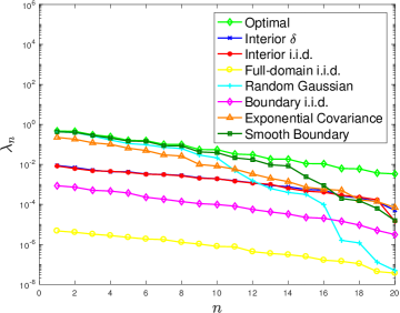
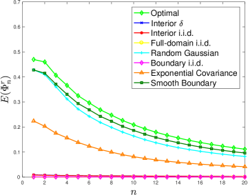
Figure 5.2. Left: Eigenvalues obtained from the six different random sampling strategies, using $20$ samples each, and the leading $20$ eigenvalues from the reference solution. Eigenvalues are computed from (3.2) for the random sampling strategies and (2.19) for the reference solution. All methods show almost exponential decay of the eigenvalues, and the Random Gaussian and the Smooth Boundary are the best two sampling strategies in the sense that they match the reference eigenvalues most closely. Right: Energy $E(\Phi_{n}^{r})$ of optimal space and approximate subspaces from different random sampling strategies using $20$ samples. Energy is computed from (4.34). Again, Random Gaussian and the Smooth Boundary strategy achieve the minimal energy gap from the optimal space.

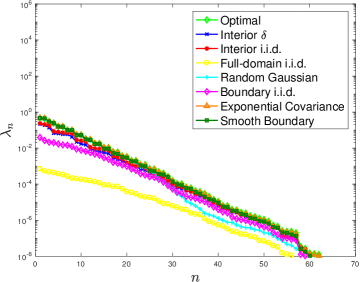
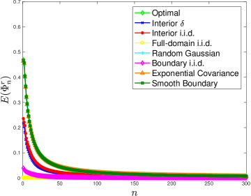
Figure 5.3. Same as Figure 5.2, but with $300$ random samples instead of $20$. Since $N_{r}\sim N_{y}$, the eigenvalues and energies obtained from random sampling tend to match the reference eigenvalues and optimal energy more closely.

Figure 5.4 shows the recovery of eigenspace by random sampling procedures. We regard $\Phi_{5}$, defined in (2.11), as the optimal space (the space expanded by the five modes with highest energies), and use $\Phi^{r}_{m}$ defined in (3.3) to approximate it, for $m=5,6,\dotsc,20$. The vertical axis shows Kolmogorov distance whose computation is described in Appendix A. As expected, using more random modes leads to better recovery and thus smaller Kolmogorov distance (4.10). The plots show Kolmogorov distance decays roughly exponentially fast with respect to $m$, for all five sampling strategies. Once again, the Random Gaussian and Smooth Boundary strategy are by far the best: $\Phi^{r}_{20}$ approximates $\Phi_{5}$ with accuracy near $10^{-4}$ or $10^{-5}$. The other four strategies attain accuracies of around $10^{-1}$ to $10^{-2}$ for $m=20$.

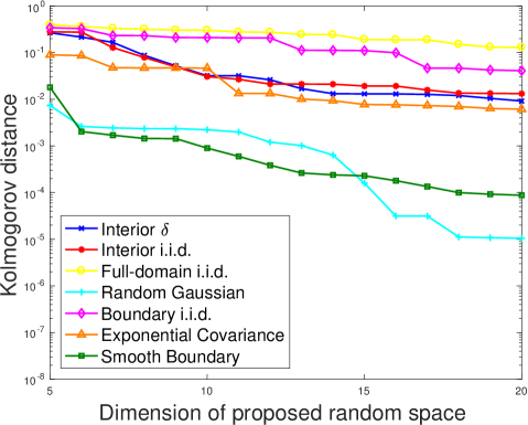
Figure 5.4. Kolmogorov distance of $\Phi_{5}$ to $\Phi^{r}_{m}$, for $m=5,6,\dotsc,20$ sampling modes.

Eigenspace Recovery for the Random Gaussian Strategy

Finally, we focus on the Random Gaussian sampling strategy, which is clearly one of the most successful strategies. In Figure 5.5, we plot in the first row the high energy modes $\{\phi_{1,2,3,4}\}$ for the reference solution, and in the second row we plot the high energy modes $\{\phi^{r}_{1,2,3,4}\}$ obtained from the Random Gaussian strategy with $20$ samples. The similarity is evident.

Figure 5.5. Recovery of high energy modes using Random Gaussian sampling strategy, with 20 samples. First row shows the first four modes of the reference solution; second row shows the first four modes obtained from the Random Gaussian sampling strategy.

6. Conclusion

In this paper we study random sampling methods that approximate the optimal solution space that attains Kolmogorov $n$-width in the context of generalized finite element methods. It is shown that certain random sampling methods capture the main part of the local solution spaces with high accuracy, and that efficiency can be evaluated by the energy contained in the proposed random space.

Numerical comparisons of seven different sampling strategies show that two strategies are superior: Random Gaussian sampling and Smooth boundary sampling.

Appendix A Calculation of the Kolmogorov Distance

Suppose we are given the optimal space

$$\Phi_{m}=\operatorname{Span}\mathsf{X},\;\mbox{where}\;\mathsf{X}=\left[\phi_{1},\ldots,\phi_{m}\right],$$

and a proposed space

$$\Phi^{r}_{n}=\operatorname{Span}\mathsf{Y},\;\mbox{where}\;\mathsf{Y}=\left[\phi^{r}_{1},\ldots,\phi^{r}_{n}\right],\quad\mbox{where $n\geq m$},$$

such that

$$\langle\phi_{i},\phi_{j}\rangle_{\mathcal{E}(\omega^{\ast})}=\delta_{ij}\quad\text{and}\quad\langle\phi_{i}^{r},\phi_{j}^{r}\rangle_{\mathcal{E}(\omega^{\ast})}=\delta_{ij}\,.$$

Recall the following definition of Kolmogorov distance from (4.10):

$${\color[rgb]{0,0,0}d(\Phi^{r}_{n},\Phi_{m})}=\max_{\begin{subarray}{c}x\in\Phi_{m},\\ \|x\|_{\mathcal{E}(\omega^{\ast})\leq 1}\end{subarray}}\,\min_{y\in\Phi^{r}_{n}}\|x-y\|_{\mathcal{E}(\omega)}\,.$$

To calculate $d(\Phi^{r}_{n},\Phi_{m})$ explicitly, we write $x=\mathsf{X}\alpha$ for some $\alpha\in\mathbb{R}^{m}$ and $y=\mathsf{Y}\beta$ for some $\beta\in\mathbb{R}^{n}$. The Kolmogorov distance is achieved when $\|x\|_{\mathcal{E}(\omega^{\ast})}=1$, which implies that $\|\alpha\|=1$, where this $\|\cdot\|$ is the usual Euclidean norm on $\mathbb{R}^{m}$. By expanding the objective, we have

$$\frac{1}{2}\|x-y\|_{\mathcal{E}(\omega)}^{2} =\frac{1}{2}\langle\mathsf{X}\alpha-\mathsf{Y}\beta,\mathsf{X}\alpha-\mathsf{Y}\beta\rangle_{\mathcal{E}(\omega)}$$

$$=\frac{1}{2}\beta^{\top}\mathsf{Y}_{A}\beta-\alpha^{\top}C_{A}\beta+\frac{1}{2}\alpha^{\top}\mathsf{X}_{A}\alpha\,,$$

where $(\mathsf{Y}_{A})_{ij}=\langle\phi^{r}_{i},\phi^{r}_{j}\rangle_{\mathcal{E}(\omega)}$, $(\mathsf{X}_{A})_{ij}=\langle\phi_{i},\phi_{j}\rangle_{\mathcal{E}(\omega)}$ and $(C_{A})_{ij}=\langle\phi_{j},\phi^{r}_{i}\rangle_{\mathcal{E}(\omega)}$. The minimizing value of $\beta$ is given explicitly by

$$\beta=\mathsf{Y}_{A}^{-1}C_{A}\alpha\,,$$

for which we have

$$\frac{1}{2}d(\Phi^{r}_{n},\Phi_{m})^{2}=\max_{\|\alpha\|=1}\alpha^{\top}(\mathsf{X}_{A}-C_{A}^{\top}\mathsf{Y}_{A}^{-1}C_{A})\alpha=\|\mathsf{X}_{A}-C_{A}^{\top}\mathsf{Y}_{A}^{-1}C_{A}\|_{2}^{2}\,.$$

The Kolmogorov distance is therefore

$$d(\Phi^{r}_{n},\Phi_{m})=\sqrt{2}\|\mathsf{X}_{A}-C_{A}^{\top}\mathsf{Y}_{A}^{-1}C_{A}\|_{2}\,.$$

Appendix B Well-posedness of energy $E(\mathcal{Z})$

We show that energy defined in Definition 4.1 is a well-defined quantity. More specifically, given a $k$-dimensional space $\mathcal{Z}$ and two different $\mathsf{B}$-orthonormal matrices $\mathsf{Z}_{1},\mathsf{Z}_{2}\in\mathbb{R}^{n\times k}$ whose columns span the space $\mathcal{Z}$, we show that they yield the same value of $E(\mathcal{Z})$:

(B.1) $$E(\mathcal{Z})=\frac{\operatorname{Tr}(\mathsf{Z}_{1}^{\top}\mathsf{A}\mathsf{Z}_{1})}{\operatorname{Tr}(\mathsf{Z}_{1}^{\top}\mathsf{B}\mathsf{Z}_{1})}=\frac{\operatorname{Tr}(\mathsf{Z}_{2}^{\top}\mathsf{A}\mathsf{Z}_{2})}{\operatorname{Tr}(\mathsf{Z}_{2}^{\top}\mathsf{B}\mathsf{Z}_{2})}\,.$$

Proof.

Since $\mathsf{Z}_{1}$ and $\mathsf{Z}_{2}$ share the column space $\mathcal{Z}$, there must exist an invertible matrix $\mathsf{P}\in\mathbb{R}^{k\times k}$ such that $\mathsf{Z}_{1}=\mathsf{Z}_{2}\mathsf{P}$.

We show first that $\mathsf{P}$ is unitary. Because both $\mathsf{Z}_{1}$ and $\mathsf{Z}$ have $\mathsf{B}$-orthonormal columns, we have

$$\mathsf{Z}^{\top}_{1}\mathsf{B}\mathsf{Z}_{1}=\mathsf{Z}^{\top}_{2}\mathsf{B}\mathsf{Z}_{2}=\mathsf{I}\,,$$

which implies that

$$\mathsf{I}=\mathsf{Z}^{\top}_{1}\mathsf{B}\mathsf{Z}_{1}=(\mathsf{Z}_{2}\mathsf{P})^{\top}\mathsf{B}(\mathsf{Z}_{2}\mathsf{P})=\mathsf{P}^{\top}\mathsf{Z}^{\top}_{2}\mathsf{B}\mathsf{Z}_{2}\mathsf{P}=\mathsf{P}^{\top}\mathsf{P}.$$

By definition of $\mathsf{Z}_{1}$ and $\mathsf{Z}_{2}$, we have

$$\frac{\operatorname{Tr}(\mathsf{Z}^{\top}_{1}\mathsf{A}\mathsf{Z}_{1})}{\operatorname{Tr}(\mathsf{Z}^{\top}_{1}\mathsf{B}\mathsf{Z}_{1})}=\frac{\operatorname{Tr}(\mathsf{Z}^{\top}_{1}\mathsf{A}\mathsf{Z}_{1})}{k},\quad\frac{\operatorname{Tr}(\mathsf{Z}_{2}^{\top}\mathsf{A}\mathsf{Z}_{2})}{\operatorname{Tr}(\mathsf{Z}_{2}^{\top}\mathsf{B}\mathsf{Z}_{2})}=\frac{\operatorname{Tr}(\mathsf{Z}^{\top}_{2}\mathsf{A}\mathsf{Z}_{2})}{k},$$

so our claim (B.1) will hold if we can show that $\operatorname{Tr}(\mathsf{Z}^{\top}_{1}\mathsf{A}\mathsf{Z}_{1})=\operatorname{Tr}(\mathsf{Z}^{\top}_{2}\mathsf{A}\mathsf{Z}_{2})$. But this follows from

$$\operatorname{Tr}(\mathsf{Z}^{\top}_{1}\mathsf{A}\mathsf{Z}_{1})=\operatorname{Tr}\left((\mathsf{Z}_{2}\mathsf{P})^{\top}\mathsf{A}(\mathsf{Z}_{2}\mathsf{P})\right)=\operatorname{Tr}\left(\mathsf{P}^{\top}\mathsf{Z}_{2}^{\top}\mathsf{A}\mathsf{Z}_{2}\mathsf{P}\right)=\operatorname{Tr}\left(\mathsf{Z}_{2}^{\top}\mathsf{A}\mathsf{Z}_{2}\mathsf{P}\mathsf{P}^{\top}\right)=\operatorname{Tr}(\mathsf{Z}_{2}^{\top}\mathsf{A}\mathsf{Z}_{2}),$$

where the last equality comes from the orthonormality of $\mathsf{P}$. ∎

References

• [1] I. Babuška and R. Lipton, Optimal local approximation spaces for generalized finite element methods with application to multiscale problems, Multiscale Model. Simul., 9 (2011), pp. 373–406.
• [2] I. Babuška and J. Melenk, The partition of unity method, International Journal for Numerical Methods in Engineering, 40 (1997), p. 727–758.
• [3] M. Bebendorf, Why finite element discretizations can be factored by triangular hierarchical matrices, SIAM Journal on Numerical Analysis, 45 (2007), pp. 1472–1494.
• [4] A. Bensoussan, J. Lions, and G. Papanicolaou, Asymptotic Analysis for Periodic Structures, AMS Chelsea Publishing Series, American Mathematical Society, 2011.
• [5] V. M. Calo, Y. Efendiev, J. Galvis, and G. Li, Randomized oversampling for generalized multiscale finite element methods, Multiscale Modeling & Simulation, 14 (2016), pp. 482–501.
• [6] W. E and B. Engquist, The heterogeneous multi-scale methods, Commun. Math. Sci., 1 (2003), pp. 87–133.
• [7] W. E, P. Ming, and P. Zhang, Analysis of the heterogeneous multiscale method for elliptic homogenization problems, J. Amer. Math. Soc., 18 (2005), pp. 121–156.
• [8] Y. Efendiev, T. Y. Hou, and X.-H. Wu, Convergence of a nonconforming multiscale finite element method, SIAM J. Numer. Anal., 37 (2000), pp. 888–910.
• [9] J. Galvis and Y. Efendiev, Domain decomposition preconditioners for multiscale flows in high contrast media: Reduced dimension coarse spaces, Multiscale Model. Simul., 8 (2010), pp. 1621–1644.
• [10] W. Hackbusch, Hierarchical Matrices: Algorithms and Analysis, Springer Series in Computational Mathematics, Springer, 2015.
• [11] N. Halko, P. G. Martinsson, and J. A. Tropp, Finding structure with randomness: Probabilistic algorithms for constructing approximate matrix decompositions, SIAM Review, 53 (2011), pp. 217–288.
• [12] T. Y. Hou and X.-H. Wu, A multiscale finite element method for elliptic problems in composite materials and porous media, J. Comput. Phys., 134 (1997), pp. 169 – 189.
• [13]  , A multiscale finite element method for pdes with oscillatory coefficients, Notes on Numerical Fluid Mechanics, 70 (1999), pp. 58–69.
• [14] T. Y. Hou, X.-H. Wu, and Z. Cai, Convergence of a multiscale finite element method for elliptic problems with rapidly oscillating coefficients, Math. Comp., 68 (1999), pp. 913–943.
• [15] T. Y. Hou and P. Zhang, Sparse operator compression of higher-order elliptic operators with rough coefficients, Research in Mathematical Sciences, (in press).
• [16] W. B. Johnson and J. Lindenstrauss, Extensions of Lipshitz mapping into Hilbert space, Contemporary Mathematics, 26 (1984), pp. 189–206.
• [17] L. Lin, J. Lu, L. Ying, and W. E, Adaptive local basis set for Kohn–Sham density functional theory in a discontinuous Galerkin framework I: Total energy calculation, J. Comput. Phys., 231 (2012), pp. 2140–2154.
• [18] R. Lipton, P. Sinz, and M. Stuebner, Uncertain loading and quantifying maximum energy concentration within composite structures, Journal of Computational Physics, 325 (2016), pp. 38 – 52.
• [19] A. Målqvist and D. Peterseim, Localization of elliptic multiscale problems, Math. Comp., 83 (2014), pp. 2583–2603.
• [20] P. Ming and X. Yue, Numerical methods for multiscale elliptic problems, J. Comput. Phys., 214 (2006), pp. 421––445.
• [21] H. Owhadi, Bayesian numerical homogenization, Multiscale Modeling & Simulation, 13 (2015), pp. 812–828.
• [22] H. Owhadi and L. Zhang, Metric-based upscaling, Comm. Pure Appl. Math., 60 (2007), pp. 675–723.
• [23] H. Owhadi, L. Zhang, and L. Berlyand, Polyharmonic homogenization, rough polyharmonic splines and sparse super-localization, M2AN Math. Model. Numer. Anal., 48 (2014), pp. 517–552.
• [24] G. Papanicolaou, Asymptotic analysis of transport process, Bull. American Math. Soc., 81 (1975), pp. 330–392.
• [25] A. Pinkus, N-widths in approximation theory, Ergebnisse der Mathematik und ihrer Grenzgebiete, Springer, 1985.