Heirarchical and synergistic self-assembly in composites of model Wormlike micellar-polymers and nanoparticles results in nanostructures with diverse morphologies.

Abstract

Using Monte carlo simulations, we investigate the self-assembly of model nanoparticles inside a matrix of model equilibrium polymers (or matrix of Wormlike micelles) as a function of the polymeric matrix density and the excluded volume parameter between polymers and nanoparticles. In this paper, we show morphological transitions in the system architecture via synergistic self-assembly of nanoparticles and the equilibrium polymers. In a synergistic self-assembly, the resulting morphology of the system is a result of the interaction between both nanoparticles and the polymers, unlike the polymer templating method. We report the morphological transition of nanoparticle aggregates from percolating network-like structures to non-percolating clusters as a result of the change in the excluded volume parameter between nanoparticles and polymeric chains. In parallel with the change in the self-assembled structures of nanoparticles, the matrix of equilibrium polymers also shows a transition from a dispersed state to a percolating network-like structure formed by the clusters of polymeric chains. We show that the shape anisotropy of the nanoparticle clusters formed is governed by the polymeric density resulting in rod-like, sheet-like or other anisotropic nanoclusters. It is also shown that the pore shape and the pore size of the porous network of nanoparticles can be changed by changing the minimum approaching distance between nanoparticles and polymers. We provide a theoretical understanding of why various nanostructures with very different morphologies are obtained.

I Introduction

Nanoparticle assembly inside a polymeric matrix is a powerful route to form hybrid materials with the desired material, magnetic, optical and electronic properties by a suitable choice of system parameters  Miyashita (2004); Black et al. (2006); Orski et al. (2011); Shenhar et al. (2005); Zhang et al. (2004); Jayaraman and Schweizer (2009); Thompson et al. (2002); Sun et al. (2002); Haryono and Binder (2006); Lin et al. (2005); Rozenberg and Tenne (2008). The synergistic interaction between nanoparticles and the polymer matrix gives rise to a variety of hybrid systems and nanostructures having a wide range of applications like in cosmetics  Arraudeau et al. (1989); Tatum and Wright (1988); Gadberry et al. (1997); Patel et al. (2006); Lochhead (2008); Corcorran et al. (2004); Laufer and Dikstein (1996); Lochhead (2007); Katz (2007); Miller (2006); Raj et al. (2012), food  Sorrentino et al. (2007); De Azeredo (2009); Rhim et al. (2013); Arora and Padua (2010); Ray et al. (2006); Sozer and Kokini (2009), pharmacy  Sambarkar et al. (2012); Ray and Bousmina (2006); Mouriño (2016); Dwivedi et al. (2013), novel functional materials  Ingrosso et al. (2010); Segala and Pereira (2012); Striccoli et al. (2009); Mazumdar et al. (2015); Carotenuto and Nicolais (2004); Qi (2017), ultraviolet lasers  Bloemer and Scalora (1998); Jakšić et al. (2004); Scalora et al. (1998); Kedawat et al. (2014), hybrid nanodiodes  Gence et al. (2010); Park et al. (2004a); Das and Prusty (2012), DNA templated electronic junctions Turberfield (2003); Park et al. (2004b), quantum dots and thin wires  Alam et al. (2013).

The investigation of nanoparticle assembly inside a polymeric matrix is important for fabrication of complex nanodevices as well as is of fundamental interest to explore the equilibrium and non equilibrium phase behaviour of the system  Dijkstra et al. (1999); Ilett et al. (1995); Lekkerkerker et al. (1992); Poon (2002); Asakura and Oosawa (1954); Aarts et al. (2002); Bolhuis et al. (2002); Gast et al. (1983). The colloid-polymer mixtures have been widely studied theoretically and experimentally and an equilibrium phase diagram is predicted using Asakura-Oosawa model  Asakura and Oosawa (1954); Lekkerkerker et al. (1992); Gast et al. (1983); De Hek and Vrij (1981); Fleer et al. (2007); Poon (2002) for their varying size ratios and volume fractions. Experimental studies confirmed the predicted equilibrium colloid-polymer phase diagram  Poon (2002); De Hek and Vrij (1981); Fleer et al. (2007) and also observed non-equilibrium phase behaviour  Poon et al. (1997). An increase in the polymer density in the colloid-polymer system leads to its demixing into two or more phases Zhang et al. (2013). In a deeply quenched system, the colloid rich phase may get kinetically arrested (on reaching the volume fraction $\approx 0.57-0.59$) during the phase separation process, suppressing the demixing and producing a non-equilibrium gel state  Zhang et al. (2013). For non-adsorbing colloid-polymer mixtures with the polymer to colloid size ratio of $\approx 0.08$, these non-equilibrium gel phases are observed for colloid volume fraction $\leq 0.3$ above a threshold of polymer concentration  Starrs et al. (2002). This limiting value of colloid volume fraction depends on polymer concentration. Above this threshold polymer concentration, these non-equilibrium phases show a period of latency (observation period over which the morphology is maintained) before sedimentation of colloids under gravity. The latency period increases with increase in the polymer concentration and may lead to ”freezing of structures” at sufficiently high concentrations  Starrs et al. (2002). Experimental studies have reported a variety of non-equilibrium phases including clusters, gels and glasses  Joshi (2014). These non-equilibrium states are a challenge for theoretical studies and forms an active area of research.

The discovery of the mesoporous material MCM-41 by Mobil Oil Corporation  Kresge et al. (1992) widely popularised the method of assembling nanostructures inside polymeric matrices and thus giving rise to the ”bottom-up” approach which revolutionised the whole industry of nanofabrication  Seul and Andelman (1995); Tang et al. (2006); Van Workum and Douglas (2006); Bedrov et al. (2005); Shay et al. (2001); Fejer and Wales (2007); Glotzer and Solomon (2007); Lee et al. (2004). Polymeric and other supramolecular matrices have long been explored as templates for fabricating nanostructures due to low cost and ease of tailoring nanomaterials with the desired properties. Later, realising the importance of synergistic interactions between nanoparticles (NPs) and the matrix, a myriad of synergistically assembled nanocomposites have also been generated. The NPs can be incorporated in a matrix by both in situ  Xu et al. (2017); Sun and Yang (2008) or ex-situ  Guo et al. (2014) methods. However, due to high surface interactions between NPs, it is difficult to disperse NPs inside the matrix. Therefore, in situ method is preferably used to produce a homogeneously dispersed NP-matrix composite. Nanorods  Luo et al. (2006); Abyaneh et al. (2016); Cao and Wang (2004), nanowires and nanobelts  Wang (2013), nanocombs and nanobrushes  Umar et al. (2008); Lao et al. (2006); Singh et al. (2010), nanosheets  Pandey et al. (2016); Vyborna et al. (2017), nanoporous  Xu (2013) and mesoporous structures  Ying et al. (1999), nanotubes, spherical and complex morphological nanostructures have been reported in the literature. However, to exploit NP properties for nanodevice fabrication, the control over their morphological structures is still a big challenge to the researchers. This paper reports transformation in the nanostructure morphology with the change in the polymeric matrix density and the excluded volume parameter between nanoparticles and polymers.

Generally, the (thermotropic) polymeric matrices have a value of elastic constants of the order of $\approx 10pN$  Sharma et al. (2009). But there exists a class of polymers known as lyotropic systems showing interesting phase behaviour due to their low value of elastic constants ($\approx 1pN$)  Ramos et al. (2000); Sallen et al. (1995). Wormlike micelles (WLM) is one of the examples of such systems. When the concentration of the surfactant molecules in presence of suitable salts becomes higher than a critical micellar concentration, the surfactant molecules then aggregate to form micelles. For appropriate shape and size of the surfactant molecules, they can aggregate into long thread-like polymeric Wormlike micelles  Berret (2006). They possess an extra mode of relaxation by scission and recombination reactions giving rise to an exponential distribution of their polymeric length  Berret (2006); Turner and Cates (1990); Cates (1990). Moreover, the average spacing of WLMs in a hexagonal H1 phase is 5-10 nm, which is much larger than that of a thermotropic polymeric matrix  Ramos et al. (2000); Sharma et al. (2009). Thus a low value of elastic constant, extra mode of relaxation and characteristic mesoscopic length scales makes the Wormlike micellar matrix different from a thermotropic polymeric matrix. In this paper, we study the hierarchical self organization of NPs in a model of self-assembling polymeric matrix that mimics the characteristic behaviour of a Wormlike micellar matrix. Our generic model of self assembling polymers represents the class of polymers known as equilibrium polymers, WLMs at mesocopic length scales are just an example of equilibrium polymers. Equilibrium polymers are those whose bond energies are order of the thermal energies $k_{B}T$, and thereby chains can break or rejoin due to thermal fluctuations.

We study the effect of the addition of NPs with diameters of the order of the diameter of equilibrium polymer (EP) chains on the polymeric self-assembly, which in turn affects the NP self-organization. The parameters which are systematically varied in our investigations are (1) the volume fractions of the polymeric matrix and (2) the minimum distance of approach between NPs and the matrix polymers (EVP - Excluded Volume Parameter). We show that for a low value of EVP, a uniformly mixed state of polymers and NPs is observed for all the densities of equilibrium polymers considered here. An increase in the value of the EVP leads to the formation of clusters of polymeric chains which joins to form a percolating network-like structure. The network of nanoparticles breaks into non-percolating clusters of NPs at some higher value of the EVP. We are able to present these morphological transformations in a diagram. There exist reports of a sudden decrease in the measured conductivity of polymer-nanocomposites in the literature  Li et al. (2010); Ambrosetti (2010). This decrease in the conductivity is attributed to the transition of NPs from non-percolating to percolating state on an decrease in NP volume fraction  Li et al. (2010); Ambrosetti (2010). In an attempt to explain these morphological transformations, we propose that these morphological transitions are due to the competition between the repulsive interaction between nanoparticles and the polymeric matrix and the repulsion between polymeric chains themselves. We try to explain this by analyzing the behaviour of total excluded volume in the system. We thus present how the system parameters can be used to tailor the mesoporous nanostructures formed in the system. This has a great potential to optimize the shape and size of nano-structures obtained by in-situ methods and there improve the design and performance of fuel cells and batteries (especially Li-ion batteries), drug delivery, optoelectronic devices and other device-properties which depend on the nano-structure morpholology.

The following section presents the potentials used to model NPs and equilibrium polymeric matrix and gives the details of the computational method. In the 3rd section, we briefly summarize our results which were published previously. In the next section, we present our new results which is divided into five sub-sections where we prove the robustness of our results and then give a detailed qualitative and quantitative analysis of the model system. We investigate the variation in EP number density and the minimum approaching distance between polymers and NPs and its effect on the system behaviour. We present our Conclusions in the last section.

II Model and method

II.1 Modeling micelles (Equilibrium Polymers)

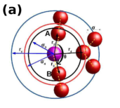
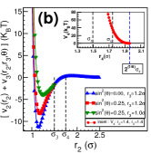
Figure 1: (colour online) (a) The figure shows the schematic representation of the range of different interactions ($V_{2},V_{3},V_{4}$) of the model potentials. The red spheres denote the monomers of size $\sigma$ which self assemble to form equilibrium polymers. All the distances are shown with respect to the monomer shown in pink. These monomers are acted upon by two body potential $V_{2}$ having a cutoff range of $r_{c}$. A three-body potential $V_{3}$ is acting on a triplet with a central monomer bonded by two other monomers (joined by a dashed line) at distances of $r_{2}$ and $r_{3}$, forming an angle $\theta$ at the central monomer (shown in pink) and having a cutoff range of $\sigma_{3}$. There is also a purely repulsive four-body potential $V_{4}$ which is a shifted Lennard-Jones potential introduced to prevent branching. The distance $2^{1/6}\sigma_{4}$ is defined as the cutoff distance for $V_{4}$. (b) The figure shows the plots of $V_{2}+V_{3}$ for different values of versus $r_{2}$ for fixed values of $\sin^{2}(\theta)$. $\sigma_{3}=1.5\sigma$ is the cutoff distance for potential $V_{3}$. The inset shows a suitably shifted Lennard-Jones potential $V_{4}$ with a cutoff distance of $2^{1/6}\sigma_{4}$, where $\sigma_{4}=1.75\sigma$.

The model we use is a modified version of a previous model presented by Chatterji and Pandit Chatterji and Pandit (2001, 2003) and also has been used in Mubeena and Chatterji (2015). In this model, WLMs are represented by a chain of beads (called monomers here which are shown as spheres in Fig.1(a)) which interact with the given potentials to form equilibrium polymers (Wormlike micelles) without branches. Each single bead or a monomer in the model is representative of an effective volume of a group of amphiphilic molecules. Thus, the WLMs are modelled at a mesoscopic scale ignoring all the chemical details. The diameter of a monomer $\sigma$ is taken as the unit of length in the system. The potential is the combination of three terms $V_{2}$, $V_{3}$ and $V_{4}$:

• We have a two body Lennard-Jones (L-J) potential modified with an exponential term.
  

  $$V_{2}=\epsilon[(\frac{\sigma}{r_{2}})^{12}-(\frac{\sigma}{r_{2}})^{6}+\epsilon_{1}e^{-ar_{2}/\sigma}];\,\forall r_{2}\leq r_{c},$$ (1)

  where $r_{2}$ is the distance between two interacting monomers with $\epsilon=110k_{B}T$ and the cutoff distance of the potential is at $r_{c}=2.5\sigma$. The exponential term in the above potential creates a maximum at $\approx 1.75\sigma$ which acts as a potential barrier for two monomers approaching each other. Two monomers are defined as bonded when the distance $r_{2}$ between them becomes $\leq\sigma_{3}=1.5\sigma$, such that the interaction energy is negative. This is explained schematically in Fig.1(a) and the plot of the potential is also shown in Fig.1(b) (full line-blue). We set $\epsilon_{1}=1.34\epsilon$ and $a=1.72$.

• To model semiflexibility of chains, we use a three-body potential $V_{3}$,

  $$V_{3}=\epsilon_{3}(1-\frac{r_{2}}{\sigma_{3}})^{2}(1-\frac{r_{3}}{\sigma_{3}})^{2}\sin^{2}(\theta);\,\forall r_{2},r_{3}\leq\sigma_{3}.$$ (2)

  Here $r_{2}$ and $r_{3}$ are the distances of the two monomers A and B (refer Fig.1(a)) from the central monomer (coloured pink) which forms a triplet with an angle $\theta$ subtended by $\vec{r_{2}}$ and $\vec{r_{3}}$. Here $\epsilon_{3}=6075k_{B}T$. The prefactors to $\sin^{2}(\theta)$ are necessary to ensure that the potential and force goes smoothly to zero at the cutoff distance $\sigma_{3}=1.5\sigma$ for $V_{3}$. This three-body potential modeling semiflexibility acts only if a monomer has two bonded neighbors at distances of $\leq\sigma_{3}$. Fig.1(b) shows the plots of $V_{2}+V_{3}$ for $r_{2}=\sigma$ and different values of $r_{3}$ and $\theta$. This potential penalizes angles $<180^{\circ}$. Configurations with $\theta=0^{circ}$ are prevented by excluded volume interactions of the monomers.

• Monomers interacting by potentials $V_{2}$ and $V_{3}$ self-assemble to form linear polymeric chains with branches. A fourth monomer can get bonded with a monomer which already has two bonded neighbours to form a branch. To avoid branching, it is necessary to repel any monomer which can potentially form a branch. Therefore, we introduce a four-body potential term which is a shifted Lennard-Jones repulsive potential $V_{4}$ which repels any branching monomer at distances $\approx\sigma_{4}$, where $\sigma_{4}=1.75\sigma>\sigma_{3}$. The explicit form of the potential $V_{4}$ is,

  $$V_{4}=\epsilon_{4}(1-\frac{r_{2}}{\sigma_{3}})^{2}(1-\frac{r_{3}}{\sigma_{3}})^{2}\times V_{LJ}(\sigma_{4},r_{4});\forall r_{4}\leq 2^{1/6}\sigma_{4}$$ (3)

  Here $r_{2}$ and $r_{3}$ are the distances of the two monomers from central monomer(coloured pink) which forms a triplet, while $r_{4}$ is the distance of the fourth monomer which tries to approach the central monomer which already has two bonds, as shown in Fig. 1(a). We set the cutoff distance for this potential to be $2^{1/6}\sigma_{4}$ with a large value of $\epsilon_{4}=2.53\times 10^{5}k_{B}T$. The value of $\epsilon_{4}$ is kept large enough to ensure enough repulsion in case $(1-\frac{r_{2}}{\sigma_{3}})^{2}<<1$ and/or $(1-\frac{r_{3}}{\sigma_{3}})^{2}<<1$. These terms are necessary to ensure that if $r_{2}$ or $r_{3}$ becomes $\geq\sigma_{3}$, $V_{4}$ and the corresponding force goes smoothly to zero at the cutoff of $\sigma_{3}$.

All the three potentials are summarised in Fig.1(a). In this figure, the red spheres denote the micellar monomers having size $\sigma$. These monomers are acted upon by two body potential $V_{2}$ having a cutoff range of $r_{c}$. The potential is shown in Fig.1(b) indicated by the legends $\sin^{2}\theta=0$ (triangle-blue line). A three-body potential $V_{3}$ is acting on a triplet with a central monomer bonded by two other monomers at distances $r_{2}$ and $r_{3}$ (bonded monomers are joined by dashed lines). The vectors $\vec{r_{2}}$ and $\vec{r_{3}}$ subtends an angle $\theta$ at the central monomer and the potential $V_{3}$ has a cutoff distance of $\sigma_{3}$ (Fig.1(b)). The three-body potential $V_{3}$ modifies the two body potential $V_{2}$ such that the resultant potential energy $V_{2}+V_{3}$ gets shifted to a higher value of energy depending on the value of $\theta$, $r_{2}$ and $r_{3}$. This is illustrated in the graph for $\sin^{2}\theta=0.25$ and two different values of $r_{3}=1.2\sigma$ and $\sigma$ keeping the value of $r_{2}$ fixed at $r_{2}=\sigma$. For a given value of $\theta$, the potential energy $V_{2}+V_{3}$ is lower for higher value of $r_{3}$. In addition to $V_{2}$ and $V_{3}$, there is also a four-body potential $V_{4}$ which is a shifted Lennard-Jones potential introduced to prevent branching and having a cutoff distance $2^{1/6}\sigma_{4}$. The behaviour of potential energy $V_{4}$ is shown in the inset of Fig.1(b). The vertical lines indicate $\sigma_{3}=1.5\sigma$ and $\sigma_{4}=1.75\sigma$. The vertical line (in blue) in the inset figure shows the cutoff distance of $V_{4}$ at $2^{1/6}\sigma_{4}$.

II.2 Modeling Nanoparticles

To explore the self-organization of NPs inside Wormlike micellar matrix (or EP matrix), we need to introduce a suitable model for NPs. The NP-NP interactions are modelled by a Lennard-Jones potential for particles of size $\sigma_{n}$,

$$V_{2n}=\epsilon_{n}[(\frac{\sigma_{n}}{r_{n}})^{12}-(\frac{\sigma_{n}}{r_{n}})^{6}],\forall r_{n}\leq r_{cn}$$ (4)

where, ${r_{n}}$ is the distance between the centres of two interacting NPs. The potential $V_{2n}$ goes smoothly to zero at the cutoff distance $r_{cn}=2\sigma_{n}$. The interaction between NPs and micellar monomers at a distance r is modelled by a repulsive WCA (Weeks-Chandler-Anderson) potential given by,

$$V_{4n}=\epsilon_{4n}[(\frac{\sigma_{4n}}{r})^{12}-(\frac{\sigma_{4n}}{r})^{6}],\forall r\leq 2^{1/6}\sigma_{4n},$$ (5)

The strength of attraction for the above potential is kept to be $\epsilon_{4n}=30k_{B}T$. The value of $\sigma_{4n}$ here defines the minimum approaching distance between a NP and a monomer. Therefore, it is used as EVP between micelles and NPs. Since the monomers and NPs of diameters of $\sigma$ and $\sigma_{n}$ are considered to be nearly impenetrable, the EVP cannot be less than $\sigma/2+\sigma_{n}/2$. Thus, there exists a lower bound for the variable $\sigma_{4n}$ and it can only have values $\sigma_{4n}\geq\sigma/2+\sigma_{n}/2$. This is explained in Fig.2. In summary, the model has a fixed value of monomer diameter $\sigma$ and NP diameter $\sigma_{n}$ ($=1.5\sigma$) with the minimum approaching distance between them $\sigma_{4n}$ used as a variable along with monomer number density $\rho_{m}$ . All the other values are kept constant. The polymeric matrix thus modelled is equally applicable for a Wormlike micellar matrix or any other equilibrium polymeric matrix.

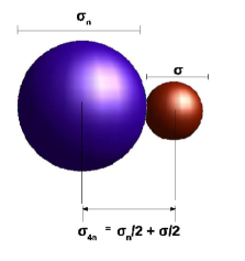
Figure 2: The figure is a schematic diagram to explain the role of the parameter $\sigma_{4n}$ by which we control the excluded volume of the monomers when they interact with nan-particles. The parameter $\sigma_{4n}$ is shown as the minimum approaching distance between nanoparticles and monomers and calculated as $\sigma_{4n}=\sigma/2+\sigma_{n}/2$. For monomers of diameter $\sigma$ and nanoparticles of diameter $\sigma_{n}=1.5\sigma$, the minimum allowed value of $\sigma_{4n}$ is $(\sigma_{4n})_{min}=1.25\sigma$. We use $\sigma_{4n}$ as a parameter and we choose values $\sigma_{4n}\geq 1.25\sigma$ keeping $\sigma_{n}=1.5\sigma$ fixed.

II.3 Method

To study the system behaviour, we randomly place model monomers and NPs with a fixed volume fraction in a box of size $V=30\times 30\times 60\sigma^{3}$ with periodic boundary conditions where the unit of energy is set by choosing $k_{B}T=1$. We used Monte Carlo method (Metropolis algorithm) to evolve the system towards equilibrium. For a high-density regime, the Metropolis Monte Carlo moves seemed to be inefficient to equilibrate the system. Therefore, the system is first allowed to equilibrate for $10^{5}$ iterations with a few (100-200) NPs inside it so that monomers can self-assemble in the form of chains in the presence of the seeding of NPs. Once the chains are formed in the presence of seeded NPs ($~{}10^{5}$ iterations) then, a semi-grand canonical Monte Carlo (GCMC) scheme is switched on for the rest of the iterations. According to this scheme, every 50 Monte Carlo Steps (MCSs), 300 attempts are made to add a NP at a random position or remove a randomly chosen NP in the system. Each successful attempt of adding or removing a NP is penalised by an energy gain or loss of $\mu_{n}$, which sets the chemical potential of NP system. A higher value of $\mu_{n}$ leads to the lower number of NPs getting introduced in the system. The system is evolved with the GCMC scheme for $2\times 10^{6}$ to $4\times 10^{6}$ iterations and the thermodynamic quantities considered are averaged over ten independent runs. For the lowest value of $\sigma_{4n}$ used, i.e. $\sigma_{4n}=1.25\sigma$, a rapid introduction of a large number of NPs into the box was observed as soon as GCMC was switched on. This led to a large number of NPs ($\approx 10^{4}$ or more) in the simulation box and shorter runs. After the number of NPs in the simulation box had relatively stabilized, the acceptance rate of of GCMC attempts was $\sim 5\%$, with a slightly lower rate of removal of NPs from the simulation box, which resulted in a net $~{}0.1\%$ addition of particles in the box. For the higher values of $\sigma_{4n}$, the rate of GCMC acceptance is $10-20\%$ and also reaches to $30\%$ in case of $\sigma_{4n}=3.5\sigma$. Similarly, the acceptance rate of attempts to remove NPs also remains approximately same resulting in the net $0.02-0.07\%$ rate of addition of NPs. The rate with which NPs are added decreases with increase in $\sigma_{4n}$.

III Previous results

In our previous communication  Mubeena and Chatterji (2015), we used the same model potentials described here to show that monomers interacting with the potentials self-assemble to form long cylindrical chains akin to WLMs. These polymeric chains show an exponential distribution of chain length, thus, confirming the characteristic behaviour of equilibrium polymer (or Wormlike micellar) matrix  Turner and Cates (1990). The self-assembled polymers at low densities were observed to be in a disordered (isotropic) state with relatively small chains. With an increase in the monomer number density, the short chains or monomers start joining up to form longer chains. These chains then start getting parallel to neighbouring chains, and the system shows a transition to a nematically ordered state at a high value of density. We observe a isotropic to nematic first order transition at monomer number density $\rho_{m}\approx 0.13\sigma^{-3}-0.14\sigma^{-3}$.

The behaviour of the mixture of the model NPs and equilibrium polymeric chains was investigated at a high monomer number density $\rho_{m}=0.126\sigma^{-3}$ with the change in $\sigma_{4n}$. The kinetically arrested assembly of NPs shows a transition from a system spanning percolating network-like structure to non-percolating clusters with an increase in EVP ($\sigma_{4n}$). The clusters of NPs were observed to be having rod-like structures.

IV Present investigation

In this paper, the self-assembly of the equilibrium polymeric chains + NP system is investigated as a function of the $\sigma_{4n}$ (EVP) and $\rho_{m}$. Throughout the paper, the diameter of NPs $\sigma_{n}$, the quantity $\sigma_{4}$ and the NP chemical potential are kept fixed at $1.5\sigma$, $1.75\sigma$ and $-8k_{B}T$, respectively, unless otherwise mentioned. All the distances mentioned here refer to the centre-to-centre distances of the particles involved. To investigate the behaviour of NPs and wormlike micellar system, four different values of the number of monomers $N_{m}$ are considered viz. $N_{m}=2000$, $4000$, $5000$ and $6800$ corresponding to the monomer number densities $\rho_{m}=0.037\sigma^{-3},0.074\sigma^{-3}$, $0.093\sigma^{-3}$ and $0.126\sigma^{-3}$, respectively.

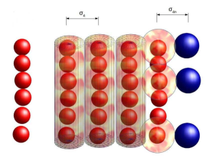
Figure 3: (colour online) The figure explains the calculation of the effective volume of monomers. Red colored particles represents monomers, whereas the nanoparticles are shown in blue. Two neighbouring polymeric chains with distance between monomers centers $<\sigma_{4}=1.75\sigma$ are considered as the cylinders of radius $\sigma_{4}$. Monomers whose position is within the range $2^{1/6}\sigma_{4n}$ of repulsive potential $V_{4n}$ are assumed as spheres of radius $(\sigma_{4n}-\sigma_{n}/2)$, where $\sigma_{n}$ is the radius of nanoparticles.

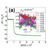
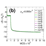
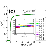
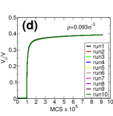
Figure 4: (colour online) The subplots (a),(b) shows the plots of average energy per particle (both monomers and NPs) for two different values of monomer number density $\rho_{m}$. The subplots (c),(d) shows nanoparticle volume fraction $V_{n}/V$ versus MCSs, $V_{n}$ is the volume of NPs and $V$ is the volume of simulation box. The parameter $\sigma_{4n}$ is kept fixed at $1.25\sigma$. Each figure shows multiple graphs generated from $10$ independent runs initialized with different initial configurations which can be clearly seen in the magnified parts of the graphs shown in the inset of figures (a) and (c). The system is evolved with MC steps for a first $10^{5}$ iterations and then subjected to the grand-canonical MC (GCMC) scheme on nanoparticles. The data show a sudden jump in their values when we switch on GCMC.

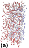
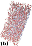
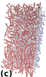
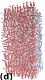
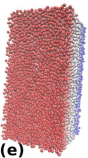
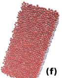
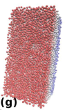
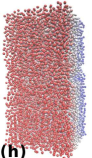
Figure 5: (colour online) The upper row of snapshots shows snapshots of only the equilibrium polymers (micellar chains) and the lower row shows only the nanoparticles of the NP+polymer system. Different snapshots are for different values of monomer densities; (a),(e) is for $\rho_{m}=0.037\sigma^{-3}$, (b),(f) is for $\rho_{m}0.074=\sigma^{-3}$, (c),(g) is for $\rho_{m}=0.093\sigma^{-3}$ and (d),(h) is for $\rho_{m}0.126\sigma^{-3}$. The value of $\sigma_{n}$ and $\sigma_{4n}$ is kept fixed at $1.5\sigma$ and $1.25\sigma$, respectively. All the snapshots show that the nanoparticle-monomer system are in uniformly mixed state and clustering of micellar chains is not observed. All the figures have a gradient in their colour varying from red to blue to identify and distinguish between the particles which are near the front plane (red) and the ones which are closer to the the back of the box (blue).

IV.1 Calculation of effective Volume

We realize that the system behaviour can be better characterized by considering the total excluded volume of clylindrical polymer chains and NPS due to the repulsive interactions $V_{4}$ and $V_{4n}$ instead of only considering the volume fraction of spherical monomers. We define the total volume excluded by a chain due to the repulsive potentials from $V_{4}$ and and $V_{4n}$ as the effective volume of the chain. The effective volume of a monomer is the effective volume of the chains divided by the total number of monomers. The calculation of the effective volume of WLMs is explained in Fig.3. The figure shows that any two micellar chains (red spheres) at a distance of the cutoff distance ($2^{1/6}\sigma_{4}$) (range of the repulsive interaction ($V_{4}$)) from each other are considered as non-overlapping cylinders of diameter $\sigma_{4}$ (shaded cylinders). Correspondingly, the effective volume of the monomer in the chain is defined to be $v_{1}=\pi(\sigma_{4}/2)^{2}\sigma$. If a monomer is at a distance less than the cutoff distance $2^{1/6}\sigma_{4n}$ (for $V_{4n}$) from a nanoparticle, then the monomer is considered to be a sphere of radius $(\sigma_{4n}-\sigma_{n}/2)$ (shaded sphere) and the effective volume of the monomer is $v_{2}=4\pi/3(\sigma_{4n}-\sigma_{n}/2)^{3}$. Any monomer that is not involved in any of the repulsive interactions $V_{4}$ and $V_{4n}$ has the volume $v_{3}=4\pi/3(\sigma/2)^{3}$.

To calculate this effective volume using a suitable algorithm, first, we identify and label the monomers which are part of a chain. All monomers within a distance of $1.5\sigma$ (cutoff distance for $V_{3}$) from each other are considered as bonded and thus form part of a chain. We do not observe branching in the chains. Then all the chains that are involved in the repulsive interactions from other chains or nanoparticles are identified and the effective volume of micelles is calculated according to the scheme discussed above and illustrated in Fig.3. If a monomer interacts with a monomer of a neighbouring chain as well as a NP simultaneously, then, the higher of the two values of effective volume ($v_{1}$ or $v_{2}$) is considered. The effective volume fraction of micelles, thus calculated, depicts the actual excluded volume fraction because of the repulsive potentials $V_{4}$ and $V_{4n}$ in addition to the volume fraction of monomers ($\rho_{m}4/3\pi(\sigma/2)^{3}$). If there are $n_{1}$ monomers interacting with other monomers with potential $V_{4}$, $n_{2}$ monomers having repulsive interaction $V_{4n}$ with a nanoparticle and $n_{3}$ monomers out of range of the potentials $V_{4}$ and $V_{4n}$ then, $n_{1}v_{1}+n_{2}v_{2}+n_{3}v_{3}$ depicts the effective volume of micelles. This effective volume of monomers is not only dependent upon the value of $\sigma_{4}$ and $\sigma_{4n}$ but also on the arrangement of the constituent particles. The effective volume thus calculated will help in understanding the behaviour of the system. For monomers situated in between a micellar chain and NPs, the volume may get slightly overestimated when $\sigma_{4n}-\sigma_{n}>\sigma_{4}$. This is because of the over-calculation of the volume in case of overlapping of the shaded (red) spheres and shaded monomer chains (cylinders) as shown in the Fig.3. However, this overestimation does not change the interpretation of results.

IV.2 Investigation for systems with $\boldsymbol{(\sigma_{4n})_{min}=1.25\sigma}$: Formation of a dispersed state of polymeric chains

$\boldsymbol{{{{\rho_{m}=0.037\sigma^{-3}}}}}$                                     $\boldsymbol{{{{\rho_{m}=0.126\sigma^{-3}}}}}$
$\overbrace{\boldsymbol{initial}\hskip 28.45274pt\rightarrow\hskip 28.45274pt\boldsymbol{final}}$                   $\overbrace{\boldsymbol{initial}\hskip 28.45274pt\rightarrow\hskip 56.9055pt\boldsymbol{final}}$
                                                                                          $\overbrace{\mu_{n}=-8k_{B}T\hskip 28.45274pt\mu_{n}=4k_{B}T}$

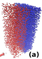
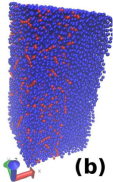
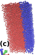
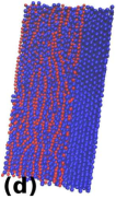
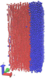
Figure 6: (colour online) The figure shows the snapshots of the system for monomer number densities $\rho_{m}=0.037\sigma^{-3}$ (figures (a) and (b)) and $0.126\sigma^{-3}$ (figures (c), (d) and (e)). Red particles indicate monomers while nanoparticles are shown in blue. For each $\rho_{m}$, the two snapshots in (a) and (c) represent the initial configuration of monomers and NPS, where NPs and monomers are kept on two sections of the simulation box. The snapshots in (b) and (d) show the microstates after $4\times 10^{6}$ iterations (with GCMC switched on after $10^{5}$ iterations). In both the cases of densities, the final state deviates from the initial state forming a uniformly mixed states of micellar chains + nanoparticles, this coexists with a state which occupies part of the box which has only densely packed nanoparticles (without micellar chains). The snapshot in figure (e) shows the final state of the system initialized as in (c) but with a higher value of chemical potential $\mu_{n}=4k_{B}T$. The states reached after the runs for $\mu_{n}=-8k_{B}T$ (figure (d)) and $\mu_{n}=4k_{B}T$ (figure (e)) are different. The state in (e) shows a phase separated state.

To study the effect of change of micellar density, the system is simulated with different monomer number densities at $\sigma_{4n}=1.25\sigma$ (minimum allowed value of $\sigma_{4n}$; refer Fig.2). To check the robustness of the results, for each number density of monomers, the system is observed over ten independent runs each starting with different initial random configurations. First, the system is evolved by applying Monte Carlo technique for $10^{5}$ iterations and then GCMC scheme is switched on for the rest of the iterations. Fig.4 shows the evolution of the average energy of the constituent particles ($\langle E\rangle$) and the NP volume fraction $V_{n}/V$ with MCSs, for two different values of monomer number densities. The NP volume $V_{n}$ is given by $V_{n}=N_{n}4/3\pi{\sigma_{n}}^{3}$ where, $N_{n}$ is the number of NPs in the simulation box. Both the figures for energy per unit constituent particle (Fig.4(a) and (b)) and the volume fraction of NPs graphs (Fig.4(c) and (d)) show data for multiple runs generated from 10 independent runs. All these graphs from different independent runs overlap and look indistinguishable from each other. Therefore, magnified parts of the graphs are shown in the insets of figures (a) and (c). in the number of NPs with MCS. The inset figures clearly show different graphs for different independent runs indicated by different colours, for a small range of iterations. All the graphs show a jump on switching to the GCMC scheme at $10^{5}$ of MCSs, indicating an increase in the NP volume fraction in the system. The insets clearly show the energy fluctuations and gradual increase in the number of NPs with MCS.

All the independent runs for each $\rho_{m}$ produce similar configurations after (2 to 4)$\times 10^{5}$ iterations and the energy and NP volume fraction graphs converge to the same value. For each $\rho_{m}$, a very long run (  $4\times 10^{6}$ iterations) was given to check if there is any change in the morphology of the system within thermal fluctuations. The system is found to maintain its morphology across all independent runs. After $\approx 2\times 10^{5}$ iterations, the system morphology remains relatively unchanged for the length of the runs varying from $4\times 10^{5}$ to $4\times 10^{6}$ of iterations. Once the energy graphs show a very slow variation in its values and no further change in the polymer-NP morphology is observed, we show the representative snapshots for each of the monomer number densities $\rho_{m}$ in Fig.5. The monomers and the NPs are shown separately in the upper row and the lower row, respectively. All the snapshots have a gradient in colour varying from red (front plane) to blue (rear plane) along one of the box lengths, for a better visualisation of a three-dimensional figure. The figure shows the snapshots for (a) $\rho_{m}=0.037\sigma^{-3},(b)0.074\sigma^{-3},(c)0.093\sigma^{-3}$ and (d) $0.126\sigma^{-3}$. No clustering of micellar chains is observed, i.e. any two neighbouring chains are always found with NPs in between. In other words, the NP-monomer system forms a uniformly mixed state.

An increase in the nematic ordering of polymeric chains and their chain length can be recognized from the figures as a result of the change in $\rho_{m}$ in Fig.5. The snapshot in Fig.5(a) shows smaller chains in a disordered state and the chain length and order increases for Figs.5(b) and 5(c) and finally the system forms a nematic state with longer and aligned chains in Fig.5(d). All the systems shown in the figure may show different polymer arrangements, but for all the micellar densities a uniformly mixed state of polymeric chains and NPs is observed.

All the independent runs discussed till now had the systems initialized in a state where the positions of both the monomers and 200-300 seed nanoparticles are randomly chosen. To ensure that our conclusions are not dependent on initial conditions, we gave additional runs initialized with all monomers on one side and all the NPs on the other side of the box. The representative snapshots from these runs after $4\times 10^{6}$ iterations, for $\rho_{m}=0.037\sigma^{-3}$ [Fig.6(a) and (b)] and $\rho_{m}=0.126\sigma^{-3}$ [Fig.6(c), (d) and (e)] are shown. Figure 6(a) [and (c)] shows the initial state with $\rho_{m}=0.037\sigma^{-3}$ with $N_{m}=2000$ [$\rho_{m}=0.126\sigma^{-3}$ with $N_{m}=6800$] and 5000 [5000] NPs in the box. Figures 6 (b) and (d) show the snapshots after $4\times 10^{6}$ MCSs for systems initialized as shown in Figs. (a) and (c), respectively. The Fig.6(e) shows the snapshot initialized with the same configuration shown in (c) but having the value of $\mu_{n}=4k_{B}T$. For both the densities of monomers considered for $\mu=-8k_{B}T$, the final state is different from the initial state forming a uniformly mixed state of monomer chains and NPs (left side of the box) coexisting with NPs without monomers (right side of the box) (figures (b) and (d)). The runs were tested with different initial numbers of NPs, but all the runs resulted in a mixed state of polymeric chains and NPs (as shown in the left part of the boxes in Figs.6(b) and 6(d)). These mixed states are found to be coexisting with NPs shown in the right sides of the boxes. We expect that if the system reaches equilibration, the systems will evolve to a completely mixed state as in Figs.5(e), (f), (g) and (h) for $\sigma_{4n}=1.25\sigma$ and $\mu_{n}=-8k_{B}T$. But in our studies, the density of monomers and NPs are locally very high, which leads to very packed structures which is unable to relax to equilibrium. However, keeping the initial state similar to Fig.6(c) and increasing the value of $\mu_{n}$ from $\mu_{n}=-8k_{B}T$ to $\mu_{n}=4k_{B}T$ for $\rho_{m}=0.126\sigma^{-3}$ resulted in a phase separated state as shown in Fig.6(e).

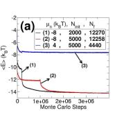
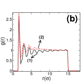
Figure 7: (colour online) (a) The figure compares the average potential energy $\langle E\rangle$ of the constituent particles (monomers and NPs) versus MCSs of the systems that are initialized as shown in Fig.6(c). Lines (1) and (2) correspond to data with $\mu_{n}=-8k_{B}T$ and line (3) corresponds to data with $\mu_{n}=4k_{B}T$. The graphs (2) and (3) corresponds to the systems represented in Figs.6(d) and (e), respectively, at the end of the run. The graphs (1) and (2) differs in their number of nanoparticles in the initial configuration $N_{init}$ as well as in the value of iterations/MCS after which the GCMC scheme is switched on. The two graphs (1) and (2) illustrates that the results are independent of the value of $N_{init}$ and the number of iterations after which the GCMC scheme is switched on, as for both cases $\langle E\rangle$ converges to the same value within statistical fluctuations. On switching on to GCMC scheme, graphs (1) and (2) jumps to a lower value of $\langle E\rangle$. This is indicative of the rapid addition of nanoparticles in the system. The line (3) jumps to a slightly higher value of energy indicating the removal of nanoparticles. The legends $N_{f}$ indicates their final value of the number of nanoparticles after $4\times 10^{6}$ MCS. (b) The figure shows the pair correlation function $g(r)$ for the NPs in left two-thirds of the box represented by line-2 and the NPs in the right one-third of the box (line-1) corresponding to the configuration shown in the Fig.5(d). The pair correlation function shows the presence of a long-range correlations in the position of NPs corresponding to a crystalline ordered state in the right section of the box.

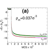
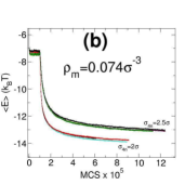
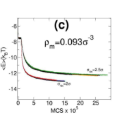
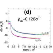
Figure 8: (colour online) Plots of average potential energy $\langle E\rangle$ per particle (monomer and NP) of the system for different values of monomer number densities (a) $\rho_{m}=0.037\sigma^{-3},(b)0.074\sigma^{-3},(c)0.093\sigma^{-3}$ and (d) $0.126\sigma^{-3}$. Each figure shows the energy graphs for two different values of $\sigma_{4n}=2\sigma$ and $2.5\sigma$. For each value of $\sigma_{4n}$, there are ten graphs overlapping each other and converging to the same values. The Monte Carlo scheme (without GCMC) is applied for first $10^{5}$ iterations. Then the GCMC scheme is switched on which leads to a further decrease in the energy values indicated by jumps in the values of $\langle E\rangle$ in each graph.

Thus, it is observed that for $\mu_{n}=-8k_{B}T$, the system initialized as shown in Fig.6(c) always leads to form a mixed state while, for $\mu_{n}=4k_{B}T$, the system remains in a phase separated state. This difference in the behaviour of the systems with different values of $\mu_{n}$ can be confirmed by the plots shown in Fig.7(a). The figure shows three graphs (1), (2) and (3). For all the graphs the state of initialization is as shown in Fig.6(c) but with a different initial number of nanoparticles $N_{init}$ as indicated in the figure. Graphs (1) and (2) shows the evolution of energy with MCSs for $\mu_{n}=-8k_{B}T$ initialized with 2000 and 5000 NPs, respectively. Both the graphs show convergence to the same value of energy after $4\times 10^{6}$ iterations with a jump to lower energy values on switching on the GCMC scheme at $10^{5}$ and $10^{6}$ iterations, respectively. This jump to lower energy indicates the addition of NPs into the box on switching on the GCMC scheme. Irrespective of (i) the number of MCSs at which the GCMC scheme is switched on and (ii) the initial number of NPs $N_{init}$, all the systems are observed to evolve to form a mixed state and converges to the same value of energy for $\mu_{n}=-8k_{B}T$ (two of which constitutes the graphs (1) and (2)). Graph (3) shows the evolution of energy for the system initialized with the same state as in Fig.6(c) with 5000 NPs in the box, but having a higher value of $\mu_{n}=4k_{B}T$. On switching on the GCMC scheme, the graph shows a jump at $10^{5}$ MCSs to a higher value of energy indicating removal of NPs from the box. The system evolves to form an equilibrated phase separated state as shown in 6(e) after removal of $\approx 550$ NPs from the box. Since all the systems initialized with the configuration shown in 6(c) and $\mu_{n}=-8k_{B}T$ evolves to form a mixed state irrespective of the initial number of NPs in the system, it can be concluded that for $\mu_{n}=-8k_{B}T$, a phase separated state is not a thermodynamically preferred state. Therefore, we can now claim from the snapshots shown in Fig.5 that the mixed state will remain the thermodynamically preferred state as well, for $\sigma_{4n}=1.25\sigma$. We remind the reader that we do not claim that the microstates corresponding to the the snapshots of Fig.5 are in equilibrium that the values of both the average energy as well $V_{n}/V$ are evolving.

For the value of $\mu_{n}=-8k_{B}T$, one more difference can be observed for different values of $\rho_{m}$ which can be seen in Figs.6(b) and 6(d). Both the figures are initialized with similar configurations (unmixed state) and number of NPs $N_{init}=5000$, but with different values of monomer number density $\rho_{m}=0.037\sigma^{-3}$ [Fig.6(a)] and $\rho_{m}=0.126\sigma^{-3}$ [Fig.6(c)]. In case of higher density of monomers, the phase of NPs which is devoid of monomers (in the right part of the box in Fig.6(d)) seems to have a long-range crystalline order compared to the lower density case [refer the right part of the box in Fig.6(b)]. The figure 7(b) compares the pair correlation function for the NPs in left section box in Fig.6(d) as well as the right section where the NPs dont have monomers interspersed between them. The correlation graphs for NPs in the mixed state (in the left part of the box in Fig.6(d)) depicted in graph (2) shows very few and low peaks which die out quickly compared to the graph for NPs (in the right part of the box of Fig.6(d)) as depicted by graph (1). The graph (1) has very sharp peaks and shows a longer range of correlation hence, confirming the observed ordered structure of NPs. We expect that these two coexisting states as shown in Fig.6(b) and (d) are stuck in a metastable state and they will form a fully mixed state after equilibration.

All the results for ten independent runs and the runs shown in Fig.6 indicate that the mixed state of NP and micellar chains could be the thermodynamically preferred state of the system for the value of $\mu_{n}=-8k_{B}T$. The systems considered here are quite dense and show a very slow increase in the number of nanoparticles even after a very long run (Fig.8(c,d)). Therefore, we assume that the structures discussed in the previous sections (see Fig.5) are most probably kinetically arrested states that are relaxing slowly to equilibrium. The rest of the paper considers the systems initialized with a randomly mixed state of micelles and NPs and investigates the effect of the change in $\sigma_{4n}$ for each value of $\rho_{m}$.

IV.3 $\sigma_{4n}>1.25\sigma$: Polymer and NP clusters with different morphologies

We next investigate the effect of the change in the value of $\sigma_{4n}$ for different monomer densities by varying $\rho_{m}$ and $\sigma_{4n}$. The results from these runs were further substantiated with ten independent runs for each value of $\rho_{m}$ and $\sigma_{4n}$. The average energy of the system for ten independent runs for two different values of $\sigma_{4n}=2.5\sigma$ and $2\sigma$ is shown in Fig.8 for values of densities (a) $0.037\sigma^{-3},(b)0.074\sigma^{-3},(c)0.0931\sigma^{-3}$ and $(d)0.126\sigma^{-3}$. The system is evolved with Monte Carlo steps without GCMC for the first $10^{5}$ iterations and then the GCMC scheme is switched on which is marked by a rapid lowering in the energy values in Fig.8. This lowering of energy values corresponds to the rapid addition in the number of nanoparticles in the system but, the rate of addition slows down after $(2-5)\times 10^{5}$ iterations. In each figure, each visible line shows multiple lines overlapping each other, generated by ten independent runs. All the ten independent runs converge to the same value of energy. Here, we would like to emphasise again that all the systems are initialized with random positions of monomers and 200-300 seed nanoparticles and with the grand-canoninal Monte Carlo steps NPs get introduced in the midst of the micellar chains. This method of initialization is a reminiscent of the in situ method of preparation of nanoparticles inside the matrix of polymers, where the NPs start nucleating out from a chemical solution on suitable addition of a reactant.

After evolving the system for $(2-4)\times 10^{6}$ iterations, the representative snapshots for four different values of $\rho_{m}=0.037\sigma^{-3}$, $0.074\sigma^{-3}$, $0.093\sigma^{-3}$ and $0.126\sigma^{-3}$ are shown in figures 9, 10, 11 and 12, respectively. For each NP+micelles system, the monomers and NPs are shown separately in the upper and lower rows, respectively, in figures 9, 10, 11 and 12. Each figure shows the snapshots for four different values of $\sigma_{4n}$ increasing from (a) to (d) for monomers (in red) (or (e) to (h) for NPs in blue). Only for snapshots of NPs in Figs.9, 10(a) and 10(e), there exists a gradient in colour (varying from red to blue along one of the length of the simulation box) from front plane to the rear plane. This helps to identify particles lying in different planes and thereby clearly see the pores in NP aggregates. These pores are occupied by monomers.

In each of the figures, one can see in the leftmost snapshot (snapshots (a) and (e), which are for a lower value of $\sigma_{4n}$) a network-like structure of micellar chains or NPs which spans the system. An increase in the value of $\sigma_{4n}$ leads to a decrease in number of nanoparticles that gradually breaks the network connections, thus, gradually breaking the network of NPs as shown in Figs.10(g), 11(f,g) and 12(f). With further increase in $\sigma_{4n}$, these networks break into non-percolating clusters as shown for $\sigma_{4n}=3.25\sigma,3\sigma$ and $2.25\sigma$ in figures 10(h), 11(h) and 12(g), respectively. We do not observe the breaking of networks into individual NP clusters for $\rho_{m}=0.037\sigma^{-3}$ in Fig.9 for the range of values of $\sigma_{4n}$ considered here. Therefore with an increase in $\rho_{m}$, the value of $\sigma_{4n}$ at which the network breaks into non-percolating clusters gets shifted to a lower value of $\sigma_{4n}$. From the snapshots 10(h), 11(h) and 12(g), it can be clearly seen that different densities of micelles lead to different shape-anisotropy of nanoparticle clusters. It forms sheet-like structures for $\rho_{m}=0.074\sigma^{-3}$ [Fig.8(h)] and $0.0931\sigma^{-3}$ [Fig.9(h)] while rods are formed for higher density of monomers [Fig.10(h)]. We give the reasons of how the sheet like structures are formed at the end of the paper.

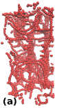
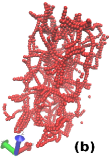
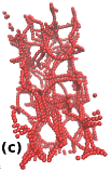
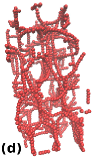
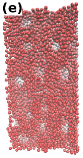
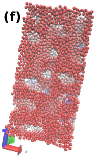
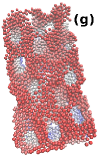
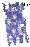
Figure 9: (colour online) The figure shows the snapshots for NPs and monomers from the NP + micellar-polymer system for the lowest value of monomer number density$\rho_{m}=0.037\sigma^{-3}$. The snapshots in the upper row show only the micellar monomers while only the nanoparticles are shown in the lower row. The snapshots from (a) to (d) [and correspondingly (e) to (h)] are for $\sigma_{4n}=2.0\sigma,2.5\sigma,3\sigma$ and $3.5\sigma$, respectively. There is a gradient in colour along one of the shorter axis of the box for the snapshots (e) to (h), to help reader differentiate the particles present near the front plane from those at the rear. All the snapshots indicate the formation of the network-like structure of aggregates of nanoparticles and micellar chains inter-penetrating each other.

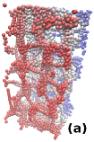
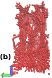
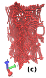
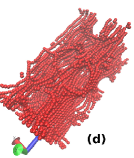
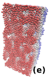
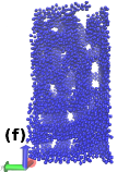
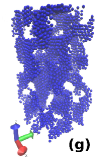
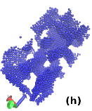
Figure 10: (Colour online) The figure shows the snapshots of NPs and monomers from the NP + micellar-polymer system for the value of monomer number density $\rho_{m}=0.074\sigma^{-3}$. The snapshots in the upper row show only the micellar monomers while, the lower row only shows the nanoparticles. Snapshots from (a) to (d) [or correspondinly (e) to (h)] are for $\sigma_{4n}=1.75\sigma,2.25\sigma,2.75\sigma$ and $3.25\sigma$, respectively. The snapshots (a) and (e) have a gradient in colour varying from red to blue along one of the shorter axis of the simulation box to help the reader diferentiate the particles at the front plane and those closer to the rear. Snapshots (e), (f), and (g) are forming network-like structures of nanoparticles, while the nanoparticle network breaks down into non-percolating clusters in the figure (h) by forming individual sheetlike nano-structures.

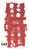
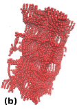
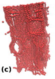
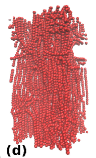
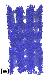
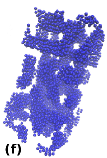
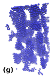
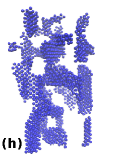
Figure 11: ( colour online). The figure shows the snapshots of NPs and monomers from the NP + micellar-polymer system for the value of number density of monomers $\rho_{m}=0.093\sigma^{-3}$. Snapshots in the upper row show only micellar monomers (red) while the snapshots in the lower row only show nanoparticles (blue). Snapshots from (a) to (d) [or correspondingly (e) to (h)] are for $\sigma_{4n}=1.75\sigma,2.25\sigma,2.5\sigma$ and $3\sigma$, respectively. With the increase in the value of $\sigma_{4n}$ from left to right, the snapshots of nanoparticles show that the network gradually breaks and form individual sheet-like clusters for a high value of $\sigma_{4n}$, as shown in the snapshot (h).

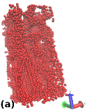
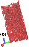
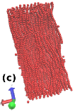
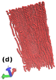
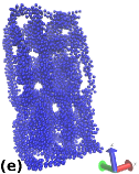
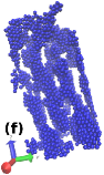
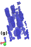
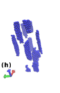
Figure 12: (colour online). Figure shows the snapshots of NPs and monomers from the NP + micellar-polymer system for monomer number density $\rho_{m}=0.126\sigma^{-3}$. The snapshots in the upper row show only micellar monomers while, only the NPs are shown in the lower row. Snapshots (a) to (d) (or (e) to (h)) correspond to $\sigma_{4n}=1.75\sigma$, $2\sigma$, $2.25\sigma$ and $2.5\sigma$, respectively. With increase in the value of $\sigma_{4n}$, the figure shows the nanoparticle networks in (e) and (f) breaking into individual rod-like nanostructures as shown in the snapshots (g) and (h).

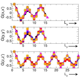
Figure 13: (colour online) The figure shows the average of the local density-density correlation function for monomers for $\sigma_{4n}=1.5\sigma$ and different values of micellar densities indicated by different symbols. The density correlations along $x,y$ and $z$-axis are shown separately from top to bottom. The different symbols are for $\rho_{m}=0.037\sigma^{-3}$ (circle-black), $0.074\sigma^{-3}$ (square-red), $0.093\sigma^{-3}$(diamond-blue), and $0.126\sigma^{-3}$ (triangle-magenta). The symbols (star-orange) indicate the correlation plots for $\rho_{m}=0.037\sigma^{-3}$ but $\sigma_{4n}=3\sigma$.

It is observed that not only the non-percolating clusters of NPs have different shapes but also the clusters which constitute the NP-networks differ in their morphologies. The snapshots in figures 9, 10(e) (& 11(e)) and 12(e) show networks of NP aggregates, network of sheet-like clusters of NPs and network of rod-like clusters of NPs, respectively. Thus the density of micelles governs the morphology of NP structures with the anisotropy of NP clusters increasing with increase in micellar density viz. clusters to sheets to rods. We also observe that as soon as the value of $\sigma_{4n}$ changes from $1.25\sigma$ (Fig.5) to $1.5\sigma$ (Fig.9(e), 10(e), 11(e), 12(e) ), the micellar chains aggregate to form clusters which joins to form a system spanning network such that the networks of micellar chains and NPs are inter-penetrating each other. These networks at $\sigma_{4n}=1.5\sigma$ seem to have the same periodicity in their structure irrespective of the micellar density.

IV.4 Polymeric chains of the matrix:
quantitative analysis of micro-structure

To confirm the above observations, we plot the density correlation function for monomers which is shown in Fig.13. It shows the density correlation function for monomers along the x, y, and z-axes of the box for $\sigma_{4n}=1.5\sigma$. The function is calculated using the expression,

$$G(x_{i},x^{\prime}_{i})=\frac{\Big{\langle}(\rho(x_{i})-\langle\rho(x^{\prime}_{i})\rangle)(\rho(x_{i})-\langle\rho(x^{\prime}_{i})\rangle)\Big{\rangle}}{\Big{\langle}(\rho(x_{i})-\langle\rho(x_{i})\rangle)^{2}\Big{\rangle}}$$ (6)

where, $\rho(x_{i})$ is the density of the monomers in cubic box of size $\sigma^{3}$ at $x_{i}$ at a particular $y-z$ plane. The angular brackets in the numerator correspond to averages taken at different $y-z$ planes as well as over different independent runs. The term $\langle\rho(x_{i})\rangle$ is the mean density of monomers in the simulation box. The term in the denominator normalizes the function from 1 to -1. The different symbols indicate the different values of micellar densities in Fig.13. All the plots for different densities overlap each other and are indistinguishable from each other. They have the same spatial period for all the densities and along different the axes. This indicates the periodic nature of the network-like structures in all three directions and this remains unaltered by the change in monomer number density. This is observed not only for the value of $\sigma_{4n}=1.5\sigma$, but also for all the values of $\sigma_{4n}$ considered for $\rho_{m}=0.037\sigma^{-3}$ (refer Fig.9).

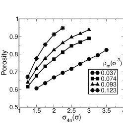
Figure 14: (colour online) The figure shows the variation in the porosity of the network of nanoparticles. Porosity is calculated by subtracting the nanoparticle volume fraction from $1$, i.e. it represents the variation in the volume fraction of the void (currently occupied by monomers, but which can be dissolved away) inside a porous network of NPs due to the change in $\sigma_{4n}$ values. The different symbols indicate the different values of micellar densities. It can be seen that the porosity of the networks increases with either increase in the value of $\sigma_{4n}$ or increase in monomer number density $\rho_{m}$, as expected.

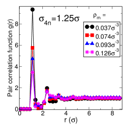
Figure 15: The figure shows the pair correlation function $g(r)$ for monomers at $\sigma_{4n}=1.25\sigma$. It shows four different plots for $\rho_{m}=0.037\sigma^{-3},0.074\sigma^{-3},0.093\sigma^{-3}$ and $0.126\sigma^{-3}$ which are indicated by different symbols in the figure. The absence of a peak around $1.75\sigma$ indicates that polymeric chains are out of the range of repulsive interaction $V_{4}$ from each other and hence depicts the dispersed state of chains, with NPs in between adjacent chains.

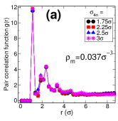
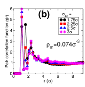
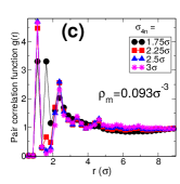
Figure 16: (colour online ). The figure shows the pair correlation function for micellar monomers for $\sigma_{4n}=1.25\sigma$ and micellar densities (a) $\rho_{m}=0.037\sigma^{-3}$, (b) $\rho_{m}=0.074\sigma^{-3}$, (c) $0.093\sigma^{-3}$ and (d) $0.126\sigma^{-3}$. Each figure shows the correlation function for four different values of $\sigma_{4n}>1.25\sigma$ as indicated in the graph. Contrary to the observations from $g(r)$ data shown in Fig.15 (for $\sigma_{4n}=1.25\sigma$), all the figures here show the appearance of peaks around $1.75\sigma$. The appearance of a peak around $1.75\sigma$ indicates that the distance between adjacent monomer chains $\approx 1.75\sigma$ (the range of $V_{4}$). Therefore, chains are forming clusters that joins to form a network-like structure as shown in Fig.9, 10, 11, 12 for $\sigma_{4n}>1.25\sigma$. With increase in the value of $\sigma_{4n}$, the height of the peak around $1.75\sigma$ decreases and finally vanishes for a higher value of $\sigma_{4n}$, except for the lowest density shown in (a) for $\rho_{m}=0.037\sigma^{-3}$. For the lowest density, the micellar chains forms networks of clusters of micellar chains for all the values of $\sigma_{4n}>1.25\sigma$ as shown in Fig.9.

For the lowest density of micelles considered here , i.e. $\rho_{m}=0.037\sigma^{-3}$, the morphological changes from network of NPs to sheets to rod-like structures is not observed for $\sigma_{4n}>1.25\sigma$. The effect of an increase in the value of $\sigma_{4n}$ is observed to decrease the number density of NPs without changing the periodicity of the networks. The plot of density correlation function for all the values of $\sigma_{4n}$ considered for $\rho_{m}=0.037\sigma^{-3}$, has the same periodicity as shown by the plots in figure. 13. To confirm this, the plots shown in figure 13 shows graphs for $\rho_{m}=0.037\sigma^{-3}$ for two different values of $\sigma_{4n}=1.5\sigma$ (circle-black symbols) and $3\sigma$ (star-orange symbols).

Furthermore, the snapshots in figure 9 show that as $\sigma_{4n}$ increases (from left to right), the pore size increases and the wall thickness (or the branch thickness of the network) is seen to be decreasing. Hence, we conclude that the thickness of the walls of the NP networks decreases as a result of an increase in $\sigma_{4n}$. This behaviour affects the porosity of the network. We define porosity as the volume fraction of the void inside the NP network. The porosity is calculated by subtracting the NP volume fraction from 1. The figure 14 shows the variation of porosity versus $\sigma_{4n}$ quantifying the observed behaviour of the porosity with increase in $\sigma_{4n}$. For a given value of $\sigma_{4n}$, an increase in micellar density decreases the available volume for NPs, thereby, increasing the porosity of the NP network. Therefore, the figure 14 also shows an increase in porosity with the increase in micellar density $\rho_{m}$ for a fixed value of $\sigma_{4n}$, as expected. The non-linear behaviour of the plot for $\rho_{m}=0.123\sigma^{-3}$ is related to the drop in the number of NPs which can get introduced in the box as one increases $\sigma_{4n}$. The nanoparticle porous structure can be obtained and used after removing by dissolving away the polymeric matrix.

In figures 9, 10, 11 and 12, we observe the clustering of NPs and micellar chains into different morphologies for values of $\sigma_{4n}\geq 1.5\sigma$ whereas, Fig.5 shows that for $\sigma_{4n}=1.25\sigma$ (the minimum possible value of $\sigma_{4n}$), we obtain a uniformly mixed state of self-assembled micellar chains and NPs. To get an insight into the spatial arrangement of micellar chains, we calculate the pair correlation function g(r) of monomers corresponding to the snapshots shown in figures 5, 9, 10, 11 and 12. The plots in Fig. 15 corresponds to correlation function for the snapshots shown in Fig.5 while the plots in figures 16(a), 16(b), 16(c) and 16(d) correspond to the snapshots shown in figures 9, 10, 11 and 12, respectively. Different symbols represents $g(r)$ for different values of $\sigma_{4n}$.

In the correlation function of monomers, a first peak is expected to occur around the value of the diameter $\sigma$ of the monomer (which is set as 1) followed by peaks at its multiples indicating the distance between bonded monomers along a chain. If there are chains that are situated at a distance $r<=1.75\sigma$ (i.e. having the repulsive interaction $V_{4}$) from other chains, then peaks around $1.75\sigma$ and its multiples are expected. We do not observe any peak around $1.75\sigma$ in Fig.15 for all the values of micellar densities. This indicates that the micellar chains in all the snapshots shown in Fig.5 (for $\sigma_{4n}=1.25\sigma$), are situated at a distance $r>1.75\sigma$. This is consistent with the observation that no two micellar chains in Fig.5 are found to exist without NPs in between. With a NP of size $1.5\sigma$ between two monomer chains, the monomer chains have no possibility to remain within the range of repulsive potential ($r\leq 1.75\sigma$). Thus, it confirms the observation that, for all the snapshots shown in Fig.5, no clustering of micellar chains is observed and a uniformly mixed state of micellar chains and NPs is formed.

In contrast to the plots in Fig.15, there appears a peak around $1.75\sigma$ in Figs.16(a), 16(b), 16(c) and 16(d). Except for the plots in Fig.16(a), it is observed that the height of this peak decreases with the increase in the value of $\sigma_{4n}$ and finally vanishes for a higher value of $\sigma_{4n}$. The appearance of a peak around $1.75\sigma$ is consistent with the observed clustering of micellar chains as shown in the snapshots in Figs.9, 10, 11 and 12 where, they form network-like structures. As the value of $\sigma_{4n}$ increases, the NP network gradually starts breaking and hence giving more space for micellar chains to be relatively further away from each other. This explains the decrease in the peak height around $1.75\sigma$ with increase in $\sigma_{4n}$. When the NP network breaks to the extent that most of the micellar chains get enough volume to be at a distance $r>1.75\sigma$, this peak disappears and a minimum is observed at that point. The value of $\sigma_{4n}$ at which this happens can be seen to be decreasing with increase in micellar density viz. $3\sigma$ and $2.25\sigma$ for $\rho_{m}=0.093\sigma^{-3}$ and $0.126\sigma^{-3}$, respectively.

However, this behaviour is not observed for $\rho_{m}=0.037\sigma^{-3}$ [refer Fig.16(a)] where for all the values of $\sigma_{4n}$ the peaks are present around $1.75\sigma$. This is because, with an increase in $\sigma_{4n}$, the network-like structure is not observed to be breaking as shown in Fig.9. Therefore, for all the values of $\sigma_{4n}$, the polymeric chains show the formation of clusters of chains that is reflected in the form of peaks around $1.75\sigma$ for all the values of $\sigma_{4n}$ in Fig.16(a).

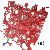
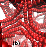
Figure 17: The representative snapshot in (a) shows only the monomer configurations from a NP + micellar-polymer system for $\sigma_{4n}=2.5\sigma$ for the lowest value of monomer number density $\rho_{m}=0.037\sigma^{-3}$ for simulations performed in a larger box size of $60\times 60\times 60\sigma^{3}$. This monomer-network is similar to the monomer-network structures obtained in a smaller box size 0f $30\times 30\times 30\sigma^{3}$ as shown in Fig.9. A magnified image of one of the network junction is shown in figure (b). Irrespective of the value of $\sigma_{4n}$, all the network structures obtained for $\rho_{m}=0.037\sigma^{-3}$ produce statistically similar monomeric network structures (with the same periodicity).

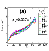
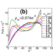
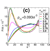
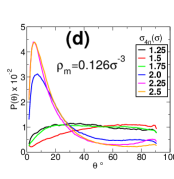
Figure 18: The figure shows the distribution of angles subtended between pairs of micellar chains at different values of monomer densities, $\rho_{m}$ = (a) $0.037\sigma^{-3}$, (b) $0.074\sigma^{-3}$, (c) $0.093\sigma{-3}$ and (d) $0.126\sigma^{-3}$, respectively. Each figure shows graphs for different values of $\sigma_{4n}$. For the lowest micellar density (a), it shows a peak at $90^{\circ}$ angle, hence confirming that many of the polymers lie to each other, as seen in snapshots of Fig.17(b). Plots in (b) and (d) show two peaks one around $10^{\circ}$ and the other around $90^{\circ}$. The peak around $10^{\circ}$ corresponds to the formation of aligned domains of micellar chains which result in sheet-like structures, while the peak around $90^{\circ}$ shows the perpendicular arrangement of these sheet-like domains. The figure (d) shows a peak for a parallel arrangement of micellar chains which in turn results in the formation of rod-shaped aggregates of nanoparticles.

For the lowest micellar density considered $\rho_{m}=0.037\sigma^{-3}$, only the network-like structures are observed for the range of values of $\sigma_{4n}$ considered here (except for the case of $\sigma_{4}=1.25\sigma$). To ensure that the network architecture observed in the snapshots in Fig.9 is not an artefact of the small box size, these structures were reproduced in a larger box size of $60\times 60\times 60\sigma^{3}$ for all values of $\sigma_{4n}$ considered for $\rho_{m}=0.037\sigma^{-3}$. A representative snapshot for $\sigma_{4n}=2.5\sigma$ and $\rho_{m}=0.037\sigma^{-3}$ is shown in fig. 17(a). The figure shows that the snapshot have statistically similar network of micellar chains as in the smaller box size shown in Fig.9. The Fig.17(b) shows a magnified image of one of the junctions of the network.

As seen in the snapshots of Figures.10(h), 11(h) and 12(g)&(h), the anisotropy of the NP clusters depends on the micellar density. Moreover, the nanoparticle clusters that form a percolating network as in Figs.9(e), 10(e), 11(e) and 12(e) also differ in their anisotropy thereby resulting in different pore shapes. Since, the structure of the nanoparticles also effects the arrangement of chains, or vice versa, the arrangement of micellar chains can be used to indirectly interpret the anisotropy of the NP structures. The distribution of angle between micellar chains $P(\theta)$ is analyzed and the plots are shown in Fig.18 for $\rho_{m}=0.037\sigma^{-3},0.074\sigma^{-3},0.093\sigma^{-3}$, and $0.126\sigma^{-3}$ from (a) to (d), respectively. It is calculated by,

$$P(\theta)=\frac{N(\theta)}{\sum_{\theta}N(\theta)}$$ (7)

where, $N(\theta)$ is the total number of pair of chains at an angle $\theta$ and the angle $\theta$ between two chains is calculated by using the largest eigenvectors of the corresponding gyration tensors of the chains as follows,

$$\theta=\cos^{-1}\frac{\vec{e_{1}}.\vec{e_{2}}}{|\vec{e_{1}}||\vec{e_{2}}|}$$ (8)

where, $\vec{e_{1}}$ and $\vec{e_{2}}$ are the largest eigenvectors of the gyration tensors of the two chains.

The distribution $P(\theta)$ is normalized for different values of $\sigma_{4n}$ by dividing it by the number of all possible combinations of the pair of chains. Each plot in Fig.18 shows the distribution of angles between micellar chains for different values of $\sigma_{4n}$ as indicated in the figures. The lowest density of micellar system considered $\rho_{m}=0.037\sigma^{-3}$ shows a high value of the distribution around 90^∘ for all values of $\sigma_{4n}$. This shows the perpendicular arrangement of micellar chains at the network junction as can be seen in the Fig.17(b). The similar correlation plots in Fig.13 and the same distribution function for angles in Fig.18(a) for $\rho_{m}=0.037\sigma^{-3}$ confirms the similarly periodic architecture of monomers networks for all $\sigma_{4n}$ as shown in Fig.9. The distribution plots for the monomer densities $\rho_{m}=0.074\sigma^{-3}$ and $0.0931\sigma^{-3}$ in figures 18(b) and (c) shows that after a particular value of $\sigma_{4n}$, there appear two peaks around $10^{\circ}$ and $90^{\circ}$ indicating a preference for a parallel and a perpendicular arrangement of micellar chains, respectively. These are the densities where NPs form sheet-like structures. The parallel arrangement indicates that the chains within an aligned micellar domain form sheet-like structures. The peak around $90^{\circ}$ in the distribution plot corresponds to the perpendicular arrangement of these sheet-like domains of aligned micellar chains. We find the formation of sheet-like domains to be unexpected and interesting and the reason for this will be explained later in the text. All the neighbouring NP sheets as shown in Figure. 10 and 11 are arranged such that their planes are perpendicular to each other. Finally for the highest micellar density considered $\rho_{m}=0.126\sigma^{-3}$, for $\sigma_{4n}\geq 2\sigma$, there appears a high peak around $10^{\circ}$. Here, the presence of peaks only around $10^{\circ}$ is indicative of the nematic ordering of micellar chains and correspondingly we observe rodlike structure of NPs. The height of the peaks at $90^{\circ}$ gradually reduces from (b) to (d) and resulting in only peaks for parallel arrangement in (d). This is indicative of the change in the anistropy of NP clusters. This can be confirmed by calculating the shape anisotropy $S_{AN}$ of NP clusters using the following formula,

$$S_{AN}=1-3\frac{\lambda_{1}\lambda_{2}+\lambda_{2}\lambda_{3}+\lambda_{1}\lambda_{3}}{(\lambda_{1}+\lambda_{2}+\lambda_{3})^{2}}$$ (9)

where, $\lambda_{1},\lambda_{2},\lambda_{3}$ are the eigen values of the gyration tensor of the NP cluster. Using the above formula, the average shape anisotropy of the nanoparticle clusters shown in snapshots of Figs.10(h), 11(h) and 12(h) is calculated to be $0.165,0.211$ and $0.414$, respectively. This shows that the shape anisotropy of the NP clusters increases with increase in micellar density and the shape of the NP clusters is varying from sheet-like to rod-like structures. This shows that the anisotropy of the NP structures increases with increase in micellar density with nanostructures varying from sheets to rodlike structures.

IV.5 The morphological changes : our understanding

The purpose of the introduction of the parameter $\sigma_{4n}$ is to control the minimum approaching distance between micelles and NPs, but it also influences the arrangement and the number of NPs in the system and hence affects the effective volume of micelles. An increase in the value of $\sigma_{4n}$ indicates an increase in the effective volume of micelles. We remind the reader that, as discussed in the beginning of the section (refer Fig.3), the effective volume of micelles also gets modified by the density of NPs present in the system. In the presence of a large number of NPs (lower value of $\sigma_{4n}$), there are relatively more contacts between monomers and NPs, which leads to a higher value of the effective volume of monomers. Moreover, the number of contacts also depend on the assembly architecture and the relative organization between NPs and micellar chains. Therefore, the effective volume of micelles not only depends on the value of $\sigma_{4n}$ but also on the NP density as well as the morphology and corresponding monomer-NP contacts. Hence, the effect of the transformation from network-like structure to non-percolating clusters can be understood in terms of change in the effective volume of micelles.

From the experimental perspective, different values of $\sigma_{4}$ would correspond to micellar chains made up of different chemical compositions such that they have different diameters of micellar chains. Here, it is kept constant ($\sigma_{4}=1.75\sigma$). Now, with a given value of $\sigma_{4}$ and micellar density, it is the parameter $\sigma_{4n}$ that effectively determines the space available for the incoming NPs inside the simulation box. Experimentally, in the micelle-NP mixture, the effective repulsion between micellar chains of a particular composition (with a particular value of $\sigma_{4}$) and NPs can be tuned in to change the value of $\sigma_{4n}$ and thereby the effective volume available to NPs. That, in turn, will determine the morphology of NP mesostructures formed in the presence of a background micellar matrix.

A characteristic quantity that changes with the density of monomers is the average length of monomer chains. The average chain length of WLMs increases with increase in the value of monomer density. In presence of a large number of NPs (in case of system spanning network of NPs), monomers are more packed. This is also seen from the behaviour of $g(r)$ in Fig.16) and can be compared to the systems with a lower number of NPs which result in non-percolating clusters. Therefore, the effect of the change of NP morphology from network to non-percolating clusters is expected to be seen in the value of average chain length of micelles. We first discuss the behaviour of the average length of micellar chains with a change in $\sigma_{4n}$, because, that will help us quantitatively better appreciate the behaviour of the effective volume fraction of micelles.

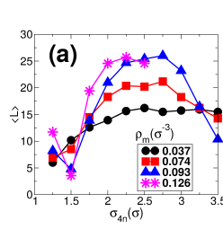
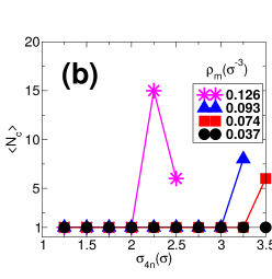
Figure 19: (colour online) Figure (a) shows the variation in the average length $\langle L\rangle$ of micellar chains with $\sigma_{4n}$ where, L is the number of monomers in a particular chain. The figure (b) shows the plot for number of nanoclusters $\langle N_{c}\rangle$ in the system. The quantity $\langle L\rangle$ shows a decrease in its value at a higher value of $\sigma_{4n}$ where nanoparticle network breaks into non-percolating clusters. The quantity $<N_{c}>$ shows a jump from its value of $1$ to a larger value when, the nanoparticle network breaks into non-percolating clusters.The nanoparticles aggregates with $<N_{c}>=1$ spans the length of the simulation box as seen in the snapshots and also confirmed by calculating the largest eigen value of the gyration tensor for these aggregates.

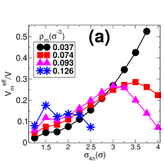
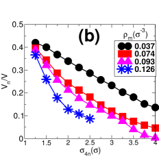
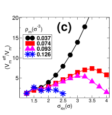
Figure 20: (colour line) The figure shows the behaviour of (a) effective monomer volume fraction (${V_{m}}^{eff}/V$), (b) nanoparticle volume fraction ($V_{n}/V$) and (c) the ratio of effective monomer volume to the monomer volume (${V_{m}}^{eff}/{V_{m}}$), with change in the value of $\sigma_{4n}$, where $V_{m}=\rho_{m}4/3\pi(\sigma/2)^{3}V$. Each figure shows graphs for four different values of number density of monomers i.e. $\rho_{m}=0.037\sigma^{-3},0.074\sigma^{-3},0.093\sigma^{-3}$ and $0.125\sigma^{-3}$ as indicated by the symbols. With an increase in the value of $\sigma_{4n}$, the nanoparticle volume fraction in (b) decreases while the effective monomeric volume fraction in (a) increases. At a higher value of $\sigma_{4n}$, the monomeric volume fraction shows a decrease in its value indicating a change of nanoparticle structure from network to non-percolating clusters. In figure (c), the graph represents the variation of the ratio of the effective monomer volume fraction to the monomer volume fraction. In other words, it represents the extent of the effect of the repulsive interactions on effective monomer volume fraction. A high value of ${V_{m}}^{eff}/{V_{m}}$ indicates that the presence of a large number of interacting pairs having repulsive interactions $V_{4}$ and $V_{4n}$, which have a cutoff distances $\sigma_{4}$ and $\sigma_{4n}$, respectively. The graph in (c) shows high values for intermediate values of $\sigma_{4n}$, where the system shows the formation of a network-like structure of nanoparticles. However, for very low values or high values of $\sigma_{4n}$, the ratio $V_{m}/{V_{m}}^{eff}$ shows low values ($\sim 0.1$ for $\rho_{m}=0.126\sigma^{-4}$). This shows that the constituent particles in the system are away from each other, i.e., at a distance greater than the cutoff distances of the repulsive interactions $V_{4}$ and $V_{4n}$, for very low or higher values of $\sigma_{4n}$.

The behaviour of average micellar chain length is shown in Fig.19(a). Different symbols indicate different micellar number densities. The average length at $\sigma_{4n}=1.25\sigma$ increases with increase in the number density of monomers. This is also consistent with the snapshots shown in Fig.5. In that figure, we observe longer chains for higher values of monomer number densities. An increase in the value of $\sigma_{4n}$ from $1.25\sigma$ to $1.5\sigma$, reverses this behaviour. This is due to the fact that, at $\sigma_{4n}=1.5\sigma$, the micellar chains undergo a change in their arrangement from dispersed to network-like structure with clusters of micellar chains. This transition is such that the network-like structure of NPs has the same period for all micellar densities (refer Fig.13 and the corresponding snapshots in Fig.9, 10(a), 11(a) and 12(a)). At $\sigma_{4n}$ $=1.5\sigma$, with the same periodicity of NP networks (refer Fig.13), micellar chains with a high $\rho_{m}$ are more ”crushed” (having smaller chains) compared to the systems with lower density. Therefore, denser micellar systems have lower average length of micellar chains for this particular value of $\sigma_{4n}$. This can also be realised by comparing the snapshots shown in Fig.9(a), 10(a), 11(a) and 12(a). With further increase in the value of $\sigma_{4n}$, the NP networks start breaking. Due to the presence of higher number of monomer-nanoparticle contacts in the systems with higher monomer densities, the effect of the increase in the value of $\sigma_{4n}$ is also higher. Therefore, for the same increase in the value of $\sigma_{4n}$ beyond $1.5\sigma$, the decrease in the number of nanoparticles is more for a higher value of $\rho_{m}$. Hence, the nanoparticle network is “more broken” for higher $\rho_{m}$. Hence, the average length reverses its behaviour at $1.75\sigma$, and the average length again increases with $\rho_{m}$ as was seen for the $\sigma_{4n}=1.25\sigma$ system.

As explained earlier, the effective polymeric chain volume depends on the combination of the value of $\sigma_{4n}$, the NP number density and more importantly, the number of contacts with NP and monomers. Therefore, at a higher value of $\sigma_{4n}$ ($>2.5\sigma$ when the introduction of NPs inside the system becomes relatively difficult), the effective micellar volume decreases and hence a decrease in the average length of micellar chains can be seen. This decrease in the average length shows the extent of the breaking of NP network, and the breaking of network-like structures to non-percolating clusters of NPs is recorded once the average length of chains start to decrease. This occurs at $\sigma_{4n}=2.25\sigma,3.25\sigma$ and $3.5\sigma$ for the values of micellar densities $\rho_{m}=0.126\sigma^{-3},0.093\sigma^{-3}$ and $0.074\sigma^{-3}$, respectively. Thus, the behaviour of the average length of micelles clearly indicates the existence of two points of structural changes. The first one is for the change from dispersed state to clustering of micellar chains (from $\sigma_{4n}=1.25\sigma$ to $\sigma_{4n}=1.5\sigma$) and the other is for the breaking of NP network into non-percolating clusters at some higher value of $\sigma_{4n}$ depending on micellar density.

Since the change in average length indirectly indicates a change in effective volume of micelles, a decrease in the effective volume of micelles is expected around the point of transformation. To confirm these observations, the behaviour of the volume fractions of the constituents and the average energies of NPs and monomers are examined, and the plots are shown in Figs.20 and 21, respectively.

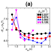
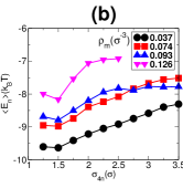
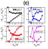
Figure 21: The Figure shows graphs for variation in the average potential energy (PE) of (a) monomers, (b) nanoparticles and for different values of monomer densities. Plot (c) shows the monomer and NP PEs in the same plot, but each subfigure shows data for a particular value of $\rho_{m}$. With an increase in the value of $\sigma_{4n}$, the nanoparticle energy decreases while the energy of micelles increases. At a higher value of $\sigma_{4n}$, the monomer volume fraction shows a decrease in its value marking the change from network-like structure to non-percolating clusters of nanoparticles. In (c), the lines showing variation in monomer PE (filled symbols) and PE of nanoparticles (empty symbols) intersect at some intermediate value of $\sigma_{4n}$. The change from network to non-percolating clusters of the nanoparticle takes place at a value of $\sigma_{4n}$ higher than the $\sigma_{4n}$-value at which the intersection occurs. The points of intersections of the energies of monomers and nanoparticles for different values of monomer densities are indicated by the vertical lines which get shifted to lower values of $\sigma_{4n}$ with the increase in micellar densities. Therefore, with an increase in the micellar densities the point of change of nanoparticle morphology from network to non-percolating clusters also gets shifted to a lower value of $\sigma_{4n}$.

The Fig.20 shows (a) the plot of the effective monomer volume fraction ${V_{m}}^{eff}/V$ (b) NP volume fraction $V_{n}/V$ and (c) the ratio of effective volume fraction of monomers to monomers volume fraction ${V_{m}}^{eff}/V_{m}$. Change in the value of $\sigma_{4n}$ from $1.25\sigma$ to $1.5\sigma$ corresponds to the formation of clusters of micellar chains from a dispersed state as discussed before. These clusters of micellar chains join to form a system spanning network-like structure. With further increase in $\sigma_{4n}$, the effective volume fraction of monomers increases at first but then starts to decrease after a certain value of $\sigma_{4n}$ ($>2.5\sigma$) for the highest three number densities. The decrease in the value of the effective volume fraction of monomers corresponds to the transition from the network-like structure of nanoparticles to non-percolating clusters. This happens at $\sigma_{4n}=2.25\sigma$ for $\rho_{m}=0.126\sigma^{-3}$, $\sigma_{4n}=3.25\sigma$ for $\rho_{m}=0.093\sigma^{-3}$ and at $\sigma_{4n}=3.5\sigma$ for $\rho_{m}=0.074\sigma^{-3}$. This change in nanoparticle structure is not observed for the lowest density of micelles for the values of $\sigma_{4n}$ considered here. Hence, ${V_{m}}^{eff}/V_{m}$ keeps on increasing for $\rho_{m}=0.037\sigma^{-3}$. In Fig.20(b), the nanoparticle volume fraction decreases with increase in $\sigma_{4n}$ as introducing nanoparticles in the system becomes increasingly difficult with increasing $\sigma_{4n}$.

The ratio of the effective volume fraction of monomers to their actual volume fraction [refer Fig.20(c)] shows the extent of the effect of $\sigma_{4n}$ on the effective volume fraction of micelles. Its behaviour is exactly similar to the behaviour of the effective volume of monomers. The behaviour of the ratio ${V_{m}}^{eff}/V_{m}$ indicates the role of $\sigma_{4n}$ and micellar density in the arrangement of constituent particles and hence the morphology of the system. A high value of ${V_{m}}^{eff}/V_{m}$ is obtained when there exists a clustering of micellar chains as a consequence of an increase in $\sigma_{4n}$. When $(V_{m}^{eff}/V_{m})\approx 1$, it shows a dispersed state of micellar chains.

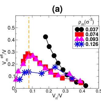
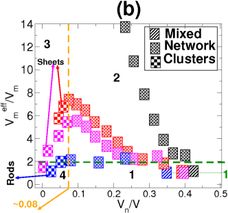
Figure 22: (a) The figure shows the effective volume fraction ${V_{m}}^{eff}/V$ of equilibrium polymers (micelles) versus the nanoparticle volume fraction $V_{n}/V$. The vertical broken line (orange) separates the values of $V_{n}/V$ which correspond to formation of network morphology of NPs and micelles (right of the vertical line) from the $V_{n}/V$ values which correspond to the non-percolating clusters of NPs (left of vertical line). The exceptions to network morphology are the points with highest nanoparticle volume fraction for each $rho_{m}$. These correspond to the mixed phase of NPs and micellar chains. (b) The figure shows the replot of the figure shown in (a) with the variable shown in Y-axis replaced by the ratio of ${V_{m}}^{V_{m}}$ and the symbols indicating the morphology of the system. These two lines divide the graph into four different regions marked as 1, 2, 3 and 4. The points in region-1 are for $\sigma_{4n}=1.25\sigma$ which form a dispersed state (no clustering) of micellar chains (all joined by a (thin-green) horizontal line intersecting the Y-axis at $\approx 1$). Region-2 shows the systems with network-like structures of both nanoparticles and micellar chains. Regions-3 belongs to the systems forming non-percolating clusters of nanoparticles in between the clusters of micellar chains. Finally, the region-4 depicts the systems with non-percolating clusters of nanoparticles in the background matrix of dispersed micellar chains.

The Fig.21 shows the graphs of average energy per particle of (a) monomers $\langle E_{m}\rangle$ and (b) NPs $\langle E_{n}\rangle$. The plot in (c) shows the average energy per particle for both monomers (filled symbols) and NPs (empty symbols), with data for different values of densities shown in separate graphs. For the change in $\sigma_{4n}$ from $1.25\sigma$ to $1.5\sigma$, the $\langle E_{m}\rangle$ shows an increase in its value for $\rho_{m}=0.126\sigma^{-3}$ and $\rho_{m}=0.093\sigma^{-3}$ while, it decreases for $\rho_{m}=0.074\sigma^{-3}$ and $\rho_{m}=0.037\sigma^{-3}$. This change corresponds to the transition of polymeric chains from dispersed state to the network of its clusters. We can consider that these networks are formed in between the network of nanoparticle aggregates. This is because the volume fraction of nanoparticles is higher than the effective volume fraction of monomers. The network of monomer chains show same periodicity of the structure for all $\rho_{m}$ (refer Fig.13) at $\sigma_{4n}=1.5\sigma$. Therefore, the monomers with number densities $\rho_{m}=0.126\sigma^{-3}$ and $\rho_{m}=0.093\sigma^{-3}$ are ”crushed” in between nanoparticle clusters forming smaller chains compared to the systems with number densities $\rho_{m}=0.037\sigma^{-3}$ and $\rho_{m}=0.074\sigma^{-3}$ (refer Fig.19).

The existence of smaller chains in the box increases the values of both $V_{2}$ and $V_{4}$ for $\rho_{m}=0.126\sigma^{-3}$ and $\rho_{m}=0.093\sigma^{-3}$. Hence, the energy of monomers $\langle E_{m}\rangle$ shows an increase in its value for $\rho_{m}=0.126\sigma^{-3}$ and $\rho_{m}=0.093\sigma^{-3}$ but decreases for $\rho_{m}=0.037\sigma^{-3}$ and $\rho_{m}=0.074\sigma^{-3}$, for the same change in value of $\sigma_{4n}$ from $1.25\sigma$ to $1.5\sigma$. For the same change in $\sigma_{4n}$ (from $1.25\sigma$ to $1.5\sigma$), the energy of NPs $\langle E_{n}\rangle$ show a decrease in their value. This decrease in nanoparticle energy is a result of an increase in the packing of nanoparticles due to increase in $\sigma_{4n}$.

With further increase in $\sigma_{4n}$, $\langle E_{m}\rangle$ decreases while $\langle E_{n}\rangle$ shows an increase. This decrease in the $\langle E_{m}\rangle$ is due to the increase in the effective volume fraction of monomers whcih results in an increased chain length. However, $\langle E_{m}\rangle$ again shows an increase after $\sigma_{4n}=2\sigma$, $\sigma_{4n}=3\sigma$ and $\sigma_{4n}=3.25\sigma$ for $\rho_{m}=0.126\sigma^{-3}$, $\rho_{m}=0.093\sigma^{-3}$ and $\rho_{m}=0.074\sigma^{-3}$, respectively. This increase in the value of $\langle E_{m}\rangle$ corresponds to the breaking of nanoparticle network into non-percolating clusters that results in the decrease in micellar chain length (refer Figs.19 and 20(a)). Thus the dependence of average monomer energy on $\rho_{m}$ changes for the change in $\sigma_{4n}$ from $1.25\sigma$ to $1.5\sigma$, this is a consequence of the change from dispersed state of chains of monomers to network-like structure.

Moreover, the transition from nanoparticle network to non-percolating clusters is also indicated by an increase in $\langle E_{m}\rangle$ for higher values of $\sigma_{4n}>1.5\sigma$. In Fig.21(c) shows the variation in $E_{m}$ and $E_{n}$ with $\sigma_{4n}$ on the same plot for each value of $\rho_{m}$, the points of intersection of both the energies are shown by vertical lines (dashed). As the NP network gradually breaks with increase in $\sigma_{4n}$, the NP energy decreases and energy of monomers increases. At a value of $\sigma_{4n}$, just higher than the point of intersection of these two energy plots, the nanoparticle network breaks into individual clusters. With the decrease in micellar density $\rho_{m}$, the point of intersection of the two energies gets shifted to higher values of $\sigma_{4n}$. Therefore, the value of $\sigma_{4n}$ at which the NP network breaks into non-percolating clusters also gets shifted to higher values with the decrease in micellar density.

All these observations can be well explained in a plot of effective micellar volume fraction versus NP volume fraction which is shown in Fig.22(a). Different monomer number densities are represented by different symbols. The orange coloured dashed vertical line divides the parameter region where NP network structures are observed from the region of parameters where NPs form non-percolating clusters. All the points to the left of this line show the systems with non-percolating clusters of NPs, while all the points to the right show the percolating network-like structures of both NPs and polymeric chains. The rightmost point for each case of micellar density (the maximum value of NP volume fraction for each $\rho_{m}$) belongs to the system which has polymeric chains dispersed in between NPs. In this plot, the regions having the points showing uniformly dispersed and network-like structures of micellar chains are not well separated and they overlap. If we replot this graph with the variable along the Y-axis replaced by ${V_{m}}^{eff}/V_{m}$, then the regions with the dispersed and the network of clusters of micellar chains can also be captured and both the morphological transformations can be clearly marked on the graph. This is shown in Fig.22(b).

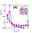
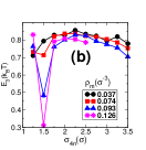
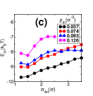
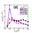
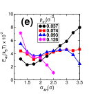
Figure 23: The figure shows the variations of the potential energies due to (a) $V_{2},(b)V_{3},(c)V_{2n},(d)V_{4}$ and (e) $V_{4n}$ with the excluded volume parameter $\sigma_{4n}$. The potentials are explained in the modeling section. All the points are represented along with the error bars for $10$ independent runs. The error bars are too low to be visible for all the plots.

In Fig.22(b), the ratio ${V_{m}}^{eff}/V_{m}$ shows the extent of the effect of change in $\sigma_{4n}$ on the effective volume of micelles (refer Fig.20(c)). The different morphologies of the system are indicated by the different symbols. For any symbol, the different colours correspond to the different micellar densities. At $\sigma_{4n}=1.25\sigma$ and for all the values of $\rho_{m}$, the value of the ratio ${V_{m}}^{eff}/V_{m}$ remains $\approx 1$. All such points are joined by a horizontal line (thin-broken-green) intersecting the Y-axis at $\approx 1$. An increase in the value of $\sigma_{4n}$ from $1.25\sigma$ to $1.5\sigma$ leads to the onset of formation of clusters of micellar chains. All such points with a network-like structure of polymeric chains are indicated by the corresponding symbol spanning over a large parameter space in the graph. All the points that show a network-like structure of clusters of micellar chains occurs above a value of ${V_{m}}^{eff}/V_{m}\approx 2$ that is shown by a dashed horizontal line (green). Therefore, this line approximately marks the change from a uniformly dispersed state to a network-like structure of micellar chains. With further increase in $\sigma_{4n}$, the NP volume fraction decreases and effective monomer volume fraction increases. At a even higher value of $\sigma_{4n}$ (depending on $\rho_{m}$), the NP networks break to form non-percolating clusters. This is marked by an decrease in the value of the effective volume of micelles and all such points are shown by the corresponding symbol for non-percolating clusters of NPs. Depending on the number density of monomers, the morphology of these non-percolating clusters changes from sheets to rodlike structures (with increasing $\rho_{m}$). For all the values of $\rho_{m}$, the change from network-like morphology to non-percolating clusters of NPs is observed to occur at a value of NP volume fraction $\approx 0.08$. This is marked by a dashed vertical line (orange).

The combination of the vertical line (orange-broken) and the horizontal line (green-broken) divides the space into four different regions which are marked as 1, 2, 3 and 4. Each region defines the structural morphology of the system as follows;
Region 1: Uniformly mixed state of micellar chains and nanoparticles with micellar chains dispersed in between nanoparticles.
Region 2: Both the polymeric chains and the nanoparticles form network-like structures which interpenetrate each other.
Region 3: Individual clusters of nanoparticles in between the clusters of micellar chains.
Region 4: In this region all the points show the value of $\frac{{V_{m}}^{eff}}{V_{m}}\approx 1$, therefore, the monomer chains are in a dispersed state. However, the nanoparticles form non-percolating clusters. Therefore, in this region, non-percolating clusters of nanoparticles are present in the background of dispersed chains of micelles.

All the observations discussed in this paper for the NP-micellar system can be verified by examining the behaviour of the potential energies involved in the system. The plots of these potential energies $E_{2},E_{3},E_{2n},E_{4},E_{4n}$ are shown in Figs.23(a), (b), (c), (d) and (e) due to the potentials $V_{2},V_{3},V_{2n},V_{4}$ and $V_{4n}$, respectively. All the potential energy values are averaged over 10 independent runs with $(15-20)\times 10^{5}$ iterations for each run and are plotted with an error bar. The error bars are too small to be visible. Moreover, these potential energies are normalized by dividing them with the number of all combinations of the particles that are interacting with the concerned potential. A higher value of $E_{2}$ indicates a higher average length of the chains and vice versa. The behaviour of $E_{2}$ in Fig.23(a) shows an increase in its value for a change of $\sigma_{4n}=1.25\sigma$ to $1.5\sigma$ for $\rho_{m}=0.126\sigma^{-3}$ and $\rho_{m}=0.093\sigma^{-3}$ indicating scission of chains. Apart from these two points $E_{2}$ decreases with increase in $\sigma_{4n}$ for all monomer densities indicating the increase in chain lengths. However, with further increase in $\sigma_{4n}$, it shows a decrease in its value (except $\rho_{m}=0.037\sigma^{-3}$). This happens at $\sigma_{4n}=2.25\sigma$ for $\rho_{m}=0.126\sigma^{-3}$ and at $\sigma_{4n}=3.25\sigma$ for $\rho_{m}=0.093\sigma^{-3}$ and $0.074\sigma^{-3}$. Thus, it confirms the behaviour of the average length of chains shown in Fig.19.

Figure 23(b) shows the behaviour of $E_{3}$ with $\sigma_{4n}$ for different values of $\rho_{m}$. Longer chains will give rise to a large number of bonded triplets along a chain resulting in a higher value of $E_{3}$ while, smaller chains will result in a lower value of $E_{3}$. Therefore, the decrease in the value of $E_{3}$ for change of $\sigma_{4n}=1.25\sigma$ to $1.5\sigma$ for $\rho_{m}=0.126\sigma^{-3}$ and $\rho_{m}=0.093\sigma^{-3}$ is indicative of the formation of smaller chains at $1.5\sigma$. Moreover, with further increase in the value of $\sigma_{4n}$, $E_{3}$ shows relatively higher values indicating the presence of longer chains. The interaction potential energies between NPs $E_{2n}$, shown in Fig.23(c), also shows a decrease at $1.5\sigma$ indicating an increase in the packing of nanoparticles in spite of the decrease in its number density. It then shows an increase in its value at a higher value of $\sigma_{4n}$ due to a decrease in its number density.

The potential energies $E_{4}$ in Fig.23(d) which shows the repulsive interaction between micellar chains shows an increase in its value when the micellar chains transforms to a network-like structure at $\sigma_{4n}=1.5\sigma$ from a dispersed state at $\sigma_{4n}=1.25\sigma$. The quantity $E_{4}$ then decreases indicating that the average distance between micellar chains increases (chains get out of the range of the potential $E_{4}$) as $\sigma_{4n}$ increases. The repulsive interaction energy between NPs and micellar chains $E_{4n}$ shown in Fig.23(e) also shows the two points of morphological transformations, first a decrease in $E_{4n}$ at $\sigma_{4n}=1.5\sigma$ indicating the change in the structure of micellar chains from dispersed to clusters that join to form network-like structure. The decrease in $E_{4n}$ is due to the re-organization of micellar chains to form clusters that reduces the number of monomer-NPs contacts. Then, it increases (or remains constant for $\rho_{m}=0.126\sigma^{-3}$), but again show a decrease in its value when the morphology of NPs changes from a network-like structure to non-percolating clusters. This decrease is due to the low density of NPs present in the system at high $\sigma_{4n}$. The values of the repulsive potential energies $E_{4}$ and $V_{4n}$ are of the order of $10^{-2}k_{B}T$, thereby, indicating that the rearrangement of the system architecture with the increase in $\sigma_{4n}$ is to avoid the repulsive interactions within the system.

Thus, the plots of $E_{4}$ and $E_{4n}$ with very low values (of the order of $10^{-2}k_{B}T$) points to the emergence of different kind of self-assembled structures as a result of the system trying to decrease the interfacial or repulsive interactions. The repulsive interaction potential between NPs and micellar chains $V_{4n}$ will form a phase separated state at higher densities in order to reduce the repulsion between them. But the presence of the steep repulsive interaction potential within the micellar chains ($V_{4}$) themselves evokes a competition between the two potentials $V_{4}$ and $V_{4n}$. Micellar chains aligned parallely with the average distance between chains $r<\sigma_{4}$, lead to a higher value of the potential energy due to $V_{4}$. Therefore, reducing the value of $V_{4}$ as well as $V_{4n}$ not only requires a reduction of the interface area between micelles and NPs but also encourages micellar chains to arrange such that they are out of the range of the repulsive interaction $V_{4}$ acting between themselves. For a system with low monomer density (Fig.9), the perpendicular arrangement between micellar chains which meet at the junctions of the network (refer Fig.17(b) and fig.18) is a consequence of the requirement to reduce the repulsive interaction between them. By remaining at an angle of $90^{\circ}$, the possibility of the chains of monomers coming in contact with each other is very low. With an increased density of micelles (Fig.10 and 11), the average length of the micellar chains also increases. Therefore, for higher monomer density if the same structures as shown in figure 9 is maintained, it will lead to an increased width of the clusters of micellar chains in the network resulting in a high repulsive energy due to $V_{4}$. Hence, the micellar chains arrange in an aligned fashion forming thin sheet-like domains and relatively away from each other in order to reduce values of $V_{4}$. The steep increase of the potential $V_{4}$ with $r_{4}$ discourages those Monte Carlo steps which bring the monomers from adjacent chains just below $\sigma_{4}$, and thus the values of $E_{4}$ remains much lower than $k_{B}T$. Micellar chains which form sheet like domains have relatively lower number of neighbouring chains compared to chains in a hexagonally packed arrangement. Moreover, the arrangement of these sheetlike planes at an angle perpendicular to neighbouring domains (as noted in Figure. 18(b) and (c)) also seems to be the part of the strategy to lower the repulsive potential between micellar chains by reducing the possibility of contact between the domains. At even higher number densities of micelles, the chains become very long and formation of a sheet-like structure would lead to an increase in the interfacial area between micellar sheets and NPs. This in turn will result in an increase potential energy due to $V_{4n}$. Therefore, in this case, the NPs prefer to nematically arrange themselves with the polymeric chains maintaining a distance $r>1.75\sigma$ from each other to be out of the range of the repulsive potential $V_{4}$.

V Discussion and Conclusion:

In this paper, we examine in detail the behavior of mixtures attractive nanoparticle (NPs) and equilibrium polymers (EPs), examples of which are worm-like micellar systems, with the variation of number of monomer number density and the excluded volume parameter (EVP) between micellar chains and nanoparticles. The density of monomers which self-assemble to form equilibrium polymers affect the self organization of aggregates of NPs, which in turn affect the affect the organization and length of the self-assembled polymeric chains. One obtains a number of interesting equilibrium or kinetically arrested configurations of NP morphologies, starting from a mixed phase of NPs and EPs, when the size of NPs are relatively small compared the width of micellar chains. For higher values of the EVP, the morphology of the NP aggregates varies from porous percolating connected network of NPs, where the thickness of the pores can be suitably controlled by the EVP and number density of monomers, to disconnected aggregates of NPs with varying shape anisotropy values. The NPs aggregate between clusters of semi-flexible polymeric chains, hence instead of nucleating to spherically symmetric aggregates they develop into anisotropic rod like aggregates whih grow parallel to the allignment of backgroun semi-flexible micellar matrix. We establish that the anisotropy of the NP clusters is governed by the density of the equilibrium polymeric matrix. Furthermore, the steep repulsive potential between neighboring micellar chains, and its contribution relative to repulsive potential between chains and NPs, can lead to the formation of planar sheet like arrangement of micellar chains due to self-avoidance, which in turn lead to planar sheets of NP-aggregates. Apriori, this was was an unexpected result for us. This and the other morphologies obtained are examples of the production of nanostructures via synergistic interactions of the equilibrium polymeric matrix and the NPs. The value of the volume fraction of NPs for the transformation from network-like morphology to non-percolating clusters of NPs is approximately identified as $\approx 0.08$. We summarize the different kinetically arrested morphologies obtained in a (non-equilibrium) phase diagram with the effective volume fraction of EPs and the volume fraction of NPs on the two axes. There have been experimental studies Helgeson et al. (2010) which explore the fundamental aspects of Wormlike micelle and NP interactions, where they see “double network” of micelles and NPs. But there the underlying interactions are expected to be different, with chains getting attached to NPs to to form a network of micelles. We have purely repulsive interaction between chains and NPs.

Understanding the underlying physical mechanism and energetics of the different morphologies obtained due to synergistic interactions between self-assembling polymers and attractive NPs is expected to help the experimental scientist fine tune the relevant parameters to control the yield of different porous nano-structures with required surface area and porosity. The micelles can be dissovled away once the NPs aggregate and self-organize to the suitable morphology. This might have significant relevance, for example, in the design of batteries materials and super-capacitors, where one needs to balance between large surface area (to increase charge storage) as well as large pores to enable quick dynamics of ions during the charging and discharging process, which affects power density. On the other hand, the NPs could also be possibly dissolved away after the self assembled polymers are made into gels by addition of suitable additives to enable the experimentalist to obtain polymeric sponges as has been demonstrated using ice-templating techniques Biswas et al. (2016); Chatterjee et al. (2017). We expect the EP-NP morphologies to be kinetically arrested phase separating states, except when the value of $\sigma_{4n}=1.25\sigma$ when we get a thermodynamically stable mixed state. We use grand-canonical Monte Carlo scheme to introduce (and remove) NPs at randomly chosen positions in the box, this might seem difficult to realize experimentally in a relatively dense polymeric matrix. However, one could possibly have background solution in which the monomers self assemble to form equilibrium polymers, and then appopriately chemical reagents could be added so initiate nucleation of nano-particles out of the solution which would then aggregate and self-organize into the suitable morphologies depending on the synegistic interactions with the background polymeric matrix.

VI Acknowledgement

We acknowledge the helpful discussion with Dr.Arijit Bhattacharyya, Dr.Guruswamy Kumaraswamy and Dr. Deepak Dhar. We thank the computational facility provided National Param Super Computing (NPSF) CDAC, India for use of Yuva cluster, the compute cluster in IISER-Pune, funded by DST, India by Project No. SR/NM/NS-42/2009. We acknowledge funding and the use of a cluster bought using DST-SERB grant no. EMR/2015/000018 to A. Chatterji. AC acknowledges funding support by DST Nanomission, India under the Thematic Unit Program (grant no.: SR/NM/TP-13/2016).

References

- Miyashita (2004) T. Miyashita, Nettowaku Porima 25, 34 (2004).
- Black et al. (2006) C. Black, K. Guarini, G. Breyta, M. Colburn, R. Ruiz, R. Sandstrom, E. Sikorski, and Y. Zhang, Journal of Vacuum Science & Technology B: Microelectronics and Nanometer Structures Processing, Measurement, and Phenomena 24, 3188 (2006).
- Orski et al. (2011) S. V. Orski, K. H. Fries, S. K. Sontag, and J. Locklin, Journal of Materials Chemistry 21, 14135 (2011).
- Shenhar et al. (2005) R. Shenhar, T. B. Norsten, and V. M. Rotello, Advanced Materials 17, 657 (2005).
- Zhang et al. (2004) M. Zhang, M. Drechsler, and A. H. Müller, Chemistry of materials 16, 537 (2004).
- Jayaraman and Schweizer (2009) A. Jayaraman and K. S. Schweizer, Macromolecules 42, 8423 (2009).
- Thompson et al. (2002) R. B. Thompson, V. V. Ginzburg, M. W. Matsen, and A. C. Balazs, Macromolecules 35, 1060 (2002).
- Sun et al. (2002) S. Sun, S. Anders, H. F. Hamann, J.-U. Thiele, J. Baglin, T. Thomson, E. E. Fullerton, C. Murray, and B. D. Terris, Journal of the American Chemical Society 124, 2884 (2002).
- Haryono and Binder (2006) A. Haryono and W. H. Binder, Small 2, 600 (2006).
- Lin et al. (2005) Y. Lin, A. Böker, J. He, K. Sill, H. Xiang, C. Abetz, X. Li, J. Wang, T. Emrick, S. Long, et al., Nature 434, 55 (2005).
- Rozenberg and Tenne (2008) B. Rozenberg and R. Tenne, Progress in Polymer Science 33, 40 (2008).
- Arraudeau et al. (1989) J. Arraudeau, J. Patraud, and L. Gall, “Composition based on cationic polymers, anionic polymers and waxes for use in cosmetics,” (1989), uS Patent 4,871,536.
- Tatum and Wright (1988) J. P. Tatum and R. C. Wright, “Organoclay materials,” (1988), uS Patent 4,752,342.
- Gadberry et al. (1997) J. F. Gadberry, M. Hoey, and C. E. Powell, “Organoclay compositions,” (1997), uS Patent 5,663,111.
- Patel et al. (2006) H. A. Patel, R. S. Somani, H. C. Bajaj, and R. V. Jasra, Bulletin of Materials Science 29, 133 (2006).
- Lochhead (2008) R. Y. Lochhead, HAPPI 3, 08 (2008).
- Corcorran et al. (2004) S. Corcorran, R. Y. Lochhead, and T. McKay, Cosmetics and Toiletries 119, 47 (2004).
- Laufer and Dikstein (1996) A. Laufer and S. Dikstein, Cosmetics and toiletries 111, 91 (1996).
- Lochhead (2007) R. Y. Lochhead, “The role of polymers in cosmetics: Recent trends,” in Cosmetic Nanotechnology (ACS Publications, 2007) Chap. 1, pp. 3–56, https://pubs.acs.org/doi/pdf/10.1021/bk-2007-0961.ch001 .
- Katz (2007) L. M. Katz, “Nanotechnology and applications in cosmetics: General overview,” in Cosmetic Nanotechnology (ACS Publications, 2007) Chap. 11, pp. 193–200, https://pubs.acs.org/doi/pdf/10.1021/bk-2007-0961.ch011 .
- Miller (2006) G. Miller, Nanomaterials, sunscreens and cosmetics: small ingredients big risks (Friends of the Earth, 2006).
- Raj et al. (2012) S. Raj, S. Jose, U. Sumod, and M. Sabitha, Journal of Pharmacy & Bioallied Sciences 4, 186 (2012).
- Sorrentino et al. (2007) A. Sorrentino, G. Gorrasi, and V. Vittoria, Trends in Food Science & Technology 18, 84 (2007).
- De Azeredo (2009) H. M. De Azeredo, Food Research International 42, 1240 (2009).
- Rhim et al. (2013) J.-W. Rhim, H.-M. Park, and C.-S. Ha, Progress in Polymer Science 38, 1629 (2013).
- Arora and Padua (2010) A. Arora and G. Padua, Journal of Food Science 75 (2010).
- Ray et al. (2006) S. Ray, S. Y. Quek, A. Easteal, and X. D. Chen, International Journal of Food Engineering 2 (2006), retrieved 31 Mar. 2018, from doi:10.2202/1556-3758.1149.
- Sozer and Kokini (2009) N. Sozer and J. L. Kokini, Trends in Biotechnology 27, 82 (2009).
- Sambarkar et al. (2012) P. Sambarkar, S. Patwekar, and B. Dudhgaonkar, International Journal of Pharmacy and Pharmaceutical Sciences 4, 60 (2012).
- Ray and Bousmina (2006) S. S. Ray and M. Bousmina, Polymer nanocomposites and their applications (American Scientific, 2006).
- Mouriño (2016) V. Mouriño, in Nanocomposites for Musculoskeletal Tissue Regeneration, edited by H. Liu (Woodhead Publishing, Oxford, 2016) pp. 175 – 186.
- Dwivedi et al. (2013) P. Dwivedi, S. S. Narvi, and R. P. Tewari, Journal of Applied Biomaterials & Functional Materials 11, 129 (2013).
- Ingrosso et al. (2010) C. Ingrosso, A. Panniello, R. Comparelli, M. L. Curri, and M. Striccoli, Materials 3, 1316 (2010).
- Segala and Pereira (2012) K. Segala and A. S. Pereira, in New Polymers for Special Applications, edited by A. D. S. Gomes (InTech, Rijeka, 2012) Chap. 07.
- Striccoli et al. (2009) M. Striccoli, M. Curri, and R. Comparelli, in Toward Functional Nanomaterials (Springer, 2009) pp. 173–192.
- Mazumdar et al. (2015) P. Mazumdar, S. Rattan, and M. Mukherjee, RSC Advances 5, 69573 (2015).
- Carotenuto and Nicolais (2004) G. Carotenuto and L. Nicolais, Polymer International 53, 2009 (2004), https://onlinelibrary.wiley.com/doi/pdf/10.1002/pi.1616 .
- Qi (2017) H. Qi, Novel Functional Materials Based on Cellulose (Springer, 2017).
- Bloemer and Scalora (1998) M. J. Bloemer and M. Scalora, Applied Physics Letters 72, 1676 (1998).
- Jakšić et al. (2004) Z. Jakšić, M. Maksimović, and M. Sarajlić, Journal of Optics A: Pure and Applied Optics 7, 51 (2004).
- Scalora et al. (1998) M. Scalora, M. Bloemer, A. Pethel, J. Dowling, C. Bowden, and A. Manka, Journal of Applied Physics 83, 2377 (1998).
- Kedawat et al. (2014) G. Kedawat, B. K. Gupta, P. Kumar, J. Dwivedi, A. Kumar, N. K. Agrawal, S. S. Kumar, and Y. K. Vijay, ACS Applied Materials & Interfaces 6, 8407 (2014).
- Gence et al. (2010) L. Gence, V. Callegari, S. Melinte, S. Demoustier-Champagne, Y. Long, A. Dinescu, and J. Duvail, in Nanowires Science and Technology (InTech, 2010).
- Park et al. (2004a) S. Park, S.-W. Chung, and C. A. Mirkin, Journal of the American Chemical Society 126, 11772 (2004a).
- Das and Prusty (2012) T. K. Das and S. Prusty, Polymer-Plastics Technology and Engineering 51, 1487 (2012).
- Turberfield (2003) A. Turberfield, Physics World 16, 43 (2003).
- Park et al. (2004b) S. H. Park, H. Yan, J. H. Reif, T. H. LaBean, and G. Finkelstein, Nanotechnology 15, S525 (2004b).
- Alam et al. (2013) M. Alam, A. Siddiqui, M. Husain, et al., Express Polymer Letters 7, 723 (2013).
- Dijkstra et al. (1999) M. Dijkstra, J. M. Brader, and R. Evans, Journal of Physics: Condensed Matter 11, 10079 (1999).
- Ilett et al. (1995) S. M. Ilett, A. Orrock, W. Poon, and P. Pusey, Physical Review E 51, 1344 (1995).
- Lekkerkerker et al. (1992) H. Lekkerkerker, W.-K. Poon, P. Pusey, A. Stroobants, and P. . Warren, EPL (Europhysics Letters) 20, 559 (1992).
- Poon (2002) W. Poon, Journal of Physics: Condensed Matter 14, R859 (2002).
- Asakura and Oosawa (1954) S. Asakura and F. Oosawa, The Journal of Chemical Physics 22, 1255 (1954).
- Aarts et al. (2002) D. Aarts, R. Tuinier, and H. Lekkerkerker, Journal of Physics: Condensed Matter 14, 7551 (2002).
- Bolhuis et al. (2002) P. Bolhuis, A. Louis, and J. Hansen, Physical review letters 89, 128302 (2002).
- Gast et al. (1983) A. Gast, C. Hall, and W. Russel, Journal of Colloid and Interface Science 96, 251 (1983).
- De Hek and Vrij (1981) H. De Hek and A. Vrij, Journal of Colloid and Interface Science 84, 409 (1981).
- Fleer et al. (2007) G. J. Fleer, A. M. Skvortsov, and R. Tuinier, Macromolecular Theory and Simulations 16, 531 (2007).
- Poon et al. (1997) W. Poon, A. Pirie, M. Haw, and P. Pusey, Physica A: Statistical Mechanics and its Applications 235, 110 (1997).
- Zhang et al. (2013) I. Zhang, C. P. Royall, M. A. Faers, and P. Bartlett, Soft Matter 9, 2076 (2013).
- Starrs et al. (2002) L. Starrs, W. Poon, D. Hibberd, and M. Robins, Journal of Physics: Condensed Matter 14, 2485 (2002).
- Joshi (2014) Y. M. Joshi, Annual Review of Chemical and Biomolecular Engineering 5, 181 (2014).
- Kresge et al. (1992) C. Kresge, M. Leonowicz, W. J. Roth, J. Vartuli, and J. Beck, Nature 359, 710 (1992).
- Seul and Andelman (1995) M. Seul and D. Andelman, Science 267, 476 (1995).
- Tang et al. (2006) Z. Tang, Z. Zhang, Y. Wang, S. C. Glotzer, and N. A. Kotov, Science 314, 274 (2006).
- Van Workum and Douglas (2006) K. Van Workum and J. F. Douglas, Physical Review E 73, 031502 (2006).
- Bedrov et al. (2005) D. Bedrov, G. D. Smith, and L. Li, Langmuir 21, 5251 (2005).
- Shay et al. (2001) J. S. Shay, S. R. Raghavan, and S. A. Khan, Journal of Rheology 45, 913 (2001).
- Fejer and Wales (2007) S. N. Fejer and D. J. Wales, Physical Review Letters 99, 086106 (2007).
- Glotzer and Solomon (2007) S. C. Glotzer and M. J. Solomon, Nature Materials 6, 557 (2007).
- Lee et al. (2004) J. Y. Lee, A. C. Balazs, R. B. Thompson, and R. M. Hill, Macromolecules 37, 3536 (2004).
- Xu et al. (2017) N. Xu, Q. Zhang, H. Yang, Y. Xia, and Y. Jiang, Scientific Reports 7, 43970 (2017).
- Sun and Yang (2008) H. Sun and B. Yang, Science in China Series E: Technological Sciences 51, 1886 (2008).
- Guo et al. (2014) Q. Guo, R. Ghadiri, T. Weigel, A. Aumann, E. L. Gurevich, C. Esen, O. Medenbach, W. Cheng, B. Chichkov, and A. Ostendorf, Polymers 6, 2037 (2014).
- Luo et al. (2006) Y. Luo, Z. Zheng, C. Xu, Z. Xie, and Z. Zhang, Materials Science and Engineering: A 432, 69 (2006).
- Abyaneh et al. (2016) M. K. Abyaneh, P. Parisse, and L. Casalis, Beilstein journal of nanotechnology 7, 809 (2016).
- Cao and Wang (2004) G. Cao and Y. Wang, Nanostructures and nanomaterials: synthesis, properties, and applications (World Scientific, 2004).
- Wang (2013) Z. L. Wang, Nanowires and nanobelts: materials, properties and devices. Volume 1: Metal and Semiconductor Nanowires (Springer Science & Business Media, 2013).
- Umar et al. (2008) A. Umar, S. H. Kim, and Y.-B. Hahn, Current Applied Physics 8, 793 (2008).
- Lao et al. (2006) C. S. Lao, P. X. Gao, R. S. Yang, Y. Zhang, Y. Dai, and Z. L. Wang, Chemical physics letters 417, 358 (2006).
- Singh et al. (2010) S. Singh, E. S. Kumar, M. Kottaisamy, and M. R. Rao, in AIP Conference Proceedings, Vol. 1276 (AIP, 2010) pp. 37–42.
- Pandey et al. (2016) R. K. Pandey, U. Rana, C. Chakraborty, S. Moriyama, and M. Higuchi, ACS Applied Materials & Interfaces 8, 13526 (2016).
- Vyborna et al. (2017) Y. Vyborna, S. Altunbas, M. Vybornyi, and R. Häner, Chemical Communications 53, 12128 (2017).
- Xu (2013) Q. Xu, Nanoporous materials: synthesis and applications (CRC Press, 2013).
- Ying et al. (1999) J. Y. Ying, C. P. Mehnert, and M. S. Wong, Angewandte Chemie International Edition 38, 56 (1999).
- Sharma et al. (2009) K. P. Sharma, G. Kumaraswamy, I. Ly, and O. Mondain-Monval, The Journal of Physical Chemistry B 113, 3423 (2009).
- Ramos et al. (2000) L. Ramos, P. Fabre, F. Nallet, and C.-Y. Lu, The European Physical Journal E: Soft Matter and Biological Physics 1, 285 (2000).
- Sallen et al. (1995) L. Sallen, P. Oswald, J. Géminard, and J. Malthête, Journal de Physique II 5, 937 (1995).
- Berret (2006) J.-F. Berret, in Molecular gels (Springer, 2006) pp. 667–720.
- Turner and Cates (1990) M. Turner and M. Cates, Journal de Physique 51, 307 (1990).
- Cates (1990) M. Cates, Journal of Physical Chemistry 94, 371 (1990).
- Li et al. (2010) S. Li, M. Meng Lin, M. S. Toprak, D. K. Kim, and M. Muhammed, Nano reviews 1, 5214 (2010).
- Ambrosetti (2010) G. Ambrosetti, On the insulator-conductor transition in polymer nanocomposites (EPFL, 2010).
- Chatterji and Pandit (2001) A. Chatterji and R. Pandit, Europhysics Letters 54, 213 (2001).
- Chatterji and Pandit (2003) A. Chatterji and R. Pandit, Journal of Statistical Physics 110, 1219 (2003).
- Mubeena and Chatterji (2015) S. Mubeena and A. Chatterji, Physical Review E 91, 032602 (2015).
- Helgeson et al. (2010) M. E. Helgeson, T. Hodgdon, E. W. Kaler, N. J. Wagner*, M. Vethamuthu, and K. P. Ananthapadmanabhan, Langmuir 26, 8049 (2010).
- Biswas et al. (2016) B. Biswas, C. K. Choudhury, and G. Kumaraswamy, Faraday Discussions 186, 61 (2016).
- Chatterjee et al. (2017) S. Chatterjee, P. Doshi, Kumaraswamy, and G., Soft Matter 13, 5731 (2017).