Edge-Preserving Piecewise Linear Image Smoothing Using Piecewise Constant Filters
Abstract
Most image smoothing filters in the literature assume a piecewise constant model of smoothed output images. However, the piecewise constant model assumption can cause artifacts such as gradient reversals in applications such as image detail enhancement, HDR tone mapping, etc. In these applications, a piecewise linear model assumption is more preferred. In this paper, we propose a simple yet very effective framework to smooth images of piecewise linear model assumption using classical filters with the piecewise constant model assumption. Our method is capable of handling with gradient reversal artifacts caused by the piecewise constant model assumption. In addition, our method can further help accelerated methods, which need to quantize image intensity values into different bins, to achieve similar results that need a large number of bins using a much smaller number of bins. This can greatly reduce the computational cost. We apply our method to various classical filters with the piecewise constant model assumption. Experimental results of several applications show the effectiveness of the proposed method.
1 Introduction
Edge-preserving image smoothing is a fundamental processing procedure in several low level computer vision applications, please refer to the applications in [3, 4, 5, 6, 7, 9, 13] for examples. For most smoothing filters in the literature, they assume the smoothed output images are piecewise constant. This can be simply modeled as:
| (1) |
where represents the expected output pixel value at position , is the expected constant value of pixel values inside the th region in the image which is denoted as . Note that can have different definitions for different methods. For example, it can be a regular patch (e.g., square patch) in bilateral filter [17] while it can be an irregular image region separated by edges in gradient norm smoothing [18].
Filters of above assumption include bilateral filter [17], joint bilateral filter [13], adaptive manifold filter [7], domain transform filter [6], median filter or weighted median filter [20], etc. The above mentioned filters are usually denoted as local methods in the literature [8]. There are also global methods that are based on the piecewise constant model assumption in Eq. (1) such as gradient norm smoothing [18] and total variation smoothing [14]. In this paper, we denote the filters based on the piecewise constant model assumption in Eq. (1) as piecewise constant filters. The corresponding filtering process is denoted as piecewise constant smoothing.
Although the piecewise constant model can meet the need of most applications, it may not work well for some special applications such as image detail enhancement, HDR tone mapping, etc. For these applications, a piecewise linear model is more preferred. Piecewise constant filters, especially those local methods mentioned above, can cause artifacts such as gradient reversals [8] in these applications. Although most global methods are capable of handling with this kind of artifacts such as the weighted least squares framework in [5], there are also global methods that can cause such artifacts, for example, the gradient norm smoothing [18] that will be shown in this paper.
In contrast to the piecewise constant model assumption, the recently proposed guided image filter [8] and its variants [2, 11, 16] are based on a piecewise linear model which can be formulated as:
| (2) |
where is the expected output pixel value at position , is the corresponding pixel value of guidance image at position . and remain constant inside the window . The model in Eq. (2) is piecewise linear with respect to the guidance image . These methods show no gradient reversal artifacts in several applications where the bilateral filter [17] shows clear gradient reversal artifacts. We denote the guided filter [8] and its variants [2, 11, 16] as piecewise linear filters and denote their corresponding smoothing procedures as piecewise linear smoothing.
In this paper, we also assume a piecewise linear model of the output image. However, our model is a spatially piecewise linear one which is different from the model of guided image filter [8] in Eq. (2). In addition, our method focuses on how to perform piecewise linear smoothing using classical piecewise constant filters. The contributions of this paper are as follows:
-
1.
We show a simple yet very effective framework to perform piecewise linear smoothing built upon several classical piecewise constant filters including bilateral filter [17], adaptive manifold filter [7], normalized convolution of domain transform filter [6], weighted median filter [20] and gradient norm smoothing [18]. Comprehensive experimental results of image detail enhancement, HDR tone mapping and flash/no-flash image filtering show that our method can perfectly eliminate gradient reversal artifacts caused by the original piecewise constant filters.
-
2.
Some accelerated methods such as the weighted median filter in [20] need to quantize image intensity values into different bins. In most cases, a large number of bins are usually needed to avoid quantization artifacts. In contrast, we show that our method based on the weighted median filter [20] can properly eliminate quantization artifacts with a much smaller number of bins, which greatly reduces the computational cost.
2 The Method
2.1 Piecewise Linear Smoothing Using Piecewise Constant Filters
Different from the piecewise linear model in Eq. (2), we formulate images with a piecewise linear model as:
| (3) |
where and are some linear coefficients that are assumed to remain constant inside . is defined the same as that in Eq. (1). In this way, Eq. (3) is a spatially piecewise linear model. It is thus different from the model in Eq. (2) which is linear with respect to the guidance image. In fact, Eq. (3) is known as linear polynomial regression which is also adopted in [1] to eliminate the staircasing effect in image denoising. However, as we will show in the next paragraphs in this section, our method is different from the method in [1]. In their method, the linear coefficients (i.e., and ) are explicitly calculated. In contrast, our method focuses on how to perform piecewise linear smoothing using piecewise constant filters where both and do not need to be explicitly calculated.
Unlike the model in Eq. (2) which is used for the explicit formulation of the filter [8], the model in Eq. (3) is a general and abstract model which is not used for explicit formulations of filters in this paper. However, when we take the derivative of with respect to , then we have:
| (4) |
Note that is by definition the gradient of the image at . Now it is simple to have the following conclusion: for images of the spatially piecewise linear model in Eq. (3), their gradients are piecewise constant. By comparing Eq. (4) with Eq. (1), it is clear that they are very similar. The only difference is that what on the left side of Eq. (1) are image intensities while they are image gradients on the left side of Eq. (4). Similarly, we can smooth image gradients with classical piecewise constant filters mentioned in Sec. 1. However, the difference is that this procedure assumes the corresponding images of the smoothed output gradients are spatially piecewise linear as modeled in Eq. (3).
However, the problem of this procedure is that we cannot simply reconstruct an image only from its smoothed gradients. Note that we also have the input image at the same time. The problem of using the input image and its filtered gradients to reconstruct the filtered image has already been studied by Xu et al. [19]. For an input image , its -axes and -axes gradients are denoted as and respectively. By denoting the smoothing process of piecewise constant filters as , then the piecewise linear output image can be reconstructed by minimizing the following energy proposed by Xu et al. [19]:
| (5) |
Note that although we adopt the reconstruction procedure proposed by Xu et al. [19], our work is completely different from theirs. Their method focuses on implementing classical filters with deep neural networks. Their method still performs piecewise constant smoothing if their implementation is based on a piecewise constant filter. In contrast, our method focuses on how to perform piecewise linear smoothing using piecewise constant filters.
Based on the statement above, we can perform piecewise linear smoothing using piecewise constant filters in the following two steps: (1) Smoothing the -axes and -axes gradients and of the input image with . can be any piecewise constant filter such as bilateral filter [17] and gradient norm smoothing [18]. The smoothed output gradients are denoted as and . (2) Using Eq. (5) to reconstruct the output image from , and with a proper value of . Then the reconstructed is spatially piecewise linear as modeled in Eq. (3).
2.2 Piecewise Constant Smoothing vs Piecewise Linear Smoothing
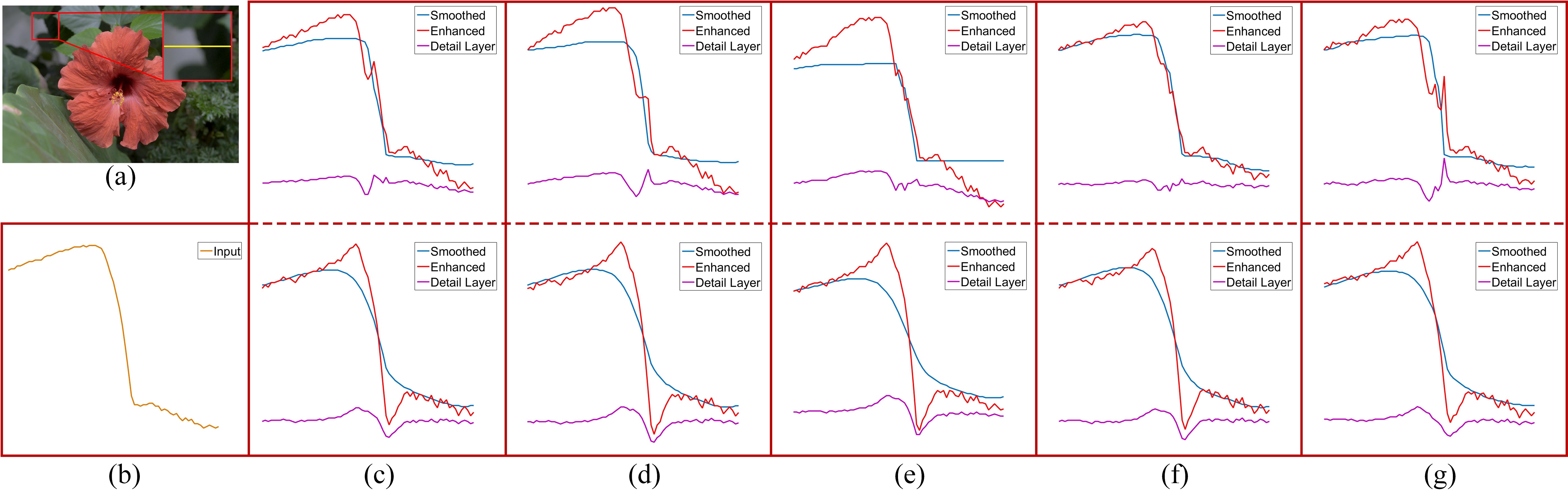
Firstly, we compare the smoothing quality of classical piecewise constant smoothing and the proposed piecewise linear smoothing applied to these piecewise constant filters. As stated in Sec. 1, classical piecewise constant filters are more suitable for piecewise constant images regions. When the image region is more likely to be piecewise linear, piecewise constant filters may cause artifacts. We show a 1D illustration in Fig. 2(b) where a piecewise linear model is more suitable for this 1D signal. We show the smoothed signals, their corresponding detail layers and enhanced signals by classical piecewise constant filters in the first row of Fig. 2(c)(g). Clearly, the detail layers cannot correctly reflect the details in the original signal. As a result, clear artifacts (known as gradient reversals) exist in the enhanced signals. In contrast, all the detail layers obtained by the proposed piecewise linear smoothing in the second row of Fig. 2(c)(g) can properly reflect the details in the original signal. Thus, no gradient reversal artifacts exist in their enhanced signals.
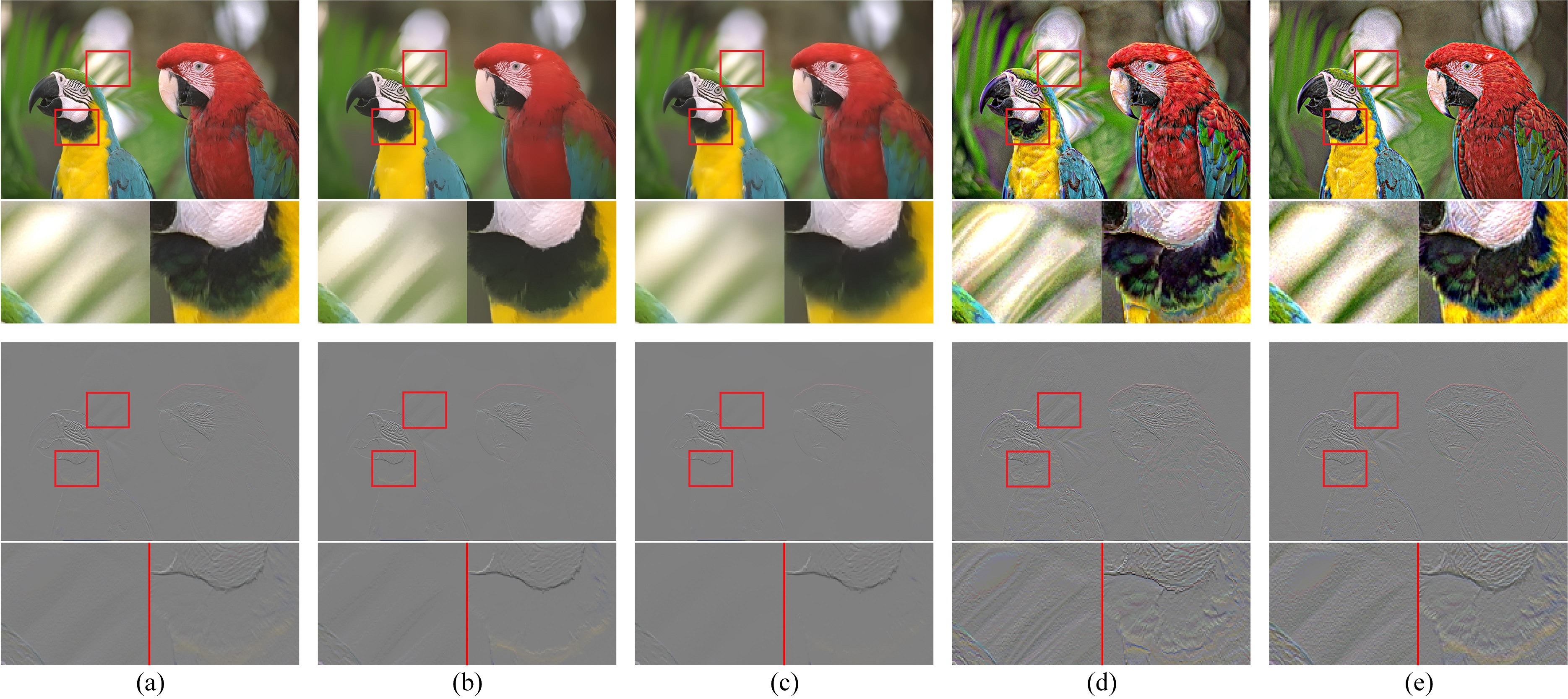
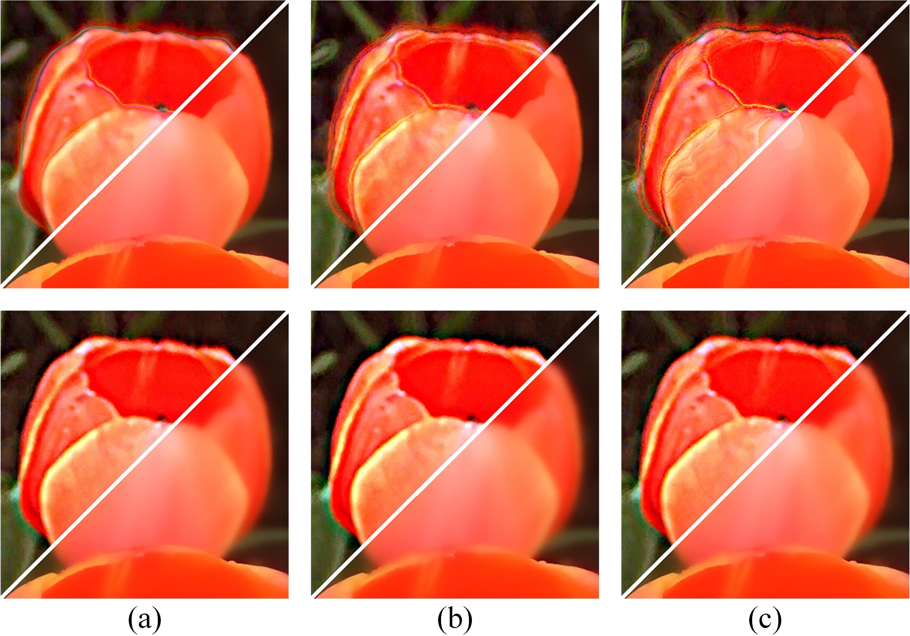
To further compare the behavior of piecewise constant smoothing and piecewise linear smoothing for strong edges and weak edges, we show a more clear visual comparison in the gradient domain in Fig. 3. As shown in highlighted regions, both two kinds of smoothing can properly preserve strong gradients which means strong edges are properly preserved. For weak edges of small gradients which should be smoothed out, piecewise linear smoothing can properly smooth out these small gradients as shown in the second row of Fig. 3(c). However, these gradients are not properly smoothed by piecewise constant smoothing or even improperly sharpened as shown in the second row of Fig. 3(b). As a result, clear gradient reversal artifacts exist in its enhanced image and the corresponding gradients in Fig. 3(d) while no gradient reversal artifacts exist in the enhanced results of piecewise linear smoothing in Fig. 3(e). This gradient domain comparison shows that the proposed piecewise linear smoothing is more accurate than classical piecewise constant smoothing in term of “edge-preserving smoothing” which means to smooth weak edges but preserve strong edges.
Secondly, we compare the computational cost of classical piecewise constant smoothing and their corresponding piecewise linear smoothing. There are two steps in the proposed piecewise linear smoothing. The first step needs to smooth both -axes gradients and -axes gradients with classical piecewise constant filters. The computational cost of this step is twice of that of the corresponding classical piecewise constant smoothing. The second step requires to solve a linear system of which the computational cost only depends on the image size. We use preconditioned conjugate gradient (PCG) to speed up the sparse linear system with the incomplete Cholesky factorization preconditioner [15] which is the same as that in [19]. This step costs 0.3 seconds for a one-megapixel RGB image. In summary, the computational cost of the proposed piecewise linear smoothing is 0.3 seconds plus twice of that of the corresponding piecewise constant smoothing for a one-megapixel RGB image.
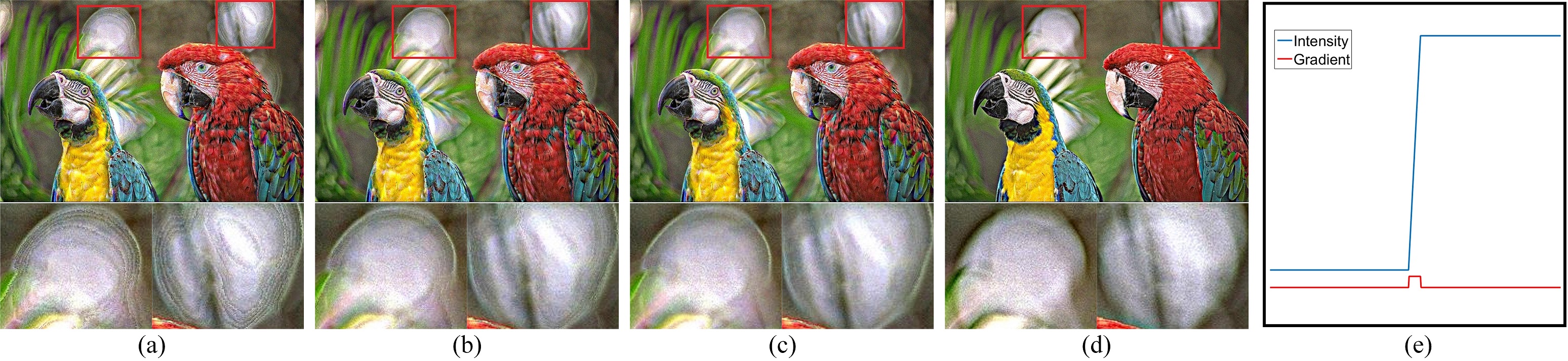
However, for accelerated methods such as the weighted median filter in [20] which need to quantize image intensity values into different bins, we find our method can further reduce the computational cost which is in contrast to the analysis above. For most cases, the accelerated piecewise constant filters usually need a large number of bins to avoid quantization artifacts while the proposed piecewise linear smoothing only needs a much smaller number of bins to achieve similar results. Fig. 4(a) shows image detail enhancement with the weighted median filter in [20] using quantization bins where clear quantization artifacts exist. When adopting bins, weak quantization artifacts still exist as shown in highlighted regions in Fig. 4(b). These quantization artifacts disappear when adopting bins as shown in Fig. 4(c). In contrast, the result of the proposed piecewise linear smoothing in Fig. 4(d) is obtained with only quantization bins and no quantization artifacts exist. This greatly reduces the computational cost from 19.32 seconds to 2.56 seconds. The reason for this phenomena is clear. The classical piecewise constant smoothing is performed in the intensity domain where intensity values could be very large as illustrated in Fig. 4(e). In contrast, the first step of the proposed piecewise linear smoothing is performed in the gradient domain. Very large intensity values can always have gradients of very small amplitude as illustrated in Fig. 4(e). Thus, to achieve a similar quantization error precision, gradient domain only needs much fewer quantization bins than intensity domain does.
2.3 Further Discussions
Compared with classical piecewise constant smoothing, there is one additional parameter of the proposed piecewise linear smoothing which is in Eq. (5). A natural question is how to choose the value of for different filters and applications. In the work of Xu et al. [18], the value of is decided as the one that has highest PSNR between the output and the “ground truth” which is the output of classical piecewise constant filters. However, there is no “ground truth” for the proposed piecewise linear smoothing. Thus, the value of is empirically decided for different filters and applications. Fig. 5 shows example results obtained with different values of . A clear observation is that increasing the value of can increase the smoothing strength. In our experiments, we empirically set for all the filters in image detail enhancement and for all the filters in HDR tone mapping. For flash/no-flash filtering, we empirically set to better smooth the heavy noise in no-flash images. Note that other parameter settings may also achieve promising results.
As stated above, can affect the final smoothing results which means that Eq. (5) can also affect the final smoothing results. A rigorous question is that whether the improvement of the proposed piecewise linear smoothing over the classical piecewise constant smoothing results from the image reconstruction step of Eq. (5). To answer this question, we perform another experiment: using the gradients of images smoothed by classical piecewise constant filters to reconstruct the final smoothed images. Note that this procedure is to perform piecewise constant smoothing. We show comparison with the proposed piecewise linear smoothing in Fig. 6. Clearly, using gradients of images smoothed by classical piecewise constant filters for image reconstruction still has the problem of gradient reversal artifacts. Thus, we can conclude that the improvement of the proposed piecewise linear smoothing results from the spatially piecewise linear model in Eq. (3).
3 Applications and Experimental Results
We apply our method to several classical piecewise constant filters to perform piecewise linear smoothing. These filters include bilateral filter [17], adaptive manifold filter [7], normalized convolution of domain transform filter [6], gradient norm smoothing [18] and weighted median filter [20]. For bilateral filter, we adopt its fast implementation in [12]111Source code can be downloaded here: http://people.csail.mit.edu/jiawen/software/bilateralFilter.m. Implementation of the other filters can be downloaded from their project websites. We perform experiments in image detail enhancement, HDR tone mapping and flash/no-flash image filtering to validate the effectiveness of the proposed method. In all applications, input images, including the gradients in the proposed piecewise linear smoothing, are firstly normalized into range before smoothing and then normalized back to their original range after smoothing. For the problem of parameter setting, we adopt the ones used in previous papers. For example, the parameters of bilateral filter [17] for all the applications in this paper are the same as those adopted in the paper of guide image filter [8]. For adaptive manifold [7], domain transform filter [6] and weighted median filter, we set their parameters analogous to those of bilateral filter for fair comparisons. The parameter of gradient norm smoothing [18] is set the same as that in its original paper. For more experimental results, please refer to our supplementary materials.
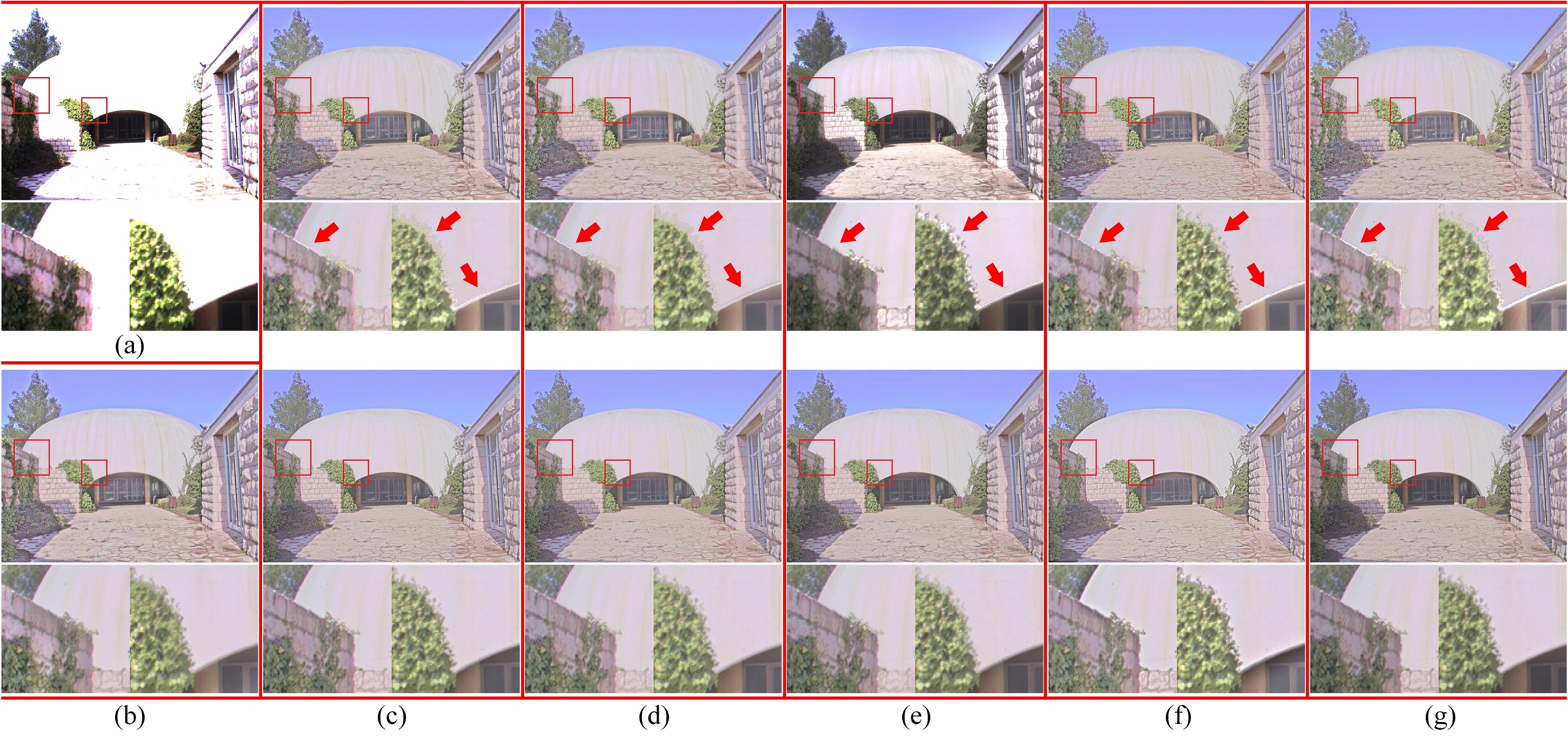
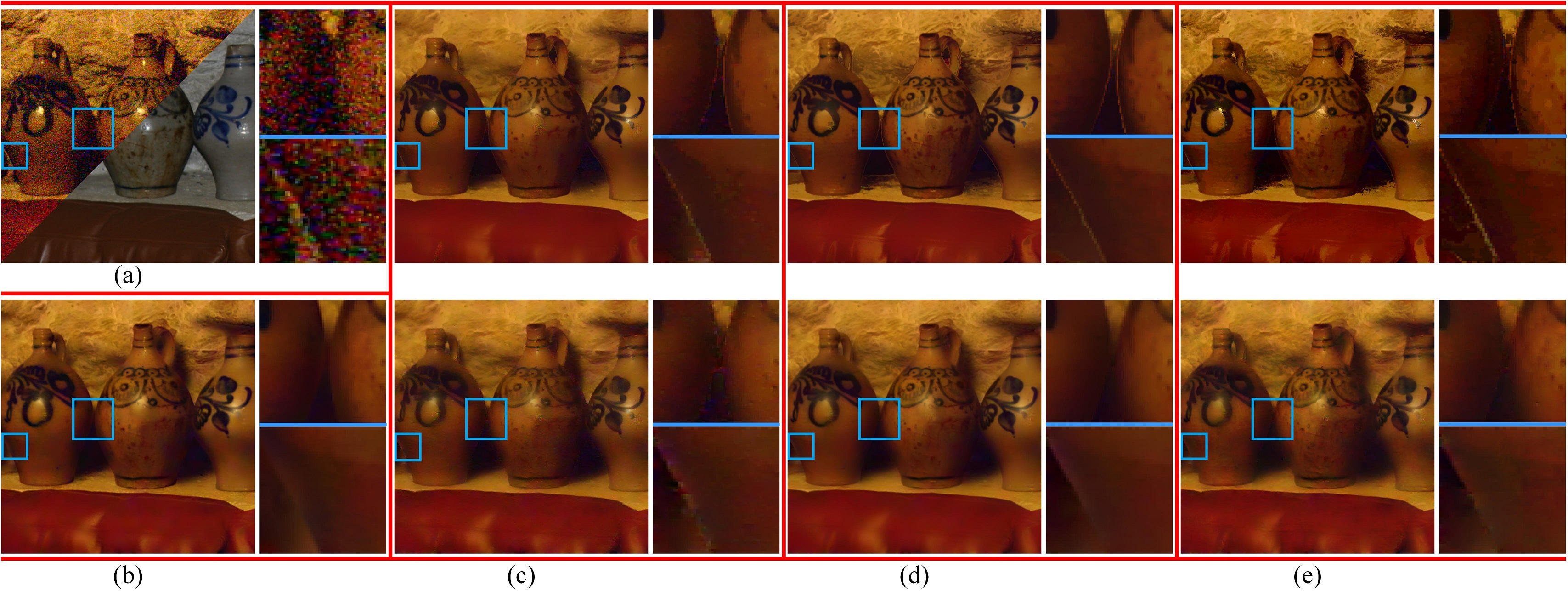
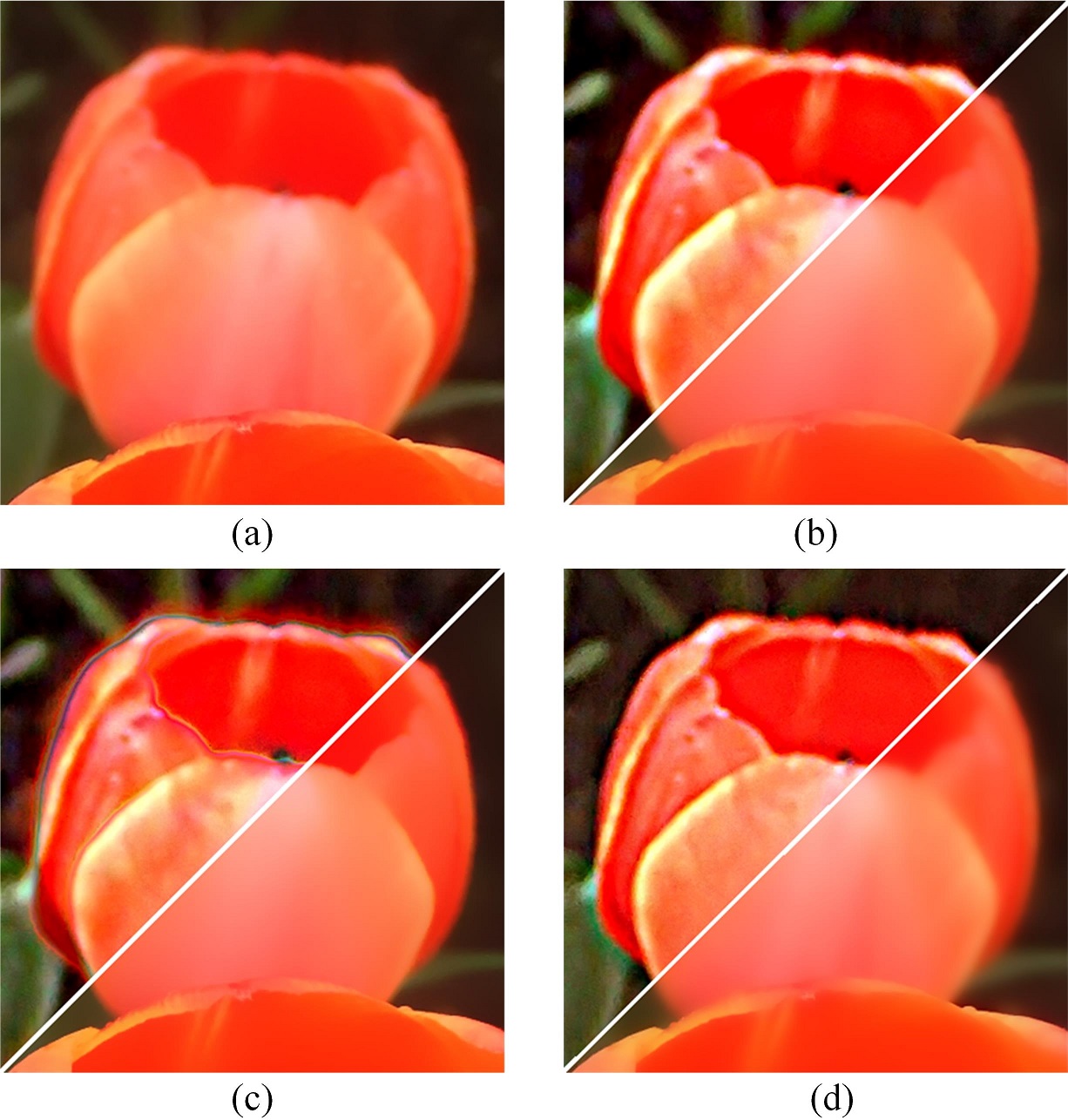
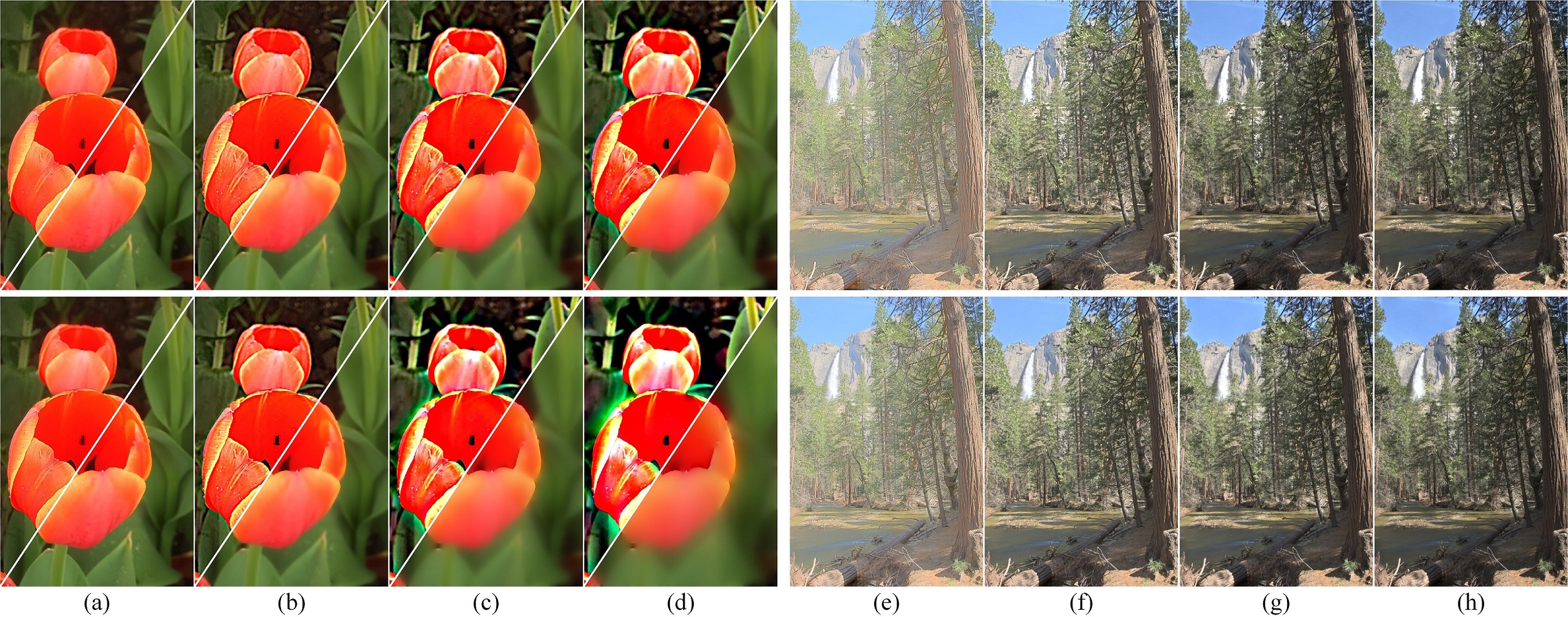
Image detail enhancement is a fundamental application of image smoothing. By subtracting the smoothed image from the original input image, we obtain the detail layer which contains the high-frequency details of the original input image. Then the detail layer is magnified and added back to the original input image to get the detail enhanced image. If edges in the smoothed image are sharper than those in the original input image, then these edges will be boosted in a reverse direction which causes the gradient reversal artifacts [5, 8]. Gradient reversal artifacts are quite common in local piecewise constant filters such as the ones mentioned in the first paragraph of this section. There are also global methods such as the gradient norm smoothing [18] that also have such problems. Illustrations in both Fig. 2 and Fig. 3 clearly show that images smoothed by piecewise constant filters can improperly sharpen edges which causes gradient reversal artifacts. In contrast, when the proposed method is applied to these piecewise constant filters to perform piecewise linear smoothing, all the edges are properly smoothed which can also be observed in Fig. 2 and Fig. 3. Thus no gradient reversal artifacts exist in the enhanced images. Results in Fig. 7 correspond to the 1D illustration in Fig. 2. In addition, we also show the result of guided image filter [8] in Fig. 7(b) as a reference. The proposed piecewise linear smoothing can achieve artifacts free results which are similar to the result of guided image filter [8].
HDR tone mapping is another popular application that needs edge-preserving smoothing. It can be achieved by decomposing an HDR image into a piecewise smooth base layer conveying most of the energy and a detail layer [3, 5, 10]. The base layer is the smoothed output of input HDR image. The base layer is then nonlinearly mapped to a low dynamic range and is re-combined with the detail layer to get the final tone mapped image. We adopt the framework in [3] where layer decomposition is applied to the logarithmic HDR images. Similar to image detail enhancement, tone mapped images using piecewise constant filters may also have gradient reversal artifacts. We show comparison between results of classical piecewise constant smoothing and the proposed piecewise linear smoothing in Fig. 8. Result of guided image filter [8] is show in Fig. 8(b) as a reference of piecewise linear smoothing. Clear gradient reversal artifacts exist in results of classical piecewise constant smoothing in the first row of Fig. 8 as shown in highlighted regions. In addition, small structures such as the leaves in highlighted regions also vanished in the tone mapped image. However, all these artifacts are properly eliminated in the results of the proposed piecewise linear smoothing in the second row of Fig. 8.
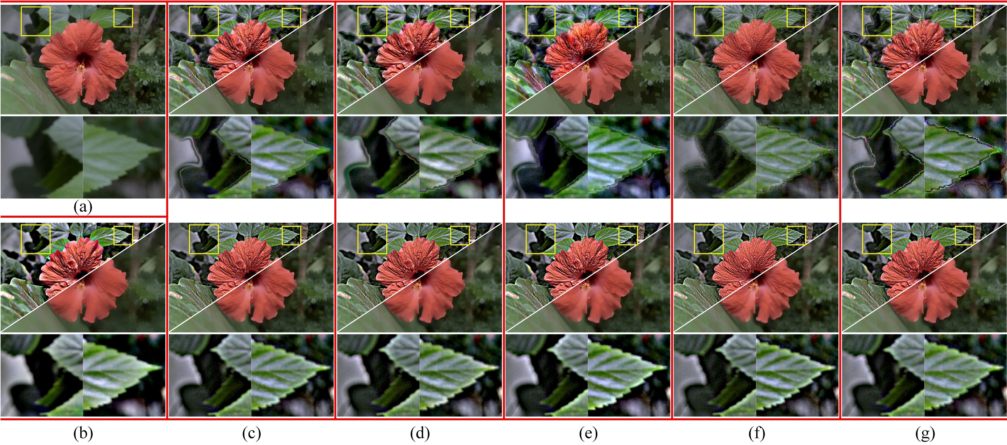
Flash/no-flash filtering was proposed by Petschnigg et al. [13] to smooth a noisy no-flash image with the guidance of the flash image. In [8], He et al. showed that gradient reversal artifacts also existed in the smoothed results of joint bilateral filter [13]. In our experiments, we find that results of adaptive manifold filter [7] and weighted median filter [20] also suffer from this problem. We show their results in the first row of Fig. 9 and illustrate gradient reversals in highlighted regions. However, these artifacts are properly eliminated by the proposed piecewise linear smoothing applied to these piecewise constant filters, which is similar to the result of guided image filter [8] in Fig. 9(b). When smoothing the gradients of no-flash images in the proposed method, we use the gradients of flash images as guidance images.
4 Conclusion
In this paper, we proposed a general framework to perform piecewise linear smoothing using several classical piecewise constant filters. The smoothed output images of the proposed method are based on a spatially piecewise linear model assumption which is different from the piecewise constant model assumption in most classical piecewise constant filters. The proposed method can properly handle with the problem of gradient reversal artifacts caused by the piecewise constant model assumption in several applications. In addition, the proposed method can further reduce the computational cost of accelerated methods which need to quantize image intensity values into different bins. Comprehensive experimental results in various applications show the effectiveness of the proposed method.
References
- [1] A. Buades, B. Coll, and J.-M. Morel. The staircasing effect in neighborhood filters and its solution. IEEE transactions on Image Processing, 15(6):1499–1505, 2006.
- [2] L. Dai, M. Yuan, F. Zhang, and X. Zhang. Fully connected guided image filtering. In Proceedings of the IEEE International Conference on Computer Vision, pages 352–360, 2015.
- [3] F. Durand and J. Dorsey. Fast bilateral filtering for the display of high-dynamic-range images. In ACM transactions on graphics (TOG), volume 21, pages 257–266. ACM, 2002.
- [4] Z. Farbman, R. Fattal, and D. Lischinski. Diffusion maps for edge-aware image editing. In ACM Transactions on Graphics (TOG), volume 29, page 145. ACM, 2010.
- [5] Z. Farbman, R. Fattal, D. Lischinski, and R. Szeliski. Edge-preserving decompositions for multi-scale tone and detail manipulation. In ACM Transactions on Graphics (TOG), volume 27, page 67. ACM, 2008.
- [6] E. S. Gastal and M. M. Oliveira. Domain transform for edge-aware image and video processing. In ACM Transactions on Graphics (ToG), volume 30, page 69. ACM, 2011.
- [7] E. S. Gastal and M. M. Oliveira. Adaptive manifolds for real-time high-dimensional filtering. ACM Transactions on Graphics (TOG), 31(4):33, 2012.
- [8] K. He, J. Sun, and X. Tang. Guided image filtering. IEEE transactions on pattern analysis and machine intelligence, 35(6):1397–1409, 2013.
- [9] A. Hosni, C. Rhemann, M. Bleyer, C. Rother, and M. Gelautz. Fast cost-volume filtering for visual correspondence and beyond. IEEE Transactions on Pattern Analysis and Machine Intelligence, 35(2):504–511, 2013.
- [10] Y. Li, L. Sharan, and E. H. Adelson. Compressing and companding high dynamic range images with subband architectures. In ACM transactions on graphics (TOG), volume 24, pages 836–844. ACM, 2005.
- [11] J. Lu, K. Shi, D. Min, L. Lin, and M. N. Do. Cross-based local multipoint filtering. In CVPR, 2012.
- [12] S. Paris and F. Durand. A fast approximation of the bilateral filter using a signal processing approach. European Conference on Computer Vision 2006, pages 568–580, 2006.
- [13] G. Petschnigg, R. Szeliski, M. Agrawala, M. Cohen, H. Hoppe, and K. Toyama. Digital photography with flash and no-flash image pairs. ACM transactions on graphics (TOG), 23(3):664–672, 2004.
- [14] L. I. Rudin, S. Osher, and E. Fatemi. Nonlinear total variation based noise removal algorithms. Physica D: Nonlinear Phenomena, 60(1-4):259–268, 1992.
- [15] R. Szeliski. Locally adapted hierarchical basis preconditioning. In ACM Transactions on Graphics (TOG), volume 25, pages 1135–1143. ACM, 2006.
- [16] X. Tan, C. Sun, and T. D. Pham. Multipoint filtering with local polynomial approximation and range guidance. In Proceedings of the IEEE Conference on Computer Vision and Pattern Recognition, pages 2941–2948. IEEE, 2014.
- [17] C. Tomasi and R. Manduchi. Bilateral filtering for gray and color images. In Computer Vision, 1998. Sixth International Conference on, pages 839–846. IEEE, 1998.
- [18] L. Xu, C. Lu, Y. Xu, and J. Jia. Image smoothing via gradient minimization. In ACM Transactions on Graphics (TOG), volume 30, page 174. ACM, 2011.
- [19] L. Xu, J. Ren, Q. Yan, R. Liao, and J. Jia. Deep edge-aware filters. In Proceedings of the 32nd International Conference on Machine Learning (ICML-15), pages 1669–1678, 2015.
- [20] Q. Zhang, L. Xu, and J. Jia. 100+ times faster weighted median filter (wmf). In Proceedings of the IEEE Conference on Computer Vision and Pattern Recognition, pages 2830–2837, 2014.