On large $q$ expansion in the Sachdev-Ye-Kitaev model

Abstract

We consider the Sachdev-Ye-Kitaev (SYK) model where interaction involves $q$ fermions at a time. We find the next order correction to the thermal two-point function in the large $q$ expansion. Using this result we find the next order correction to the SYK free energy.

I Introduction

The Sachdev-Ye-Kitaev (SYK) model is a quantum mechanical model of $N$ interacting Majorana fermions $\chi_{i}$, $i=1,\dots,N$ with the Hamiltonian Sachdev and Ye (1993); Kitaev :

$$H_{\textrm{SYK}_{q}}=(i)^{\frac{q}{2}}\sum_{1\leq i_{1}<i_{2}<\dots<i_{q}\leq N}J_{i_{1}\dots i_{q}}\chi_{i_{1}}\chi_{i_{2}}\dots\chi_{i_{q}}\,,$$ (1)

where $\{\chi_{i},\chi_{j}\}=\delta_{ij}$ and $J_{i_{1}\dots i_{q}}$ are random couplings drawn from a Gaussian distribution with zero mean and a width $\langle J_{i_{1}\dots i_{q}}^{2}\rangle=(q-1)!J^{2}/N^{q-1}$. One is usually interested in computing correlation functions, and particularly two-point function at temperature $T=1/\beta$:

$$G(\tau)=\langle T\chi(\tau)\chi(0)\rangle_{\beta}\,.$$ (2)

At the large $N$ limit only melonic Feynman diagrams contribute to the two-point function in the SYK model. These diagrams can be resummed and one obtains a non-perturbative Schwinger-Dyson equation:

$$G(i\omega_{n})^{-1}=-i\omega_{n}-\Sigma(i\omega_{n}),\quad\Sigma(\tau)=J^{2}G(\tau)^{q-1}\,,$$ (3)

where $G(i\omega_{n})=\int_{0}^{\beta}d\tau e^{i\omega_{n}\tau}G(\tau)$ and $\omega_{n}=2\pi\beta^{-1}(n+1/2)$. It is not possible to solve this equation analytically, but one can find solution in the infrared limit, where $\omega$ is small and the bare $-i\omega_{n}$-term in (3) can be neglected Sachdev and Ye (1993); Kitaev ; Maldacena and Stanford (2016); Parcollet and Georges (1999):

$$G_{c}(\tau)=b\Big{(}\frac{\pi}{\beta\sin\frac{\pi\tau}{\beta}}\Big{)}^{2/q}\textrm{sgn}(\tau)\,,$$ (4)

where $J^{2}b^{q}\pi=(1/2-1/q)\tan(\pi/q)$. Nevertheless it is still interesting to obtain some analytic approximation for $G(\tau)$ which interpolates both UV and IR regions. One way to proceed is to use the large $q$ expansion. The first order in $1/q$ was found in Maldacena and Stanford (2016). In this note we compute the next $1/q^{2}$ correction and argue that it improves the approximation significantly, such that it agrees with numerical results quite well.

At the next section we compute $1/q^{2}$ correction to the two-point function. Next we compare the large $q$ results and numerics. At the end we compute the large $q$ free energy and the coefficient of the Schwarzian action.

II Large $q$ two-point function

We consider the large $q$ ansatz for the two-point function Maldacena and Stanford (2016):

$$G(\tau)=\frac{1}{2}\textrm{sgn}(\tau)\Big{(}1+\frac{1}{q}g(\tau)+\frac{1}{q^{2}}h(\tau)+\dots\Big{)}\,.$$ (5)

For the self-energy (3) we find (we assume that $q$ is even)

$$\Sigma(\tau) =\frac{\mathcal{J}^{2}}{q}\textrm{sgn}(\tau)e^{g}\Big{(}1+\frac{1}{q}\big{(}h-g-\frac{1}{2}g^{2}\big{)}+\dots\Big{)}\,,$$ (6)

where a new coupling constant $\mathcal{J}^{2}=2^{1-q}qJ^{2}$ is introduced. From now on we work on the interval $\tau\in[0,\beta]$ and we can omit $\textrm{sgn}(\tau)$ in all formulas. Expanding $G(i\omega_{n})^{-1}$ in $1/q$ series up to $1/q^{2}$ term using (5) we obtain

$$G(i\omega_{n})^{-1}= -i\omega_{n}+\frac{1}{2q}\omega_{n}^{2}g(i\omega_{n})$$

$$+\frac{\omega_{n}^{2}}{2q^{2}}\Big{(}h(i\omega_{n})+\frac{i\omega_{n}}{2}g*g(i\omega_{n})\Big{)}\,,$$ (7)

where $g*g(i\omega_{n})\equiv\int_{0}^{\beta}d\tau e^{i\omega_{n}\tau}g^{2}(\tau)$. Then using the equations (3) and (6) and going back to the coordinate space we find differential equations for each order of $1/q$:

$$\partial_{\tau}^{2}g=2\mathcal{J}^{2}e^{g}\,,$$

$$\partial_{\tau}^{2}h=2\mathcal{J}^{2}e^{g}h+\frac{1}{2}\partial_{\tau}^{3}(g*g)-2\mathcal{J}^{2}e^{g}\big{(}g+\frac{1}{2}g^{2}\big{)}\,,$$ (8)

and the functions $g(\tau)$ and $h(\tau)$ satisfy the boundary conditions $g(0)=g(\beta)=0$ and $h(0)=h(\beta)=0$. Now we introduce a convenient variable $x=\frac{\pi v}{2}-\frac{\pi v\tau}{\beta}$. Then the first equation has the solution

$$g(x)=\log\Big{(}\frac{\cos\frac{\pi v}{2}}{\cos x}\Big{)}^{2},\quad\beta\mathcal{J}=\frac{\pi v}{\cos\frac{\pi v}{2}}\,.$$ (9)

Using this solution the second equation can be represented as

$$\Big{(}\partial_{x}^{2}-\frac{2}{\cos^{2}x}\Big{)}h(x)=$$

$$\quad\quad=-\frac{\pi v}{\beta}\frac{1}{2}\partial_{x}^{3}(g*g)-\partial_{x}^{2}g(x)\big{(}g(x)+\frac{1}{2}g^{2}(x)\big{)}\,.$$ (10)

The solution to this equation can be written as

$$h(x)= -\int_{-\frac{\pi v}{2}}^{\frac{\pi v}{2}}dy\mathcal{G}(x,y)\Big{(}\frac{\pi v}{\beta}\frac{1}{2}\partial_{y}^{3}(g*g)$$

$$\qquad\qquad+\partial_{y}^{2}g(y)\big{(}g(y)+\frac{1}{2}g^{2}(y)\big{)}\Big{)}\,,$$ (11)

where the Green’s function $\mathcal{G}(x,y)$ obeys the equation

$$\Big{(}\partial_{x}^{2}-\frac{2}{\cos^{2}x}\Big{)}\mathcal{G}(x,y)=\delta(x-y)\,$$ (12)

with the boundary conditions $\mathcal{G}(-\frac{\pi v}{2},y)=\mathcal{G}(\frac{\pi v}{2},y)=0$. One can solve this equation and obtain an explicit formula for the Green’s function

$$\mathcal{G}(x,y)=\frac{1}{2V}(\tan x_{<}(V+x_{<})+1)(\tan x_{>}(V-x_{>})-1)\,,$$ (13)

where $V\equiv\frac{\pi v}{2}+\cot\frac{\pi v}{2}$ and $x_{>}\equiv\max(x,y)$ and $x_{<}\equiv\min(x,y)$. Computing the convolution

$$\frac{\pi v}{\beta}\frac{1}{2}\partial_{x}^{3}(g*g)=$$

$$=2\partial_{x}\Big{(}g(x)\big{(}\cot(\frac{\pi v}{2}+x)-\cot(\frac{\pi v}{2}-x)\big{)}\Big{)}-4\,,$$ (14)

and using the explicit formula for the Green’s function (13) we obtain from (11)

$$h(x)=\frac{1}{2}g^{2}(x)-2\ell(x)-4\Big{(}\tan x\int_{0}^{x}dy\ell(y)+1\Big{)}$$

$$\quad+4\frac{1+x\tan x}{1+\frac{\pi v}{2}\tan\frac{\pi v}{2}}\Big{(}\tan\frac{\pi v}{2}\int_{0}^{\frac{\pi v}{2}}dy\ell(y)+1\Big{)}\,,$$ (15)

where $\ell(x)\equiv g(x)-e^{-g(x)}\textrm{Li}_{2}(1-e^{g(x)})$ and $g(x)$ is given in (9). One can compute explicitly the integral (formulas from Davydychev and Kalmykov (2004) are useful)

$$\int_{0}^{\frac{\pi v}{2}}dy\ell(y)=-\frac{\pi^{2}v^{2}}{24\cos^{2}\frac{\pi v}{2}}(\pi v+3\sin\pi v)\,.$$ (16)

III Comparison with numerical results

In this section we compare the large $q$ result with the numerical solution of the Schwinger-Dyson equation (3). In general we expect the large $q$ formula to work well when $|g(\tau)|\ll q$ and $|h(\tau)|\ll q^{2}$. These inequalities are fulfilled when $\beta\mathcal{J}\ll\pi e^{q/2}$.

Looking at the explicit formula (15) it is tempting to exponentiate the result and to introduce an exponentiated large $q$ two-point function

$$G(\tau)=\frac{1}{2}\textrm{sgn}(\tau)\exp\Big{(}\frac{1}{q}g+\frac{1}{q^{2}}(h-\frac{1}{2}g^{2})\Big{)}\,,$$ (17)

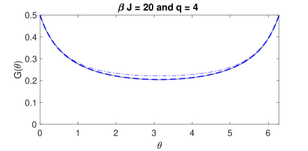
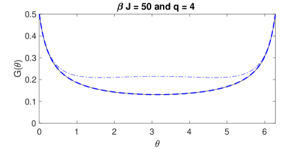
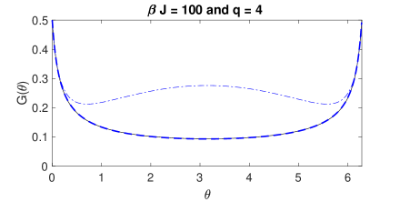
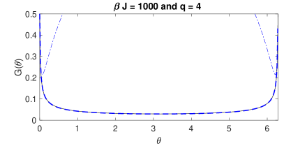
which is equivalent to (5) up to order $1/q^{2}$. We plot numerical and the large $q$ results for $q=4$ and different values of $\beta J$ in figure 1. We can see that the exponentiated result works very precisely even for large $\beta J$, whereas the large $q$ answer (5) deviates significantly from numerics at large $\beta J$.

Figure 1: (Color online) Plots of the numerical solution and the large $q$ approximations for $G(\theta)$, $\theta=2\pi\tau/\beta$ at $\beta J=20,50,100,1000$ and $q=4$. The black solid line is the numerical solution for the Schwinger-Dyson equation (3). The blue dash-dotted line is the large $q$ approximation (5) with $1/q^{2}$ term. The blue dashed line is the exponentiated two-point function (17).

IV Large $q$ free energy

The leading large $N$ approximation to the free energy in the SYK model is Kitaev ; Sachdev (2015)

$$-\frac{\beta F}{N}=\log\textrm{Pf}(\partial_{\tau}-\Sigma)$$

$$\qquad-\frac{1}{2}\int_{0}^{\beta}d\tau_{1}d\tau_{2}\Big{(}\Sigma(\tau_{12})G(\tau_{12})-\frac{J^{2}}{q}G(\tau_{12})^{q}\Big{)}\,.$$ (18)

To avoid evaluating the Pfaffian it is convenient to differentiate the free energy by $J\partial_{J}$ Maldacena and Stanford (2016)

$$J\partial_{J}(-\beta F/N) =-\frac{\beta}{q}\partial_{\tau}G|_{\tau\to+0}$$

$$=\frac{\pi v}{2q}\big{(}\frac{1}{q}\partial_{x}g+\frac{1}{q^{2}}\partial_{x}h\big{)}|_{x\to\frac{\pi v}{2}}\,,$$ (19)

where from (9) and (15) we find

$$\partial_{x}g|_{x\to\frac{\pi v}{2}}=2\tan\frac{\pi v}{2}\,,$$

$$\partial_{x}h|_{x\to\frac{\pi v}{2}}=\frac{4}{1+\frac{\pi v}{2}\tan\frac{\pi v}{2}}\Big{(}\frac{\pi v}{2}$$

$$\quad\qquad-\tan\frac{\pi v}{2}(1+\frac{\pi v}{2}\tan\frac{\pi v}{2})-\int_{0}^{\frac{\pi v}{2}}dy\ell(y)\Big{)}\,.$$ (20)

Next, using (16) and

$$J\partial_{J}=\frac{v\partial_{v}}{1+\frac{\pi v}{2}\tan\frac{\pi v}{2}}\,,$$ (21)

we can integrate back and obtain $-\beta F/N=\frac{1}{2}\log 2+\frac{1}{q^{2}}F_{1/q^{2}}+\frac{1}{q^{3}}F_{1/q^{3}}+\dots$, where

$$F_{1/q^{2}}(v)=\pi v\Big{(}\tan\frac{\pi v}{2}-\frac{\pi v}{4}\Big{)}\,,$$

$$F_{1/q^{3}}(v)=\pi v\Big{(}\pi v-2\tan\frac{\pi v}{2}\big{(}1-\frac{\pi^{2}v^{2}}{12}\big{)}\Big{)}\,.$$ (22)

Expanding the free energy at strong coupling by using that

$$v=1-\frac{2}{\beta\mathcal{J}}+\frac{4}{(\beta\mathcal{J})^{2}}-\frac{(24+\pi^{2})}{3(\beta\mathcal{J})^{3}}+\dots\,,$$ (23)

we find

$$-\frac{\beta F}{N}= \beta\mathcal{J}\Big{(}\frac{1}{q^{2}}-\frac{12-\pi^{2}}{6q^{3}}\Big{)}+\Big{(}\frac{1}{2}\log 2-\frac{\pi^{2}}{4q^{2}}+\frac{\pi^{2}}{3q^{3}}\Big{)}$$

$$+\frac{1}{\beta\mathcal{J}}\Big{(}\frac{\pi^{2}}{2q^{2}}-\frac{\pi^{2}(\pi^{2}+12)}{12q^{3}}\Big{)}$$

$$+\frac{1}{(\beta\mathcal{J})^{2}}\Big{(}-\frac{\pi^{2}}{q^{2}}+\frac{\pi^{2}(5\pi^{2}+24)}{9q^{3}}\Big{)}+\dots,$$ (24)

where the first three terms are the ground state energy, the zero-temperature entropy and the temperature dependent correction to the entropy. The zero temperature entropy coincides with the large $q$ expansion of the formula Kitaev ; Georges et al. (2001)

$$\frac{S_{0}}{N} =\frac{1}{2}\log 2-\int_{0}^{1/q}dx\pi(\frac{1}{2}-x)\tan\pi x\,.$$ (25)

The last term in (24) agrees with the formula reported in Cotler et al. (2017); Jevicki and Suzuki (2016); Kitaev and Suh (2017).

Using the result (24) one can find the coefficient of the Schwarzian action. The Schwarzian action, which governs the low energy dynamics of the SYK model is given by the formula Maldacena and Stanford (2016); Maldacena et al. (2016); Engels y et al. (2016); Jensen (2016); Jevicki et al. (2016)

$$S=-N\frac{\alpha_{S}}{\mathcal{J}}\int d\tau\{f,\tau\},\quad\{f,\tau\}\equiv\frac{f^{\prime\prime\prime}}{f^{\prime}}-\frac{3}{2}\Big{(}\frac{f^{\prime\prime}}{f^{\prime}}\Big{)}^{2}\,,$$ (26)

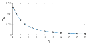
where the coefficient $\alpha_{S}$ depends on $q$. This coefficient is related to the finite temperature correction to the free energy, so at large $q$ using (24) we find

$$-\frac{\beta F}{N}\supset\frac{2\pi^{2}\alpha_{S}}{\beta\mathcal{J}}=\frac{1}{\beta\mathcal{J}}\Big{(}\frac{\pi^{2}}{2q^{2}}-\frac{\pi^{2}(\pi^{2}+12)}{12q^{3}}+\dots\Big{)}\,.$$ (27)

At $q=2$ one has $\alpha_{S}=\frac{1}{24\pi}$. Using asymptotics for $\alpha_{S}$ at $q=\infty$ and $q=2$

$$\alpha_{S}(q)=\begin{cases}\frac{1}{24\pi}+\dots\,,\;\;\qquad\qquad q\to 2\\ \frac{1}{4q^{2}}-\frac{\pi^{2}+12}{24q^{3}}+\dots,\quad q\to\infty\end{cases}$$ (28)

we obtain two-sided Pade approximant:

$$\textrm{Pade}_{[3,1]}:\;\;\alpha_{S}(q)=\frac{\pi^{2}-18\pi+24+3(3\pi-2)q}{6q^{2}\left(\pi^{3}+8+2(3\pi-2)q\right)}\,.$$ (29)

We note that one can improve approximation by using more terms near $q=2$ Jevicki and Suzuki (2016). We plotted Pade approximation and numerical results adapted from Maldacena and Stanford (2016) in figure 2. We see that the Pade approximation is very close to numerics.

Figure 2: (Color online) Plot of $\alpha_{S}$ as a function of $q$. The black circles correspond to numerical results adapted from Maldacena and Stanford (2016). The blue solid line corresponds to the two-sided Pade approximation (29).

V Conclusions

It would be interesting to generalize the result of this article to other SYK-type models, discussed in Gross and Rosenhaus (2017); Davison et al. (2017); Gu et al. (2017); Fu et al. (2017). Especially it would be interesting to compute the thermalization time using large $q$ solution for the SYK models discussed in Eberlein et al. (2017).

It is also interesting to develop $1/q$ expansion for the higher dimensional SYK models Berkooz et al. (2017); Turiaci and Verlinde (2017); Murugan et al. (2017); Giombi et al. (2017); Prakash and Sinha (2017) where the stability of the large $N$ limit is unclear.

The large $q$ approximation to the two-point function can be used as well in studying tensor models Witten (2016); Gurau (2017); Klebanov and Tarnopolsky (2017). Even though the general $q$ melonic tensor interaction have some ambiguities Jepsen ; Klebanov and Tarnopolsky (2017), one can just formally consider large $q$ generalization of the Schwinger-Dyson equation.

G.T. would like to thank Yingfei Gu, Igor Klebanov, Subir Sachdev and Douglas Stanford for useful comments. Also G.T. thanks Douglas Stanford for providing numerical results for $\alpha_{S}$ from Maldacena and Stanford (2016). This research was supported by the MURI grant W911NF-14-1-0003 from ARO and by DOE grant de-sc0007870.