Time-Delay Origins of Fundamental Tradeoffs Between
Risk of Large Fluctuations and Network Connectivity

Christoforos Somarakis, Yaser Ghaedsharaf, Nader Motee The authors are with the Department of Mechanical Engineering and Mechanics, Lehigh University, Bethlehem, PA, 18015, USA. {csomarak,ghaedsharaf,motee}@lehigh.edu
Abstract

For the class of noisy time-delay linear consensus networks, we obtain explicit formulas for risk of large fluctuations of a scalar observable as a function of Laplacian spectrum and its eigenvectors. It is shown that there is an intrinsic tradeoff between risk and effective resistance of the underlying coupling graph of the network. The main implication is that increasing network connectivity, increases the risk of large fluctuations. For vector-valued observables, we obtain computationally tractable lower and upper bounds for joint risk measures. Then, we study behavior of risk measures for networks with specific graph topologies and show how risk scales with network size.

1 Introduction

The notion of systemic risk describes fragility in interconnected networks that can result in global or cascading failures due to either relatively small disturbances at the subsystem level or larger and more malicious types of disruptions affecting the whole network. The challenges of dealing with risk spread through many areas of engineering and economy [1, 2, 3, 6, 11, 31]. Modern networked control systems bear innate complexities in their structure and evolving dynamics. There are numerous networks, which are playing major roles in fabrics of our society, that are susceptible to exogenous stochastic uncertainties and disturbances. Examples include platoon of autonomous vehicles in highways, synchronous power networks with integrated renewable sources, water supply networks, interconnected networks of financial institutions, and air traffic networks. The recent crisis show specific vulnerabilities of modern networks due to weaknesses in their structures, e.g., air traffic congestion, power outages, the 2008 financial crisis, and other major disruptions. The costly and severe in magnitude outcomes of these network-related crisis motivate risk-oriented analysis and synthesis of networked control systems.

There are some recent lines of research that are close in spirit to the subject of this paper. In [6], the authors introduce novel concepts of resilience for dynamic flow networks, where they study robustness of such network with respect to perturbations that reduce the flow functions on the links of the network. They also discuss a situation in which imposing finite density constraints on the links may result in cascaded failures. Other related works [4, 21, 36, 37] utilize performance measures based on 2subscript2\mathcal{H}_{2}-norm to quantify quality of noise propagation in noisy linear consensus networks. The focus of these works are on linear consensus networks with no time delay. In [38, 35], the authors introduce a class of spectral systemic performance measures (which includes psubscript𝑝\mathcal{H}_{p}-norms as its special case) to synthesize networks through growing and sparsification of links in noisy linear consensus networks in absence of time delay. In all these papers, performance measures assess holistic and macroscopic features of the networks, such as total deviation from average or uncertainty volume of the output. In this paper, we show that exogenous uncertainties along with time delay creates unorthodox behaviors in microscopic level that cannot be captured by the existing performance measures in literature.

The class of time-delay linear consensus model (6) has been previously studied within different disciplines [16, 17, 20, 23, 13, 14]. In [16], the authors obtain expressions for the average size of fluctuations using modal behavior of the network. They also show how extreme fluctuations scale with network size and argue that distribution of those nodes with highest fluctuation takes specific forms. The focus of [17] is on synchronizability threshold and the scaling behavior of the width of the synchronization for linear consensus systems with uniform and multiple time delays, where their results and analysis are heavily relied on numerical simulations. Reference [23] proposes a method to study systems with multiple delays (scalar and multidimensional) in the presence of additive noise. Using Laplace transform, they obtain an integral formula for statistics of the state variables without providing closed form solutions for the integrals. Their results are applied to first and second order consensus networks with multiple delays and complete (all-to-all) graph topology. Extensive numerical solutions to draw conclusions are evident in all these works. In this paper, we adopt a rigorous terminology and develop tools based on notions of risk to quantify and measure the tendency of noisy time-delay linear consensus networks towards exhibiting undesirable systemic events (e.g., large fluctuations and violating critical constraints). Our analysis is based on the fact that a time-delay linear consensus network can be decomposed into many one-dimensional systems and then analyzed using tools developed in [20, 13, 14].

Systemic risk as a tool for decision making under uncertainty has been initially employed to study uncertainties in financial markets [2, 3, 11, 31, 32]. More recently, cascading failures in interconnected financial institutes have been studied [1, 11]. In [41, 40], the notion of value-at-risk has been applied to calculate probability of large fluctuations due to external disturbances in linear consensus networks with no time delay. The present work is an outgrowth of [40] and [41] in a number of ways. At first, we introduce and analyze two types of risk measures to assess possibility of large fluctuations in networks: one gauge risk in probability and the other one in expectation w.r.t. a utility (cost) function. By exploiting functional properties of risk measures, such as (quasi-) convexity and monotonicity, we calculate explicit formulas for them w.r.t. scalar network observables and show that these individual risk measures are spectral functions of Laplacian eigenvalues and eigenvectors. Furthermore, it is shown that the risk measures are not monotone functions of Laplacian eigenvalues, i.e., increasing connectivity (through adding new feedback interconnections or increasing feedback gains) may increase risk of large fluctuations and sparsification (eliminating existing feedback loops) may decrease risk of large fluctuations. We do not observe this peculiar behavior when there is no time delay. In addition to the fundamental limits reported to [40], we characterize several Heisenberg-like inequalities and reveal intrinsic tradeoff between the risk measure and network connectivity. Our results assert that in presence of time delay more connectivity results in higher risk of large fluctuations that in turn may lead to violation of critical constraints and network fragility. Finally, we extend our risk analysis to multiple network observables. In this case, the risk measures take vector values and one needs to calculate joint risk measures. In general, obtaining explicit closed form formulas for the joint risk measures is nearly impossible. However, one can employ numerical algorithms to compute values of such joint risk measures [12]. To tackle this challenge, we obtain tight lower and upper bounds for the joint risk measures and show that joint risk measures depend on the vector of individual risk measures, where we know how to calculate them explicitly. The big advantage of our bounds is that they are computationally tractable. Finally, we investigate behavior of risk for networks with particular graph topologies and show how the risk measures scale with network size. Several numerical examples support our theoretical findings. The proofs of all technical results, in this work, are placed in the Appendix.

2 Preliminaries

Throughout the paper, plain and bold lowercase letters are reserved for scalar-valued and vector-valued variables, respectively. The n𝑛n-dimensional Euclidean space with elements 𝐳=(z1,,zn)T𝐳superscriptsubscript𝑧1subscript𝑧𝑛𝑇\mathbf{z}=(\hskip 1.42271ptz_{1},\hskip 1.42271pt\dots\hskip 1.42271pt,z_{n}\hskip 1.42271pt)^{T} is denoted by nsuperscript𝑛\mathbb{R}^{n}. The set of standard Euclidean basis for nsuperscript𝑛{\mathbb{R}}^{n} is {𝐞1,,𝐞n}subscript𝐞1subscript𝐞𝑛\{\mathbf{e}_{1},\ldots,\mathbf{e}_{n}\}. The nonnegative orthant cone is defined by

+n={𝐳n|zi0for alli=1,,n}.subscriptsuperscript𝑛conditional-set𝐳superscript𝑛formulae-sequencesubscript𝑧𝑖0for all𝑖1𝑛{\mathbb{R}}^{n}_{+}=\big{\{}\mathbf{z}\in{\mathbb{R}}^{n}\leavevmode\nobreak\ \big{|}\leavevmode\nobreak\ z_{i}\geq 0\leavevmode\nobreak\ \leavevmode\nobreak\ \textrm{for all}\leavevmode\nobreak\ \leavevmode\nobreak\ i=1,\ldots,n\big{\}}.

For 𝒙,𝒛n𝒙𝒛superscript𝑛\boldsymbol{x},\boldsymbol{z}\in{\mathbb{R}}^{n}, relation 𝒙𝒛precedes-or-equals𝒙𝒛\boldsymbol{x}\preceq\boldsymbol{z} holds iff 𝒛𝒙+n𝒛𝒙subscriptsuperscript𝑛\boldsymbol{z}-\boldsymbol{x}\in{\mathbb{R}}^{n}_{+}, and 𝒙𝒛precedes𝒙𝒛\boldsymbol{x}\prec\boldsymbol{z} iff all elements of 𝒛𝒙𝒛𝒙\boldsymbol{z}-\boldsymbol{x} are strictly positive. The Euclidean vector and induced matrix norms is represented by \|\cdot\|, while absolute value operation for vectors is defined element-wise, i.e., |𝐳|=[|z1|,,|zn|]T𝐳superscriptsubscript𝑧1subscript𝑧𝑛𝑇|\mathbf{z}|=[\hskip 1.42271pt|z_{1}|,\hskip 1.42271pt\ldots\hskip 1.42271pt,|z_{n}|\hskip 1.42271pt]^{T}. The n×1𝑛1n\times 1 vector of all ones is shown by 𝟏nsubscript1𝑛\mathbf{1}_{n} and the n×n𝑛𝑛n\times n centering matrix is defined as Mn:=In1n𝟏n𝟏nTassignsubscript𝑀𝑛subscript𝐼𝑛1𝑛subscript1𝑛superscriptsubscript1𝑛𝑇M_{n}:=I_{n}-\frac{1}{n}\mathbf{1}_{n}\mathbf{1}_{n}^{T}, where 𝐦isubscript𝐦𝑖\mathbf{m}_{i} is the i𝑖i’th column of Mnsubscript𝑀𝑛M_{n}. Representation of a vector in nsuperscript𝑛\mathbb{R}^{n} with respect to linearly independent columns of matrix Q=[𝐪1||𝐪n]𝑄delimited-[]subscript𝐪1subscript𝐪𝑛Q=[\mathbf{q}_{1}\leavevmode\nobreak\ |\leavevmode\nobreak\ \dots\leavevmode\nobreak\ |\leavevmode\nobreak\ \mathbf{q}_{n}] is shown by 𝐳Q=[z1Q,,znQ]Tsuperscript𝐳𝑄superscriptsuperscriptsubscript𝑧1𝑄superscriptsubscript𝑧𝑛𝑄𝑇\mathbf{z}^{Q}=[\hskip 1.42271ptz_{1}^{Q},\hskip 1.42271pt\dots\hskip 1.42271pt,z_{n}^{Q}\hskip 1.42271pt]^{T}, where ziQ=𝐪iT𝐳superscriptsubscript𝑧𝑖𝑄superscriptsubscript𝐪𝑖𝑇𝐳z_{i}^{Q}=\mathbf{q}_{i}^{T}\mathbf{z}.

Algebraic Graph Theory: A weighted graph is the triple 𝒢=(𝒱,,w)𝒢𝒱𝑤\mathcal{G}=({\mathcal{V}},\mathcal{E},w), where 𝒱𝒱{\mathcal{V}} is the set of nodes, \mathcal{E} is the set of links (edges), and w:+:𝑤subscriptw:\mathcal{E}\rightarrow\mathbb{R}_{+} is the weight function of the graph that assigns a real number to every link.

Assumption 1.

For every pair of nodes i,j𝒱𝑖𝑗𝒱i,j\in\mathcal{V}, we assume: (i) nonnegativity of link weights, i.e., w(i,j)0𝑤𝑖𝑗0w(i,j)\geq 0 (ii) indirectness of links, i.e., w(i,j)=w(j,i)𝑤𝑖𝑗𝑤𝑗𝑖w(i,j)=w(j,i), and (iii) simpleness, i.e., w(j,j)=0𝑤𝑗𝑗0w(j,j)=0. Moreover, this paper only considers connected graphs.

Let us denote kij=w(i,j)subscript𝑘𝑖𝑗𝑤𝑖𝑗k_{ij}=w(i,j) for every i,j𝒱𝑖𝑗𝒱i,j\in{\mathcal{V}}. The Laplacian matrix of graph 𝒢𝒢{\mathcal{G}} is an n×n𝑛𝑛n\times n matrix L=[lij]𝐿delimited-[]subscript𝑙𝑖𝑗L=[l_{ij}] whose elements are defined as

lij:={kijifijki1++kinifi=j.assignsubscript𝑙𝑖𝑗casessubscript𝑘𝑖𝑗if𝑖𝑗missing-subexpressionmissing-subexpressionmissing-subexpressionsubscript𝑘𝑖1subscript𝑘𝑖𝑛if𝑖𝑗\displaystyle l_{ij}:=\left\{\begin{array}[]{ccc}-k_{ij}&\textrm{if}&i\neq j\\ &&\\ k_{i1}+\ldots+k_{in}&\textrm{if}&i=j\end{array}\right.. (1)

Laplacian matrix of a graph is symmetric and positive semi-definite. Our connectivity assumption implies that only the smallest Laplacian eigenvalue is equal to zero and all other ones are strictly positive, i.e., 0=λ1<λ2λn0subscript𝜆1subscript𝜆2subscript𝜆𝑛0=\lambda_{1}<\lambda_{2}\leq\ldots\leq\lambda_{n}. The eigenvector of L𝐿L corresponding to λksubscript𝜆𝑘\lambda_{k} is denoted by 𝐪ksubscript𝐪𝑘\mathbf{q}_{k}. By letting Q=[𝐪1||𝐪n]𝑄delimited-[]subscript𝐪1subscript𝐪𝑛Q=[\hskip 1.42271pt\mathbf{q}_{1}\leavevmode\nobreak\ |\leavevmode\nobreak\ \dots\leavevmode\nobreak\ |\leavevmode\nobreak\ \mathbf{q}_{n}\hskip 1.42271pt], it follows that L=QΛQT𝐿𝑄Λsuperscript𝑄𝑇L=Q\Lambda Q^{T} with Λ=diag[0,λ2,,λn]Λdiag0subscript𝜆2subscript𝜆𝑛\Lambda=\mathrm{diag}[\hskip 1.42271pt0,\hskip 1.42271pt\lambda_{2},\hskip 1.42271pt\ldots\hskip 1.42271pt,\hskip 1.42271pt\lambda_{n}\hskip 1.42271pt]. We normalize the Laplacian eigenvectors such that Q𝑄Q becomes an orthogonal matrix, i.e., QTQ=QQT=Insuperscript𝑄𝑇𝑄𝑄superscript𝑄𝑇subscript𝐼𝑛Q^{T}Q=QQ^{T}=I_{n} with 𝐪1=1n𝟏nsubscript𝐪11𝑛subscript1𝑛\mathbf{q}_{1}=\frac{1}{\sqrt{n}}\mathbf{1}_{n}.

Remark 1.

Suppose that Ensubscript𝐸𝑛E_{n} is the n×n𝑛𝑛n\times n diagonal matrix that is obtained by setting element of (1,1)11(1,1) of Insubscript𝐼𝑛I_{n} to zero. For an n×n𝑛𝑛n\times n unitary matrix Q𝑄Q, standard graph theory results are: Mn=QEnQTsubscript𝑀𝑛𝑄subscript𝐸𝑛superscript𝑄𝑇M_{n}=QE_{n}Q^{T} and BnTBn=nMn=nQEnQTsuperscriptsubscript𝐵𝑛𝑇subscript𝐵𝑛𝑛subscript𝑀𝑛𝑛𝑄subscript𝐸𝑛superscript𝑄𝑇B_{n}^{T}B_{n}=nM_{n}=nQE_{n}Q^{T}, where Bnsubscript𝐵𝑛B_{n} is the n(n1)2×n𝑛𝑛12𝑛\frac{n(n-1)}{2}\times n complete incidence matrix.

The notion of effective resistance is a widely used metric to measure how strongly a graph is connected in the context of graph theory [19, 25, 37]. The effective resistance between every pair of nodes i𝑖i and j𝑗j of a graph can be interpreted as the voltage difference between terminals i𝑖i and j𝑗j if we replace every link with an electrical resistance (whose value is equal to that link’s weight) and let unit current source to be applied between the two nodes; we refer to [8, 19] for more information. The total effective resistance is the sum of all effective resistances over all distinct pair of nodes in 𝒢𝒢\mathcal{G} and is equal to [19]

Ξ𝒢=ni=2nλi1,subscriptΞ𝒢𝑛superscriptsubscript𝑖2𝑛superscriptsubscript𝜆𝑖1\Xi_{\mathcal{G}}=n\sum_{i=2}^{n}\lambda_{i}^{-1}, (2)

where λ2,,λnsubscript𝜆2subscript𝜆𝑛\lambda_{2},\ldots,\lambda_{n} are the non-zero Laplacian eigenvalues.

Probability Theory: A complete filtered probability space is the quadruple (Ω,,{t}t0,)Ωsubscriptsubscript𝑡𝑡0(\Omega,\mathcal{F},\{\mathcal{F}_{t}\}_{t\geq 0},\mathbb{P}), where {t}t0subscriptsubscript𝑡𝑡0\{\mathcal{F}_{t}\}_{t\geq 0} is the filtration of a vector-valued standard Brownian motion {𝐰t}t0subscriptsubscript𝐰𝑡𝑡0\{\mathbf{w}_{t}\}_{t\geq 0}, with 𝐰t=(w1(t),,wn(t))Tsubscript𝐰𝑡superscriptsubscript𝑤1𝑡subscript𝑤𝑛𝑡𝑇\mathbf{w}_{t}=\big{(}w_{1}(t),\ldots,w_{n}(t)\big{)}^{T} constructed out of n𝑛n independent scalar Brownian motions. The space of all \mathcal{F}-measurable, qsuperscript𝑞\mathbb{R}^{q}-valued random variables with finite second moment is denoted by 𝕃2(q)superscript𝕃2superscript𝑞\mathbb{L}^{2}(\mathbb{R}^{q}). The stochastic process 𝐲={𝐲t}t𝐲subscriptsubscript𝐲𝑡𝑡\mathbf{y}=\{\mathbf{y}_{t}\}_{t\in\mathbb{R}} is {t}subscript𝑡\{\mathcal{F}_{t}\}-adapted if 𝐲tsubscript𝐲𝑡\mathbf{y}_{t} is tsubscript𝑡\mathcal{F}_{t}-measurable for t0𝑡0t\geq 0. The multi-variable normal distribution is denoted by 𝒩(𝝁,Σ)𝒩𝝁Σ\mathcal{N}(\boldsymbol{\mu},\Sigma), where 𝝁q𝝁superscript𝑞\boldsymbol{\mu}\in\mathbb{R}^{q} is the expected value and ΣΣ\Sigma is the q×q𝑞𝑞q\times q positive semi-definite covariance matrix. A random variable 𝐲𝒩(𝝁,Σ)similar-to𝐲𝒩𝝁Σ\mathbf{y}\sim\mathcal{N}(\boldsymbol{\mu},\Sigma) attains a density function if and only if ΣΣ\Sigma is positive definite. The error function is denoted as

erf(z)=1πzzet2𝑑t.erf𝑧1𝜋superscriptsubscript𝑧𝑧superscript𝑒superscript𝑡2differential-d𝑡\mathrm{erf}(z)=\frac{1}{\sqrt{\pi}}\int_{-z}^{z}e^{-t^{2}}\,dt.

For fixed ε(0,1)𝜀01\varepsilon\in(0,1), the following quantity is introduced for the sake of convenience:

Sε(α)=inf{δ+|1πδ2αδet2𝑑t1ε}subscript𝑆𝜀𝛼infimumconditional-set𝛿subscript1𝜋superscriptsubscript𝛿2𝛼𝛿superscript𝑒superscript𝑡2differential-d𝑡1𝜀S_{\varepsilon}(\alpha)=\inf\bigg{\{}\delta\in\mathbb{R}_{+}\leavevmode\nobreak\ \bigg{|}\leavevmode\nobreak\ \frac{1}{\sqrt{\pi}}\int_{-\delta-2\alpha}^{\delta}e^{-t^{2}}\,dt\geq 1-\varepsilon\bigg{\}} (3)

and Sε(0)=inf{δ+|erf(δ)1ε}S_{\varepsilon}(0)=\inf\big{\{}\delta\in\mathbb{R}_{+}\leavevmode\nobreak\ |\leavevmode\nobreak\ \leavevmode\nobreak\ \mathrm{erf}(\delta)\geq 1-\varepsilon\big{\}}.

3 Problem Statement

We consider the class of time-delay linear consensus networks that has found wide applications in engineering (e.g., clock synchronization in sensor networks, rendezvous in a space or time, and heading alignment in swarm robotics) and social sciences (e.g., agreement in opinion networks); we refer to [30, 28] for more details. As a motivational application, we discuss a cooperative rendezvous problem where the control objective of a team of agents (e.g., ground vehicles or quadcopters) is to meet simultaneously at a pre-specified location known to all agents111Rendezvous in space is very similar to rendezvous in time by switching the role of time and location in the above explanation.. In this rendezvous problem agents do not have a priori knowledge of the meeting time as it may have to be adjusted in response to unexpected emergencies or exogenous uncertainties (see [30] for a detailed discussion). Thus, all agents should agree on a rendezvous time by achieving consensus. This is usually done by each agent creating a state variable, say xisubscript𝑥𝑖x_{i}\in{\mathbb{R}}, that represents its estimation of the rendezvous time. Each agent’s initial estimate is set to a preferred time at which it would be able to rendezvous with other agents. The rendezvous (more generally consensus) dynamics for each agent evolves in time according to the following stochastic differential equation

dxi(t)=ui(t)dt+bdwi(t)𝑑subscript𝑥𝑖𝑡subscript𝑢𝑖𝑡𝑑𝑡𝑏𝑑subscript𝑤𝑖𝑡d{x}_{i}(t)=u_{i}(t)dt+b\hskip 1.42271ptdw_{i}(t) (4)

for all i=1,,n𝑖1𝑛i=1,\ldots,n. Each agent’s control input is uisubscript𝑢𝑖u_{i}\in{\mathbb{R}}. The source of uncertainty is diffused in the network as additive stochastic noise, the magnitude of which is uniformly scaled by the diffusion b𝑏b\in\mathbb{R}. The impact of uncertain environments on dynamics of agents are modeled by independent Brownian motions w1,,wnsubscript𝑤1subscript𝑤𝑛w_{1},\ldots,w_{n}. In real-world situations, each agent experiences a time delay in accessing, computing, or sharing its own state information with itself and other neighboring agents [30]. It is assumed222This assumption has been widely used by other researchers as it allows analytical derivations of formulas. For rendezvous in time, it is a common practice in robotics labs to use identical communication modules for all agents, which results in a uniform communication time delay. Moreover, in other related applications such as heading alignments, rendezvous in space, and velocity control of agents using a Motion Capture (MoCap) system to observe their spatial locations in indoor labs [22, 24, 39], all agents experience an identical time delay to access data through MoCap system. that all agents experience an identical time delay that is equal to a nonnegative number τ𝜏\tau. The control inputs are determined via a negotiation process by forming a linear consensus network over a communication graph using the following feedback law

ui(t)=j=1nkij(xj(tτ)xi(tτ)),subscript𝑢𝑖𝑡superscriptsubscript𝑗1𝑛subscript𝑘𝑖𝑗subscript𝑥𝑗𝑡𝜏subscript𝑥𝑖𝑡𝜏u_{i}(t)\leavevmode\nobreak\ =\leavevmode\nobreak\ \sum_{j=1}^{n}k_{ij}\big{(}x_{j}(t-\tau)-x_{i}(t-\tau)\big{)}, (5)

where kijsubscript𝑘𝑖𝑗k_{ij} are non-negative feedback gains. Let us denote the state vector by 𝐱t=(x1(t),,xn(t))Tsubscript𝐱𝑡superscriptsubscript𝑥1𝑡subscript𝑥𝑛𝑡T\mathbf{x}_{t}=\big{(}x_{1}(t),\ldots,x_{n}(t)\big{)}^{\rm T} and the vector of exogenous disturbance by 𝐰t=(w1(t),,wn(t))Tsubscript𝐰𝑡superscriptsubscript𝑤1𝑡subscript𝑤𝑛𝑡T\mathbf{w}_{t}=\big{(}w_{1}(t),\ldots,w_{n}(t)\big{)}^{\rm T}. The dynamics of the resulting closed-loop network can be cast as a linear consensus network that is governed by the stochastic delay differential equation

d𝐱t=L𝐱tτdt+Bd𝐰t𝑑subscript𝐱𝑡𝐿subscript𝐱𝑡𝜏𝑑𝑡𝐵𝑑subscript𝐰𝑡d\mathbf{x}_{t}=-L\hskip 1.42271pt\mathbf{x}_{t-\tau}\hskip 1.42271ptdt+B\hskip 1.42271ptd\mathbf{w}_{t} (6)

for all t0𝑡0t\geq 0, where the initial function 𝐱t=ϕ(t)subscript𝐱𝑡bold-italic-ϕ𝑡\mathbf{x}_{t}=\boldsymbol{\phi}(t) is statistically independent of 𝐰0subscript𝐰0\mathbf{w}_{0} for all t[τ,0]𝑡𝜏0t\in[-\tau,0], and B=bIn𝐵𝑏subscript𝐼𝑛B=b\,I_{n}. The underlying coupling structure of the consensus network (6) is a graph 𝒢=(𝒱,e,w)𝒢𝒱𝑒𝑤{\mathcal{G}}=({\mathcal{V}},e,w) that satisfies Assumption 1 and whose Laplacian matrix is L𝐿L. The underlying communication graph is considered to be time-invariant with a time-independent Laplacian matrix as the network of agents aim to reach consensus on a rendezvous time before each agent can perform motion planning to get to the meeting location. Upon reaching consensus, a properly designed internal feedback control mechanism steers each agent towards the rendezvous location.

Assumption 2.

The time delay satisfies τ<π2λn𝜏𝜋2subscript𝜆𝑛\tau<\frac{\pi}{2\lambda_{n}}.

When there is no noise, i.e., b=0𝑏0b=0, it is already known [29] that under Assumptions 1 and 2, states of all agents converge to average of all initial states 1n𝟏nTϕ(0)1𝑛superscriptsubscript1𝑛𝑇bold-italic-ϕ0\frac{1}{n}\mathbf{1}_{n}^{T}\boldsymbol{\phi}(0); whereas in presence of input noise, state variables fluctuate around the network average 1n𝟏nT𝐱(t)1𝑛superscriptsubscript1𝑛𝑇𝐱𝑡\frac{1}{n}\mathbf{1}_{n}^{T}\mathbf{x}(t). In order to quantify the quality of consensus (e.g., rendezvous) and its fragility features, we consider the vector of observables for network (6)

𝐲t=C𝐱tsubscript𝐲𝑡𝐶subscript𝐱𝑡\mathbf{y}_{t}\hskip 1.42271pt=\hskip 1.42271ptC\mathbf{x}_{t} (7)

in which C𝐶C is a generic q×n𝑞𝑛q\times n output matrix and 𝐲t=(y1(t),,yq(t))Tsubscript𝐲𝑡superscriptsubscript𝑦1𝑡subscript𝑦𝑞𝑡𝑇\mathbf{y}_{t}=\hskip 1.42271pt(y_{1}(t),\ldots,y_{q}(t)\hskip 1.42271pt)^{T}. Some relevant examples of network observables are discussed in Section 6. Assumption 1 implies that one of the modes of network (6) is marginally stable with eigenvector 𝟏nsubscript1𝑛\mathbf{1}_{n}, while the rest are exponentially stable. The marginally stable mode, which corresponds to the zero eigenvalue of L𝐿L, must be unobservable from the output (7) so that in the long run, 𝐲tsubscript𝐲𝑡\mathbf{y}_{t} stays bounded. This can be guaranteed by imposing that 𝟏nsubscript1𝑛\mathbf{1}_{n} belongs to the null space of C𝐶C, i.e.

𝟏nker(C).subscript1𝑛kernel𝐶\mathbf{1}_{n}\in\ker(C).

According to (6), when there is no input noise, the aforementioned condition implies 𝐲t0subscript𝐲𝑡0\mathbf{y}_{t}\rightarrow 0 as t𝑡t tends to infinity. Consequently, the presence of exogenous noise input makes the network observables to fluctuate around zero. This implies that agents will not be able to agree upon an exact consensus state (e.g., rendezvous time). A practical resolution is to allow a tolerance interval for agents to concur.

Definition 1.

For observable (7) and some 𝛅+q𝛅subscriptsuperscript𝑞\boldsymbol{\delta}\in{\mathbb{R}}^{q}_{+}, dynamical network (6) can tolerate some degrees of disagreement and reach 𝛅𝛅\boldsymbol{\delta}-consensus if the following stochastic event

limt|𝐲t|𝜹precedes-or-equalssubscript𝑡subscript𝐲𝑡𝜹\lim_{t\rightarrow\infty}|\mathbf{y}_{t}|\preceq\boldsymbol{\delta} (8)

holds with high probability333 High probability means a probability larger than a predefined cut-off number close to one..

The notion of 𝜹𝜹\boldsymbol{\delta}-consensus means that all agents have agreement on all points in {𝐱n||C𝐱|𝜹}conditional-set𝐱superscript𝑛precedes-or-equals𝐶𝐱𝜹\big{\{}\mathbf{x}\in{\mathbb{R}}^{n}\leavevmode\nobreak\ \big{|}\leavevmode\nobreak\ |C\mathbf{x}|\preceq\boldsymbol{\delta}\big{\}}. We interpret this definition using our rendezvous example, where C=Mn𝐶subscript𝑀𝑛C=M_{n}. Suppose that event (8) holds with 𝜹=δ𝟏n𝜹𝛿subscript1𝑛\boldsymbol{\delta}=\delta\mathbf{1}_{n}. Then, the network of agents will achieve a δ𝛿\delta-consensus over the rendezvous time in the following sense: In steady state, the i𝑖i’th agent is assured that by xi(t)+2δsubscript𝑥𝑖𝑡2𝛿x_{i}(t)+2\delta units of time, all other agents will arrive and meet each other in that time interval with high probability. Some alternative undesirable situations may also happen that we refer to as systemic events.

Definition 2.

For a given vector 𝛅+q𝛅subscriptsuperscript𝑞\boldsymbol{\delta}\in{\mathbb{R}}^{q}_{+}, network (6) with observable (7) will be prone to a systemic event if the probability of happening the following stochastic event

|y1(t)|>δ1|yq(t)|>δqsubscript𝑦1𝑡subscript𝛿1subscript𝑦𝑞𝑡subscript𝛿𝑞|y_{1}(t)|>\delta_{1}\leavevmode\nobreak\ \vee\leavevmode\nobreak\ \ldots\leavevmode\nobreak\ \vee\leavevmode\nobreak\ |y_{q}(t)|>\delta_{q} (9)

in steady-state, is nonzero, where \vee is the disjunction operator.

In the rendezvous example, when the network of agents undergo systemic event (9) with some probability greater than ε>0𝜀0\varepsilon>0, it would be possible that the agents fail to reach 𝜹𝜹\boldsymbol{\delta}-consensus and meet simultaneously during the rendezvous time interval.

The objective of this paper is to identify how time-delay makes dynamical network (6) vulnerable to systemic events (9) and quantify probability of such undesired stochastic events that may lead to network fragility, i.e., not being able to reach 𝜹𝜹\boldsymbol{\delta}-consensus.

4 The State and Output Dynamics

The dynamical network (6) satisfies all the well-posedness conditions of the classical theory of stochastic differential equations and it generates well-defined stochastic processes {𝐱t}tτsubscriptsubscript𝐱𝑡𝑡𝜏\{\mathbf{x}_{t}\}_{t\geq-\tau} and {𝐲t}tτsubscriptsubscript𝐲𝑡𝑡𝜏\{\mathbf{y}_{t}\}_{t\geq-\tau}; we refer to [9, 26] for more details. In this section, we discuss statistics of these stochastic processes and derive results that will be useful in derivations of our results.

4.1 Internal Stability

The solution of the unperturbed system, i.e., b=0𝑏0b=0, can be described using the transition matrix of the system, which is the matrix solution of differential equation

Φ˙L(t)=LΦL(t)subscript˙Φ𝐿𝑡𝐿subscriptΦ𝐿𝑡\dot{\Phi}_{L}(t)=-L\Phi_{L}(t)

with initial conditions ΦL(t)=0subscriptΦ𝐿𝑡0\Phi_{L}(t)=0 if t[τ,0)𝑡𝜏0t\in[-\tau,0) and ΦL(0)=InsubscriptΦ𝐿0subscript𝐼𝑛\Phi_{L}(0)=I_{n}. According to [29], we have the following limit behavior as t+𝑡t\rightarrow+\infty

ΦL(t)1n𝟏n𝟏nTsubscriptΦ𝐿𝑡1𝑛subscript1𝑛superscriptsubscript1𝑛𝑇\Phi_{L}(t)\longrightarrow\frac{1}{n}\mathbf{1}_{n}\mathbf{1}_{n}^{T}

exponentially fast if and only if τ𝜏\tau satisfies Assumption 2. From Assumption 1, the transition matrix can be decomposed as

ΦL(t)=QΦ(t)QT=Qdiag[φ1(t),,φn(t)]QT,subscriptΦ𝐿𝑡𝑄Φ𝑡superscript𝑄𝑇𝑄diagsubscript𝜑1𝑡subscript𝜑𝑛𝑡superscript𝑄𝑇\Phi_{L}(t)=Q\hskip 1.42271pt\Phi(t)\hskip 1.42271ptQ^{T}=Q\hskip 1.42271pt\mathrm{diag}[\varphi_{1}(t),\ldots,\varphi_{n}(t)]\hskip 1.42271ptQ^{T},\hskip 21.68121pt

for tτ𝑡𝜏t\geq-\tau. Namely, Φ()Φ\Phi(\cdot) is the principal solution of 𝐱˙=Λ𝐱(tτ)˙𝐱Λ𝐱𝑡𝜏\dot{\mathbf{x}}=-\Lambda\mathbf{x}(t-\tau) and ΛΛ\Lambda the diagonal matrix of Laplacian eigenvalues. We remark that the diagonal elements of Φ(t)Φ𝑡\Phi(t) do not come in closed form for τ>0𝜏0\tau>0, with the exception of φ1(t)1subscript𝜑1𝑡1\varphi_{1}(t)\equiv 1. Nevertheless, under Assumption 2, it can be shown that

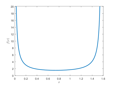
0φi(t)𝑑t=τf(λiτ)wheref(x)=12xcos(x)1sin(x),formulae-sequencesuperscriptsubscript0subscript𝜑𝑖𝑡differential-d𝑡𝜏𝑓subscript𝜆𝑖𝜏where𝑓𝑥12𝑥𝑥1𝑥\int_{0}^{\infty}\varphi_{i}(t)\,dt=\tau f(\lambda_{i}\tau)\leavevmode\nobreak\ \leavevmode\nobreak\ \text{where}\leavevmode\nobreak\ \leavevmode\nobreak\ f(x)=\frac{1}{2x}\frac{\cos(x)}{1-\sin(x)}, (10)

is a function defined in (0,π2)0𝜋2(0,\frac{\pi}{2}) that takes values in +subscript\mathbb{R}_{+}. The plot of f𝑓f is provided in Figure 1. The rigorous derivation of formula (10) is held in Appendix A. Delay Differential Equations.
Refer to caption
Figure 1: Plot of f(x)=12xcos(x)1sin(x)𝑓𝑥12𝑥𝑥1𝑥f(x)=\frac{1}{2x}\frac{\cos(x)}{1-\sin(x)} over its domain (0,π2)0𝜋2(0,\frac{\pi}{2}) that guarantees internal stability of network (6).

4.2 The Statistics of the Solution

The solution of the perturbed network (6) is an {t}t0subscriptsubscript𝑡𝑡0\{\mathcal{F}_{t}\}_{t\geq 0}-measurable stochastic process {𝐱t}tτsubscriptsubscript𝐱𝑡𝑡𝜏\{\mathbf{x}_{t}\}_{t\geq-\tau} given by

𝐱t=𝐯t+0tΦL(ts)B𝑑𝐰ssubscript𝐱𝑡subscript𝐯𝑡superscriptsubscript0𝑡subscriptΦ𝐿𝑡𝑠𝐵differential-dsubscript𝐰𝑠\mathbf{x}_{t}=\mathbf{v}_{t}+\int_{0}^{t}\Phi_{L}(t-s)B\,d\mathbf{w}_{s}

in which

𝐯t=ΦL(t)ϕ(0)Lτ0ΦL(tsτ)ϕ(s)𝑑s.subscript𝐯𝑡subscriptΦ𝐿𝑡bold-italic-ϕ0𝐿superscriptsubscript𝜏0subscriptΦ𝐿𝑡𝑠𝜏bold-italic-ϕ𝑠differential-d𝑠\mathbf{v}_{t}=\Phi_{L}(t)\boldsymbol{\phi}(0)-L\int_{-\tau}^{0}\Phi_{L}(t-s-\tau)\boldsymbol{\phi}(s)\,ds.

Moreover, it follows that 𝐱t𝒩(𝝁t,Σt)similar-tosubscript𝐱𝑡𝒩subscript𝝁𝑡subscriptΣ𝑡\mathbf{x}_{t}\sim\mathcal{N}(\boldsymbol{\mu}_{t},\Sigma_{t}) with vector-valued mean 𝝁t=𝔼[𝐯t]subscript𝝁𝑡𝔼delimited-[]subscript𝐯𝑡\boldsymbol{\mu}_{t}=\mathbb{E}\big{[}\mathbf{v}_{t}\big{]} and covariance matrix

Σt=b20tΦL(s)ΦLT(s)𝑑s.subscriptΣ𝑡superscript𝑏2superscriptsubscript0𝑡subscriptΦ𝐿𝑠superscriptsubscriptΦ𝐿𝑇𝑠differential-d𝑠\Sigma_{t}=b^{2}\int_{0}^{t}\Phi_{L}(s)\Phi_{L}^{T}(s)\,ds. (11)

4.3 The Statistics of the Output

Consequently, the statistics of the output can be quantified as

𝐲t𝒩(C𝝁t,CΣtCT).similar-tosubscript𝐲𝑡𝒩𝐶subscript𝝁𝑡𝐶subscriptΣ𝑡superscript𝐶𝑇\mathbf{y}_{t}\sim\mathcal{N}(C\boldsymbol{\mu}_{t},C\Sigma_{t}C^{T}). (12)

The following result characterizes output matrices for which 𝐲t𝕃2(q),t0formulae-sequencesubscript𝐲𝑡superscript𝕃2superscript𝑞𝑡0\mathbf{y}_{t}\in\mathbb{L}^{2}(\mathbb{R}^{q}),\leavevmode\nobreak\ t\geq 0.

Lemma 1.

𝟏nker(C)subscript1𝑛kernel𝐶\mathbf{1}_{n}\in\ker(C) if and only if

supt0CΣtCT<.subscriptsupremum𝑡0norm𝐶subscriptΣ𝑡superscript𝐶𝑇\sup_{t\geq 0}\leavevmode\nobreak\ \big{\|}C\Sigma_{t}C^{T}\big{\|}<\infty.

The result of Lemma 1 implies that if C𝐪1=0𝐶subscript𝐪10C\mathbf{q}_{1}=0, then one gets 𝐲¯=limt𝐲t𝕃2(q)¯𝐲subscript𝑡subscript𝐲𝑡superscript𝕃2superscript𝑞\overline{\mathbf{y}}=\lim_{t\rightarrow\infty}\mathbf{y}_{t}\in\mathbb{L}^{2}(\mathbb{R}^{q}) as both Σ¯=limtCΣtCT¯Σsubscript𝑡𝐶subscriptΣ𝑡superscript𝐶𝑇\overline{\Sigma}=\lim_{t\rightarrow\infty}C\Sigma_{t}C^{T} and 𝝁¯=limtC𝝁t¯𝝁subscript𝑡𝐶subscript𝝁𝑡\overline{\boldsymbol{\mu}}=\lim_{t\rightarrow\infty}C\boldsymbol{\mu}_{t} are well-defined. Moreover, 𝐲¯𝒩(0,Σ¯)similar-to¯𝐲𝒩0¯Σ\overline{\mathbf{y}}\sim\mathcal{N}(0,\overline{\Sigma}) if and only if 𝟏nker(C)subscript1𝑛kernel𝐶\mathbf{1}_{n}\in\ker(C).

5 Systemic Risk Measures

There are several known quantifiers in the context of finance and economy to measure risk of a systemic event. In this paper, we utilize two notions of risk measures, which are relevant to the context of dynamical systems, to quantify safety margins of network (6) before it experiences systemic event (9) and reaches a δ𝛿\delta-consensus based on Definitions 1 and 2.

5.1 Risk of Large Fluctuations in Probability

When network observables admit a well defined probability measure, we may be able to calculate risk of a systemic event that is expressed in terms of violation of a set of critical constraints; for example, stochastic event (9) in the rendezvous example. The value-at-risk measure, also referred to as risk in probability, determines maximum allowable fluctuation, which we also refer to it as safety margin, before network experiences a systemic event with a pre-specified probability. In other words, this measure quantifies the smallest lower bound δ𝛿\delta for systemic event z(ω)𝕃2()𝑧𝜔superscript𝕃2z(\omega)\in\mathbb{L}^{2}(\mathbb{R}) before probability of event “z(ω)𝑧𝜔z(\omega) surpassing δ𝛿\delta” exceeds a given threshold.

Definition 3.

For a given probability threshold ε[0,1)𝜀01\varepsilon\in[0,1), the value-at-risk or risk in probability is an operator ε:𝕃2():subscript𝜀superscript𝕃2\mathcal{R}_{\varepsilon}:\mathbb{L}^{2}(\mathbb{R})\rightarrow\mathbb{R} that is defined by

ε(z)=inf{δ|(z(ω)>δ)<ε}.subscript𝜀𝑧infimumconditional-set𝛿𝑧𝜔𝛿𝜀\mathcal{R}_{\varepsilon}(z)=\inf\Big{\{}\delta\in\mathbb{R}\leavevmode\nobreak\ \Big{|}\leavevmode\nobreak\ \mathbb{P}\big{(}z(\omega)>\delta\big{)}<\varepsilon\Big{\}}.

If the right hand-side has no solution, we set ε(z)=+subscript𝜀𝑧\mathcal{R}_{\varepsilon}(z)=+\infty.

The value-at-risk measure enjoys several functional properties that will help us later on to derive fundamental limits on the best achievable risk value and tradeoffs between risk and network connectivity.

Proposition 1.

The measure ε:𝕃2():subscript𝜀superscript𝕃2\mathcal{R}_{\varepsilon}:\mathbb{L}^{2}(\mathbb{R})\rightarrow\mathbb{R} in Definition 3 satisfies the properties:

  • (i)

    ε(z)=zsubscript𝜀𝑧𝑧\mathcal{R}_{\varepsilon}(z)=z if z𝑧z is independent of ωΩ𝜔Ω\omega\in\Omega.

  • (ii)

    ε(z+m)=ε(z)+msubscript𝜀𝑧𝑚subscript𝜀𝑧𝑚\mathcal{R}_{\varepsilon}(z+m)=\mathcal{R}_{\varepsilon}(z)+m for all m𝑚m\in\mathbb{R}.

  • (iii)

    If z1z2subscript𝑧1subscript𝑧2z_{1}\leq z_{2}, then ε(z1)ε(z2)subscript𝜀subscript𝑧1subscript𝜀subscript𝑧2\mathcal{R}_{\varepsilon}(z_{1})\leq\mathcal{R}_{\varepsilon}(z_{2})

  • (iv)

    ε(αz)=αε(z)subscript𝜀𝛼𝑧𝛼subscript𝜀𝑧\mathcal{R}_{\varepsilon}(\alpha z)=\alpha\mathcal{R}_{\varepsilon}(z) for α>0𝛼0\alpha>0.

  • (v)

    ε(z)subscript𝜀𝑧\mathcal{R}_{\varepsilon}(z) is a quasi-convex function of z𝑧z.

Property (i) implies that if a z𝑧z includes no uncertainty, the risk measure remains invariant. Property (ii) means that εsubscript𝜀\mathcal{R}_{\varepsilon} is not affected when a fixed constant is added to the random variable. Property (iii) explains that if a random variable z1subscript𝑧1z_{1} takes smaller values than z2subscript𝑧2z_{2} almost surely, then the risk of the former is smaller than the risk of the latter. Next, (iv) is a positive homogeneity property and implies that if we scale a random variable (i.e., scale the uncertainty with it) then the risk will scale accordingly. Finally, property (v) is a weak convexity property of the risk measure and indicates that the risk of a convex combination of two random variables cannot get worse than the maximum of the risk of these random variables.

5.2 Risk of Large Fluctuations in Expectation

The second type of risk measures that are relevant to the context of dynamical systems is quantification of risk through statistical expectation of a utility or cost function. In several applications in economics, game theory, and decision and control theory, we evaluate violation of critical constraints against some meaningful utility or cost functions. These utility functions reflect perception of a decision maker towards a potential outcome when there is uncertainty [10]. In this setting, utility function can be interpreted as a distance function to measure how far a random variable is from a predefined threshold. This interpretation is particularly useful in the context of dynamical systems as one can employ energy or entropy based utility functions to quantify risk.

Definition 4.

Suppose that utility function v::𝑣v:{\mathbb{R}}\rightarrow{\mathbb{R}} is convex and monotonically increasing. For a given threshold ε𝜀\varepsilon, the risk in expectation is an operator 𝒯ε:𝕃2():subscript𝒯𝜀superscript𝕃2\mathcal{T}_{\varepsilon}:\mathbb{L}^{2}(\mathbb{R})\rightarrow\mathbb{R} that is defined by

𝒯ε(z)=inf{δ|𝔼[v(z(ω)δ)]<v(ε)}.subscript𝒯𝜀𝑧infimumconditional-set𝛿𝔼delimited-[]𝑣𝑧𝜔𝛿𝑣𝜀\mathcal{T}_{\varepsilon}(z)=\inf\Big{\{}\delta\in\mathbb{R}\leavevmode\nobreak\ \Big{|}\leavevmode\nobreak\ \mathbb{E}\big{[}v\big{(}z(\omega)-\delta\big{)}\big{]}<v(\varepsilon)\Big{\}}.

If the right hand-side has no solution, we set 𝒯ε(z)=+subscript𝒯𝜀𝑧\mathcal{T}_{\varepsilon}(z)=+\infty.

The risk in expectation quantifies possibility of large fluctuations by evaluating expected value of a predefined utility or cost function. A trivial choice for utility function is v(z)=z𝑣𝑧𝑧v(z)=z, where the value of risk is the smallest number for which inequality 𝔼[z(ω)δ]ε𝔼delimited-[]𝑧𝜔𝛿𝜀\mathbb{E}[z(\omega)-\delta]\leq\varepsilon holds. For more general utility functions, we can still relate to this simple inequality by applying Jensen’s inequality and monotonicity property of the utility function. It is straightforward to show that 𝒯εsubscript𝒯𝜀\mathcal{T}_{\varepsilon} is positive if and only if 𝔼[v(z)]>v(ε)𝔼delimited-[]𝑣𝑧𝑣𝜀\mathbb{E}\big{[}v(z)\big{]}>v(\varepsilon) (we refer to [10] for more details). This helps us to define the following acceptance set

𝔸={z𝕃2()|𝒯ε(z)<0}𝔸conditional-set𝑧superscript𝕃2subscript𝒯𝜀𝑧0\mathbb{A}=\Big{\{}\leavevmode\nobreak\ z\in\mathbb{L}^{2}(\mathbb{R})\leavevmode\nobreak\ \Big{|}\leavevmode\nobreak\ \mathcal{T}_{\varepsilon}(z)<0\leavevmode\nobreak\ \Big{\}} (13)

that contains all random variables in 𝕃2()superscript𝕃2\mathbb{L}^{2}(\mathbb{R}) whose expected cost 𝔼[v(z)]𝔼delimited-[]𝑣𝑧\mathbb{E}[v(z)] is less than cost threshold v(ε)𝑣𝜀v(\varepsilon). In the following, we discuss two important and relevant utility functions for risk analysis in dynamical systems.

Quadratic Utility: For scalar random variables, the quadratic utility function is v(z)=z2𝑣𝑧superscript𝑧2v(z)=z^{2} over nonnegative real numbers. The value of risk in this case represents the smallest value δ𝛿\delta for which random variable z𝑧z stays in a ball with center δ𝛿\delta and radius v(ε)𝑣𝜀v(\varepsilon). Depending on the application, quadratic form of the output (7) relates to the potential or kinetic energies of the system [37].

Exponential Utility: For scalar random variables, the exponential utility function is v(z)=eβz𝑣𝑧superscript𝑒𝛽𝑧v(z)=e^{\beta z} for some parameter β>0𝛽0\beta>0. This function is monotonically increasing over all real numbers and close in spirit to the entropic risk measure [10].

Proposition 2.

The risk in expectation 𝒯ε:𝕃2():subscript𝒯𝜀superscript𝕃2\mathcal{T}_{\varepsilon}:\mathbb{L}^{2}(\mathbb{R})\rightarrow\mathbb{R} as in Definition 4 satisfies the following properties:

  • (i)

    𝒯ε(z+m)=Tε(z)+msubscript𝒯𝜀𝑧𝑚subscript𝑇𝜀𝑧𝑚\mathcal{T}_{\varepsilon}(z+m)=T_{\varepsilon}(z)+m for all m𝑚m\in\mathbb{R}.

  • (ii)

    𝒯ε(z)subscript𝒯𝜀𝑧\mathcal{T}_{\varepsilon}(z) is a convex function of z𝔸𝑧𝔸z\in\mathbb{A}.

  • (iii)

    z1z2subscript𝑧1subscript𝑧2z_{1}\leq z_{2} implies 𝒯ε(z1)𝒯ε(z2)subscript𝒯𝜀subscript𝑧1subscript𝒯𝜀subscript𝑧2\mathcal{T}_{\varepsilon}(z_{1})\leq\mathcal{T}_{\varepsilon}(z_{2}).

  • (iv)

    For all nonnegative z𝔸𝑧𝔸z\in\mathbb{A}, it follows that

    𝒯ε(αz)α𝒯ε(z)+(α1)εsubscript𝒯𝜀𝛼𝑧𝛼subscript𝒯𝜀𝑧𝛼1𝜀\mathcal{T}_{\varepsilon}(\alpha z)\geq\alpha\mathcal{T}_{\varepsilon}(z)+(\alpha-1)\varepsilon

    for all α1𝛼1\alpha\geq 1, and for all nonpositive z𝔸𝑧𝔸z\in\mathbb{A}, we have

    𝒯ε(αz)α𝒯ε(z)(α1)εsubscript𝒯𝜀𝛼𝑧𝛼subscript𝒯𝜀𝑧𝛼1𝜀\mathcal{T}_{\varepsilon}(\alpha z)\leq\mathcal{\alpha}\mathcal{T}_{\varepsilon}(z)-(\alpha-1)\varepsilon

    for all α[0,1]𝛼01\alpha\in[0,1].

Property (i) is the equivalent of Property (ii) in Proposition 1. It explains that adding fixed numbers (with no uncertainty) does not affect the value of risk in expectation. The convexity property of Property (ii) holds within the acceptance set (13) and can be generalized to any acceptance set that is convex [10]. Property (iii) means that risk in expectation is monotonically increasing. According to property (iv), the risk measure enjoys a weak positive homogeneity property that holds over a subset of 𝔸𝔸\mathbb{A}.

6 Risk Assessment of a Single Event

Suppose that the network observable is scalar

yt=𝐜T𝐱tsubscript𝑦𝑡superscript𝐜𝑇subscript𝐱𝑡y_{t}=\mathbf{c}^{T}\mathbf{x}_{t} (14)

with 𝐜n𝐜superscript𝑛\mathbf{c}\in{\mathbb{R}}^{n}. According to (12), it follows that yt𝒩(μt,σt2)similar-tosubscript𝑦𝑡𝒩subscript𝜇𝑡superscriptsubscript𝜎𝑡2y_{t}\sim\mathcal{N}(\mu_{t},\sigma_{t}^{2}) with

μtsubscript𝜇𝑡\displaystyle\mu_{t} =\displaystyle= 𝔼[k=1nckQ[φk(t)ϕkQ(0)+τ0φk(t+s)ϕkQ(s)𝑑s]]𝔼delimited-[]superscriptsubscript𝑘1𝑛superscriptsubscript𝑐𝑘𝑄delimited-[]subscript𝜑𝑘𝑡superscriptsubscriptitalic-ϕ𝑘𝑄0superscriptsubscript𝜏0subscript𝜑𝑘𝑡𝑠superscriptsubscriptitalic-ϕ𝑘𝑄𝑠differential-d𝑠\displaystyle\mathbb{E}\bigg{[}\sum_{k=1}^{n}c_{k}^{Q}\big{[}\varphi_{k}(t)\phi_{k}^{Q}(0)+\int_{-\tau}^{0}\varphi_{k}(t+s)\phi_{k}^{Q}(s)\,ds\big{]}\bigg{]} (15)
σt2superscriptsubscript𝜎𝑡2\displaystyle\sigma_{t}^{2} =\displaystyle= b2k=1n(ckQ)20tφk2(s)𝑑s,superscript𝑏2superscriptsubscript𝑘1𝑛superscriptsuperscriptsubscript𝑐𝑘𝑄2superscriptsubscript0𝑡superscriptsubscript𝜑𝑘2𝑠differential-d𝑠\displaystyle b^{2}\sum_{k=1}^{n}(c_{k}^{Q})^{2}\int_{0}^{t}\varphi_{k}^{2}(s)\,ds, (16)

where 𝐜Q=[c1Q,,ckQ]Tsuperscript𝐜𝑄superscriptsuperscriptsubscript𝑐1𝑄superscriptsubscript𝑐𝑘𝑄𝑇\mathbf{c}^{Q}=[c_{1}^{Q},\dots,c_{k}^{Q}]^{T} and ϕQ(t)=[ϕ1Q,,ϕkQ]T,t[τ,0]formulae-sequencesuperscriptbold-italic-ϕ𝑄𝑡superscriptsuperscriptsubscriptitalic-ϕ1𝑄superscriptsubscriptitalic-ϕ𝑘𝑄𝑇𝑡𝜏0\boldsymbol{\phi}^{Q}(t)=[\phi_{1}^{Q},\dots,\phi_{k}^{Q}]^{T},t\in[-\tau,0] are the corresponding vectors 𝐜𝐜\mathbf{c} and ϕ(t)bold-italic-ϕ𝑡\boldsymbol{\phi}(t) represented in terms of the basis spanned by the columns of Q=[𝐪1||𝐪n]𝑄delimited-[]subscript𝐪1subscript𝐪𝑛Q=[\mathbf{q}_{1}\hskip 1.42271pt|\hskip 1.42271pt\dots\hskip 1.42271pt|\hskip 1.42271pt\mathbf{q}_{n}], for 𝐪ksubscript𝐪𝑘\mathbf{q}_{k} is the k𝑘k’th Laplacian eigenvector, and {φk}k𝒱subscriptsubscript𝜑𝑘𝑘𝒱\{\varphi_{k}\}_{k\in{\mathcal{V}}} the diagonal elements of principal matrix ΦΦ\Phi.

Lemma 2.

For every time instant t𝑡t, functions μt=μt(Q)subscript𝜇𝑡subscript𝜇𝑡𝑄\mu_{t}=\mu_{t}(Q) and σt=σ2(Q)subscript𝜎𝑡subscript𝜎2𝑄\sigma_{t}=\sigma_{2}(Q), as they are defined by (15) and (16), are eigenspace invariant, i.e., for all orthonormal matrices Q1subscript𝑄1Q_{1} and Q2subscript𝑄2Q_{2} for which Q1ΛQ1T=Q2ΛQ2Tsubscript𝑄1Λsuperscriptsubscript𝑄1𝑇subscript𝑄2Λsuperscriptsubscript𝑄2𝑇Q_{1}\Lambda Q_{1}^{T}=Q_{2}\Lambda Q_{2}^{T}, we have

μt(Q1)=μt(Q2)andσt(Q1)=σt(Q2).formulae-sequencesubscript𝜇𝑡subscript𝑄1subscript𝜇𝑡subscript𝑄2andsubscript𝜎𝑡subscript𝑄1subscript𝜎𝑡subscript𝑄2\mu_{t}(Q_{1})=\mu_{t}(Q_{2})\leavevmode\nobreak\ \leavevmode\nobreak\ \leavevmode\nobreak\ \textrm{and}\leavevmode\nobreak\ \leavevmode\nobreak\ \leavevmode\nobreak\ \sigma_{t}(Q_{1})=\sigma_{t}(Q_{2}).
Theorem 1.

Suppose that stochastic process 𝐱={𝐱t}t[τ,T]𝐱subscriptsubscript𝐱𝑡𝑡𝜏𝑇\mathbf{x}=\{\mathbf{x}_{t}\}_{t\in[-\tau,T]} is the solution of (6) and the network observable is scalar as in (14). Then, the risk of large fluctuations in probability is given by

ε(|yt|)=2σtSε(μt2σt)+μt,subscript𝜀subscript𝑦𝑡2subscript𝜎𝑡subscript𝑆𝜀subscript𝜇𝑡2subscript𝜎𝑡subscript𝜇𝑡\mathcal{R}_{\varepsilon}(|y_{t}|)=\sqrt{2}\sigma_{t}S_{\varepsilon}\bigg{(}\frac{\mu_{t}}{\sqrt{2}\sigma_{t}}\bigg{)}+\mu_{t}, (17)

where Sε()subscript𝑆𝜀S_{\varepsilon}(\cdot) is defined by (3), and the risk of output fluctuations violating a utility threshold can be calculated as follows:

(i) when u(z)=z2𝑢𝑧superscript𝑧2u(z)=z^{2},

𝒯ε(|yt|)={μ|yt|ε2σ|yt|2ifεσ|yt|+otherwisesubscript𝒯𝜀subscript𝑦𝑡casessubscript𝜇subscript𝑦𝑡superscript𝜀2superscriptsubscript𝜎subscript𝑦𝑡2if𝜀subscript𝜎subscript𝑦𝑡otherwise\mathcal{T}_{\varepsilon}(|y_{t}|)=\begin{cases}\mu_{|y_{t}|}-\sqrt{\varepsilon^{2}-\sigma_{|y_{t}|}^{2}}&\textrm{if}\leavevmode\nobreak\ \leavevmode\nobreak\ \leavevmode\nobreak\ \varepsilon\geq\sigma_{|y_{t}|}\\ +\infty&\textrm{otherwise}\end{cases} (18)

(ii) when u(z)=eβz𝑢𝑧superscript𝑒𝛽𝑧u(z)=e^{\beta z} for some β>0𝛽0\beta>0,

𝒯ε(|yt|)=βσt22+ln(κ(μt,σt)/2)βεsubscript𝒯𝜀subscript𝑦𝑡𝛽superscriptsubscript𝜎𝑡22𝜅subscript𝜇𝑡subscript𝜎𝑡2𝛽𝜀\begin{split}\mathcal{T}_{\varepsilon}(|y_{t}|)=\frac{\beta\sigma_{t}^{2}}{2}&+\frac{\ln\big{(}\kappa(\mu_{t},\sigma_{t})/2\big{)}}{\beta}-\varepsilon\end{split} (19)

in which

μ|yt|subscript𝜇subscript𝑦𝑡\displaystyle\mu_{|y_{t}|} =\displaystyle= σt2πeμt22σt2μterf(μt2σt2)subscript𝜎𝑡2𝜋superscript𝑒superscriptsubscript𝜇𝑡22superscriptsubscript𝜎𝑡2subscript𝜇𝑡erfsubscript𝜇𝑡2superscriptsubscript𝜎𝑡2\displaystyle\sigma_{t}\sqrt{\frac{2}{\pi}}e^{-\frac{\mu_{t}^{2}}{2\sigma_{t}^{2}}}-\mu_{t}\leavevmode\nobreak\ \mathrm{erf}\bigg{(}\frac{-\mu_{t}}{\sqrt{2\sigma_{t}^{2}}}\bigg{)}
σ|yt|2superscriptsubscript𝜎subscript𝑦𝑡2\displaystyle\sigma_{|y_{t}|}^{2} =\displaystyle= μt2+σt2μ|yt|2,superscriptsubscript𝜇𝑡2superscriptsubscript𝜎𝑡2superscriptsubscript𝜇subscript𝑦𝑡2\displaystyle\mu_{t}^{2}+\sigma_{t}^{2}-\mu_{|y_{t}|}^{2},
κ(μt,σt)𝜅subscript𝜇𝑡subscript𝜎𝑡\displaystyle\kappa(\mu_{t},\sigma_{t}) =\displaystyle= [1erf(μt2σtβσt2)]eβμtdelimited-[]1erfsubscript𝜇𝑡2subscript𝜎𝑡𝛽subscript𝜎𝑡2superscript𝑒𝛽subscript𝜇𝑡\displaystyle\bigg{[}1-\mathrm{erf}\bigg{(}-\frac{\mu_{t}}{\sqrt{2}\sigma_{t}}-\frac{\beta\sigma_{t}}{\sqrt{2}}\bigg{)}\bigg{]}e^{\beta\mu_{t}}
+[1+erf(μt2σt+βσt2)]eβμtdelimited-[]1erfsubscript𝜇𝑡2subscript𝜎𝑡𝛽subscript𝜎𝑡2superscript𝑒𝛽subscript𝜇𝑡\displaystyle+\bigg{[}1+\mathrm{erf}\bigg{(}-\frac{\mu_{t}}{\sqrt{2}\sigma_{t}}+\frac{\beta\sigma_{t}}{\sqrt{2}}\bigg{)}\bigg{]}e^{-\beta\mu_{t}}

and μtsubscript𝜇𝑡\mu_{t} and σtsubscript𝜎𝑡\sigma_{t} are defined by (15)-(16).

In case of no time delay, i.e., τ=0𝜏0\tau=0, the eigensolutions of the nominal system take simple forms φk(t)=eλktsubscript𝜑𝑘𝑡superscript𝑒subscript𝜆𝑘𝑡\varphi_{k}(t)=e^{-\lambda_{k}t} for k=2,,n𝑘2𝑛k=2,\ldots,n. This allows us to derive a more explicit form for the variance:

σt2=b2k=2n(ckQ)21e2λkt2λk.superscriptsubscript𝜎𝑡2superscript𝑏2superscriptsubscript𝑘2𝑛superscriptsuperscriptsubscript𝑐𝑘𝑄21superscript𝑒2subscript𝜆𝑘𝑡2subscript𝜆𝑘\sigma_{t}^{2}=b^{2}\sum_{k=2}^{n}\leavevmode\nobreak\ (c_{k}^{Q})^{2}\leavevmode\nobreak\ \frac{1-e^{-2\lambda_{k}t}}{2\lambda_{k}}.

When τ>0𝜏0\tau>0 and t<𝑡t<\infty, the risk expressions in Theorem 1 do not admit more tractable representations in general. However, towards the end of this section, we show that in steady state (as t𝑡t\rightarrow\infty) one can obtain more explicit formulas for systemic risk measures; we also refer to [41] for more details.

The steady state behavior of systemic risk measures can be investigated by letting t𝑡t tend to infinity. According to Lemma 1, if output matrix C𝐶C is orthogonal to the vector of all ones, then y¯=limtyt¯𝑦subscript𝑡subscript𝑦𝑡\overline{y}=\lim_{t\rightarrow\infty}y_{t} will belong to 𝕃2()superscript𝕃2\mathbb{L}^{2}(\mathbb{R}), i.e. with finite variance, denoted as σ¯¯𝜎\overline{\sigma}. If 𝐜T𝟙n=0superscript𝐜𝑇subscript1𝑛0\mathbf{c}^{T}\mathbbm{1}_{n}=0, then μtsubscript𝜇𝑡\mu_{t} vanishes exponentially fast. In steady state, the transient effect of initial conditions disappears and other origins of large volatility and fluctuation in network observables reveal themselves, e.g., communication topology, time delay, and the diffusion coefficient b𝑏b. The steady-state risk analysis uncovers how exogenous noise propagates throughout the network, is amplified by various factors, and results in rapid and unpredictable variations in network observables.

Theorem 2.

Suppose that stochastic process 𝐱={𝐱t}tτ𝐱subscriptsubscript𝐱𝑡𝑡𝜏\mathbf{x}=\{\mathbf{x}_{t}\}_{t\geq-\tau} is the solution of (6) and the network observable is scalar as in (14) and the output matrix satisfies 𝐜T𝟙n=0superscript𝐜𝑇subscript1𝑛0\mathbf{c}^{T}\mathbbm{1}_{n}=0. Then, the risk of large fluctuations in probability in steady-state is given by

ε(|y¯|)=2Sε(0)σ¯subscript𝜀¯𝑦2subscript𝑆𝜀0¯𝜎\mathcal{R}_{\varepsilon}(|\overline{y}|)=\sqrt{2}\hskip 1.42271ptS_{\varepsilon}(0)\hskip 1.42271pt\overline{\sigma} (20)

in which

σ¯2=12b2k=2ncos(λkτ)λk(1sin(λkτ))(ckQ)2superscript¯𝜎212superscript𝑏2superscriptsubscript𝑘2𝑛subscript𝜆𝑘𝜏subscript𝜆𝑘1subscript𝜆𝑘𝜏superscriptsuperscriptsubscript𝑐𝑘𝑄2\overline{\sigma}^{2}\hskip 1.42271pt=\hskip 1.42271pt\frac{1}{2}\hskip 1.42271ptb^{2}\hskip 1.42271pt\sum_{k=2}^{n}\hskip 1.42271pt\frac{\cos(\lambda_{k}\tau)}{\lambda_{k}\big{(}1-\sin(\lambda_{k}\tau)\big{)}}\hskip 1.42271pt(c_{k}^{Q})^{2} (21)

where λksubscript𝜆𝑘\lambda_{k} is the k𝑘k’th non-zero Laplacian eigenvalue. The risk of output fluctuations violating a utility threshold in steady-state w.r.t.:

(i) quadratic utility v(x)=x2𝑣𝑥superscript𝑥2v(x)=x^{2} is given by

𝒯ε(|y¯|)={2πσ¯ε2(12π)σ¯2ifεσ¯12π+otherwisesubscript𝒯𝜀¯𝑦cases2𝜋¯𝜎superscript𝜀212𝜋superscript¯𝜎2if𝜀¯𝜎12𝜋otherwise\mathcal{T}_{\varepsilon}(|\overline{y}|)=\begin{cases}\sqrt{\frac{2}{\pi}}\overline{\sigma}-\sqrt{\varepsilon^{2}-\big{(}1-\frac{2}{\pi}\big{)}\overline{\sigma}^{2}}&\textrm{if}\leavevmode\nobreak\ \leavevmode\nobreak\ \varepsilon\geq\overline{\sigma}\sqrt{1-\frac{2}{\pi}}\\ +\infty&\text{otherwise}\end{cases} (22)

(ii) exponential utility v(x)=eβx𝑣𝑥superscript𝑒𝛽𝑥v(x)=e^{\beta x} for some β>0𝛽0\beta>0 can be expressed by

𝒯ε(|y¯|)=βσ¯22+ln(1+erf(βσ¯2))βε.subscript𝒯𝜀¯𝑦𝛽superscript¯𝜎221erf𝛽¯𝜎2𝛽𝜀\begin{split}\mathcal{T}_{\varepsilon}(|\overline{y}|)=\frac{\beta\overline{\sigma}^{2}}{2}&+\frac{\ln\big{(}1+\mathrm{erf}(\frac{\beta\overline{\sigma}}{2})\big{)}}{\beta}-\varepsilon.\end{split} (23)

The expression for variance (21) can be equivalently written in the following compact form444The Moore-Penrose pseudo-inverse of matrix L𝐿L is denoted by Lsuperscript𝐿L^{\dagger}. For a matrix Xn×n𝑋superscript𝑛𝑛X\in\mathbb{R}^{n\times n}, the matrix-valued functions of matrices cos(X)𝑋\cos(X) and sin(X)𝑋\sin(X) are defined as cos(X)=k=0(1)k(2k)!X2k𝑋superscriptsubscript𝑘0superscript1𝑘2𝑘superscript𝑋2𝑘\cos(X)=\sum_{k=0}^{\infty}\frac{(-1)^{k}}{(2k)!}X^{2k} and sin(X)=k=0(1)k(2k+1)!X2k+1𝑋superscriptsubscript𝑘0superscript1𝑘2𝑘1superscript𝑋2𝑘1\sin(X)=\sum_{k=0}^{\infty}\frac{(-1)^{k}}{(2k+1)!}X^{2k+1}.

σ¯2=12b2Tr[LoLcos(τL)(Mnsin(τL))]superscript¯𝜎212superscript𝑏2Trdelimited-[]subscript𝐿𝑜superscript𝐿𝜏𝐿superscriptsubscript𝑀𝑛𝜏𝐿\overline{\sigma}^{2}\hskip 1.42271pt=\hskip 1.42271pt\frac{1}{2}\hskip 1.42271ptb^{2}\hskip 1.42271pt\mathrm{Tr}\Big{[}L_{o}\hskip 1.42271ptL^{\dagger}\cos(\tau L)\big{(}M_{n}-\sin(\tau L)\big{)}^{\dagger}\Big{]} (24)

where Lo=𝐜𝐜Tsubscript𝐿𝑜superscript𝐜𝐜𝑇L_{o}=\mathbf{c}\mathbf{c}^{T}. In the following, we discuss some of the important and useful examples of scalar network observables.

(a) Deviation of a single state from the average: Suppose that we are interested in observing state of agent i𝑖i. The deviation from average of xisubscript𝑥𝑖x_{i} can be obtained by choosing the i𝑖i’th column of the centering matrix Mnsubscript𝑀𝑛M_{n} as the output matrix, i.e., 𝐜=𝐦i𝐜subscript𝐦𝑖\mathbf{c}=\mathbf{m}_{i}. A direction calculation reveals that

ckQ={0ifk=1𝐦iT𝐪kifk=2,,n.superscriptsubscript𝑐𝑘𝑄cases0if𝑘1superscriptsubscript𝐦𝑖𝑇subscript𝐪𝑘if𝑘2𝑛c_{k}^{Q}=\left\{\begin{array}[]{ccc}0&\textrm{if}&k=1\\ \mathbf{m}_{i}^{T}\mathbf{q}_{k}&\textrm{if}&k=2,\ldots,n\end{array}\right..

(b) Pairwise deviation: When one is interested in characterizing volatility of the disagreement between two specific fixed agents, say agents with labels i𝑖i and j𝑗j, we choose output matrix 𝐜=𝐞i𝐞j𝐜subscript𝐞𝑖subscript𝐞𝑗\mathbf{c}=\mathbf{e}_{i}-\mathbf{e}_{j}. In this case,

ckQ={0ifk=1(𝐞i𝐞j)T𝐪kifk=2,,n.superscriptsubscript𝑐𝑘𝑄cases0if𝑘1superscriptsubscript𝐞𝑖subscript𝐞𝑗𝑇subscript𝐪𝑘if𝑘2𝑛c_{k}^{Q}=\left\{\begin{array}[]{ccc}0&\textrm{if}&k=1\\ (\mathbf{e}_{i}-\mathbf{e}_{j})^{T}\mathbf{q}_{k}&\textrm{if}&k=2,\ldots,n\end{array}\right..

(c) Deviation from average of immediate neighbors: Comparing state of each agent with average of its own adjacent neighbors is another meaningful observable for network (6). In this case, the components of the output matrix are defined as

ckQ={0ifk=1𝐪kT(𝐞i1niji𝐞j)ifk=2,,n,superscriptsubscript𝑐𝑘𝑄cases0if𝑘1superscriptsubscript𝐪𝑘𝑇subscript𝐞𝑖1subscript𝑛𝑖subscriptsimilar-to𝑗𝑖subscript𝐞𝑗if𝑘2𝑛c_{k}^{Q}=\left\{\begin{array}[]{ccc}0&\textrm{if}&k=1\\ \displaystyle\mathbf{q}_{k}^{T}\left(\mathbf{e}_{i}-\frac{1}{n_{i}}\sum_{j\sim i}\mathbf{e}_{j}\right)&\textrm{if}&k=2,\ldots,n\end{array}\right.,

where {j|ji}conditional-set𝑗similar-to𝑗𝑖\{j\hskip 1.42271pt|\hskip 1.42271ptj\sim i\} is equal to set {j|{i,j}}conditional-set𝑗𝑖𝑗\{j\hskip 1.42271pt|\hskip 1.42271pt\{i,j\}\in\mathcal{E}\} and nisubscript𝑛𝑖n_{i} is its cardinality.

In all these scenarios, the value of systemic risk measure 𝒯ε(|yt|)subscript𝒯𝜀subscript𝑦𝑡\mathcal{T}_{\varepsilon}(|y_{t}|) and ε(|yt|)subscript𝜀subscript𝑦𝑡\mathcal{R}_{\varepsilon}(|y_{t}|) can be calculated using Theorem 1 with statistical parameters defined in (15) and (16). Moreover, Theorem 2 shows that value of the systemic risk measure depend on Laplacian spectrum.

Remark 2.

When the output matrix is 𝐜=1n𝟙n𝐜1𝑛subscript1𝑛\mathbf{c}=\frac{1}{n}\mathbbm{1}_{n}, the network observable becomes the average of all states. It follows that c1Q=1nsuperscriptsubscript𝑐1𝑄1𝑛c_{1}^{Q}=\frac{1}{\sqrt{n}} and ckQ=0superscriptsubscript𝑐𝑘𝑄0c_{k}^{Q}=0 for every k>1𝑘1k>1. In this case, the mean and variance of the scalar observable reduces to

μt=1n[ϕ1Q(0)+τ0ϕ1Q(s)𝑑s]andσt2=b2n2t.formulae-sequencesubscript𝜇𝑡1𝑛delimited-[]superscriptsubscriptitalic-ϕ1𝑄0superscriptsubscript𝜏0superscriptsubscriptitalic-ϕ1𝑄𝑠differential-d𝑠andsuperscriptsubscript𝜎𝑡2superscript𝑏2superscript𝑛2𝑡\mu_{t}=\frac{1}{\sqrt{n}}\bigg{[}\phi_{1}^{Q}(0)+\int_{-\tau}^{0}\phi_{1}^{Q}(s)\,ds\bigg{]}\leavevmode\nobreak\ \leavevmode\nobreak\ \leavevmode\nobreak\ \textrm{and}\leavevmode\nobreak\ \leavevmode\nobreak\ \leavevmode\nobreak\ \sigma_{t}^{2}=\frac{b^{2}}{n^{2}}t. (25)

Using these formulas, one can compute the value of transient systemic risk measures 𝒯ε(|yt|)subscript𝒯𝜀subscript𝑦𝑡\mathcal{T}_{\varepsilon}(|y_{t}|) and ε(|yt|)subscript𝜀subscript𝑦𝑡\mathcal{R}_{\varepsilon}(|y_{t}|) according to Theorem 1. Since network (6) has a marginally stable mode corresponding to λ1=0subscript𝜆10\lambda_{1}=0, the variance σt2superscriptsubscript𝜎𝑡2\sigma_{t}^{2} diverges as t𝑡t grows (see also Lemma 1). This implies that all states fluctuate around their average and eventually diverge. This phenomenon is so-called “flocking to default” in finance and economy literature; we refer to [11, Ch. 17] for a discussion. Furthermore, one also observes that the stastistical parameters in (25) are independent of the network topology and time delay.

We conclude this section by investigating effects of time delay on systemic risk measures.

Theorem 3.

Suppose that the conditions of Theorem 2 are satisfied. Then, systemic risk measures (20), (22), (23) are strictly increasing functions of time delay.

Remark 3.

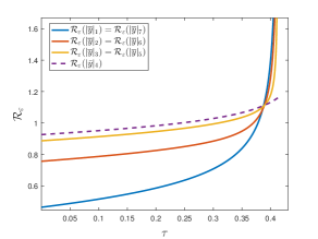
The class of systemic risk measures in this paper exhibit some idiosyncratic behavior in presence of time delay. It can be easily shown that the variance (21) is a convex function of eigenvalues. Systemic risks are in turn increasing functions of variance, which is not monotonically decreasing with respect to connectivity. This imposes counter-intuitive challenges in design of optimal networks with respect to this class of risk measures. For instance, increasing connectivity may deteriorate systemic risk of network (6) and sparsification may improve it. Figure 1 depicts behavior of each spectral term in expression of variance (21). The unorthodox behavior of risk and its interplay with connectivity and performance in time-delay networks is highly counterintuitive and requires careful investigations. In Section 9, we characterize an intrinsic tradeoff that explains this behavior.

7 Joint Risk Assessment of Multiple Events

The extension of risk for network (6) with vector valued output observables

𝐲t=C𝐱t=[𝐜1T𝐱t,,𝐜qT𝐱t]Tsubscript𝐲𝑡𝐶subscript𝐱𝑡superscriptsuperscriptsubscript𝐜1𝑇subscript𝐱𝑡superscriptsubscript𝐜𝑞𝑇subscript𝐱𝑡𝑇\mathbf{y}_{t}=C\mathbf{x}_{t}=\left[\hskip 1.42271pt\mathbf{c}_{1}^{T}\mathbf{x}_{t}\hskip 1.42271pt,\hskip 1.42271pt\ldots\hskip 1.42271pt,\hskip 1.42271pt\mathbf{c}_{q}^{T}\mathbf{x}_{t}\hskip 1.42271pt\right]^{T} (26)

is a problem with different approaches, each of which highlights the problem from a different perspective. In this section we introduce the most important multi-value risk measures for the steady state distribution of |𝐲t|=[|y1|,,|yq|]Tsubscript𝐲𝑡superscriptsubscript𝑦1subscript𝑦𝑞𝑇|\mathbf{y}_{t}|=\big{[}\hskip 1.42271pt|y_{1}|,\hskip 1.42271pt\dots\hskip 1.42271pt,|y_{q}|\hskip 1.42271pt\big{]}^{T} with yk=𝐜kT𝐱tsubscript𝑦𝑘superscriptsubscript𝐜𝑘𝑇subscript𝐱𝑡y_{k}=\mathbf{c}_{k}^{T}\mathbf{x}_{t}. We recall from Section 4 that in steady-state

𝐲¯𝒩(𝟎,Σ¯)similar-to¯𝐲𝒩0¯Σ\overline{\mathbf{y}}\sim\mathcal{N}({\mathbf{0}},\overline{\Sigma})

if and only if 𝟙nsubscript1𝑛\mathbbm{1}_{n} is in the kernel of output matrix C𝐶C.

When different types of observations are used for risk analysis in a dynamical network, systemic risk measure becomes a vector, where every element of that vector corresponds to the value of risk of an event that has a similar nature to the corresponding observation. For example, suppose that our goal is to evaluate risk using vector of observables 𝐲t=[y1(t),y2(t),y3(t)]Tsubscript𝐲𝑡superscriptsubscript𝑦1𝑡subscript𝑦2𝑡subscript𝑦3𝑡𝑇\mathbf{y}_{t}=[\hskip 1.42271pty_{1}(t),y_{2}(t),y_{3}(t)\hskip 1.42271pt]^{T}, where stochastic variable y1subscript𝑦1y_{1} measures deviation of a single state from the average of all states, y2subscript𝑦2y_{2} shows pairwise deviation between two given agents, and y3subscript𝑦3y_{3} gives deviation of a single state from average of its immediate neighbors.

8 Joint Risk Assessment of Multiple Events

The extension of risk for network (6) with vector valued output observables

𝐲t=C𝐱t=[𝐜1T𝐱t,,𝐜qT𝐱t]Tsubscript𝐲𝑡𝐶subscript𝐱𝑡superscriptsuperscriptsubscript𝐜1𝑇subscript𝐱𝑡superscriptsubscript𝐜𝑞𝑇subscript𝐱𝑡𝑇\mathbf{y}_{t}=C\mathbf{x}_{t}=\left[\hskip 1.42271pt\mathbf{c}_{1}^{T}\mathbf{x}_{t}\hskip 1.42271pt,\hskip 1.42271pt\ldots\hskip 1.42271pt,\hskip 1.42271pt\mathbf{c}_{q}^{T}\mathbf{x}_{t}\hskip 1.42271pt\right]^{T} (27)

is a problem with different approaches, each of which highlights the problem from a different perspective. In this section we introduce the most important multi-value risk measures for the steady state distribution of |𝐲t|=[|y1|,,|yq|]Tsubscript𝐲𝑡superscriptsubscript𝑦1subscript𝑦𝑞𝑇|\mathbf{y}_{t}|=\big{[}\hskip 1.42271pt|y_{1}|,\hskip 1.42271pt\dots\hskip 1.42271pt,|y_{q}|\hskip 1.42271pt\big{]}^{T} with yk=𝐜kT𝐱tsubscript𝑦𝑘superscriptsubscript𝐜𝑘𝑇subscript𝐱𝑡y_{k}=\mathbf{c}_{k}^{T}\mathbf{x}_{t}. We recall from Section 4 that in steady-state

𝐲¯𝒩(𝟎,Σ¯)similar-to¯𝐲𝒩0¯Σ\overline{\mathbf{y}}\sim\mathcal{N}({\mathbf{0}},\overline{\Sigma})

if and only if 𝟙nsubscript1𝑛\mathbbm{1}_{n} is in the kernel of output matrix C𝐶C.

When different types of observations are used for risk analysis in a dynamical network, systemic risk measure becomes a vector, where every element of that vector corresponds to the value of risk of an event that has a similar nature to the corresponding observation. For example, suppose that our goal is to evaluate risk using vector of observables 𝐲t=[y1(t),y2(t),y3(t)]Tsubscript𝐲𝑡superscriptsubscript𝑦1𝑡subscript𝑦2𝑡subscript𝑦3𝑡𝑇\mathbf{y}_{t}=[\hskip 1.42271pty_{1}(t),y_{2}(t),y_{3}(t)\hskip 1.42271pt]^{T}, where stochastic variable y1subscript𝑦1y_{1} measures deviation of a single state from the average of all states, y2subscript𝑦2y_{2} shows pairwise deviation between two given agents, and y3subscript𝑦3y_{3} gives deviation of a single state from average of its immediate neighbors.

8.1 Risk of Large Fluctuations in Probability

The joint risk in probability measure is a vector-valued operator 𝓡ε:𝕃2(q)q:subscript𝓡𝜀superscript𝕃2superscript𝑞superscript𝑞\boldsymbol{\mathcal{R}}_{\varepsilon}:\mathbb{L}^{2}(\mathbb{R}^{q})\rightarrow\mathbb{R}^{q} that is defined by

𝓡ε(|𝐲¯|)=inf{𝜹+q|(|𝐲¯|𝜹)1ε}subscript𝓡𝜀¯𝐲infimumconditional-set𝜹superscriptsubscript𝑞precedes-or-equals¯𝐲𝜹1𝜀\boldsymbol{\mathcal{R}}_{\varepsilon}(|\overline{\mathbf{y}}|)=\inf\Big{\{}\boldsymbol{\delta}\in{\mathbb{R}}_{+}^{q}\leavevmode\nobreak\ \Big{|}\leavevmode\nobreak\ \mathbb{P}\big{(}\hskip 1.42271pt|\overline{\mathbf{y}}|\preceq\boldsymbol{\delta}\hskip 1.42271pt\big{)}\geq 1-\varepsilon\Big{\}} (28)

in which infimum operates on elements of 𝜹𝜹\boldsymbol{\delta}. Obtaining a closed-form expression for the joint risk in probability is particularly difficult. To see this, we observe that (28) is equivalent to a joint chance constraint optimization problem [5].The solution set is not a singleton. In fact, the set of all optimal vectors 𝜹𝜹\boldsymbol{\delta} constitute a Pareto set. Moreover, problems of this kind involve the quantification of joint dependent events are typically difficult to solve. One way to compute solution of such multi-objective optimization problems is via Monte Carlo sampling [34, 27]. Robust Optimization techniques propose analytic approximations to this problem by decomposing the joint constraint problem into a problem with individual chance constraints [5]. By applying the latter approach to (28), we obtain the next result. Let us define the vector of individual risk measures by

ε(|𝐲¯|)=[ε(|y¯1|),,ε(|y¯q|)]T.subscript𝜀¯𝐲superscriptsubscript𝜀subscript¯𝑦1subscript𝜀subscript¯𝑦𝑞𝑇\mathfrak{R}_{\varepsilon}(|\overline{\mathbf{y}}|)=\left[\hskip 1.42271pt{\mathcal{R}}_{\varepsilon}(|\overline{y}_{1}|),\leavevmode\nobreak\ \ldots\leavevmode\nobreak\ ,{\mathcal{R}}_{\varepsilon}(|\overline{y}_{q}|)\hskip 1.42271pt\right]^{T}.
Theorem 4.

For dynamical network (6) with vector of observables (27), the joint vector-valued systemic risk measure (28) satisfies the following inclusion

𝓡ε(|𝐲¯|)𝕎ε(|𝐲¯|)subscript𝓡𝜀¯𝐲subscript𝕎subscript𝜀¯𝐲\boldsymbol{\mathcal{R}}_{\varepsilon}(|\overline{\mathbf{y}}|)\leavevmode\nobreak\ \subseteq\leavevmode\nobreak\ \mathbb{W}_{\mathfrak{R}_{\varepsilon}(|\overline{\mathbf{y}}|)} (29)

where

𝕎ε(|𝐲¯|)={[δ1δq]|ε(|y¯i|)δiSεi(0)Sε(0)ε(|y¯i|)for allεi(0,1)that satisfy:ε1++εq=ε}.\mathbb{W}_{\mathfrak{R}_{\varepsilon}(|\overline{\mathbf{y}}|)}=\left\{\left.\left[\begin{array}[]{c}\delta_{1}\\ \vdots\\ \delta_{q}\end{array}\right]\leavevmode\nobreak\ \right|\begin{array}[]{c}\vspace{0.06cm}\mathcal{R}_{\varepsilon}(|\overline{y}_{i}|)\leq\delta_{i}\leq\frac{S_{\varepsilon_{i}}(0)}{S_{\varepsilon}(0)}\mathcal{R}_{\varepsilon}(|\overline{y}_{i}|)\\ \textrm{for all}\leavevmode\nobreak\ \varepsilon_{i}\in(0,1)\leavevmode\nobreak\ \textrm{that satisfy:}\\ \varepsilon_{1}+\dots+\varepsilon_{q}=\varepsilon\end{array}\right\}. (30)
Refer to caption
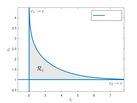
Figure 2: The geometry of 𝕎ε(|𝐲¯|)subscript𝕎subscript𝜀¯𝐲\mathbb{W}_{\mathfrak{R}_{\varepsilon}(|\overline{\mathbf{y}}|)} is depicted in two dimensions. Since ε1+ε2=εsubscript𝜀1subscript𝜀2𝜀\varepsilon_{1}+\varepsilon_{2}=\varepsilon, if ε1εsubscript𝜀1superscript𝜀\varepsilon_{1}\rightarrow\varepsilon^{-}, then ε20+subscript𝜀2superscript0\varepsilon_{2}\rightarrow 0^{+}, and vice versa. This shows that 𝕎ε(|𝐲¯|)subscript𝕎subscript𝜀¯𝐲\mathbb{W}_{\mathfrak{R}_{\varepsilon}(|\overline{\mathbf{y}}|)} is bounded.

Figure 2 illustrates geometric shape of 𝕎ε(|𝐲¯|)subscript𝕎subscript𝜀¯𝐲\mathbb{W}_{\mathfrak{R}_{\varepsilon}(|\overline{\mathbf{y}}|)} for q=2𝑞2q=2. The set of solutions that constitute 𝓡ε(|𝐲¯|)subscript𝓡𝜀¯𝐲\boldsymbol{\mathcal{R}}_{\varepsilon}(|\overline{\mathbf{y}}|) lies within a bounded set that is characterized by ε(|𝐲¯|)subscript𝜀¯𝐲\mathfrak{R}_{\varepsilon}(|\overline{\mathbf{y}}|).

When all output observables show evolution of similar stochastic events, a single safety margin can be employed to assess systemic risk throughout the network. For instance, all observables are similar or homogenous if every yksubscript𝑦𝑘y_{k}, for k=1,,q𝑘1𝑞k=1,\ldots,q, measures either deviation of a single state from the average of all states, pairwise difference between two agents, or deviation of a single state from average of its immediate neighbors. In this case, systemic risk measure becomes scalar-valued according to

ε(|𝐲¯|)=inf{δ+|(|𝐲¯|δ𝟙q)1ε}.subscript𝜀¯𝐲infimumconditional-set𝛿subscriptprecedes-or-equals¯𝐲𝛿subscript1𝑞1𝜀\mathcal{R}_{\varepsilon}(|\overline{\mathbf{y}}|)=\inf\Big{\{}\delta\in{\mathbb{R}}_{+}\leavevmode\nobreak\ \Big{|}\leavevmode\nobreak\ \mathbb{P}\big{(}\hskip 1.42271pt|\overline{\mathbf{y}}|\preceq\delta\mathbbm{1}_{q}\hskip 1.42271pt\big{)}\geq 1-\varepsilon\Big{\}}. (31)

The next result is a direct consequence of Theorem 4.

Corollary 1.

The scalar-valued joint systemic risk measure (31) for dynamical network (6) with observables (27) is bounded by

max1iqε(|y¯i|)ε(|𝐲¯|)min1iqυiε(|y¯i|)subscript1𝑖𝑞subscript𝜀subscript¯𝑦𝑖subscript𝜀¯𝐲subscript1𝑖𝑞subscript𝜐𝑖subscript𝜀subscript¯𝑦𝑖\max_{1\leq i\leq q}\hskip 1.42271pt\mathcal{R}_{\varepsilon}(|\overline{y}_{i}|)\leavevmode\nobreak\ \leq\leavevmode\nobreak\ {\mathcal{R}}_{\varepsilon}(|\overline{\mathbf{y}}|)\leavevmode\nobreak\ \leq\leavevmode\nobreak\ \hskip 1.42271pt\min_{1\leq i\leq q}\hskip 1.42271pt\upsilon_{i}\hskip 1.42271pt\mathcal{R}_{\varepsilon}(|\overline{y}_{i}|) (32)

where υi=Sε(0)1Sεi(0)subscript𝜐𝑖subscript𝑆𝜀superscript01subscript𝑆subscript𝜀𝑖0\upsilon_{i}=S_{\varepsilon}(0)^{-1}S_{\varepsilon_{i}}(0) for all positive εisubscript𝜀𝑖\varepsilon_{i}’s that satisfy (30).

{textblock*}

(11.3cm,-14.2cm) 𝕎εsubscript𝕎subscript𝜀\partial\mathbb{W}_{\mathfrak{R}_{\varepsilon}}

8.2 Risk of Large Fluctuations in Expectation

Suppose that function v:q:𝑣superscript𝑞v:{\mathbb{R}}^{q}\rightarrow{\mathbb{R}} is convex and monotonically increasing on the cone of positive orthant, i.e., if 𝒙𝒚precedes-or-equals𝒙𝒚\boldsymbol{x}\preceq\boldsymbol{y}, then v(𝒙)u(𝒚)𝑣𝒙𝑢𝒚v(\boldsymbol{x})\leq u(\boldsymbol{y}). The joint risk in expectation is an operator 𝓣ε:𝕃2(q)q:subscript𝓣𝜀superscript𝕃2superscript𝑞superscript𝑞\boldsymbol{\mathcal{T}}_{\varepsilon}:\mathbb{L}^{2}(\mathbb{R}^{q})\rightarrow\mathbb{R}^{q} that is defined by

𝓣ε(|𝐲¯|)=inf{𝜹q|𝔼[u(|𝐲¯|𝜹)]v(ε)},subscript𝓣𝜀¯𝐲infimumconditional-set𝜹superscript𝑞𝔼delimited-[]𝑢¯𝐲𝜹𝑣𝜀\boldsymbol{\mathcal{T}}_{\varepsilon}(|\overline{\mathbf{y}}|)=\inf\Big{\{}\boldsymbol{\delta}\in\mathbb{R}^{q}\leavevmode\nobreak\ \Big{|}\leavevmode\nobreak\ \mathbb{E}\big{[}u(|\overline{\mathbf{y}}|-\boldsymbol{\delta})\big{]}\leq v(\varepsilon)\Big{\}}, (33)

where 𝜹=[δ1,,δq]T𝜹superscriptsubscript𝛿1subscript𝛿𝑞𝑇\boldsymbol{\delta}=[\hskip 1.42271pt\delta_{1},\dots,\delta_{q}\hskip 1.42271pt]^{T} is the vector of safety margins.

Theorem 5.

Let us assume that 𝟙nker(C)subscript1𝑛kernel𝐶\mathbbm{1}_{n}\in\ker(C) for dynamical network (6) with observables (27). The constraint 𝔼[v(|𝐲¯|𝛅)]v(ε)𝔼delimited-[]𝑣¯𝐲𝛅𝑣𝜀\mathbb{E}\big{[}v(|\overline{\mathbf{y}}|-\boldsymbol{\delta})\big{]}\leq v(\varepsilon) in (33) with v(𝐳)=𝐳T𝐳𝑣𝐳superscript𝐳𝑇𝐳v(\boldsymbol{z})=\boldsymbol{z}^{T}\boldsymbol{z}, is feasible if and only if r>0𝑟0r>0 in which

r=ε2(12π)i=1qσ¯i2.𝑟superscript𝜀212𝜋superscriptsubscript𝑖1𝑞superscriptsubscript¯𝜎𝑖2r=\varepsilon^{2}-\bigg{(}1-\frac{2}{\pi}\bigg{)}\sum_{i=1}^{q}\hskip 1.42271pt\overline{\sigma}_{i}^{2}.

Moreover, the joint risk in expectation assumes a set value that is given by

𝓣ε(|𝐲¯|)={2π𝝈¯+𝐳|𝒛𝟎:𝐳=r}q,subscript𝓣𝜀¯𝐲conditional-set2𝜋¯𝝈𝐳:precedes-or-equals𝒛0norm𝐳𝑟superscript𝑞\boldsymbol{\mathcal{T}}_{\varepsilon}(|\overline{\mathbf{y}}|)=\left\{\hskip 1.42271pt\sqrt{\frac{2}{\pi}}\hskip 1.42271pt\overline{\boldsymbol{\sigma}}+\mathbf{z}\leavevmode\nobreak\ \bigg{|}\leavevmode\nobreak\ \boldsymbol{z}\preceq\boldsymbol{0}:\leavevmode\nobreak\ \|\mathbf{z}\|=\sqrt{r}\hskip 1.42271pt\right\}\subset{\mathbb{R}}^{q},

where 𝛔¯=[σ¯1,,σ¯q]T¯𝛔superscriptsubscript¯𝜎1subscript¯𝜎𝑞𝑇\overline{\boldsymbol{\sigma}}=[\hskip 1.42271pt\overline{\sigma}_{1},\ldots,\overline{\sigma}_{q}\hskip 1.42271pt]^{T}.

Theorem 6.

Suppose that assumptions of Theorem 5 hold. For all safety margins ε1,,εq>0subscript𝜀1subscript𝜀𝑞0\varepsilon_{1},\ldots,\varepsilon_{q}>0 that satisfy

ε12++εq2=ε2superscriptsubscript𝜀12superscriptsubscript𝜀𝑞2superscript𝜀2\varepsilon_{1}^{2}+\ldots+\varepsilon_{q}^{2}=\varepsilon^{2}

we have that

[𝒯ε1(|y¯1|),,𝒯εq(|y¯q|)]T𝓣ε(|𝐲¯|).superscriptsubscript𝒯subscript𝜀1subscript¯𝑦1subscript𝒯subscript𝜀𝑞subscript¯𝑦𝑞𝑇subscript𝓣𝜀¯𝐲\big{[}\mathcal{T}_{\varepsilon_{1}}(|\overline{y}_{1}|)\hskip 1.42271pt,\hskip 1.42271pt\ldots\hskip 1.42271pt,\hskip 1.42271pt\mathcal{T}_{\varepsilon_{q}}(|\overline{y}_{q}|)\big{]}^{T}\leavevmode\nobreak\ \in\leavevmode\nobreak\ \boldsymbol{\mathcal{T}}_{\varepsilon}(|\overline{\mathbf{y}}|).

When all observed stochastic events are homogeneous, the joint risk in expectation (33) reduces to a scalar as follows

𝒯ε(|𝐲¯|)=inf{δ|𝔼[v(|𝐲¯|δ𝟙q)]v(ε)}.subscript𝒯𝜀¯𝐲infimumconditional-set𝛿𝔼delimited-[]𝑣¯𝐲𝛿subscript1𝑞𝑣𝜀\mathcal{T}_{\varepsilon}(|\overline{\mathbf{y}}|)=\inf\Big{\{}\delta\in\mathbb{R}\leavevmode\nobreak\ \Big{|}\leavevmode\nobreak\ \mathbb{E}\big{[}v(|\overline{\mathbf{y}}|-\delta\mathbbm{1}_{q})\big{]}\leq v(\varepsilon)\Big{\}}. (34)

The risk measure 𝒯ε(|𝐲¯|)subscript𝒯𝜀¯𝐲\mathcal{T}_{\varepsilon}(|\overline{\mathbf{y}}|) is the smallest number δ𝛿\delta that can be added to every element of vector |𝐲¯|¯𝐲|\overline{\mathbf{y}}| such that the cost of the resulting vector stays below the predetermined safety threshold.

Corollary 2.

Let us assume that 𝟙nker(C)subscript1𝑛kernel𝐶\mathbbm{1}_{n}\in\ker(C) for dynamical network (6) with observable (27). Let ε2>jσ¯j22π(jσ¯j)2superscript𝜀2subscript𝑗superscriptsubscript¯𝜎𝑗22𝜋superscriptsubscript𝑗subscript¯𝜎𝑗2\varepsilon^{2}>\sum_{j}\overline{\sigma}_{j}^{2}-\frac{2}{\pi}\big{(}\sum_{j}\overline{\sigma}_{j}\big{)}^{2}, for σ¯jsubscript¯𝜎𝑗\overline{\sigma}_{j} the standard deviation of y¯jsubscript¯𝑦𝑗\overline{y}_{j}. Then, the risk in expectation as in (34) with quadratic utility function satisfies

𝒯ε(|𝐲¯|)=2πj=1qσ¯jε2j=1qσ¯j2+2π(j=1qσ¯j)2.subscript𝒯𝜀¯𝐲2𝜋superscriptsubscript𝑗1𝑞subscript¯𝜎𝑗superscript𝜀2superscriptsubscript𝑗1𝑞subscriptsuperscript¯𝜎2𝑗2𝜋superscriptsuperscriptsubscript𝑗1𝑞subscript¯𝜎𝑗2\mathcal{T}_{\varepsilon}\big{(}|\overline{\mathbf{y}}|\big{)}=\sqrt{\frac{2}{\pi}}\sum_{j=1}^{q}\overline{\sigma}_{j}-\sqrt{\varepsilon^{2}-\sum_{j=1}^{q}\overline{\sigma}^{2}_{j}+\frac{2}{\pi}\bigg{(}\sum_{j=1}^{q}\overline{\sigma}_{j}\bigg{)}^{2}}.

For vector-valued risk measure in expectation w.r.t. exponential utility function, we may use utility function

v(𝒛)=eβ(z1++zq).𝑣𝒛superscript𝑒𝛽subscript𝑧1subscript𝑧𝑞v(\boldsymbol{z})=e^{\beta(z_{1}+\ldots+z_{q})}.

The definition of risk measure in this case is given by

𝒯ε(|𝐲¯|)=inf{𝜹q|𝔼[eβi(|y¯i|δi)]eβε}.subscript𝒯𝜀¯𝐲infimumconditional-set𝜹superscript𝑞𝔼delimited-[]superscript𝑒𝛽subscript𝑖subscript¯𝑦𝑖subscript𝛿𝑖superscript𝑒𝛽𝜀\mathcal{T}_{\varepsilon}(|\mathbf{\overline{y}}|)=\inf\Big{\{}\boldsymbol{\delta}\in\mathbb{R}^{q}\leavevmode\nobreak\ \Big{|}\leavevmode\nobreak\ \mathbb{E}\big{[}e^{\beta\sum_{i}(|\overline{y}_{i}|-\delta_{i})}\big{]}\leq e^{\beta\varepsilon}\Big{\}}. (35)

Following a simple continuity argument, it can be shown that the vector of risk 𝒯ε(|𝐲¯|)=𝜹=(δ1,,δq)subscript𝒯𝜀¯𝐲𝜹subscript𝛿1subscript𝛿𝑞\mathcal{T}_{\varepsilon}(|\mathbf{\overline{y}}|)=\boldsymbol{\delta}=(\delta_{1},\dots,\delta_{q}) satisfies

i=1qδi=1βln(𝔼[eβ(i(|y¯i|1qε)])\sum_{i=1}^{q}\delta_{i}=\frac{1}{\beta}\ln\left(\mathbb{E}\Big{[}e^{\beta\big{(}\sum_{i}(|\overline{y}_{i}|-\frac{1}{q}\varepsilon\big{)}}\Big{]}\right) (36)

The calculation of the right hand side of (36) becomes significantly harder as it involves calculation of functions of joint random variables, which is beyond the scope of this paper.

Remark 4.

The vector-valued risk metrics, enjoy similar functional properties with the scalar risk metrics of §5. Indeed, Propositions 1 and 2 can be appropriately modified and extended to vector-valued risk, along the lines of [18]. The details are omitted due to space limitation.

9 Fundamental Limits and Tradeoffs

The presence of time-delay induces fundamental limits and tradeoffs on the least achievable risk values for the class of dynamical network (6) in steady-state. We characterize some Heisenberg-like inequalities and reveal inherent interplay between the systemic risk measure and a measure of network connectivity.

The first limit occurs due to stability condition of Assumption 2 that can be quantified as the following lower bound on the total effective resistance of the coupling graph of the network

Ξ𝒢>2n(n1)τπ.subscriptΞ𝒢2𝑛𝑛1𝜏𝜋\Xi_{\mathcal{G}}>\frac{2n(n-1)\tau}{\pi}. (37)

This implies that in time-delay network (6) the feedback structure (represented by the weighted graph 𝒢𝒢{\mathcal{G}}) may not have an overall strong couplings beyond the above limit, e.g., feedback loops may not have very large gains and/or dense topology especially when all gains are equal (which corresponds to unweighted 𝒢𝒢{\mathcal{G}}).

Refer to caption
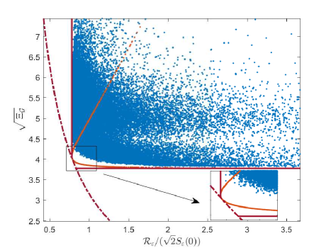
Figure 3: Fundamental and trade-off bound curves for the systemic risk. Blue dots are randomly generated graphs over n=8𝑛8n=8 agents, for fixed τ=0.4𝜏0.4\tau=0.4 and output vector 𝐜𝐜\mathbf{c}. The red vertical and horizontal lines are the hard limits, and the dashed line is the trade-off principle. The orange curve illustrates a particular family of graphs that achieve the trade-off curve, asserting that all three bounds are sharp.
Theorem 7.

Let observable of dynamical network (6) be scalar as in (14), i.e., q=1𝑞1q=1. Then, there is a hard limit on the least achievable value for risk of large fluctuations as follows

ε(|y¯|)κτsubscript𝜀¯𝑦subscript𝜅𝜏\mathcal{R}_{\varepsilon}(|\overline{y}|)\hskip 1.42271pt\geq\hskip 1.42271pt\kappa_{*}\hskip 1.42271pt\sqrt{\tau} (38)

where

κ=𝐜bSε(0)1sin(z+)subscript𝜅norm𝐜𝑏subscript𝑆𝜀01superscript𝑧\kappa_{*}=\|\mathbf{c}\|\hskip 1.42271pt\frac{b\hskip 1.42271ptS_{\varepsilon}(0)}{\sqrt{1-\sin(z^{+})}}

and z+superscript𝑧z^{+} is the positive solution of equation cos(z)=z𝑧𝑧\cos(z)=z. Furthermore, the least achievable value for risk of high volatility cannot be improved beyond some lower bound that is characterized by:

  • (a)

    for quadratic utility function:

    𝒯ε(|y¯|)2πσε2(12π)σ2subscript𝒯𝜀¯𝑦2𝜋subscript𝜎superscript𝜀212𝜋superscriptsubscript𝜎2\mathcal{T}_{\varepsilon}(|\overline{y}|)\geq\sqrt{\frac{2}{\pi}}\sigma_{*}-\sqrt{\varepsilon^{2}-\bigg{(}1-\frac{2}{\pi}\bigg{)}\sigma_{*}^{2}}
  • (b)

    for exponential utility function:

    𝒯ε(|y¯|)βσ22+ln(1+erf(βσ2))βεsubscript𝒯𝜀¯𝑦𝛽superscriptsubscript𝜎221erf𝛽subscript𝜎2𝛽𝜀\begin{split}\mathcal{T}_{\varepsilon}(|\overline{y}|)\geq\frac{\beta\sigma_{*}^{2}}{2}&+\frac{\ln\big{(}1+\mathrm{erf}(\frac{\beta\sigma_{*}}{2})\big{)}}{\beta}-\varepsilon\end{split}

where

σ=b𝐜τ2(1sin(z+)).subscript𝜎𝑏delimited-∥∥𝐜𝜏21superscript𝑧\begin{split}\sigma_{*}=b\hskip 1.42271pt\|\mathbf{c}\|\hskip 1.42271pt\sqrt{\frac{\tau}{2\big{(}1-\sin(z^{+})\big{)}}}.\end{split} (39)

The lower limit can be achieved by graphs with Laplacian spectrum that satisfy λiτ=z+subscript𝜆𝑖𝜏superscript𝑧\lambda_{i}\tau=z^{+} for all i>1𝑖1i>1, i.e., a complete graph over n𝑛n nodes with coupling weights kij0.7391nτsubscript𝑘𝑖𝑗0.7391𝑛𝜏k_{ij}\approx\frac{0.7391}{n\tau}. Inequalities (37) and (38) represent hard limits as their lower bounds are independent of the coupling structure of the network; by fixing ε𝜀\varepsilon they only depend on the size of the network and time-delay. When there is no time-delay, i.e., τ=0𝜏0\tau=0, hard limits disappear. Because in no time delay case, one may simultaneously improve risk and connectivity by arbitrarily increasing the feedback gains. This shows that time-delay is the main reason for emergence of these fundamental limits on risk and connectivity.

Theorem 8.

Let observable of dynamical network (6) be scalar, i.e., q=1𝑞1q=1. There is an inherent fundamental tradeoff between least achievable values for risk of large fluctuations and network interconnectivity that can be quantified as follows

ε(|y¯|)Ξ𝒢>ϑnτsubscript𝜀¯𝑦subscriptΞ𝒢subscriptitalic-ϑ𝑛𝜏\mathcal{R}_{\varepsilon}(|\overline{y}|)\hskip 1.42271pt\cdot\hskip 1.42271pt\sqrt{\Xi_{\mathcal{G}}}\hskip 1.42271pt>\hskip 1.42271pt\vartheta_{*}\hskip 1.42271pt\sqrt{n\tau} (40)

where Ξ𝒢subscriptΞ𝒢\Xi_{\mathcal{G}} is the total effective resistance of the coupling graph of the network and

ϑ=𝐜bSε(0)psubscriptitalic-ϑnorm𝐜𝑏subscript𝑆𝜀0superscript𝑝\vartheta_{*}\hskip 1.42271pt=\hskip 1.42271pt\|\mathbf{c}\|\hskip 1.42271ptb\hskip 1.42271ptS_{\varepsilon}(0)\hskip 1.42271pt\sqrt{p^{\dagger}}

with p=min{p2,,pn}superscript𝑝superscriptsubscript𝑝2superscriptsubscript𝑝𝑛p^{\dagger}=\min\{p_{2}^{*},\ldots,p_{n}^{*}\} in which positive numbers pksuperscriptsubscript𝑝𝑘p_{k}^{*} is the minimum of

pk(x)=[(k1)+2(nk)πx]cos(x)x2(1sin(x))subscript𝑝𝑘𝑥delimited-[]𝑘12𝑛𝑘𝜋𝑥𝑥superscript𝑥21𝑥p_{k}(x)=\bigg{[}(k-1)+\frac{2(n-k)}{\pi}x\bigg{]}\frac{\cos(x)}{x^{2}(1-\sin(x))}

over x(0,π/2)𝑥0𝜋2x\in(0,\pi/2) for all k=2,,n𝑘2𝑛k=2,\dots,n. Moreover, fundamental tradeoffs emerge between the least achievable values for volatility risk and network connectivity in the following sense

(𝒯ε(|y¯|)+ε)Ξ𝒢>Δ(τ)subscript𝒯𝜀¯𝑦𝜀subscriptΞ𝒢Δ𝜏\big{(}\mathcal{T}_{\varepsilon}(|\overline{y}|)+\varepsilon\big{)}\sqrt{\Xi_{\mathcal{G}}}\hskip 1.42271pt>\hskip 1.42271pt\Delta(\tau)

in which

Δ(τ)=(2π+12ε(12π)σ)ϱΔ𝜏2𝜋12𝜀12𝜋subscript𝜎subscriptitalic-ϱ\Delta(\tau)=\bigg{(}\sqrt{\frac{2}{\pi}}+\frac{1}{2\varepsilon}\bigg{(}1-\frac{2}{\pi}\bigg{)}\sigma_{*}\bigg{)}\varrho_{*}

for the quadratic utility function and

Δ(τ)=β2σϱ+erf(βσ/2)βn(n1)τπΔ𝜏𝛽2subscript𝜎subscriptitalic-ϱerf𝛽subscript𝜎2𝛽𝑛𝑛1𝜏𝜋\Delta(\tau)=\frac{\beta}{2}\sigma_{*}\varrho_{*}+\frac{\mathrm{erf}(\beta\sigma_{*}/2)}{\beta}\hskip 1.42271pt\frac{n(n-1)\tau}{\pi}

for the exponential utility function, where

ϱ=𝐜|b|nτ2p.subscriptitalic-ϱnorm𝐜𝑏𝑛𝜏2superscript𝑝\varrho_{*}\hskip 1.42271pt=\hskip 1.42271pt\|\mathbf{c}\|\hskip 1.42271pt|b|\hskip 1.42271pt\sqrt{\frac{n\tau}{2}p^{\dagger}}. (41)
Graph Risk of Large Fluctuations in Probability for Scalar Events
𝐊nsubscript𝐊𝑛\mathbf{K}_{n} ε(|y¯i|)=2Sε(0)τ(11n)f(nτ)fori=1,,nformulae-sequencesubscript𝜀subscript¯𝑦𝑖2subscript𝑆𝜀0𝜏11𝑛𝑓𝑛𝜏for𝑖1𝑛\mathcal{R}_{\varepsilon}(|\overline{y}_{i}|)=\sqrt{2}S_{\varepsilon}(0)\sqrt{\tau\left(1-\frac{1}{n}\right)f(n\tau)}\leavevmode\nobreak\ \leavevmode\nobreak\ \leavevmode\nobreak\ \leavevmode\nobreak\ \textrm{for}\leavevmode\nobreak\ \leavevmode\nobreak\ i=1,\dots,n
𝐖n+1subscript𝐖𝑛1\mathbf{W}_{n+1} ε(|y¯|i)=2Sε(0)×{nτf((n+1)τ)ifi=1τnk=2n+1f(32cos(2π(k1)τn))ifi=2,,nsubscript𝜀subscript¯𝑦𝑖2subscript𝑆𝜀0cases𝑛𝜏𝑓𝑛1𝜏if𝑖1𝜏𝑛superscriptsubscript𝑘2𝑛1𝑓322𝜋𝑘1𝜏𝑛formulae-sequenceif𝑖2𝑛\mathcal{R}_{\varepsilon}(|\overline{y}|_{i})=\sqrt{2}S_{\varepsilon}(0)\times\begin{cases}\sqrt{n\tau f\big{(}(n+1)\tau\big{)}}&\leavevmode\nobreak\ \leavevmode\nobreak\ \textrm{if}\leavevmode\nobreak\ \leavevmode\nobreak\ i=1\\ \sqrt{\frac{\tau}{n}\leavevmode\nobreak\ \displaystyle\sum_{k=2}^{n+1}f\left(3-2\cos\left(\frac{2\pi(k-1)\tau}{n}\right)\right)}&\leavevmode\nobreak\ \leavevmode\nobreak\ \textrm{if}\leavevmode\nobreak\ \leavevmode\nobreak\ i=2,\dots,n\end{cases}
𝐊n1,n2subscript𝐊subscript𝑛1subscript𝑛2\mathbf{K}_{n_{1},n_{2}} ε(|y¯|i)=2Sε(0)×{(11n2)τf(n2τ)+n2n1nτf(nτ)ifi𝒢1(11n1)τf(n1τ)+n1n2nτf(nτ)ifi𝒢2subscript𝜀subscript¯𝑦𝑖2subscript𝑆𝜀0cases11subscript𝑛2𝜏𝑓subscript𝑛2𝜏subscript𝑛2subscript𝑛1𝑛𝜏𝑓𝑛𝜏if𝑖subscript𝒢111subscript𝑛1𝜏𝑓subscript𝑛1𝜏subscript𝑛1subscript𝑛2𝑛𝜏𝑓𝑛𝜏if𝑖subscript𝒢2\mathcal{R}_{\varepsilon}(|\overline{y}|_{i})=\sqrt{2}S_{\varepsilon}(0)\times\begin{cases}\sqrt{\big{(}1-\frac{1}{n_{2}}\big{)}\tau f(n_{2}\tau)+\frac{n_{2}}{n_{1}n}\tau f(n\tau)}&\leavevmode\nobreak\ \leavevmode\nobreak\ \textrm{if}\leavevmode\nobreak\ \leavevmode\nobreak\ i\in{\mathcal{G}}_{1}\\ \sqrt{\big{(}1-\frac{1}{n_{1}}\big{)}\tau f(n_{1}\tau)+\frac{n_{1}}{n_{2}n}\tau f(n\tau)}&\leavevmode\nobreak\ \leavevmode\nobreak\ \textrm{if}\leavevmode\nobreak\ \leavevmode\nobreak\ i\in{\mathcal{G}}_{2}\end{cases}
𝐏nsubscript𝐏𝑛\mathbf{P}_{n} ε(|y¯|i)=2Sε(0)2τnk=2ncos2(π(nk+1)(2i1)2n)f(2[1cos(π(k1)n)]τ),i=1,,nformulae-sequencesubscript𝜀subscript¯𝑦𝑖2subscript𝑆𝜀02𝜏𝑛superscriptsubscript𝑘2𝑛superscript2𝜋𝑛𝑘12𝑖12𝑛𝑓2delimited-[]1𝜋𝑘1𝑛𝜏𝑖1𝑛\mathcal{R}_{\varepsilon}(|\overline{y}|_{i})=\sqrt{2}S_{\varepsilon}(0)\displaystyle\sqrt{\frac{2\tau}{n}\sum_{k=2}^{n}\cos^{2}\left(\frac{\pi(n-k+1)(2i-1)}{2n}\right)f\left(2\left[1-\cos\left(\frac{\pi(k-1)}{n}\right)\right]\tau\right)},\leavevmode\nobreak\ i=1,\dots,n
𝐑nsubscript𝐑𝑛\mathbf{R}_{n} ε(|y¯|i)=2Sε(0)τk=2nf(2[1cos(2π(k1)n)]τ),i=1,,nformulae-sequencesubscript𝜀subscript¯𝑦𝑖2subscript𝑆𝜀0𝜏superscriptsubscript𝑘2𝑛𝑓2delimited-[]12𝜋𝑘1𝑛𝜏𝑖1𝑛\mathcal{R}_{\varepsilon}(|\overline{y}|_{i})=\sqrt{2}S_{\varepsilon}(0)\sqrt{\tau\displaystyle\sum_{k=2}^{n}f\left(2\left[1-\cos\left(\frac{2\pi(k-1)}{n}\right)\right]\tau\right)},\leavevmode\nobreak\ i=1,\dots,n
Table 1: Explicit formulas for systemic risk measure of individual events. The function f(x)𝑓𝑥f(x) is defined in (10). For a detailed analysis on the derivation of the formulas we refer to Appendix C.

Inequality (40) implies that network (6) will be prone to higher levels of risk if the connectivity enhances, e.g., by adding new coupling links and/or increasing the feedback gains. The origin of this intrinsic tradeoff is time-delay; inequality (40) would be trivial if τ=0𝜏0\tau=0. We observe that by increasing τ𝜏\tau, while preserving stability, interplay between systemic risk and network connectivity becomes more apparent. The key observation is that by fixing the network size, time delay and ε𝜀\varepsilon inequalities (38) and (40) remain true for all dynamical networks (6) with arbitrary graph topologies and output matrices c𝑐c; in other words, these fundamental limits and tradeoffs are universal. In Figure 3, we verify tightness of our bounds using extensive simulation results. The blue dots are numerically calculated based on the following procedure: (i) randomly generate a connected graph that satisfies stability condition in Assumption 2 , (ii) randomly generate an output vector c𝑐c, and (iii) compute the scaled pair (Ξ𝒢,ε(y¯))/(2Sε(0))subscriptΞ𝒢subscript𝜀¯𝑦2subscript𝑆𝜀0(\sqrt{\Xi_{\mathcal{G}}},\mathcal{R}_{\varepsilon}(\bar{y}))/(\sqrt{2}S_{\varepsilon}(0)). The orange color curve in Figure 3 illustrates a particular family of complete graphs with parametrized identical coupling strengths that is specifically constructed to highlight sharpness of our bounds in (38) and (40).

Theorem 9.

Let us consider dynamical network (6) with vector of observables (27). There is an intrinsic fundamental tradeoff between the least achievable values for the joint vector-valued risk measure on +qsubscriptsuperscript𝑞{\mathbb{R}}^{q}_{+} and network interconnectivity that can be characterized by inequality

𝓡ε(|𝐲¯|)Ξ𝒢𝚯nτsucceedssubscript𝓡𝜀¯𝐲subscriptΞ𝒢subscript𝚯𝑛𝜏\boldsymbol{\mathcal{R}}_{\varepsilon}(|\overline{\mathbf{y}}|)\hskip 1.42271pt\cdot\hskip 1.42271pt\sqrt{\Xi_{\mathcal{G}}}\hskip 1.42271pt\succ\hskip 1.42271pt\boldsymbol{\Theta}_{*}\hskip 1.42271pt\sqrt{n\tau} (42)

in which 𝚯=bSε(0)p[𝐜1,,𝐜q]T.subscript𝚯𝑏subscript𝑆𝜀0superscript𝑝superscriptnormsubscript𝐜1normsubscript𝐜𝑞𝑇\boldsymbol{\Theta}_{*}=b\hskip 1.42271ptS_{\varepsilon}(0)\hskip 1.42271pt\sqrt{p^{\dagger}}\leavevmode\nobreak\ \big{[}\hskip 1.42271pt\|\mathbf{c}_{1}\|,\hskip 1.42271pt\ldots\hskip 1.42271pt,\|\mathbf{c}_{q}\|\hskip 1.42271pt\big{]}^{T}.

Proof of this theorem is based on results of Theorems 4 and 8 and is omitted.

Corollary 3.

Suppose that 𝟙nker(C)subscript1𝑛kernel𝐶\mathbbm{1}_{n}\in\ker(C) for dynamical network (6) with output matrix C=[𝐜1,,𝐜q]T𝐶superscriptsubscript𝐜1subscript𝐜𝑞𝑇C=\big{[}\hskip 1.42271pt\mathbf{c}_{1},\ldots,\mathbf{c}_{q}\hskip 1.42271pt\big{]}^{T}. The vector-valued joint risk in expectation (33) cannot be improved beyond some hard limits that are characterized as lower bounds in the following inequalities:

(i)𝑖(i) For quadratic utility function v(𝒛)=𝒛T𝒛𝑣𝒛superscript𝒛𝑇𝒛v(\boldsymbol{z})=\boldsymbol{z}^{T}\boldsymbol{z}, it follows that

𝓣ε(|𝐲¯|)2π𝝈¯ 1qε2(12π)𝝈¯2succeeds-or-equalssubscript𝓣𝜀¯𝐲2𝜋superscriptbold-¯𝝈subscript1𝑞superscript𝜀212𝜋superscriptnormsuperscriptbold-¯𝝈2\boldsymbol{\mathcal{T}}_{\varepsilon}(|\mathbf{\overline{y}}|)\leavevmode\nobreak\ \succeq\leavevmode\nobreak\ \sqrt{\frac{2}{\pi}}\hskip 1.42271pt\boldsymbol{\overline{\sigma}}^{*}\leavevmode\nobreak\ -\leavevmode\nobreak\ \mathbbm{1}_{q}\leavevmode\nobreak\ \sqrt{\varepsilon^{2}-\bigg{(}1-\frac{2}{\pi}\bigg{)}\hskip 1.42271pt\|\boldsymbol{\overline{\sigma}}^{*}\|^{2}}

where 𝝈¯=[σ1,,σq]Tsuperscriptbold-¯𝝈superscriptsuperscriptsubscript𝜎1superscriptsubscript𝜎𝑞𝑇\boldsymbol{\overline{\sigma}}^{*}=[\hskip 1.42271pt\sigma_{1}^{*},\ldots,\sigma_{q}^{*}]^{T} with

σi=𝐜ibτ2(1sin(z+)),superscriptsubscript𝜎𝑖normsubscript𝐜𝑖𝑏𝜏21superscript𝑧\sigma_{i}^{*}=\|\mathbf{c}_{i}\|\hskip 1.42271ptb\hskip 1.42271pt\sqrt{\frac{\tau}{2\big{(}1-\sin(z^{+})\big{)}}},

and z+superscript𝑧z^{+} is the positive solution of equation cos(z)=z𝑧𝑧\cos(z)=z.

(ii)𝑖𝑖(ii) For exponential utility function v(𝒛)=eβ(z1++zq)𝑣𝒛superscript𝑒𝛽subscript𝑧1subscript𝑧𝑞v(\boldsymbol{z})=e^{\beta(z_{1}+\ldots+z_{q})}, it holds that

𝟙qT𝓣ε(|𝐲¯|)bτπ(1sin(z+))i=1q𝐜iε.superscriptsubscript1𝑞𝑇subscript𝓣𝜀¯𝐲𝑏𝜏𝜋1superscript𝑧superscriptsubscript𝑖1𝑞normsubscript𝐜𝑖𝜀\mathbbm{1}_{q}^{T}\boldsymbol{\mathcal{T}}_{\varepsilon}(|\mathbf{\overline{y}}|)\leavevmode\nobreak\ \geq\leavevmode\nobreak\ b\leavevmode\nobreak\ \sqrt{\frac{\tau}{\pi\big{(}1-\sin(z^{+})\big{)}}}\leavevmode\nobreak\ \sum_{i=1}^{q}\|\mathbf{c}_{i}\|-\varepsilon.

10 Exploiting Graph Topology

We show that for some graph topologies, the value of systemic risk measure can be calculated explicitly. Our focus will be only on risk in probability with respect to deviation of a single state from the average, where similar results can be obtained for other types of observations as well as risk in expectation. In order to exploit graph structure and determine how risk scales with network size, we consider the class of dynamical network (6) with unweighted coupling graphs. The results of this section are summarized in Table 1.

Complete graph. Due to the perfect symmetry of a complete graph 𝐊nsubscript𝐊𝑛\mathbf{K}_{n}, all elements of the vector of joint fluctuation risk measure are identical and the risk measure reduces to (31). The network is marginally stable if τ<π2n𝜏𝜋2𝑛\tau<\frac{\pi}{2n}, where this region shrinks as n𝑛n grows. For two given linear consensus networks (6) with coupling graphs 𝐊n1subscript𝐊subscript𝑛1\mathbf{K}_{n_{1}} and 𝐊n2subscript𝐊subscript𝑛2\mathbf{K}_{n_{2}} and n1<n2subscript𝑛1subscript𝑛2n_{1}<n_{2}, there exists a critical time delay τ<π2n2superscript𝜏𝜋2subscript𝑛2\tau^{*}<\frac{\pi}{2n_{2}} such that ε(2)(|𝒚¯|)ε(1)(|𝒚¯|)subscriptsuperscript2𝜀¯𝒚superscriptsubscript𝜀1¯𝒚\mathcal{R}^{(2)}_{\varepsilon}(|\overline{\boldsymbol{y}}|)\leq\mathcal{R}_{\varepsilon}^{(1)}(|\overline{\boldsymbol{y}}|) for all ττ𝜏superscript𝜏\tau\leq\tau^{*}, and ε(1)(|𝒚¯|)<ε(2)(|𝒚¯|)subscriptsuperscript1𝜀¯𝒚superscriptsubscript𝜀2¯𝒚\mathcal{R}^{(1)}_{\varepsilon}(|\overline{\boldsymbol{y}}|)<\mathcal{R}_{\varepsilon}^{(2)}(|\overline{\boldsymbol{y}}|) for all τ<τ<π2n2superscript𝜏𝜏𝜋2subscript𝑛2\tau^{*}<\tau<\frac{\pi}{2n_{2}}. The phenomenon is graphically illustrated on the left plot of Figure 4. In a more simple language, networks with larger complete graphs are safer than smaller ones, and as time delay increases there is a transition point beyond which networks with smaller complete graphs are safer.

Wheel graph. Let us label the central node of the wheel graph 𝐖n+1subscript𝐖𝑛1\mathbf{W}_{n+1} by 111 and the remaining nodes on the circumference by 2,,n+12𝑛12,\ldots,n+1. The largest Laplacian eigenvalue is λn+1=n+1subscript𝜆𝑛1𝑛1\lambda_{n+1}=n+1, which implies that network is marginally stable if τ<π2(n+1)𝜏𝜋2𝑛1\tau<\frac{\pi}{2(n+1)}. The symmetric structure of 𝐖n+1subscript𝐖𝑛1\mathbf{W}_{n+1} implies that ε(|y¯2|)==ε(|y¯n+1|)subscript𝜀subscript¯𝑦2subscript𝜀subscript¯𝑦𝑛1\mathcal{R}_{\varepsilon}(|\overline{y}_{2}|)=\ldots=\mathcal{R}_{\varepsilon}(|\overline{y}_{n+1}|). According to explicit expressions for risk measures in Table 1, we can verify that555It can be shown that ε(|y¯|i)ε(|y¯|1)<1n2+n21n2cos(λτ)1sin(λτ)1sin((n+1)τ)cos((n+1)τ)1subscript𝜀subscript¯𝑦𝑖subscript𝜀subscript¯𝑦11superscript𝑛2superscript𝑛21superscript𝑛2superscript𝜆𝜏1superscript𝜆𝜏1𝑛1𝜏𝑛1𝜏1\begin{split}\frac{\mathcal{R}_{\varepsilon}(|\overline{y}|_{i})}{\mathcal{R}_{\varepsilon}(|\overline{y}|_{1})}&<\frac{1}{n^{2}}+\frac{n^{2}-1}{n^{2}}\frac{\cos(\lambda^{*}\tau)}{1-\sin(\lambda^{*}\tau)}\frac{1-\sin((n+1)\tau)}{\cos((n+1)\tau)}\leq 1\end{split} for all i=2,,n+1𝑖2𝑛1i=2,\ldots,n+1, where λsuperscript𝜆\lambda^{*} is the maximizer of cos(λτ)1sin(λτ)𝜆𝜏1𝜆𝜏\frac{\cos(\lambda\tau)}{1-\sin(\lambda\tau)} over λ{32cos(2π(k1)/n)|k=2,,n}𝜆conditional-set322𝜋𝑘1𝑛𝑘2𝑛\lambda\in\big{\{}3-2\cos(2\pi(k-1)/n)\leavevmode\nobreak\ |\leavevmode\nobreak\ k=2,\ldots,n\big{\}}. ε(|y¯|1)<ε(|y¯|i)subscript𝜀subscript¯𝑦1subscript𝜀subscript¯𝑦𝑖\mathcal{R}_{\varepsilon}(|\overline{y}|_{1})<\mathcal{R}_{\varepsilon}(|\overline{y}|_{i}) for all i=2,,n+1𝑖2𝑛1i=2,\ldots,n+1. Thus, the central node in a dynamical network with wheel graph is riskier than the surrounding nodes.
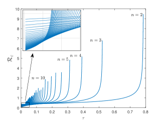
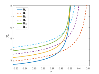
Refer to caption
Refer to caption
Figure 4: (Left) The fluctuation risk of a complete graph as a function of the delay τ𝜏\tau. Here ε=0.01𝜀0.01\varepsilon=0.01 and 𝐊nsubscript𝐊𝑛\mathbf{K}_{n}, n=2,,50𝑛250n=2,\dots,50. (Right) Fluctuation risk on ring graphs in terms of network size. A remarkable qualitative distinction appears between graphs with odd and graphs with even number of agents.

Complete Bipartite graph. Let us denote each side of the complete bipartite graph 𝐊n1,n2subscript𝐊subscript𝑛1subscript𝑛2\mathbf{K}_{n_{1},n_{2}} by 𝒢1subscript𝒢1{\mathcal{G}}_{1} and 𝒢2subscript𝒢2{\mathcal{G}}_{2} that each has n1subscript𝑛1n_{1} and n2subscript𝑛2n_{2} nodes, respectively. Nodes at each side are only connected to nodes on the other side. The total number of nodes is n=n1+n2𝑛subscript𝑛1subscript𝑛2n=n_{1}+n_{2} and let us assume that n1n2subscript𝑛1subscript𝑛2n_{1}\leq n_{2}. In this case, the network (6) is marginally stable if and only if τ<π2n𝜏𝜋2𝑛\tau<\frac{\pi}{2n}. The symmetric topology of 𝐊n1,n2subscript𝐊subscript𝑛1subscript𝑛2\mathbf{K}_{n_{1},n_{2}} entails that all ε(|y¯|i)subscript𝜀subscript¯𝑦𝑖\mathcal{R}_{\varepsilon}(|\overline{y}|_{i}) belonging to one side (either 𝒢1subscript𝒢1{\mathcal{G}}_{1} or 𝒢2subscript𝒢2{\mathcal{G}}_{2}) are identical. We may categorize the set of complete bipartite graphs into two subclasses: graphs with n1=1subscript𝑛11n_{1}=1 and the ones with n1>1subscript𝑛11n_{1}>1. The first class contains all star graphs 𝐊1,n1subscript𝐊1𝑛1\mathbf{K}_{1,n-1}, where 𝒢1subscript𝒢1{\mathcal{G}}_{1} consists of only node with label 111 and 𝒢2subscript𝒢2{\mathcal{G}}_{2} contains all nodes with labels 2,,n2𝑛2,\ldots,n. From Table 1, it is straightforward to verify that

ε(|y¯|1)>ε(|y¯|j)subscript𝜀subscript¯𝑦1subscript𝜀subscript¯𝑦𝑗\mathcal{R}_{\varepsilon}(|\overline{y}|_{1})>\mathcal{R}_{\varepsilon}(|\overline{y}|_{j})

for all nodes j{2,,n}𝑗2𝑛j\in\{2,\ldots,n\} in subgraph 𝒢2subscript𝒢2{\mathcal{G}}_{2}. Similar to the wheel graph, the central node in a star graph attains the highest risk value among all nodes in the network, regardless of the time delay value. When n1>1subscript𝑛11n_{1}>1, from Table 1 and some elementary analysis, it can be shown that there exists a unique τ=τ(n1,n2)superscript𝜏superscript𝜏subscript𝑛1subscript𝑛2\tau^{*}=\tau^{*}(n_{1},n_{2}) such that for all i𝑖i in subgraph 𝒢1subscript𝒢1{\mathcal{G}}_{1} and all j𝑗j in subgraph 𝒢2subscript𝒢2{\mathcal{G}}_{2} the following inequalities hold

ε(|y¯|i)ε(|y¯|j)for 0ττε(|y¯|j)<ε(|y¯|i)forτ<τ<π2n.formulae-sequenceformulae-sequencesubscript𝜀subscript¯𝑦𝑖subscript𝜀subscript¯𝑦𝑗for 0𝜏superscript𝜏subscript𝜀subscript¯𝑦𝑗subscript𝜀subscript¯𝑦𝑖forsuperscript𝜏𝜏𝜋2𝑛\begin{split}\mathcal{R}_{\varepsilon}(|\overline{y}|_{i})&\leq\mathcal{R}_{\varepsilon}(|\overline{y}|_{j})\leavevmode\nobreak\ \leavevmode\nobreak\ \leavevmode\nobreak\ \textrm{for}\leavevmode\nobreak\ \leavevmode\nobreak\ \leavevmode\nobreak\ 0\leq\tau\leq\tau^{*}\\ \mathcal{R}_{\varepsilon}(|\overline{y}|_{j})&<\mathcal{R}_{\varepsilon}(|\overline{y}|_{i})\leavevmode\nobreak\ \leavevmode\nobreak\ \leavevmode\nobreak\ \textrm{for}\leavevmode\nobreak\ \leavevmode\nobreak\ \leavevmode\nobreak\ \tau^{*}<\tau<\frac{\pi}{2n}.\end{split}

For n1>1subscript𝑛11n_{1}>1, we conclude that, unlike graphs with star topology, time delay plays an active role in determining which of the subgraphs 𝒢1subscript𝒢1{\mathcal{G}}_{1} or 𝒢2subscript𝒢2{\mathcal{G}}_{2} contains riskier nodes. This point is illustrated with two examples in Figure 5.
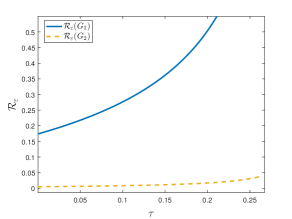
Refer to caption
Refer to caption
Figure 5: Illustration of the systemic risk on 𝐊1,4subscript𝐊14\mathbf{K}_{1,4} and 𝐊2,8subscript𝐊28\mathbf{K}_{2,8}. The first example is the star graph. The central node is the riskier one. The second scheme has a group of two and eight nodes, respectively. In the second scheme, we observe that the larger group is safer for small delay and riskier for large delay.
Refer to caption
Refer to caption
Figure 6: Systemic risk for 𝐏6subscript𝐏6\mathbf{P}_{6} and 𝐏7subscript𝐏7\mathbf{P}_{7}. For small delays, the risk increases monotonically for as nodes lie closer to the center, where as for large delays, the risk monotonically decreases. When n𝑛n is odd and τ𝜏\tau approaches the critical delay value, the risk of the central node increases towards infinity at a significantly lower rate than the rest of the network.

Path graph. In networks for which agents are connected to a uniformly bounded number of neighbors, such as path and ring graphs, the marginal stability range for time delay does not shrink to zero as the network size grows. A network with path graph topology 𝐏nsubscript𝐏𝑛\mathbf{P}_{n} is marginally stable iff τ<π4(1+cos(πn))𝜏𝜋41𝜋𝑛\tau<\frac{\pi}{4\left(1+\cos(\frac{\pi}{n})\right)}. A simple calculation reveals that the network is marginally stable for all n𝑛n iff τ<π8𝜏𝜋8\tau<\frac{\pi}{8}. From Table 1, it can be verified that

ε(|y¯|i)=ε(|y¯|ni+1)subscript𝜀subscript¯𝑦𝑖subscript𝜀subscript¯𝑦𝑛𝑖1\mathcal{R}_{\varepsilon}(|\overline{y}|_{i})=\mathcal{R}_{\varepsilon}(|\overline{y}|_{n-i+1})

for all i=1,,n𝑖1𝑛i=1,\ldots,n.

There exists a critical time delay τsuperscript𝜏\tau^{*} in the marginal stability range that for all time delays τ<τ𝜏superscript𝜏\tau<\tau^{*} agents residing toward the tails of the path graph are safer than the ones located closer to the center. In this case, central nodes are more prone to large fluctuations. When τ>τ𝜏superscript𝜏\tau>\tau^{*}, agents closer to the center become safer and the ones that are closer to the tails become riskier. In conclusion, agents residing in the boundaries are the safest for small time delays, and in contrary, agents located in the center are the safest for large time delays. When n𝑛n is odd, there is a central agent who becomes significantly safer for large time delays. Figure 6 illustrates these analytic design rules of thumb graphically.

Ring graph. The dynamical network (6) with ring graph topology 𝐑nsubscript𝐑𝑛\mathbf{R}_{n} is marginally stable iff

τ<π4(1cos(2π(11n)))1.𝜏𝜋4superscript12𝜋11𝑛1\tau<\frac{\pi}{4}\left(1-\cos\left(2\pi\left(1-\frac{1}{n}\right)\right)\right)^{-1}.

The symmetric structure of 𝐑nsubscript𝐑𝑛\mathbf{R}_{n} necessitates that all agents to have identical risk values. In the right plot of Figure 4, the value of the systemic risk measure for one of the agents, which is given in Table 1, is drawn for different values of n𝑛n. One observes that the systemic risk measure monotonically increases by n𝑛n for small time delays. However, when time delay increases and approaches the marginal stability border, networks with odd number of agents appear safer than networks with even number of agents.

11 Simulations

We verify our theoretical findings through two numerical examples.

Example 1.

(Transient Behavior of Risk Measures) Consider the graph over n=5𝑛5n=5 nodes as in Figure 7.

1234523.20.150.20.3
Figure 7: The graph for Example 1. The assigned weights accompany the edges between nodes, allow a maximum delay of τmax=0.1211subscript𝜏0.1211\tau_{\max}=0.1211.
Refer to caption
Refer to caption
Figure 8: Simulated (dot) and analytic (solid line) results for 𝐲t=C𝐱tsubscript𝐲𝑡𝐶subscript𝐱𝑡\mathbf{y}_{t}=C\mathbf{x}_{t}. Figure on the left illustrates the variances and figure on the right the volatility risk with quadratic utility. For t=4𝑡4t=4 to t=12𝑡12t=12, the variance of the orange observable lies above the permissible cut-off value. According to Theorem 1, its risk in quadratic volatility is infinite. Similarly for the motion of the average (the line) for t11𝑡11t\geq 11.
Refer to caption
Refer to caption
Figure 9: Simulated (dot) and analytic (solid line) results for 𝐲t=C𝐱tsubscript𝐲𝑡𝐶subscript𝐱𝑡\mathbf{y}_{t}=C\mathbf{x}_{t}. Figure on the left illustrates the volatility risk with exponential utility and figure on the right illustrates the fluctuation risk.

The parametrization of (6) is set as τ=0.1𝜏0.1\tau=0.1, b=0.3𝑏0.3b=0.3 and the initial conditions are chosen ϕi(t)=isubscriptitalic-ϕ𝑖𝑡𝑖\phi_{i}(t)=i for t[0.1,0]𝑡0.10t\in[-0.1,0]. The cutoff value is selected to be ε=0.2𝜀0.2\varepsilon=\sqrt{0.2}. We will examine the transient risk with the output matrix C=[15𝟏5T|𝐦1T|𝐦5T|𝐦2T𝐦3T|𝐦2T𝐦5T]𝐶delimited-[]15superscriptsubscript15𝑇superscriptsubscript𝐦1𝑇superscriptsubscript𝐦5𝑇superscriptsubscript𝐦2𝑇superscriptsubscript𝐦3𝑇superscriptsubscript𝐦2𝑇superscriptsubscript𝐦5𝑇C=[\frac{1}{5}\mathbf{1}_{5}^{T}\leavevmode\nobreak\ |\leavevmode\nobreak\ \mathbf{m}_{1}^{T}\leavevmode\nobreak\ |\leavevmode\nobreak\ \mathbf{m}_{5}^{T}\leavevmode\nobreak\ |\leavevmode\nobreak\ \mathbf{m}_{2}^{T}-\mathbf{m}_{3}^{T}\leavevmode\nobreak\ |\leavevmode\nobreak\ \mathbf{m}_{2}^{T}-\mathbf{m}_{5}^{T}]. The corresponding rows are the motion of the average, the deviation of nodes i=1𝑖1i=1 and i=5𝑖5i=5 from the average as well as the difference between nodes 222 and 333 and the difference between nodes 222 and 555. The results are presented in Figures 8 and 9. The risk of the average of motion becomes unbounded, as predicted. Finally, we notice a consistent pattern on behavior of risk among the observables 𝐜1,,𝐜5subscript𝐜1subscript𝐜5\mathbf{c}_{1},\ldots,\mathbf{c}_{5}: the risk involving nodes with stronger coupling is systematically smaller than the risk that involves nodes with weaker coupling, whereas the risk on the pairwise disagreement between the strongly coupled node 222 and the loosely coupled node 555 appears to be the highest.

Example 2.

We consider a network with 100100100 agents and an arbitrary graph topology that satisfies Assumption 1. We will numerically calculate the value of the steady-state systemic risk in expectation (22) with respect to output matrix C=M100𝐶subscript𝑀100C=M_{100} as a function of time delay in its marginal stability region. This way, an observable output is assigned to every agents. According to Theorem 2, the value of the systemic risk measure corresponding to each agent can be either negative, positive bounded or infinite depending on the value of parameter. For a fixed parameter ε𝜀\varepsilon and depending on the value of each agent’s systemic risk measure, agents can be classified as being safe (negative), marginally safe (positive), and unsafe (infinite). For this example, we generate a network whose marginal stability range is τ<π2λn=0.3524𝜏𝜋2subscript𝜆𝑛0.3524\tau<\frac{\pi}{2\lambda_{n}}=0.3524. We consider risk w.r.t. quadratic utility function with cutoff threshold ε=0.05𝜀0.05\varepsilon=\sqrt{0.05}. For each class, we also record average of (weighted) node degrees as a connectivity measure. The left sub-plot in Figure 10 pictures the number of agents in each class for every τ[0,0.35)𝜏00.35\tau\in[0,0.35). The right sub-plot in Figure 10 depicts average of (weighted) node degrees. For small time delays, the transition from safe mode to marginally safe mode starts with those nodes that have smaller than average degrees (which is about 3.653.653.65). For larger time delays, the transition from marginally safe mode to the unsafe mode starts with those nodes that have larger than average degrees. This remarkable phenomenon has been repeatedly observed for almost all networks with similar characteristics.
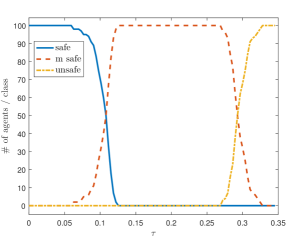
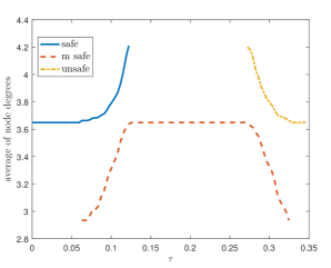
Refer to caption
Refer to caption
Figure 10: The network of Example 2, where τ[0,0.35]𝜏00.35\tau\in[0,0.35].
Example 3.

We consider a network with 100100100 agents and an arbitrary graph topology that satisfies Assumption 1, where the output matrix is incidence matrix of the graph, i.e., C=B100𝐶subscript𝐵100C=B_{100}. The generated network is marginally stable for all time delay τ<0.3415𝜏0.3415\tau<0.3415. The number of observable outputs is 495049504950 and the results of our simulations are illustrated in Figure 11. The effective graph resistance between nodes i𝑖i and j𝑗j,

Ξ𝒢(i,j)=[B100LB100T]ijsubscriptΞ𝒢𝑖𝑗subscriptdelimited-[]subscript𝐵100superscript𝐿superscriptsubscript𝐵100𝑇𝑖𝑗\Xi_{\mathcal{G}}(i,j)=[B_{100}L^{{\dagger}}B_{100}^{T}]_{ij}

is used as a connectivity measure. For two distinct agents, the larger the effective resistance between them, the weaker these agents are connected to each other. Depending on the value of the risk measure with quadratic volatility for each individual event |y¯i|>δisubscript¯𝑦𝑖subscript𝛿𝑖|\overline{y}_{i}|>\delta_{i} for i=1,,4950𝑖14950i=1,\ldots,4950, these events can be labeled as being safe (negative), marginally safe (positive bounded), and unsafe (infinity). The sub-plots in Figure 11 asserts that: for small time delays, the transition from safe mode to marginally safe mode happens between those pair of nodes that maintain a larger than average effective resistance (i.e., lower than average coupling strength), where the average effective resistance is about 0.5440.5440.544. For larger time delay, the transition from marginally safe mode to unsafe mode occurs for those pair of nodes that have a lower than average effective resistance (i.e., higher than average coupling strength).
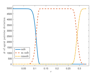
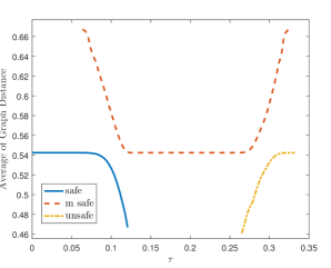
Refer to caption
Refer to caption
Figure 11: The network of Example 3, where τ[0,0.34]𝜏00.34\tau\in[0,0.34].

12 Discussion

There are several points that need to be discussed. The focus of this paper is on the risk of large fluctuations in probability and in expectation. The value of these two types of risk measures capture behavior of relevant microscopic features of a network. Moreover, it turned out that their values depend on network topology through Laplacian spectrum and its eigenvectors. To investigate usefulness of other types of risk measures remains an open problem and is one of our future research directions. The results of this paper are particularly useful to develop design algorithms to optimize network connectivity, performance and risk in presence of external noise and time delay. The design of this class of networks involves only three main scenarios: growing by adding new feedback interconnections, sparsification (eliminating) of existing feedback loops, and reweighing feedback gains. Other design objectives can be obtained by combining these three design procedures. Our particular interest is to design networks that strike a balance among connectivity, performance, and risk. This is one of our current research directions.

A. Delay Differential Equations

Let the initial value problem

φ˙(t)=aφ(tτ),t>0φ(t)=ϕ(t),t[τ,0]\begin{split}\dot{\varphi}(t)&=-a\varphi(t-\tau),\hskip 21.68121ptt>0\\ \varphi(t)&=\phi(t),\hskip 49.14307ptt\in[-\tau,0]\end{split} (43)

where a>0,τ0formulae-sequence𝑎0𝜏0a>0,\leavevmode\nobreak\ \tau\geq 0 and φ=φ(t,0,ϕ),t0formulae-sequence𝜑𝜑𝑡0italic-ϕ𝑡0\varphi=\varphi(t,0,\phi)\in\mathbb{R},\leavevmode\nobreak\ t\geq 0 its solution. It is well-known, [15], that z𝑧z is exponentially stable with respect to zero if and only if aτ<π2.𝑎𝜏𝜋2a\tau<\frac{\pi}{2}. Unfortunately, φ𝜑\varphi attains a closed form expression only when τ=0𝜏0\tau=0, i.e. φ(t)=eatϕ(0)𝜑𝑡superscript𝑒𝑎𝑡italic-ϕ0\varphi(t)=e^{-at}\phi(0). For τ>0𝜏0\tau>0, it is possible to derive a closed form expression of the energy of the fundamental solution of (43); that is the integral 0φ2(t)𝑑tsuperscriptsubscript0superscript𝜑2𝑡differential-d𝑡\int_{0}^{\infty}\varphi^{2}(t)\,dt with φ𝜑\varphi the solution of (43) initiated as ϕ(t)=0italic-ϕ𝑡0\phi(t)=0, t[τ,0)𝑡𝜏0t\in[-\tau,0) and ϕ(0)=1italic-ϕ01\phi(0)=1.

Lemma 3.
777The authors claim no novelty of this result (see for instance [17, 20]). The reason for providing a detailed proof is for the sake of consistency to the formalism of the paper but also because it is derived with alternative and simpler methodology.

If aτ<π2𝑎𝜏𝜋2a\tau<\frac{\pi}{2}, the fundamental solution φ𝜑\varphi of (43) satisfies

0φ2(t)𝑑t=τf(aτ),superscriptsubscript0superscript𝜑2𝑡differential-d𝑡𝜏𝑓𝑎𝜏\int_{0}^{\infty}\varphi^{2}(t)\,dt=\tau f(a\tau),

where f:(0,π2)+:𝑓0𝜋2subscriptf:\big{(}0,\frac{\pi}{2}\big{)}\rightarrow\mathbb{R}_{+} is defined through

f(x)=12xcos(x)1sin(x).𝑓𝑥12𝑥𝑥1𝑥f(x)=\frac{1}{2x}\frac{\cos(x)}{1-\sin(x)}.
Proof.

Given the fundamental solution φ𝜑\varphi, we define the quantity:

V(ρ)=ρφ(t)φ(tρ)𝑑t,ρformulae-sequence𝑉𝜌superscriptsubscript𝜌𝜑𝑡𝜑𝑡𝜌differential-d𝑡𝜌V(\rho)=\int_{\rho}^{\infty}\varphi(t)\varphi(t-\rho)\,dt,\hskip 21.68121pt\rho\in\mathbb{R} (44)
Claim 1.

For V𝑉V as in (44), the following hold:

  1. 1.

    V(ρ)=V(ρ)𝑉𝜌𝑉𝜌V(\rho)=V(-\rho),

  2. 2.

    V˙(ρ)=aV(τρ)˙𝑉𝜌𝑎𝑉𝜏𝜌\dot{V}(\rho)=-aV(\tau-\rho) for ρ>0𝜌0\rho>0, and

  3. 3.

    V(τ)=12a𝑉𝜏12𝑎V(\tau)=\frac{1}{2a}.

Our objective is to calculate V(0)𝑉0V(0). Set R(ρ)=V(τρ)𝑅𝜌𝑉𝜏𝜌R(\rho)=V(\tau-\rho). The pair (V,R)𝑉𝑅(V,R) satisfies the system

V˙=aR,R˙=aV\begin{split}\dot{V}=-aR,\leavevmode\nobreak\ \hskip 28.90755pt\dot{R}=aV\end{split}

where V(0)=R(τ)𝑉0𝑅𝜏V(0)=R(\tau), V(τ)=R(0)=12a𝑉𝜏𝑅012𝑎V(\tau)=R(0)=\frac{1}{2a}, and with solution

(V(ρ)R(ρ))=(cos(aρ)sin(aρ)sin(aρ)cos(aρ))(V(0)R(0)).matrix𝑉𝜌𝑅𝜌matrix𝑎𝜌𝑎𝜌𝑎𝜌𝑎𝜌matrix𝑉0𝑅0\begin{pmatrix}V(\rho)\\ R(\rho)\end{pmatrix}=\begin{pmatrix}\cos(a\rho)&-\sin(a\rho)\\ \sin(a\rho)&\cos(a\rho)\end{pmatrix}\begin{pmatrix}V(0)\\ R(0)\end{pmatrix}.

The second row at ρ=τ𝜌𝜏\rho=\tau reads

R(τ)=sin(aτ)V(0)+cos(aτ)R(0)=V(0).𝑅𝜏𝑎𝜏𝑉0𝑎𝜏𝑅0𝑉0R(\tau)=\sin(a\tau)V(0)+\cos(a\tau)R(0)=V(0).

Solving for V(0)𝑉0V(0), we have

V(0)=cos(aτ)1sin(aτ)R(0)=cos(aτ)1sin(aτ)V(τ),𝑉0𝑎𝜏1𝑎𝜏𝑅0𝑎𝜏1𝑎𝜏𝑉𝜏V(0)=\frac{\cos(a\tau)}{1-\sin(a\tau)}R(0)=\frac{\cos(a\tau)}{1-\sin(a\tau)}V(\tau),

and from (3.)(3.) we conclude

0φ2(t)𝑑t=12acos(aτ)1sin(aτ).superscriptsubscript0superscript𝜑2𝑡differential-d𝑡12𝑎𝑎𝜏1𝑎𝜏\int_{0}^{\infty}\varphi^{2}(t)\,dt=\frac{1}{2a}\frac{\cos(a\tau)}{1-\sin(a\tau)}.

Proof of Claim 1.

For (1.)(1.) we see that

V(ρ)=ρφ(t)φ(t+ρ)𝑑t=0φ(uρ)φ(u)𝑑u=ρφ(uρ)φ(u)𝑑u=V(ρ)𝑉𝜌superscriptsubscript𝜌𝜑𝑡𝜑𝑡𝜌differential-d𝑡superscriptsubscript0𝜑𝑢𝜌𝜑𝑢differential-d𝑢superscriptsubscript𝜌𝜑𝑢𝜌𝜑𝑢differential-d𝑢𝑉𝜌\begin{split}V(-\rho)&=\int_{-\rho}^{\infty}\varphi(t)\varphi(t+\rho)\,dt=\int_{0}^{\infty}\varphi(u-\rho)\varphi(u)\,du\\ &=\int_{\rho}^{\infty}\varphi(u-\rho)\varphi(u)\,du=V(\rho)\end{split}

because φ𝜑\varphi is a fundamental solution. For (2.)(2.) we calculate

ddρV(ρ)=φ(ρ)φ(0)ρφ(t)ρφ(tρ)𝑑t=φ(ρ)+aρφ(t)φ(tρτ)𝑑t=φ(ρ)+aV(ρ+τ).𝑑𝑑𝜌𝑉𝜌𝜑𝜌𝜑0superscriptsubscript𝜌𝜑𝑡𝜌𝜑𝑡𝜌differential-d𝑡𝜑𝜌𝑎superscriptsubscript𝜌𝜑𝑡𝜑𝑡𝜌𝜏differential-d𝑡𝜑𝜌𝑎𝑉𝜌𝜏\begin{split}\frac{d}{d\rho}V(\rho)&=-\varphi(\rho)\varphi(0)-\int_{\rho}^{\infty}\varphi(t)\frac{\partial}{\partial\rho}\varphi(t-\rho)\,dt\\ &=-\varphi(\rho)+a\int_{\rho}^{\infty}\varphi(t)\varphi(t-\rho-\tau)\,dt\\ &=-\varphi(\rho)+aV(\rho+\tau).\end{split} (45)

From the symmetry of V𝑉V,

ddρV(ρ)=ddρ[V(ρ)]=ddρV(ρ)=φ(ρ)aV(ρ+τ)=aV(τρ)𝑑𝑑𝜌𝑉𝜌𝑑𝑑𝜌delimited-[]𝑉𝜌𝑑𝑑𝜌𝑉𝜌𝜑𝜌𝑎𝑉𝜌𝜏𝑎𝑉𝜏𝜌\begin{split}\frac{d}{d\rho}V(\rho)&=\frac{d}{d\rho}\big{[}V(-\rho)\big{]}=-\frac{d}{d\rho}V(-\rho)\\ &=-\varphi(-\rho)-aV(-\rho+\tau)=-aV(\tau-\rho)\end{split}

so long as ρ>0𝜌0\rho>0. Finally, while (45) yields

V˙(0)=φ(0)+aV(τ)=1+aV(τ),˙𝑉0𝜑0𝑎𝑉𝜏1𝑎𝑉𝜏\dot{V}(0)=-\varphi(0)+aV(\tau)=-1+aV(\tau),

from property (2.)(2.) we obtain V˙(0)=aV(τ).˙𝑉0𝑎𝑉𝜏\dot{V}(0)=-aV(\tau). The result occurs after equating the right hand sides of these two expressions. ∎

B. Proofs Of Technical Results

Proof of Lemma 1.

Direct calculations yield

CΣtC=0tCQΦ(ts)QTBBTQΦ(ts)QTC𝑑s=b2CQ0tΦ2(ts)𝑑s(CQ)T,𝐶subscriptΣ𝑡𝐶superscriptsubscript0𝑡𝐶𝑄Φ𝑡𝑠superscript𝑄𝑇𝐵superscript𝐵𝑇𝑄Φ𝑡𝑠superscript𝑄𝑇𝐶differential-d𝑠superscript𝑏2𝐶𝑄superscriptsubscript0𝑡superscriptΦ2𝑡𝑠differential-d𝑠superscript𝐶𝑄𝑇\begin{split}C\Sigma_{t}C&=\int_{0}^{t}CQ\Phi(t-s)Q^{T}BB^{T}Q\Phi(t-s)\hskip 1.42271ptQ^{T}C\,ds\\ &=b^{2}\hskip 1.42271ptCQ\int_{0}^{t}\Phi^{2}(t-s)\,ds\leavevmode\nobreak\ (CQ)^{T},\end{split}

where ΦL(t)=QΦ(t)QTsubscriptΦ𝐿𝑡𝑄Φ𝑡superscript𝑄𝑇\Phi_{L}(t)=Q\Phi(t)Q^{T} in which Φ(t)=diag(φ1(t),,φn(t))Φ𝑡diagsubscript𝜑1𝑡subscript𝜑𝑛𝑡\Phi(t)=\mathrm{diag}\big{(}\varphi_{1}(t),\ldots,\varphi_{n}(t)\big{)} and φksubscript𝜑𝑘\varphi_{k}’s are eigensolutions of the unperturbed network. By letting C=[𝐜1,,𝐜N]T𝐶superscriptsubscript𝐜1subscript𝐜𝑁𝑇C=[\mathbf{c}_{1},\dots,\mathbf{c}_{N}]^{T}, the elements of CΣtCT𝐶subscriptΣ𝑡superscript𝐶𝑇C\Sigma_{t}C^{T} are given by

[CΣtCT]ij=b2[0tk(𝐜iT𝐪k)φk2(ts)(𝐜jT𝐪k)ds]ij.subscriptdelimited-[]𝐶subscriptΣ𝑡superscript𝐶𝑇𝑖𝑗superscript𝑏2subscriptdelimited-[]superscriptsubscript0𝑡subscript𝑘superscriptsubscript𝐜𝑖𝑇subscript𝐪𝑘superscriptsubscript𝜑𝑘2𝑡𝑠superscriptsubscript𝐜𝑗𝑇subscript𝐪𝑘𝑑𝑠𝑖𝑗\begin{split}&[C\Sigma_{t}C^{T}]_{ij}=b^{2}\bigg{[}\int_{0}^{t}\sum_{k}(\mathbf{c}_{i}^{T}\mathbf{q}_{k})\varphi_{k}^{2}(t-s)(\mathbf{c}_{j}^{T}\mathbf{q}_{k})\,ds\bigg{]}_{ij}.\end{split}

According to our assumptions, it follows that φ1(t)1subscript𝜑1𝑡1\varphi_{1}(t)\equiv 1 and all φk(t)subscript𝜑𝑘𝑡\varphi_{k}(t) for k=2,,n𝑘2𝑛k=2,\ldots,n are exponentially fast vanishing functions. Therefore, matrix CΣtC𝐶subscriptΣ𝑡𝐶C\Sigma_{t}C is bounded if and only if k(𝐜iT𝐪1)(𝐜jT𝐪1)=0subscript𝑘superscriptsubscript𝐜𝑖𝑇subscript𝐪1superscriptsubscript𝐜𝑗𝑇subscript𝐪10\sum_{k}(\mathbf{c}_{i}^{T}\mathbf{q}_{1})(\mathbf{c}_{j}^{T}\mathbf{q}_{1})=0 for all i,j𝒱𝑖𝑗𝒱i,j\in{\mathcal{V}}. But for i=j𝑖𝑗i=j we have (𝐜iT𝐪1)2=0superscriptsuperscriptsubscript𝐜𝑖𝑇subscript𝐪120(\mathbf{c}_{i}^{T}\mathbf{q}_{1})^{2}=0 for all i𝑖i. The reverse part is trivial. ∎

Proof of Proposition 1.

(i.) If z𝑧z is independent of ωΩ𝜔Ω\omega\in\Omega, then (z>δ)=0𝑧𝛿0\mathbb{P}(z>\delta)=0 for any δ𝛿\delta arbitrarily close to z𝑧z from the right. In view of ε[0,1)𝜀01\varepsilon\in[0,1), the definition of ε(z)subscript𝜀𝑧\mathcal{R}_{\varepsilon}(z) imposes the infimum of the sum that is achieved when all δ𝛿\delta attain the infimum value which is z𝑧z.

(ii.) Note that ε(z+m)=inf{δ|(z(ω)+m>δ)<ε}subscript𝜀𝑧𝑚infimumconditional-set𝛿𝑧𝜔𝑚𝛿𝜀\mathcal{R}_{\varepsilon}(z+m)=\inf\{\delta\leavevmode\nobreak\ |\leavevmode\nobreak\ \mathbb{P}\big{(}z(\omega)+m>\delta\big{)}<\varepsilon\} is equivalent to inf{δ|(z(ω)>δm)<ε}infimumconditional-set𝛿𝑧𝜔𝛿𝑚𝜀\inf\{\delta\leavevmode\nobreak\ |\leavevmode\nobreak\ \mathbb{P}\big{(}z(\omega)>\delta-m\big{)}<\varepsilon\}. For δ:=δ+massignsuperscript𝛿𝛿𝑚\delta^{\prime}:=\delta+m we obtain ε(z+m)=inf{δ+m|(z(ω)>δ)<ε}=m+inf{δ|(z(ω)>δ)<ε}=ε(z)subscript𝜀𝑧𝑚infimumconditional-setsuperscript𝛿𝑚𝑧𝜔superscript𝛿𝜀𝑚infimumconditional-setsuperscript𝛿𝑧𝜔superscript𝛿𝜀subscript𝜀𝑧\mathcal{R}_{\varepsilon}(z+m)=\inf\{\delta^{\prime}+m\leavevmode\nobreak\ |\leavevmode\nobreak\ \mathbb{P}\big{(}z(\omega)>\delta^{\prime}\big{)}<\varepsilon\}=m+\inf\{\delta^{\prime}\leavevmode\nobreak\ |\leavevmode\nobreak\ \mathbb{P}\big{(}z(\omega)>\delta^{\prime}\big{)}<\varepsilon\}=\mathcal{R}_{\varepsilon}(z).

(iii.) Let z1,z2𝕃2subscript𝑧1subscript𝑧2superscript𝕃2z_{1},z_{2}\in\mathbb{L}^{2} with z1z2subscript𝑧1subscript𝑧2z_{1}\leq z_{2} almost surely. Then {z1>δ}{z2>δ}subscript𝑧1𝛿subscript𝑧2𝛿\{z_{1}>\delta\}\subseteq\{z_{2}>\delta\} that implies (z1>δ)(z2>δ)subscript𝑧1𝛿subscript𝑧2𝛿\mathbb{P}\big{(}z_{1}>\delta\big{)}\leq\mathbb{P}\big{(}z_{2}>\delta\big{)}. The decrease of δ𝛿\delta on z1subscript𝑧1z_{1} to achieve ε𝜀\varepsilon is smaller than the corresponding decrease on z2subscript𝑧2z_{2}. So the risk of z1subscript𝑧1z_{1} cannot be larger than the risk of z2subscript𝑧2z_{2}.

(iv.) For any λ>0𝜆0\lambda>0, (λy>δ)=(y>δ/λ)𝜆𝑦𝛿𝑦𝛿𝜆\mathbb{P}\big{(}\lambda y>\delta\big{)}=\mathbb{P}\big{(}y>\delta/\lambda\big{)} and simple substitutions yield the result.

(v.) Let z=αx+(1α)y𝑧𝛼𝑥1𝛼𝑦z=\alpha x+(1-\alpha)y with x,y𝕃2𝑥𝑦superscript𝕃2x,y\in\mathbb{L}^{2} and (xy)=p𝑥𝑦𝑝\mathbb{P}\big{(}x\leq y\big{)}=p, (x>y)=1p𝑥𝑦1𝑝\mathbb{P}\big{(}x>y\big{)}=1-p and α[0,1]𝛼01\alpha\in[0,1]. Then

(z>δ)=(z>δ|xy)p+(z>δ|x>y)(1p).𝑧𝛿𝑧conditional𝛿𝑥𝑦𝑝𝑧𝛿ket𝑥𝑦1𝑝\mathbb{P}\big{(}z>\delta\big{)}=\mathbb{P}\big{(}z>\delta|x\leq y\big{)}p+\mathbb{P}\big{(}z>\delta|x>y\big{)}(1-p).

If xy𝑥𝑦x\leq y, then (z>δ)(y>δ)𝑧𝛿𝑦𝛿\mathbb{P}\big{(}z>\delta\big{)}\leq\mathbb{P}(y>\delta\big{)} while, if xy𝑥𝑦x\geq y, then (z>δ)(x>δ)𝑧𝛿𝑥𝛿\mathbb{P}\big{(}z>\delta\big{)}\leq\mathbb{P}(x>\delta\big{)} Using the last two inequalities and property (iii.)(iii.) the result follows. ∎

Proof of Proposition 2.

(i.) Follows similarly with (ii.)(ii.) of Proposition 1.

(ii.) Due to the convexity and monotonicity properties of v𝑣v, it is easy to verify that 𝔸𝔸\mathbb{A} is convex. Now let {zi}i=1,2𝔸subscriptsubscript𝑧𝑖𝑖12𝔸\{z_{i}\}_{i=1,2}\in\mathbb{A} and {δi}i=1,20subscriptsubscript𝛿𝑖𝑖120\{\delta_{i}\}_{i=1,2}\leq 0 the corresponding risk values. In view of (i.)(i.), it holds that 𝒯ε(ziδi)=0subscript𝒯𝜀subscript𝑧𝑖subscript𝛿𝑖0\mathcal{T}_{\varepsilon}(z_{i}-\delta_{i})=0, i.e. ziδi𝔸subscript𝑧𝑖subscript𝛿𝑖𝔸z_{i}-\delta_{i}\in\mathbb{A} and by convexity

α(z1δ1)+(1α)(z2δ2)𝔸.𝛼subscript𝑧1subscript𝛿11𝛼subscript𝑧2subscript𝛿2𝔸\alpha(z_{1}-\delta_{1})+(1-\alpha)(z_{2}-\delta_{2})\in\mathbb{A}.

Again from (i.)(i.) we get

0𝒯ε(α(z1δ1)+(1α)(z2δ2))=𝒯ε((αz1+(1α)z2)(αδ1+(1α)δ2)).0subscript𝒯𝜀𝛼subscript𝑧1subscript𝛿11𝛼subscript𝑧2subscript𝛿2subscript𝒯𝜀𝛼subscript𝑧11𝛼subscript𝑧2𝛼subscript𝛿11𝛼subscript𝛿2\begin{split}0&\geq\mathcal{T}_{\varepsilon}\big{(}\alpha(z_{1}-\delta_{1})+(1-\alpha)(z_{2}-\delta_{2})\big{)}\\ &=\mathcal{T}_{\varepsilon}\big{(}(\alpha z_{1}+(1-\alpha)z_{2})-(\alpha\delta_{1}+(1-\alpha)\delta_{2})\big{)}.\end{split}

which yields the result.

(iii.) If z2z1subscript𝑧2subscript𝑧1z_{2}\leq z_{1} then z2δz1δsubscript𝑧2𝛿subscript𝑧1𝛿z_{2}-\delta\leq z_{1}-\delta, so that z2δz1δsubscript𝑧2𝛿subscript𝑧1𝛿z_{2}-\delta\leq z_{1}-\delta and v(z2δ)u(z1δ)𝑣subscript𝑧2𝛿𝑢subscript𝑧1𝛿v(z_{2}-\delta)\leq u(z_{1}-\delta). Consequently the cost δ𝛿\delta to bring v(z2δ)𝑣subscript𝑧2𝛿v(z_{2}-\delta) closer to v(ε)𝑣𝜀v(\varepsilon) is smaller than the respective cost on u(z1δ)𝑢subscript𝑧1𝛿u(z_{1}-\delta).

(iv.) For every z𝔹𝑧𝔹z\in\mathbb{B}, (iii.) shows that λz𝔸𝜆𝑧𝔸\lambda z\in\mathbb{A} as well for λ0𝜆0\lambda\geq 0. We take cases on λ𝜆\lambda:

λ[0,1]𝜆01\lambda\in[0,1] : Then λz+𝟏(1λ)ε𝔸𝜆𝑧11𝜆𝜀𝔸\lambda z+\mathbf{1}(1-\lambda)\varepsilon\in\mathbb{A} as one can verify that 𝒯ε(𝟏ε)=0subscript𝒯𝜀1𝜀0\mathcal{T}_{\varepsilon}(\mathbf{1}\varepsilon)=0, i.e. ε𝔸𝜀𝔸\varepsilon\in\mathbb{A}. From (i.), 𝒯ε(λz)+(1λ)ε=𝒯ε(λz+(1λ)𝟏ε)λ𝒯ε(z)subscript𝒯𝜀𝜆𝑧1𝜆𝜀subscript𝒯𝜀𝜆𝑧1𝜆1𝜀𝜆subscript𝒯𝜀𝑧\mathcal{T}_{\varepsilon}(\lambda z)+(1-\lambda)\varepsilon=\mathcal{T}_{\varepsilon}(\lambda z+(1-\lambda)\mathbf{1}\varepsilon)\leq\lambda\mathcal{T}_{\varepsilon}(z), and solving for 𝒯ε(λz)subscript𝒯𝜀𝜆𝑧\mathcal{T}_{\varepsilon}(\lambda z) we obtain the result.

λ1𝜆1\lambda\geq 1 : Then it follows from λz,𝟏ε𝔸𝜆𝑧1𝜀𝔸\lambda z,\mathbf{1}\varepsilon\in\mathbb{A} and properties (i.) and (ii.): 𝒯ε(z)+(1λ1)ε=𝒯ε(z+(1λ1)ε)=𝒯ε(λ1(λz)+(1λ1)ε)λ1𝒯ε(λz)subscript𝒯𝜀𝑧1superscript𝜆1𝜀subscript𝒯𝜀𝑧1superscript𝜆1𝜀subscript𝒯𝜀superscript𝜆1𝜆𝑧1superscript𝜆1𝜀superscript𝜆1subscript𝒯𝜀𝜆𝑧\mathcal{T}_{\varepsilon}(z)+(1-\lambda^{-1})\varepsilon=\mathcal{T}_{\varepsilon}(z+(1-\lambda^{-1})\varepsilon)=\mathcal{T}_{\varepsilon}(\lambda^{-1}(\lambda z)+(1-\lambda^{-1})\varepsilon)\leq\lambda^{-1}\mathcal{T}_{\varepsilon}(\lambda z). Solving for 𝒯ε(λz)subscript𝒯𝜀𝜆𝑧\mathcal{T}_{\varepsilon}(\lambda z) we obtain the result. ∎

Proof of Lemma 2.

We write σt2(Q)=b2𝐜TQ0tΦ2(ts)𝑑sQT𝐜superscriptsubscript𝜎𝑡2𝑄superscript𝑏2superscript𝐜𝑇𝑄superscriptsubscript0𝑡superscriptΦ2𝑡𝑠differential-d𝑠superscript𝑄𝑇𝐜\sigma_{t}^{2}(Q)=b^{2}\mathbf{c}^{T}Q\int_{0}^{t}\Phi^{2}(t-s)\,dsQ^{T}\mathbf{c} and with little abuse of notation our focus is on the matrix Σt=b2Q0tΦ2(ts)𝑑sQTsubscriptΣ𝑡superscript𝑏2𝑄superscriptsubscript0𝑡superscriptΦ2𝑡𝑠differential-d𝑠superscript𝑄𝑇\Sigma_{t}=b^{2}Q\int_{0}^{t}\Phi^{2}(t-s)\,ds\,Q^{T} . This is a diagonal form for every t𝑡t and characterizes the algebraic multiplicity of the eigenvalues ζk=ζk(t)=0tφk2(ts)𝑑s,i𝒱formulae-sequencesubscript𝜁𝑘subscript𝜁𝑘𝑡superscriptsubscript0𝑡superscriptsubscript𝜑𝑘2𝑡𝑠differential-d𝑠𝑖𝒱\zeta_{k}=\zeta_{k}(t)=\int_{0}^{t}\varphi_{k}^{2}(t-s)\,ds,\leavevmode\nobreak\ i\in{\mathcal{V}}. Fix t𝑡t and i𝒱𝑖𝒱i\in{\mathcal{V}}. Note that we can write σt2(Q)=b2kζk(t)j=1mi(cjQ)2superscriptsubscript𝜎𝑡2𝑄superscript𝑏2subscript𝑘subscript𝜁𝑘𝑡superscriptsubscript𝑗1subscript𝑚𝑖superscriptsuperscriptsubscript𝑐𝑗𝑄2\sigma_{t}^{2}(Q)=b^{2}\sum_{k}\zeta_{k}(t)\sum_{j=1}^{m_{i}}(c_{j}^{Q})^{2} where mk=mk(t)subscript𝑚𝑘subscript𝑚𝑘𝑡m_{k}=m_{k}(t) is the algebraic multiplicity of ζksubscript𝜁𝑘\zeta_{k}. We take cases.

mk=1subscript𝑚𝑘1m_{k}=1: the corresponding normal (real) eigenvector is unique up to a sign. Consequently, ckQ1=±ckQ2superscriptsubscript𝑐𝑘subscript𝑄1plus-or-minussuperscriptsubscript𝑐𝑘subscript𝑄2c_{k}^{Q_{1}}=\pm c_{k}^{Q_{2}} therefore (ckQ1)2=(ckQ2)2superscriptsuperscriptsubscript𝑐𝑘subscript𝑄12superscriptsuperscriptsubscript𝑐𝑘subscript𝑄22(c_{k}^{Q_{1}})^{2}=(c_{k}^{Q_{2}})^{2}.

mk>1subscript𝑚𝑘1m_{k}>1: ζk(t)subscript𝜁𝑘𝑡\zeta_{k}(t) is repeated mksubscript𝑚𝑘m_{k} times while it produces mksubscript𝑚𝑘m_{k} linearly independent normal eigenvectors that can be chosen mutually orthogonal. Then the collection of the eigenvectors of Q1subscript𝑄1Q_{1} that span the subspace of ζk(t)subscript𝜁𝑘𝑡\zeta_{k}(t), say Q1ζksubscriptsuperscript𝑄subscript𝜁𝑘1Q^{\zeta_{k}}_{1} and the corresponding collection of Q2ζksubscriptsuperscript𝑄subscript𝜁𝑘2Q^{\zeta_{k}}_{2} of Q2subscript𝑄2Q_{2} are associated with an orthogonal matrix P𝑃P such that Q1ζk=Q2ζkPsuperscriptsubscript𝑄1subscript𝜁𝑘superscriptsubscript𝑄2subscript𝜁𝑘𝑃Q_{1}^{\zeta_{k}}=Q_{2}^{\zeta_{k}}P. Then

j=1mi(cjQ1ζk)2=𝐜TQ1ζk(𝐜TQ1ζk)T=𝐜TQ2ζkP(𝐜TQ2ζkP)T=𝐜TQ2ζkPPT(Q2ζk)T𝐜=𝐜TQ2ζk(𝐜TQ2ζk)T=j=1mi(cjQ2ζk)2.superscriptsubscript𝑗1subscript𝑚𝑖superscriptsuperscriptsubscript𝑐𝑗superscriptsubscript𝑄1subscript𝜁𝑘2superscript𝐜𝑇superscriptsubscript𝑄1subscript𝜁𝑘superscriptsuperscript𝐜𝑇superscriptsubscript𝑄1subscript𝜁𝑘𝑇superscript𝐜𝑇superscriptsubscript𝑄2subscript𝜁𝑘𝑃superscriptsuperscript𝐜𝑇superscriptsubscript𝑄2subscript𝜁𝑘𝑃𝑇superscript𝐜𝑇superscriptsubscript𝑄2subscript𝜁𝑘𝑃superscript𝑃𝑇superscriptsuperscriptsubscript𝑄2subscript𝜁𝑘𝑇𝐜superscript𝐜𝑇superscriptsubscript𝑄2subscript𝜁𝑘superscriptsuperscript𝐜𝑇superscriptsubscript𝑄2subscript𝜁𝑘𝑇superscriptsubscript𝑗1subscript𝑚𝑖superscriptsuperscriptsubscript𝑐𝑗superscriptsubscript𝑄2subscript𝜁𝑘2\begin{split}&\sum_{j=1}^{m_{i}}(c_{j}^{Q_{1}^{\zeta_{k}}})^{2}=\mathbf{c}^{T}Q_{1}^{\zeta_{k}}(\mathbf{c}^{T}Q_{1}^{\zeta_{k}})^{T}=\mathbf{c}^{T}Q_{2}^{\zeta_{k}}P(\mathbf{c}^{T}Q_{2}^{\zeta_{k}}P)^{T}\\ &=\mathbf{c}^{T}Q_{2}^{\zeta_{k}}PP^{T}(Q_{2}^{\zeta_{k}})^{T}\mathbf{c}=\mathbf{c}^{T}Q_{2}^{\zeta_{k}}(\mathbf{c}^{T}Q_{2}^{\zeta_{k}})^{T}=\sum_{j=1}^{m_{i}}(c_{j}^{Q_{2}^{\zeta_{k}}})^{2}.\end{split}

For t𝑡t and k𝑘k being arbitrary, the result follows. ∎

Proof of Theorem 1.

From the discussion in §6, yt𝒩(μt,σt2)similar-tosubscript𝑦𝑡𝒩subscript𝜇𝑡superscriptsubscript𝜎𝑡2y_{t}\sim\mathcal{N}(\mu_{t},\sigma_{t}^{2}) with μtsubscript𝜇𝑡\mu_{t} and σt2superscriptsubscript𝜎𝑡2\sigma_{t}^{2} as in (15) and (16). Then |yt|subscript𝑦𝑡|y_{t}| follows a folded normal distribution with mean μ|yt|subscript𝜇subscript𝑦𝑡\mu_{|y_{t}|} and variance σ|yt|2superscriptsubscript𝜎subscript𝑦𝑡2\sigma_{|y_{t}|}^{2} defined in the statement of the theorem. For the volatility risks we distinguish between v(x)=x2𝑣𝑥superscript𝑥2v(x)=x^{2} and v(x)=eβx𝑣𝑥superscript𝑒𝛽𝑥v(x)=e^{\beta x}.

For v(x)=x2𝑣𝑥superscript𝑥2v(x)=x^{2}, 𝒯ε(|yt|)=inf{δ:𝔼[(|yt|δ)2]ε2}subscript𝒯𝜀subscript𝑦𝑡infimumconditional-set𝛿𝔼delimited-[]superscriptsubscript𝑦𝑡𝛿2superscript𝜀2\mathcal{T}_{\varepsilon}(|y_{t}|)=\inf\big{\{}\delta\in\mathbb{R}:\mathbb{E}[(|y_{t}|-\delta)^{2}]\leq\varepsilon^{2}\big{\}} Solving for δ𝛿\delta the inequality 𝔼[(|yt|δ)2]ε2𝔼delimited-[]superscriptsubscript𝑦𝑡𝛿2superscript𝜀2\mathbb{E}[(|y_{t}|-\delta)^{2}]\leq\varepsilon^{2} we obtain that the infimum is achieved at the root δ=𝔼[|yt|]ε2𝔼[(|yt|𝔼[|yt|])2]𝛿𝔼delimited-[]subscript𝑦𝑡superscript𝜀2𝔼delimited-[]superscriptsubscript𝑦𝑡𝔼delimited-[]subscript𝑦𝑡2\delta=\mathbb{E}[|y_{t}|]-\sqrt{\varepsilon^{2}-\mathbb{E}\big{[}\big{(}|y_{t}|-\mathbb{E}[|y_{t}|]\big{)}^{2}\big{]}}. For v(x)=eβx𝑣𝑥superscript𝑒𝛽𝑥v(x)=e^{\beta x},

𝔼[eβ(|yt|δ)]eβεδ1βln(𝔼[eβ(|yt|ε)])𝔼delimited-[]superscript𝑒𝛽subscript𝑦𝑡𝛿superscript𝑒𝛽𝜀𝛿1𝛽𝔼delimited-[]superscript𝑒𝛽subscript𝑦𝑡𝜀\mathbb{E}\big{[}e^{\beta(|y_{t}|-\delta)}\big{]}\leq e^{\beta\varepsilon}\Leftrightarrow\delta\geq\frac{1}{\beta}\ln\big{(}\mathbb{E}[e^{\beta(|y_{t}|-\varepsilon)}]\big{)}

so 𝒯ε(|yt|)=1βln(𝔼[eβ(|yt|ε)])subscript𝒯𝜀subscript𝑦𝑡1𝛽𝔼delimited-[]superscript𝑒𝛽subscript𝑦𝑡𝜀\mathcal{T}_{\varepsilon}(|y_{t}|)=\frac{1}{\beta}\ln\big{(}\mathbb{E}[e^{\beta(|y_{t}|-\varepsilon)}]\big{)} and the result follows by straightforward algebra on

𝔼[eβ|yt|]=eβ|u|e(uμt)22σt2𝑑u.𝔼delimited-[]superscript𝑒𝛽subscript𝑦𝑡superscriptsubscriptsuperscript𝑒𝛽𝑢superscript𝑒superscript𝑢subscript𝜇𝑡22superscriptsubscript𝜎𝑡2differential-d𝑢\mathbb{E}[e^{\beta|y_{t}|}]=\int_{-\infty}^{\infty}e^{\beta|u|}e^{-\frac{(u-\mu_{t})^{2}}{2\sigma_{t}^{2}}}\,du.

Finaly from Eq. (3) we calculate the probability

ε(|yt|)=inf{δ>0:(|yt|>δ)ε}=inf{δ>0:(|yt|δ)1ε}=inf{δ>0:12πσtδδe(xμt)22σt2𝑑x(1ε)}=inf{2σtδ+μt>0:1πδ2μt2σtδeu2𝑑u(1ε)}=2σtSε(μt2σt)+μt,subscript𝜀subscript𝑦𝑡infimumconditional-set𝛿0subscript𝑦𝑡𝛿𝜀infimumconditional-set𝛿0subscript𝑦𝑡𝛿1𝜀infimumconditional-set𝛿012𝜋subscript𝜎𝑡superscriptsubscript𝛿𝛿superscript𝑒superscript𝑥subscript𝜇𝑡22superscriptsubscript𝜎𝑡2differential-d𝑥1𝜀infimumconditional-set2subscript𝜎𝑡𝛿subscript𝜇𝑡01𝜋superscriptsubscript𝛿2subscript𝜇𝑡2subscript𝜎𝑡𝛿superscript𝑒superscript𝑢2differential-d𝑢1𝜀2subscript𝜎𝑡subscript𝑆𝜀subscript𝜇𝑡2subscript𝜎𝑡subscript𝜇𝑡\begin{split}&\mathcal{R}_{\varepsilon}\big{(}|y_{t}|\big{)}=\inf\big{\{}\delta>0:\mathbb{P}(|y_{t}|>\delta)\leq\varepsilon\big{\}}\\ &=\inf\big{\{}\delta>0:\mathbb{P}(|y_{t}|\leq\delta)\geq 1-\varepsilon\big{\}}\\ &=\inf\bigg{\{}\delta>0:\frac{1}{\sqrt{2\pi}\sigma_{t}}\int_{-\delta}^{\delta}e^{-\frac{(x-\mu_{t})^{2}}{2\sigma_{t}^{2}}}\,dx\geq(1-\varepsilon)\bigg{\}}\\ &=\inf\bigg{\{}\sqrt{2}\sigma_{t}\delta+\mu_{t}>0:\frac{1}{\sqrt{\pi}}\int_{-\delta-2\frac{\mu_{t}}{\sqrt{2}\sigma_{t}}}^{\delta}e^{-u^{2}}\,du\geq(1-\varepsilon)\bigg{\}}\\ &=\sqrt{2}\sigma_{t}S_{\varepsilon}\bigg{(}\frac{\mu_{t}}{\sqrt{2}\sigma_{t}}\bigg{)}+\mu_{t},\end{split}

where Sε(α)subscript𝑆𝜀𝛼S_{\varepsilon}(\alpha) as in (3). ∎

Proof of Theorem 2.

The condition 𝐜T𝐪1=0superscript𝐜𝑇subscript𝐪10\mathbf{c}^{T}\mathbf{q}_{1}=0 implies c1Q=0superscriptsubscript𝑐1𝑄0c_{1}^{Q}=0 or equivalently the marginally stable mode to be unobservable at the output. This implies limt+μt=0subscript𝑡subscript𝜇𝑡0\lim_{t\rightarrow+\infty}\mu_{t}=0 for μtsubscript𝜇𝑡\mu_{t} as in (15) and limt+μ|yt|=2πσ¯subscript𝑡subscript𝜇subscript𝑦𝑡2𝜋¯𝜎\lim_{t\rightarrow+\infty}\mu_{|y_{t}|}=\sqrt{\frac{2}{\pi}}\overline{\sigma} for σ¯=limt+σt¯𝜎subscript𝑡subscript𝜎𝑡\overline{\sigma}=\lim_{t\rightarrow+\infty}\sigma_{t} and σtsubscript𝜎𝑡\sigma_{t} as in (16). Of course, σ¯2=k>1(ckQ)20φk2(s)𝑑ssuperscript¯𝜎2subscript𝑘1superscriptsuperscriptsubscript𝑐𝑘𝑄2superscriptsubscript0superscriptsubscript𝜑𝑘2𝑠differential-d𝑠\overline{\sigma}^{2}=\sum_{k>1}(c_{k}^{Q})^{2}\int_{0}^{\infty}\varphi_{k}^{2}(s)\,ds and we can combine Theorem 1 together with Lemma 7 to derive the corresponding expressions (22), (23) and (20) for all three risk measures. ∎

Proof of Theorem 3.

Direct calculations, yield

τσ¯2=12b2k=2n11sin(λkτ)(ckQ)2>0.𝜏superscript¯𝜎212superscript𝑏2superscriptsubscript𝑘2𝑛11subscript𝜆𝑘𝜏superscriptsuperscriptsubscript𝑐𝑘𝑄20\frac{\partial}{\partial\tau}\overline{\sigma}^{2}=\frac{1}{2}b^{2}\sum_{k=2}^{n}\frac{1}{1-\sin(\lambda_{k}\tau)}(c_{k}^{Q})^{2}>0.

From this and the fact the systemic risk measures are increasing functions of σ¯¯𝜎\overline{\sigma}, it immediately follows that εsubscript𝜀\mathcal{R}_{\varepsilon} or 𝒯εsubscript𝒯𝜀\mathcal{T}_{\varepsilon} are strictly increasing functions of time delay as well. ∎

Proof of Theorem 4.

We observe that 𝓡ε(|𝐲¯|)subscript𝓡𝜀¯𝐲\boldsymbol{\mathcal{R}}_{\varepsilon}(|\overline{\mathbf{y}}|) is a set-valued function whose value is equivalent to the solution of the following multi-dimensional joint chance-constrained optimization problem

minimize𝜹𝜹𝜹minimize𝜹\displaystyle\underset{\boldsymbol{\delta}}{\textrm{minimize}}\leavevmode\nobreak\ \leavevmode\nobreak\ \boldsymbol{\delta} (46)
subject to:(|𝐲¯|𝜹)1ε.subject to:precedes-or-equals¯𝐲𝜹1𝜀\displaystyle\mbox{subject to:}\leavevmode\nobreak\ \leavevmode\nobreak\ \mathbb{P}\left(\hskip 1.42271pt|\overline{\mathbf{y}}|\preceq\boldsymbol{\delta}\hskip 1.42271pt\right)\geq 1-\varepsilon. (47)

In general, this problem is very difficult to solve even numerically, let alone find closed form solutions. To overcome computational complexity and calculate bounds, we decompose the joint probability constraint (47) into several individual constraints. Let us consider positive numbers ε1,,εqsubscript𝜀1subscript𝜀𝑞\varepsilon_{1},\ldots,\varepsilon_{q} such that (30) holds. Suppose that δksuperscriptsubscript𝛿𝑘\delta_{k}^{*} is the optimal solution of the following optimization problem

minimizeδkδksubscript𝛿𝑘minimizesubscript𝛿𝑘\displaystyle\underset{\delta_{k}}{\textrm{minimize}}\leavevmode\nobreak\ \leavevmode\nobreak\ \delta_{k} (48)
subject to:(|y¯k|δk)1εksubject to:subscript¯𝑦𝑘subscript𝛿𝑘1subscript𝜀𝑘\displaystyle\mbox{subject to:}\leavevmode\nobreak\ \leavevmode\nobreak\ \mathbb{P}\left(\hskip 1.42271pt|\overline{y}_{k}|\leq\delta_{k}\hskip 1.42271pt\right)\geq 1-\varepsilon_{k} (49)

for k=1,,q𝑘1𝑞k=1,\ldots,q. is an upper bound for the optimal solution of (46)-(47). Let us denote 𝜹=[δ1,,δq]Tsuperscript𝜹superscriptsuperscriptsubscript𝛿1superscriptsubscript𝛿𝑞𝑇\boldsymbol{\delta}^{*}=[\delta_{1}^{*},\ldots,\delta_{q}^{*}]^{T}. From Bonferroni inequality [12], we have that

(|𝐲¯|𝜹)k=1q(|y¯k|δk)(q1)precedes-or-equals¯𝐲superscript𝜹superscriptsubscript𝑘1𝑞subscript¯𝑦𝑘superscriptsubscript𝛿𝑘𝑞1\mathbb{P}\left(\hskip 1.42271pt|\overline{\mathbf{y}}|\preceq\boldsymbol{\delta}^{*}\hskip 1.42271pt\right)\leavevmode\nobreak\ \geq\leavevmode\nobreak\ \sum_{k=1}^{q}\mathbb{P}\left(\hskip 1.42271pt|\overline{y}_{k}|\leq\delta_{k}^{*}\hskip 1.42271pt\right)-(q-1)

From constraint (30) and (49), it follows that

(|𝐲¯|𝜹)precedes-or-equals¯𝐲superscript𝜹\displaystyle\mathbb{P}\left(\hskip 1.42271pt|\overline{\mathbf{y}}|\preceq\boldsymbol{\delta}^{*}\hskip 1.42271pt\right) \displaystyle\geq k=1q(1εk)(q1)=1k=1qεk 1ε.superscriptsubscript𝑘1𝑞1subscript𝜀𝑘𝑞11superscriptsubscript𝑘1𝑞subscript𝜀𝑘1𝜀\displaystyle\sum_{k=1}^{q}(1-\varepsilon_{k})-(q-1)=1-\sum_{k=1}^{q}\varepsilon_{k}\leavevmode\nobreak\ \geq\leavevmode\nobreak\ 1-\varepsilon.

This implies that 𝜹superscript𝜹\boldsymbol{\delta}^{*} is a feasible solution for optimization problem (46)-(47). Thus, we conclude that

𝓡ε(|𝐲¯|)subscript𝓡𝜀¯𝐲\displaystyle\boldsymbol{\mathcal{R}}_{\varepsilon}(|\overline{\mathbf{y}}|) precedes-or-equals\displaystyle\preceq [δ1,,δq]T[ε1(|y¯1|),,εq(|y¯q|)]T.precedes-or-equalssuperscriptsuperscriptsubscript𝛿1superscriptsubscript𝛿𝑞𝑇superscriptsubscriptsubscript𝜀1subscript¯𝑦1subscriptsubscript𝜀𝑞subscript¯𝑦𝑞𝑇\displaystyle[\hskip 1.42271pt\delta_{1}^{*},\ldots,\delta_{q}^{*}\hskip 1.42271pt]^{T}\preceq\left[\hskip 1.42271pt{\mathcal{R}}_{\varepsilon_{1}}(|\overline{y}_{1}|),\leavevmode\nobreak\ \ldots\leavevmode\nobreak\ ,{\mathcal{R}}_{\varepsilon_{q}}(|\overline{y}_{q}|)\hskip 1.42271pt\right]^{T}.

By using the fact that εk(|y¯k|)=Sεk(0)Sε(0)1ε(|y¯k|)subscriptsubscript𝜀𝑘subscript¯𝑦𝑘subscript𝑆subscript𝜀𝑘0subscript𝑆𝜀superscript01subscript𝜀subscript¯𝑦𝑘{\mathcal{R}}_{\varepsilon_{k}}(|\overline{y}_{k}|)=S_{\varepsilon_{k}}(0)S_{\varepsilon}(0)^{-1}{\mathcal{R}}_{\varepsilon}(|\overline{y}_{k}|), we can rewrite (Proof of Theorem 4.) to conclude that the optimal solution set must satisfy the upper bound of 𝕎εsubscript𝕎subscript𝜀\mathbb{W}_{\mathfrak{R}_{\varepsilon}}. In order to prove the lower bound, we use an equivalent representation of (28) in the following form

𝓡ε(|𝐲¯|)=inf{𝜹q|(|y¯1|>δ1|y¯q|>δq)ε}.subscript𝓡𝜀¯𝐲infimumconditional-set𝜹superscript𝑞subscript¯𝑦1subscript𝛿1subscript¯𝑦𝑞subscript𝛿𝑞𝜀\boldsymbol{\mathcal{R}}_{\varepsilon}(|\overline{\mathbf{y}}|)=\inf\big{\{}\boldsymbol{\delta}\in{\mathbb{R}}^{q}\leavevmode\nobreak\ \big{|}\leavevmode\nobreak\ \mathbb{P}\big{(}\hskip 1.42271pt|\overline{y}_{1}|>\delta_{1}\hskip 1.42271pt\vee\hskip 1.42271pt\ldots\hskip 1.42271pt\vee\hskip 1.42271pt|\overline{y}_{q}|>\delta_{q}\big{)}\leq\varepsilon\big{\}}.

Suppose that 𝜹superscript𝜹absent\boldsymbol{\delta}^{**} is an optimal solution of (46)-(47). Then,

(|y¯1|>δ1|y¯q|>δq)ε.subscript¯𝑦1subscriptsuperscript𝛿absent1subscript¯𝑦𝑞subscriptsuperscript𝛿absent𝑞𝜀\mathbb{P}\big{(}\hskip 1.42271pt|\overline{y}_{1}|>\delta^{**}_{1}\hskip 1.42271pt\vee\hskip 1.42271pt\ldots\hskip 1.42271pt\vee\hskip 1.42271pt|\overline{y}_{q}|>\delta^{**}_{q}\big{)}\leq\varepsilon.

From Fréchet inequality [33],

max{(|y¯k|>δk)|k=1,,q}(k=1q|y¯k|>δk),conditionalsubscript¯𝑦𝑘subscriptsuperscript𝛿absent𝑘𝑘1𝑞superscriptsubscript𝑘1𝑞subscript¯𝑦𝑘subscriptsuperscript𝛿absent𝑘\max\Big{\{}\mathbb{P}\big{(}\hskip 1.42271pt|\overline{y}_{k}|>\delta^{**}_{k}\big{)}\leavevmode\nobreak\ \big{|}\leavevmode\nobreak\ k=1,\ldots,q\Big{\}}\leavevmode\nobreak\ \leq\leavevmode\nobreak\ \mathbb{P}\left(\hskip 1.42271pt\bigvee_{k=1}^{q}|\overline{y}_{k}|>\delta^{**}_{k}\hskip 1.42271pt\right),

it follows that (|y¯k|>δk)εsubscript¯𝑦𝑘subscriptsuperscript𝛿absent𝑘𝜀\mathbb{P}\big{(}\hskip 1.42271pt|\overline{y}_{k}|>\delta^{**}_{k}\big{)}\leavevmode\nobreak\ \leq\leavevmode\nobreak\ \varepsilon for all k=1,,q𝑘1𝑞k=1,\ldots,q. Thus, δksuperscriptsubscript𝛿𝑘absent\delta_{k}^{**} is a feasible solution of (48)-(49) and its optimal solution is upper bounded by δksuperscriptsubscript𝛿𝑘absent\delta_{k}^{**}. This implies that the solution set 𝓡ε(|𝐲¯|)subscript𝓡𝜀¯𝐲\boldsymbol{\mathcal{R}}_{\varepsilon}(|\overline{\mathbf{y}}|) must honor the lower bound of 𝕎εsubscript𝕎subscript𝜀\mathbb{W}_{\mathfrak{R}_{\varepsilon}}. ∎

Proof of Theorem 5.

We recall from Section 4 that in steady-state 𝐲¯𝒩(𝟎,Σ¯)similar-to¯𝐲𝒩0¯Σ\overline{\mathbf{y}}\sim\mathcal{N}({\mathbf{0}},\overline{\Sigma}) if and only if 𝟏nsubscript1𝑛\mathbf{1}_{n} is in the kernel of output matrix C𝐶C. Thus, constraint 𝔼[v(|𝐲¯|𝜹)]v(ε)𝔼delimited-[]𝑣¯𝐲𝜹𝑣𝜀\mathbb{E}\big{[}v(|\overline{\mathbf{y}}|-\boldsymbol{\delta})\big{]}\leq v(\varepsilon) in (33) with quadratic function is equivalent to

i=1qσ¯i222πi=1qδiσ¯i+i=1qδi2ε2,superscriptsubscript𝑖1𝑞superscriptsubscript¯𝜎𝑖222𝜋superscriptsubscript𝑖1𝑞subscript𝛿𝑖subscript¯𝜎𝑖superscriptsubscript𝑖1𝑞superscriptsubscript𝛿𝑖2superscript𝜀2\sum_{i=1}^{q}\overline{\sigma}_{i}^{2}-2\sqrt{\frac{2}{\pi}}\sum_{i=1}^{q}\delta_{i}\overline{\sigma}_{i}+\sum_{i=1}^{q}\delta_{i}^{2}\leq\varepsilon^{2},

where σ¯i2superscriptsubscript¯𝜎𝑖2\overline{\sigma}_{i}^{2} is the i𝑖i’th diagonal element of the covariance matrix Σ¯¯Σ\overline{\Sigma}. From completing the square, we obtain

i=1q[(δi2πσ¯i)2+(12π)σ¯i2]ε2.superscriptsubscript𝑖1𝑞delimited-[]superscriptsubscript𝛿𝑖2𝜋subscript¯𝜎𝑖212𝜋superscriptsubscript¯𝜎𝑖2superscript𝜀2\sum_{i=1}^{q}\left[\bigg{(}\delta_{i}-\sqrt{\frac{2}{\pi}}\overline{\sigma}_{i}\bigg{)}^{2}+\left(1-\frac{2}{\pi}\right)\overline{\sigma}_{i}^{2}\right]\hskip 1.42271pt\leq\hskip 1.42271pt\varepsilon^{2}.

The constraint is clearly feasible if and only if r>0𝑟0r>0. The feasible set lies on the disk i=1q(δi2πσ¯i)2rsuperscriptsubscript𝑖1𝑞superscriptsubscript𝛿𝑖2𝜋subscript¯𝜎𝑖2𝑟\sum_{i=1}^{q}\big{(}\delta_{i}-\sqrt{\frac{2}{\pi}}\overline{\sigma}_{i}\big{)}^{2}\leq r. Taking the infimum over delta, we arrive at the subset on the sphere that satisfies

bothδi0andi=1q(δi2πσ¯i)2=rbothsubscript𝛿𝑖0andsuperscriptsubscript𝑖1𝑞superscriptsubscript𝛿𝑖2𝜋subscript¯𝜎𝑖2𝑟\text{both}\leavevmode\nobreak\ \delta_{i}\leq 0\leavevmode\nobreak\ \text{and}\leavevmode\nobreak\ \sum_{i=1}^{q}\bigg{(}\delta_{i}-\sqrt{\frac{2}{\pi}}\overline{\sigma}_{i}\bigg{)}^{2}=r

which identifies with the set in the second part in the statement of the Theorem, concluding the proof. ∎

Proof of Theorem 6.

It suffices to show that the individual margins δisubscript𝛿𝑖\delta_{i}, stacked as a vector (δ1,,δq)Tsuperscriptsubscript𝛿1subscript𝛿𝑞𝑇(\delta_{1},\dots,\delta_{q})^{T} belong to the subset 𝓣ε(|𝐲¯|)subscript𝓣𝜀¯𝐲\boldsymbol{\mathcal{T}}_{\varepsilon}(|\overline{\mathbf{y}}|) of qsuperscript𝑞\mathbb{R}^{q}, as in Theorem 5. We recall from (22)

𝒯εi(|y¯i|)=2πσ¯iεi2(12π)σi2=:δi\mathcal{T}_{\varepsilon_{i}}(|\overline{y}_{i}|)=\frac{2}{\pi}\overline{\sigma}_{i}-\sqrt{\varepsilon_{i}^{2}-(1-\frac{2}{\pi})\sigma_{i}^{2}}=:\delta_{i}

this is equivalent to

(δi2πσ¯i2)2=εi2(12π)σ¯i2superscriptsubscript𝛿𝑖2𝜋superscriptsubscript¯𝜎𝑖22superscriptsubscript𝜀𝑖212𝜋superscriptsubscript¯𝜎𝑖2\bigg{(}\delta_{i}-\sqrt{\frac{2}{\pi}}\overline{\sigma}_{i}^{2}\bigg{)}^{2}=\varepsilon_{i}^{2}-\bigg{(}1-\frac{2}{\pi}\bigg{)}\overline{\sigma}_{i}^{2}

summing over i=1,,q𝑖1𝑞i=1,\dots,q we have

i=1q(δi2πσ¯i2)2=i=1qεi2(12π)i=1qσ¯i2=r.superscriptsubscript𝑖1𝑞superscriptsubscript𝛿𝑖2𝜋superscriptsubscript¯𝜎𝑖22superscriptsubscript𝑖1𝑞superscriptsubscript𝜀𝑖212𝜋superscriptsubscript𝑖1𝑞superscriptsubscript¯𝜎𝑖2𝑟\sum_{i=1}^{q}\bigg{(}\delta_{i}-\sqrt{\frac{2}{\pi}}\overline{\sigma}_{i}^{2}\bigg{)}^{2}=\sum_{i=1}^{q}\varepsilon_{i}^{2}-\bigg{(}1-\frac{2}{\pi}\bigg{)}\sum_{i=1}^{q}\overline{\sigma}_{i}^{2}=r.

Proof of Theorem 7.

It suffices to calculate the lower bound of the stead state variance, σsuperscript𝜎\sigma^{*}, as in (39). The corresponding fundamental limits on risk measures are then directly derived. Recall the steady-state variance σ¯2superscript¯𝜎2\overline{\sigma}^{2} from Theorem 2 and observe that:

σ¯2=b2k>1(ckQ)22λkcos(λkτ)1sin(λkτ)b2τ[infz(0,π2)f(z)]k(ckQ)2=b2τ2𝐜211sin(z+)=:σ2\begin{split}\overline{\sigma}^{2}&=b^{2}\sum_{k>1}\frac{(c_{k}^{Q})^{2}}{2\lambda_{k}}\frac{\cos(\lambda_{k}\tau)}{1-\sin(\lambda_{k}\tau)}\geq b^{2}\tau\big{[}\inf_{z\in(0,\frac{\pi}{2})}f(z)\big{]}\sum_{k}(c_{k}^{Q})^{2}\\ &=\frac{b^{2}\tau}{2}\|\mathbf{c}\|^{2}\frac{1}{1-\sin(z^{+})}=:\sigma_{*}^{2}\end{split}

as the infimum of f(z),z(0,π/2)𝑓𝑧𝑧0𝜋2f(z),\leavevmode\nobreak\ z\in(0,\pi/2) is achieved at z𝑧z that satisfies z=cos(z)𝑧𝑧z=\cos(z), and i(ciQ)2=𝐜2subscript𝑖superscriptsuperscriptsubscript𝑐𝑖𝑄2superscriptnorm𝐜2\sum_{i}(c_{i}^{Q})^{2}=\|\mathbf{c}\|^{2} for c1Q=0superscriptsubscript𝑐1𝑄0c_{1}^{Q}=0, Q𝑄Q orthogonal basis. ∎

Proof of Theorem 8.

For the proof of this result we will need the following Lemma:

Lemma 4.

For arbitrary but fixed α,β0𝛼𝛽0\alpha,\leavevmode\nobreak\ \beta\geq 0, the function

pα,β(x)=(α+βx)cos(x)x2(1sin(x))subscript𝑝𝛼𝛽𝑥𝛼𝛽𝑥𝑥superscript𝑥21𝑥p_{\alpha,\beta}(x)=\frac{(\alpha+\beta x)\cos(x)}{x^{2}(1-\sin(x))}

attains a unique minimum at (0,π/2)0𝜋2(0,\pi/2).

We directly calculate,

σ¯2Ξ𝒢=b2n2(k>1(ckQ)2λkcos(λkτ)1sin(λkτ))(k>11λk)=b2n2k>1[(ckQ)2λkcos(λkτ)1sin(λkτ)k=2k(1λk)++(ckQ)2λkcos(λkτ)1sin(λkτ)k=k+1n(1λk)]>nb2τ22k>1(ckQ)2((k1)cos(λkτ)(λkτ)2(1sin(λkτ))++2(nk)πcos(λkτ)λkτ(1sin(λkτ)))=nb2τ22k>1(ckQ)2pαk,βk(λkτ)𝐜2nb2τ2mink>1pαk,βk(λkτ)𝐜2nb2τ2mink>1minx(0,π/2)pαk,βk(x)superscript¯𝜎2subscriptΞ𝒢superscript𝑏2𝑛2subscript𝑘1superscriptsuperscriptsubscript𝑐𝑘𝑄2subscript𝜆𝑘subscript𝜆𝑘𝜏1subscript𝜆𝑘𝜏subscript𝑘11subscript𝜆𝑘superscript𝑏2𝑛2subscript𝑘1delimited-[]superscriptsuperscriptsubscript𝑐𝑘𝑄2subscript𝜆𝑘subscript𝜆𝑘𝜏1subscript𝜆𝑘𝜏superscriptsubscriptsuperscript𝑘2𝑘1subscript𝜆superscript𝑘superscriptsuperscriptsubscript𝑐𝑘𝑄2subscript𝜆𝑘subscript𝜆𝑘𝜏1subscript𝜆𝑘𝜏superscriptsubscriptsuperscript𝑘𝑘1𝑛1subscript𝜆superscript𝑘𝑛superscript𝑏2superscript𝜏22subscript𝑘1superscriptsuperscriptsubscript𝑐𝑘𝑄2𝑘1subscript𝜆𝑘𝜏superscriptsubscript𝜆𝑘𝜏21subscript𝜆𝑘𝜏2𝑛𝑘𝜋subscript𝜆𝑘𝜏subscript𝜆𝑘𝜏1subscript𝜆𝑘𝜏𝑛superscript𝑏2superscript𝜏22subscript𝑘1superscriptsuperscriptsubscript𝑐𝑘𝑄2subscript𝑝subscript𝛼𝑘subscript𝛽𝑘subscript𝜆𝑘𝜏superscriptdelimited-∥∥𝐜2𝑛superscript𝑏2𝜏2subscript𝑘1subscript𝑝subscript𝛼𝑘subscript𝛽𝑘subscript𝜆𝑘𝜏superscriptdelimited-∥∥𝐜2𝑛superscript𝑏2𝜏2subscript𝑘1subscript𝑥0𝜋2subscript𝑝subscript𝛼𝑘subscript𝛽𝑘𝑥\begin{split}\overline{\sigma}^{2}\Xi_{\mathcal{G}}&=b^{2}\frac{n}{2}\bigg{(}\sum_{k>1}\frac{(c_{k}^{Q})^{2}}{\lambda_{k}}\frac{\cos(\lambda_{k}\tau)}{1-\sin(\lambda_{k}\tau)}\bigg{)}\bigg{(}\sum_{k>1}\frac{1}{\lambda_{k}}\bigg{)}\\ &=b^{2}\frac{n}{2}\sum_{k>1}\bigg{[}\frac{(c_{k}^{Q})^{2}}{\lambda_{k}}\frac{\cos(\lambda_{k}\tau)}{1-\sin(\lambda_{k}\tau)}\sum_{k^{\prime}=2}^{k}\bigg{(}\frac{1}{\lambda_{k^{\prime}}}\bigg{)}+\\ &\hskip 79.49744pt+\frac{(c_{k}^{Q})^{2}}{\lambda_{k}}\frac{\cos(\lambda_{k}\tau)}{1-\sin(\lambda_{k}\tau)}\sum_{k^{\prime}=k+1}^{n}\bigg{(}\frac{1}{\lambda_{k^{\prime}}}\bigg{)}\bigg{]}\\ &>\frac{nb^{2}\tau^{2}}{2}\sum_{k>1}(c_{k}^{Q})^{2}\bigg{(}\frac{(k-1)\cos(\lambda_{k}\tau)}{(\lambda_{k}\tau)^{2}\big{(}1-\sin(\lambda_{k}\tau)\big{)}}+\\ &\hskip 101.17755pt+\frac{2(n-k)}{\pi}\frac{\cos(\lambda_{k}\tau)}{\lambda_{k}\tau\big{(}1-\sin(\lambda_{k}\tau)\big{)}}\bigg{)}\\ &=\frac{nb^{2}\tau^{2}}{2}\sum_{k>1}(c_{k}^{Q})^{2}p_{\alpha_{k},\beta_{k}}(\lambda_{k}\tau)\geq\|\mathbf{c}\|^{2}\frac{nb^{2}\tau}{2}\min_{k>1}p_{\alpha_{k},\beta_{k}}(\lambda_{k}\tau)\\ &\geq\|\mathbf{c}\|^{2}\frac{nb^{2}\tau}{2}\min_{k>1}\min_{x\in(0,\pi/2)}p_{\alpha_{k},\beta_{k}}(x)\end{split}

where pαk,βk(x)subscript𝑝subscript𝛼𝑘subscript𝛽𝑘𝑥p_{\alpha_{k},\beta_{k}}(x) is as in Lemma with αk=k1subscript𝛼𝑘𝑘1\alpha_{k}=k-1 and βk=2(nk)πsubscript𝛽𝑘2𝑛𝑘𝜋\beta_{k}=\frac{2(n-k)}{\pi}. Now all the limits in (i.),(ii.)(i.),(ii.) and (iii.)(iii.) occur after combining (39) with the results of Theorem 2. For the proof for the trade-offs we work as follows:

(i.)(i.) The mean value theorem yields:

𝒯ε+ε=2πσ¯ε2(12π)σ¯2+ε22πσ¯+12ε(12π)σ¯2.subscript𝒯𝜀𝜀2𝜋¯𝜎superscript𝜀212𝜋superscript¯𝜎2superscript𝜀22𝜋¯𝜎12𝜀12𝜋superscript¯𝜎2\begin{split}\mathcal{T}_{\varepsilon}+\varepsilon&=\sqrt{\frac{2}{\pi}}\overline{\sigma}-\sqrt{\varepsilon^{2}-\bigg{(}1-\frac{2}{\pi}\bigg{)}\overline{\sigma}^{2}}+\sqrt{\varepsilon^{2}}\\ &\geq\sqrt{\frac{2}{\pi}}\overline{\sigma}+\frac{1}{2\varepsilon}\bigg{(}1-\frac{2}{\pi}\bigg{)}\overline{\sigma}^{2}.\end{split}

By virtue of (39) and (41) then

(𝒯ε+ε)Ξ𝒢>(2π+12ε(12π)σ)ϑsubscript𝒯𝜀𝜀subscriptΞ𝒢2𝜋12𝜀12𝜋subscript𝜎subscriptitalic-ϑ\big{(}\mathcal{T}_{\varepsilon}+\varepsilon\big{)}\cdot\sqrt{\Xi_{\mathcal{G}}}>\bigg{(}\sqrt{\frac{2}{\pi}}+\frac{1}{2\varepsilon}\bigg{(}1-\frac{2}{\pi}\bigg{)}\sigma_{*}\bigg{)}\vartheta_{*}

For (ii.)(ii.) we recall the inequality ln(1+x)xx+11𝑥𝑥𝑥1\ln(1+x)\geq\frac{x}{x+1} for x>1𝑥1x>-1 and we calculate:

ln(1+erf(βσ¯/2))β1βerf(βσ¯/2)1+erf(βσ¯/2)erf(βσ¯/2)2β1erf𝛽¯𝜎2𝛽1𝛽erf𝛽¯𝜎21erf𝛽¯𝜎2erf𝛽¯𝜎22𝛽\frac{\ln\big{(}1+\mathrm{erf}(\beta\overline{\sigma}/2)\big{)}}{\beta}\geq\frac{1}{\beta}\cdot\frac{\mathrm{erf}(\beta\overline{\sigma}/2)}{1+\mathrm{erf}(\beta\overline{\sigma}/2)}\geq\frac{\mathrm{erf}(\beta\overline{\sigma}/2)}{2\beta}

The best bound we can now get is

ln(1+erf(βσ¯/2))βΞ𝒢>erf(βσ/2)2β2n(n1)τπ1erf𝛽¯𝜎2𝛽subscriptΞ𝒢erf𝛽subscript𝜎22𝛽2𝑛𝑛1𝜏𝜋\frac{\ln\big{(}1+\mathrm{erf}(\beta\overline{\sigma}/2)\big{)}}{\beta}\sqrt{\Xi_{\mathcal{G}}}>\frac{\mathrm{erf}(\beta\sigma_{*}/2)}{2\beta}\frac{2n(n-1)\tau}{\pi}

So

(𝒯ε+ε)Ξ𝒢>β2σϑ+erf(βσ/2)2β2n(n1)τπsubscript𝒯𝜀𝜀subscriptΞ𝒢𝛽2subscript𝜎subscriptitalic-ϑerf𝛽subscript𝜎22𝛽2𝑛𝑛1𝜏𝜋\big{(}\mathcal{T}_{\varepsilon}+\varepsilon\big{)}\sqrt{\Xi_{\mathcal{G}}}>\frac{\beta}{2}\sigma_{*}\vartheta_{*}+\frac{\mathrm{erf}(\beta\sigma_{*}/2)}{2\beta}\frac{2n(n-1)\tau}{\pi}

For (iii.)(iii.) the result follows immediately from (41). ∎

Proof of Corollary 3.

(i)𝑖(i) let δisubscript𝛿𝑖\delta_{i} the ithsuperscript𝑖𝑡i^{th} element of 𝓣ε(|𝐲¯|)subscript𝓣𝜀¯𝐲\boldsymbol{\mathcal{T}}_{\varepsilon}(|\mathbf{\overline{y}}|). From Theorem 5, it follows that δi(2πσ¯ir,2πσ¯i+r)subscript𝛿𝑖2𝜋subscript¯𝜎𝑖𝑟2𝜋subscript¯𝜎𝑖𝑟\delta_{i}\in\big{(}\sqrt{\frac{2}{\pi}}\overline{\sigma}_{i}-r,\sqrt{\frac{2}{\pi}}\overline{\sigma}_{i}+r\big{)}. It is straightforward to verify that

δi2πσiε2(12π)i=1q(σ¯i)2,subscript𝛿𝑖2𝜋superscriptsubscript𝜎𝑖superscript𝜀212𝜋superscriptsubscript𝑖1𝑞superscriptsuperscriptsubscript¯𝜎𝑖2\delta_{i}\geq\sqrt{\frac{2}{\pi}}\sigma_{i}^{*}-\sqrt{\varepsilon^{2}-\bigg{(}1-\frac{2}{\pi}\bigg{)}\sum_{i=1}^{q}(\overline{\sigma}_{i}^{*})^{2}},

where the result follows similarly to the steps in the proof of Theorem 7. (ii)𝑖𝑖(ii) Let us denote 𝓣ε(|𝐲¯|)=(δ1,,δq)subscript𝓣𝜀¯𝐲subscript𝛿1subscript𝛿𝑞\boldsymbol{\mathcal{T}}_{\varepsilon}(|\mathbf{\overline{y}}|)=(\delta_{1},\dots,\delta_{q}) and recall Eq. (36). From the Jensen’s inequality:

ln(𝔼[eβ(i(|y¯i|1qε)])ln(e𝔼[β(i(|y¯i|1qε)])=β2πi=1qσiβε\begin{split}\ln\big{(}\mathbb{E}\big{[}e^{\beta(\sum_{i}(|\overline{y}_{i}|-\frac{1}{q}\varepsilon)}\big{]}\big{)}&\geq\ln\big{(}e^{\mathbb{E}[\beta(\sum_{i}(|\overline{y}_{i}|-\frac{1}{q}\varepsilon)]}\big{)}\\ &=\beta\sqrt{\frac{2}{\pi}}\sum_{i=1}^{q}\sigma_{i}-\beta\varepsilon\end{split}

From Theorem 7, we have that σib𝐜iτ2(1sin(z+))subscript𝜎𝑖𝑏normsubscript𝐜𝑖𝜏21superscript𝑧\sigma_{i}\geq b\|\mathbf{c}_{i}\|\sqrt{\frac{\tau}{2(1-\sin(z^{+}))}}. Substitute this lower bound to the first inequality of the proof and apply this bound to Eq. (36) to conclude. ∎

Proof of Lemma 4.

It can be easily shown that limxπ2pα,β(x)=limx0pα,β(x)=+subscript𝑥𝜋2subscript𝑝𝛼𝛽𝑥subscript𝑥0subscript𝑝𝛼𝛽𝑥\lim_{x\uparrow\frac{\pi}{2}}p_{\alpha,\beta}(x)=\lim_{x\downarrow 0}p_{\alpha,\beta}(x)=+\infty. This means that, there exists at least one extremum that is a minimum of pα,β(x)subscript𝑝𝛼𝛽𝑥p_{\alpha,\beta}(x) in (0,π/2)0𝜋2(0,\pi/2). Now this extremum must satisfy

pα,β(x)=(βx+2α)cos(x)βx2αxx2(1sin(x))=0.superscriptsubscript𝑝𝛼𝛽𝑥𝛽𝑥2𝛼𝑥𝛽superscript𝑥2𝛼𝑥superscript𝑥21𝑥0p_{\alpha,\beta}^{\prime}(x)=-\frac{(\beta x+2\alpha)\cos(x)-\beta x^{2}-\alpha x}{x^{2}(1-\sin(x))}=0.

The claim is concluded if we show that, I(x)=(βx+2α)cos(x)βx2αx𝐼𝑥𝛽𝑥2𝛼𝑥𝛽superscript𝑥2𝛼𝑥I(x)=(\beta x+2\alpha)\cos(x)-\beta x^{2}-\alpha x, has a unique solution in any compact subset of (0,π/2)0𝜋2(0,\pi/2). At first note that I(0)=2α>0𝐼02𝛼0I(0)=2\alpha>0 and I(π/2)=β(π2)2απ2<0𝐼𝜋2𝛽superscript𝜋22𝛼𝜋20I(\pi/2)=-\beta\big{(}\frac{\pi}{2}\big{)}^{2}-\alpha\frac{\pi}{2}<0. By the Intermediate Value Theorem, I(x)𝐼𝑥I(x) attains a root in (0,π/2)0𝜋2(0,\pi/2). If this is not unique then I(x)=0superscript𝐼𝑥0I^{\prime}(x)=0 should have a solution in the interval between the two distinct roots of I(x)𝐼𝑥I(x). Now,

I(x)=βcos(x)(βx+2α)sin(x)2βxαsuperscript𝐼𝑥𝛽𝑥𝛽𝑥2𝛼𝑥2𝛽𝑥𝛼I^{\prime}(x)=\beta\cos(x)-(\beta x+2\alpha)\sin(x)-2\beta x-\alpha

does not change sign in (0,π/2)0𝜋2(0,\pi/2) if βα𝛽𝛼\beta\leq\alpha. If βα𝛽𝛼\beta\geq\alpha then the root ξ𝜉\xi of I(x)superscript𝐼𝑥I^{\prime}(x) satisfies

βcos(ξ)(βξ+2α)sin(ξ)2βξα=0.𝛽𝜉𝛽𝜉2𝛼𝜉2𝛽𝜉𝛼0\beta\cos(\xi)-(\beta\xi+2\alpha)\sin(\xi)-2\beta\xi-\alpha=0.

Plugging the above relation to I(x)𝐼𝑥I(x) we have

I(ξ)=1β(βξ+2α)2sin(ξ)+βξ2+4αξ+2α2β>0𝐼𝜉1𝛽superscript𝛽𝜉2𝛼2𝜉𝛽superscript𝜉24𝛼𝜉2superscript𝛼2𝛽0I(\xi)=\frac{1}{\beta}(\beta\xi+2\alpha)^{2}\sin(\xi)+\beta\xi^{2}+4\alpha\xi+\frac{2\alpha^{2}}{\beta}>0

Consequently, there exists x>0superscript𝑥0x^{\prime}>0 such that I(x)>0𝐼superscript𝑥0I(x^{\prime})>0 and I(x)<0superscript𝐼𝑥0I^{\prime}(x)<0 for x(x,π/2)𝑥superscript𝑥𝜋2x\in(x^{\prime},\pi/2) proving that I𝐼I vanishes at a unique point in (0,π/2)0𝜋2(0,\pi/2) for every fixed pair of α𝛼\alpha and β𝛽\beta. ∎

APPENDIX C: Derivation of Risk Formulas

The output vector 𝐜𝐜\mathbf{c} is set as 𝐜T=𝐦isuperscript𝐜𝑇subscript𝐦𝑖\mathbf{c}^{T}=\mathbf{m}_{i} for the deviation of the average measure. We remark that, 𝐦iT𝐪k=qiksuperscriptsubscript𝐦𝑖𝑇subscript𝐪𝑘subscript𝑞𝑖𝑘\mathbf{m}_{i}^{T}\mathbf{q}_{k}=q_{ik}, i.e. the ithsuperscript𝑖𝑡i^{th} element of the kthsuperscript𝑘𝑡k^{th} eigenvector of L𝐿L. Finally, we will take b=1𝑏1b=1 for the diffusion coefficient.

The Complete Graph, 𝐊nsubscript𝐊𝑛\mathbf{K}_{n}

This is a simple undirected graph in which every pair of distinct vertices is connected by a unique edge. The eigenspace of 𝐊nsubscript𝐊𝑛\mathbf{K}_{n} is λ1=0subscript𝜆10\lambda_{1}=0 with 𝐪1=1n𝟙subscript𝐪11𝑛1\mathbf{q}_{1}=\frac{1}{\sqrt{n}}\mathbbm{1}, and λk=nsubscript𝜆𝑘𝑛\lambda_{k}=n for k>1𝑘1k>1 with linearly independent, unitary eigenvectors 12(𝐞1𝐞k)12subscript𝐞1subscript𝐞𝑘\frac{1}{\sqrt{2}}(\mathbf{e}_{1}-\mathbf{e}_{k}) that are normal, but not mutually orthogonal. For this topology we therefore assume nτ<π2𝑛𝜏𝜋2n\tau<\frac{\pi}{2}. While a Gram-Schmidt process could produce an orthonormal basis, this is not necessary here. From Theorem 1 we calculate the variance

σ¯2=b2τk>1(ckQ)2f(λkτ)=τf(nτ)k>1(ckQ)2=τf(nτ)𝐜2=τn1nf(nτ)superscript¯𝜎2superscript𝑏2𝜏subscript𝑘1superscriptsuperscriptsubscript𝑐𝑘𝑄2𝑓subscript𝜆𝑘𝜏𝜏𝑓𝑛𝜏subscript𝑘1superscriptsuperscriptsubscript𝑐𝑘𝑄2𝜏𝑓𝑛𝜏superscriptnorm𝐜2𝜏𝑛1𝑛𝑓𝑛𝜏\begin{split}\bar{\sigma}^{2}&=b^{2}\tau\sum_{k>1}(c_{k}^{Q})^{2}f(\lambda_{k}\tau)=\tau f(n\tau)\sum_{k>1}(c_{k}^{Q})^{2}=\tau f(n\tau)||\mathbf{c}||^{2}=\tau\frac{n-1}{n}f(n\tau)\end{split}

The symmetry of Knsubscript𝐾𝑛K_{n} is particularly convenient for an explicit calculation of the the variance of all elements of |𝐲¯|¯𝐲|\bar{\mathbf{y}}| and which is of course identical for all |y¯|isubscript¯𝑦𝑖|\bar{y}|_{i}. The fluctuation risks are

ε(i)(|y¯|)=Sε(0)2τ(n1)nf(nτ).subscriptsuperscript𝑖𝜀¯𝑦subscript𝑆𝜀02𝜏𝑛1𝑛𝑓𝑛𝜏\mathcal{R}^{(i)}_{\varepsilon}(|\bar{y}|)=S_{\varepsilon}(0)\sqrt{\frac{2\tau(n-1)}{n}f(n\tau)}.

Wheel graph 𝐖n+1subscript𝐖𝑛1\mathbf{W}_{n+1}

This graph occurs out of adding in the circulant graph of n𝑛n nodes an additional central node. We denote this central node with i=1𝑖1i=1. The next result establishes the eigen-structure of Wn+1subscript𝑊𝑛1W_{n+1}.

Lemma 5.

The eigen-structure of Wn+1subscript𝑊𝑛1W_{n+1} is λ1=0subscript𝜆10\lambda_{1}=0 with 𝐪1=1n+1𝟙n+1subscript𝐪11𝑛1subscript1𝑛1\mathbf{q}_{1}=\frac{1}{\sqrt{n+1}}\mathbbm{1}_{n+1}, λk=32cos(2π(k1)n)subscript𝜆𝑘322𝜋𝑘1𝑛\leavevmode\nobreak\ \lambda_{k}=3-2\cos\big{(}\frac{2\pi(k-1)}{n}\big{)}, with 𝐪k=1n(0,1,ei2kπn,,ei2k(n1)πn)Tsubscript𝐪𝑘1𝑛superscript01superscript𝑒𝑖2𝑘𝜋𝑛superscript𝑒𝑖2𝑘𝑛1𝜋𝑛𝑇\mathbf{q}_{k}=\frac{1}{\sqrt{n}}(0,1,e^{i\frac{2k\pi}{n}},\dots,e^{i\frac{2k(n-1)\pi}{n}})^{T} where i2=1superscript𝑖21i^{2}=-1, k=2,,n𝑘2𝑛k=2,\dots,n and λn+1=n+1,subscript𝜆𝑛1𝑛1\lambda_{n+1}=n+1, with 𝐪n+1=1n2+n(n,1,,1)Tsubscript𝐪𝑛11superscript𝑛2𝑛superscript𝑛11𝑇\mathbf{q}_{n+1}=\frac{1}{\sqrt{n^{2}+n}}(n,-1,\dots,-1)^{T}.

Proof of Lemma 5.

Let’s assign n=1𝑛1n=1 to the center node. The (n+1)×(n+1)𝑛1𝑛1(n+1)\times(n+1) laplacian matrix is

L=[n11111131001113100101300110013]𝐿matrix𝑛11111131001113100101300110013L=\begin{bmatrix}n&-1&-1&-1&\cdots&-1&-1\\ -1&3&-1&0&\cdots&0&-1\\ -1&-1&3&-1&\cdots&0&0\\ -1&0&-1&3&\cdots&0&0\\ \vdots&\vdots&\vdots&\vdots&\vdots&\vdots&\vdots\\ -1&-1&0&0&\cdots&-1&3\end{bmatrix}

The eigenvalues of Wn+1subscript𝑊𝑛1W_{n+1} are calculated in [25]. The eigenvector for λn+1subscript𝜆𝑛1\lambda_{n+1} is directly shown to satisfy the eigenvalue equation L𝐪n+1=(n+1)𝐪n+1𝐿subscript𝐪𝑛1𝑛1subscript𝐪𝑛1L\mathbf{q}_{n+1}=(n+1)\mathbf{q}_{n+1}. For λkλn+1subscript𝜆𝑘subscript𝜆𝑛1\lambda_{k}\neq\lambda_{n+1}, the first row

nq1j=2n+1qk=λkq1nq1+q1=λkq1q1=0𝑛subscript𝑞1superscriptsubscript𝑗2𝑛1subscript𝑞𝑘subscript𝜆𝑘subscript𝑞1𝑛subscript𝑞1subscript𝑞1subscript𝜆𝑘subscript𝑞1subscript𝑞10nq_{1}-\sum_{j=2}^{n+1}q_{k}=\lambda_{k}q_{1}\Leftrightarrow nq_{1}+q_{1}=\lambda_{k}q_{1}\Leftrightarrow q_{1}=0

by virtue of j=1n+1qj=0superscriptsubscript𝑗1𝑛1subscript𝑞𝑗0\sum_{j=1}^{n+1}q_{j}=0. Since k𝑘k is arbitrary, all the eigenvectors, other than 𝐪1subscript𝐪1\mathbf{q}_{1} and 𝐪n+1subscript𝐪𝑛1\mathbf{q}_{n+1}, have their first element to be zero. As for the rest elements of 𝐪ksubscript𝐪𝑘\mathbf{q}_{k}, these are calculated from the n×n𝑛𝑛n\times n submatrix of L𝐿L, after one removes the first row and column. This sub-matrix is circulant {𝐪k}k=2nsuperscriptsubscriptsubscript𝐪𝑘𝑘2𝑛\{\mathbf{q}_{k}\}_{k=2}^{n} as in the statement of the Lemma consist a set of orthonormal eigenvectors (see also [7]). ∎

Note that 𝐪ksubscript𝐪𝑘\mathbf{q}_{k} are taken to be complex but without loss of generality since (𝐜T𝐪k)2=(𝐜T𝐪k)(𝐜T𝐪k)superscriptsuperscript𝐜𝑇subscript𝐪𝑘2superscript𝐜𝑇subscript𝐪𝑘superscriptsuperscript𝐜𝑇subscript𝐪𝑘(\mathbf{c}^{T}\mathbf{q}_{k})^{2}=(\mathbf{c}^{T}\mathbf{q}_{k})(\mathbf{c}^{T}\mathbf{q}_{k})^{*}. This choice simplifies greatly the calculation of the steady state variance. The stability condition for the wheel graph scheme is (n+1)τ<π2𝑛1𝜏𝜋2(n+1)\tau<\frac{\pi}{2}.

The deviation of the ithsuperscript𝑖𝑡i^{th} component from the average yields the steady-state variance:

σ¯i2={nτf((n+1)τ),i=1τnk>1f(λkτ)+τnf((n+1)τ),i=2,,n+1superscriptsubscript¯𝜎𝑖2cases𝑛𝜏𝑓𝑛1𝜏𝑖1𝜏𝑛subscript𝑘1𝑓subscript𝜆𝑘𝜏𝜏𝑛𝑓𝑛1𝜏𝑖2𝑛1\bar{\sigma}_{i}^{2}=\begin{cases}n\tau f\big{(}(n+1)\tau\big{)},&i=1\\ \frac{\tau}{n}\sum_{k>1}f(\lambda_{k}\tau)+\frac{\tau}{n}f\big{(}(n+1)\tau\big{)},&i=2,\dots,n+1\end{cases}

The symmetry of Wn+1subscript𝑊𝑛1W_{n+1} distinguishes between the variance of the central node i=1𝑖1i=1 and the rest n𝑛n nodes that surround it. We note that for i1𝑖1i\neq 1

σ¯i2σ¯12=1n2+k=2n(n+1)n2cos(λkτ)λk(1sin(λkτ))1sin((n+1)τ)cos((n+1)τ)<1n2+n21n2cos(λτ)1sin(λτ)1sin((n+1)τ)cos((n+1)τ)superscriptsubscript¯𝜎𝑖2superscriptsubscript¯𝜎121superscript𝑛2superscriptsubscript𝑘2𝑛𝑛1superscript𝑛2subscript𝜆𝑘𝜏subscript𝜆𝑘1subscript𝜆𝑘𝜏1𝑛1𝜏𝑛1𝜏1superscript𝑛2superscript𝑛21superscript𝑛2superscript𝜆𝜏1superscript𝜆𝜏1𝑛1𝜏𝑛1𝜏\begin{split}\frac{\bar{\sigma}_{i}^{2}}{\bar{\sigma}_{1}^{2}}&=\frac{1}{n^{2}}+\sum_{k=2}^{n}\frac{(n+1)}{n^{2}}\frac{\cos(\lambda_{k}\tau)}{\lambda_{k}(1-\sin(\lambda_{k}\tau))}\frac{1-\sin((n+1)\tau)}{\cos((n+1)\tau)}\\ &<\frac{1}{n^{2}}+\frac{n^{2}-1}{n^{2}}\frac{\cos(\lambda^{*}\tau)}{1-\sin(\lambda^{*}\tau)}\frac{1-\sin((n+1)\tau)}{\cos((n+1)\tau)}\end{split}

where λsuperscript𝜆\lambda^{*} is the maximizer over {λk}k=2nsuperscriptsubscriptsubscript𝜆𝑘𝑘2𝑛\{\lambda_{k}\}_{k=2}^{n} of cos(λτ)1sin(λτ)𝜆𝜏1𝜆𝜏\frac{\cos(\lambda\tau)}{1-\sin(\lambda\tau)} so that elementary algebra yields σ¯i2σ¯12<1superscriptsubscript¯𝜎𝑖2superscriptsubscript¯𝜎121\frac{\bar{\sigma}_{i}^{2}}{\bar{\sigma}_{1}^{2}}<1 if

cos(λτ)1sin(λτ)1sin((n+1)τ)cos((n+1)τ)1.superscript𝜆𝜏1superscript𝜆𝜏1𝑛1𝜏𝑛1𝜏1\frac{\cos(\lambda^{*}\tau)}{1-\sin(\lambda^{*}\tau)}\frac{1-\sin((n+1)\tau)}{\cos((n+1)\tau)}\leq 1.

The latter inequality holds true in view of λcos(λτ)1sin(λτ)>0.𝜆𝜆𝜏1𝜆𝜏0\frac{\partial}{\partial\lambda}\frac{\cos(\lambda\tau)}{1-\sin(\lambda\tau)}>0. Consequently the variance of the central node is larger than the variance of the rest ones.

The Complete Bipartite Graph, 𝐊n1,n2subscript𝐊subscript𝑛1subscript𝑛2\mathbf{K}_{n_{1},n_{2}}.

This graph consists of two sets of nodes denoted as [n1]delimited-[]subscript𝑛1[n_{1}] and [n2]delimited-[]subscript𝑛2[n_{2}], where, without loss of generality, n1n2subscript𝑛1subscript𝑛2n_{1}\leq n_{2}, and n=n1+n2𝑛subscript𝑛1𝑛2n=n_{1}+n2. Each node of one set is connected to all other nodes of the other set. There are no links between nodes of a same set. The following Lemma describes the eigenspaces of Kn1,n2subscript𝐾subscript𝑛1subscript𝑛2K_{n_{1},n_{2}}.

Lemma 6.

The eigenstructure of Kn1,n2subscript𝐾subscript𝑛1subscript𝑛2K_{n_{1},n_{2}} is

  • a.

    λ1=0subscript𝜆10\lambda_{1}=0 with multiplicity one and eigenvector 𝐪1=1n𝟙subscript𝐪11𝑛1\mathbf{q}_{1}=\frac{1}{\sqrt{n}}\mathbbm{1}

  • b.

    λk=n1subscript𝜆𝑘subscript𝑛1\lambda_{k}=n_{1} with multiplicity n21subscript𝑛21n_{2}-1 and eigenvectors,

    𝐪k=1𝐰k𝐰kfor𝐰k=1i1j=n1+1n1+k1𝐞j𝐞n1+k,formulae-sequencesubscript𝐪𝑘1normsubscript𝐰𝑘subscript𝐰𝑘forsubscript𝐰𝑘1𝑖1superscriptsubscript𝑗subscript𝑛11subscript𝑛1𝑘1subscript𝐞𝑗subscript𝐞subscript𝑛1𝑘\mathbf{q}_{k}=\frac{1}{||\mathbf{w}_{k}||}\mathbf{w}_{k}\hskip 14.45377pt\text{for}\hskip 14.45377pt\mathbf{w}_{k}=\frac{1}{i-1}\sum_{j=n_{1}+1}^{n_{1}+k-1}\mathbf{e}_{j}-\mathbf{e}_{n_{1}+k},

    with k=2,,n2.𝑘2subscript𝑛2k=2,\dots,n_{2}.

  • c.

    λk=n2subscript𝜆𝑘subscript𝑛2\lambda_{k}=n_{2} with multiplicity n11subscript𝑛11n_{1}-1 and eigenvectors,

    𝐪k=1𝐰k𝐰kfor𝐰k=1kn2j=1kn2𝐞j𝐞kn2+1,formulae-sequencesubscript𝐪𝑘1normsubscript𝐰𝑘subscript𝐰𝑘forsubscript𝐰𝑘1𝑘subscript𝑛2superscriptsubscript𝑗1𝑘subscript𝑛2subscript𝐞𝑗subscript𝐞𝑘subscript𝑛21\mathbf{q}_{k}=\frac{1}{||\mathbf{w}_{k}||}\mathbf{w}_{k}\hskip 14.45377pt\text{for}\hskip 14.45377pt\mathbf{w}_{k}=\frac{1}{k-n_{2}}\sum_{j=1}^{k-n_{2}}\mathbf{e}_{j}-\mathbf{e}_{k-n_{2}+1},

    with k=n2+1,,n1.𝑘subscript𝑛21𝑛1k=n_{2}+1,\dots,n-1.

  • d.

    λn=n1+n2subscript𝜆𝑛subscript𝑛1subscript𝑛2\lambda_{n}=n_{1}+n_{2} with multiplicity 1 and eigenvector 𝐪n=[n2nn1𝟙n1T,n1nn2𝟙n2T]Tsubscript𝐪𝑛superscriptsubscript𝑛2𝑛subscript𝑛1superscriptsubscript1subscript𝑛1𝑇subscript𝑛1𝑛subscript𝑛2superscriptsubscript1subscript𝑛2𝑇𝑇\mathbf{q}_{n}=\big{[}\sqrt{\frac{n_{2}}{nn_{1}}}\mathbbm{1}_{n_{1}}^{T},\sqrt{\frac{n_{1}}{nn_{2}}}\mathbbm{1}_{n_{2}}^{T}\big{]}^{T} .

Proof of Lemma 6.

For the eigenvalues of Kn1,n2subscript𝐾subscript𝑛1subscript𝑛2K_{n_{1},n_{2}} we refer to [25]. For the eigenvectors we work as follows. From [25] (or from simple observation) the laplacian matrix of Kn1,n2subscript𝐾subscript𝑛1subscript𝑛2K_{n_{1},n_{2}} is of the form

L=[n2In1Jn1,n2Jn2,n1n1In2]𝐿matrixsubscript𝑛2subscript𝐼subscript𝑛1subscript𝐽subscript𝑛1subscript𝑛2subscript𝐽subscript𝑛2subscript𝑛1subscript𝑛1subscript𝐼subscript𝑛2L=\begin{bmatrix}n_{2}I_{n_{1}}&-J_{n_{1},n_{2}}\\ -J_{n_{2},n_{1}}&n_{1}I_{n_{2}}\end{bmatrix}

where Jα,βsubscript𝐽𝛼𝛽J_{\alpha,\beta} is the α×β𝛼𝛽\alpha\times\beta matrix of ones. Now,

L𝐪n=λn𝐪n𝐿subscript𝐪𝑛subscript𝜆𝑛subscript𝐪𝑛L\mathbf{q}_{n}=\lambda_{n}\mathbf{q}_{n}

with the structure 𝐪n=[𝐪n(1),𝐪n(2)]Tsubscript𝐪𝑛superscriptsuperscriptsubscript𝐪𝑛1superscriptsubscript𝐪𝑛2𝑇\mathbf{q}_{n}=[\mathbf{q}_{n}^{(1)},\mathbf{q}_{n}^{(2)}]^{T} where 𝐪n(1)n1superscriptsubscript𝐪𝑛1superscriptsubscript𝑛1\mathbf{q}_{n}^{(1)}\in\mathbb{R}^{n_{1}} and 𝐪n(2)n2superscriptsubscript𝐪𝑛2superscriptsubscript𝑛2\mathbf{q}_{n}^{(2)}\in\mathbb{R}^{n_{2}}. This implies that the the eigenvalue equation is equivalent to

n2𝐪n(1)Jn1,n2𝐪n(2)=(n1+n2)𝐪n(1)subscript𝑛2superscriptsubscript𝐪𝑛1subscript𝐽subscript𝑛1subscript𝑛2superscriptsubscript𝐪𝑛2subscript𝑛1subscript𝑛2superscriptsubscript𝐪𝑛1n_{2}\mathbf{q}_{n}^{(1)}-J_{n_{1},n_{2}}\mathbf{q}_{n}^{(2)}=(n_{1}+n_{2})\mathbf{q}_{n}^{(1)}

and

n1𝐪n(2)Jn1,n2𝐪n(1)=(n1+n2)𝐪n(2),subscript𝑛1superscriptsubscript𝐪𝑛2subscript𝐽subscript𝑛1subscript𝑛2superscriptsubscript𝐪𝑛1subscript𝑛1subscript𝑛2superscriptsubscript𝐪𝑛2n_{1}\mathbf{q}_{n}^{(2)}-J_{n_{1},n_{2}}\mathbf{q}_{n}^{(1)}=(n_{1}+n_{2})\mathbf{q}_{n}^{(2)},

that in turn breaks down to 𝐪n(1)=1n1Jn1,n2𝐪n(2)superscriptsubscript𝐪𝑛11subscript𝑛1subscript𝐽subscript𝑛1subscript𝑛2superscriptsubscript𝐪𝑛2\mathbf{q}_{n}^{(1)}=-\frac{1}{n_{1}}J_{n_{1},n_{2}}\mathbf{q}_{n}^{(2)} and 𝐪n(2)=1n2Jn2,n1𝐪n(1)superscriptsubscript𝐪𝑛21subscript𝑛2subscript𝐽subscript𝑛2subscript𝑛1superscriptsubscript𝐪𝑛1\mathbf{q}_{n}^{(2)}=-\frac{1}{n_{2}}J_{n_{2},n_{1}}\mathbf{q}_{n}^{(1)}. Either equation implies that the elements of 𝐪n(1)superscriptsubscript𝐪𝑛1\mathbf{q}_{n}^{(1)} must be identical. Likewise for the elements of 𝐪n(2)superscriptsubscript𝐪𝑛2\mathbf{q}_{n}^{(2)}. Then if 𝐪n(1)superscriptsubscript𝐪𝑛1\mathbf{q}_{n}^{(1)} can be written as 𝐪n(1)=(q,,q)T,q>0formulae-sequencesuperscriptsubscript𝐪𝑛1superscript𝑞𝑞𝑇𝑞0\mathbf{q}_{n}^{(1)}=(q,\dots,q)^{T},\leavevmode\nobreak\ q>0 then 𝐪n(2)=n1n2(q,,q)Tsuperscriptsubscript𝐪𝑛2subscript𝑛1subscript𝑛2superscript𝑞𝑞𝑇\mathbf{q}_{n}^{(2)}=-\frac{n_{1}}{n_{2}}(q,\dots,q)^{T} with the corresponding dimensions. The normality condition then implies 𝐪n(1)=n2n1n𝟙n1superscriptsubscript𝐪𝑛1subscript𝑛2subscript𝑛1𝑛subscript1subscript𝑛1\mathbf{q}_{n}^{(1)}=\sqrt{\frac{n_{2}}{n_{1}n}}\mathbbm{1}_{n_{1}} and 𝐪n(2)=n1n2n𝟙n2superscriptsubscript𝐪𝑛2subscript𝑛1subscript𝑛2𝑛subscript1subscript𝑛2\mathbf{q}_{n}^{(2)}=-\sqrt{\frac{n_{1}}{n_{2}n}}\mathbbm{1}_{n_{2}}

When λk=n1subscript𝜆𝑘subscript𝑛1\lambda_{k}=n_{1} for k=2,n2𝑘2subscript𝑛2k=2\dots,n_{2} the eigenvalue equation breaks down to

[(n2n1)In1Jn1,n2Jn2,n1𝟎n2,n2][𝐪i(1)𝐪i(2)]=0matrixsubscript𝑛2subscript𝑛1subscript𝐼subscript𝑛1subscript𝐽subscript𝑛1subscript𝑛2subscript𝐽subscript𝑛2subscript𝑛1subscript0subscript𝑛2subscript𝑛2matrixsuperscriptsubscript𝐪𝑖1superscriptsubscript𝐪𝑖20\begin{bmatrix}(n_{2}-n_{1})I_{n_{1}}&-J_{n_{1},n_{2}}\\ -J_{n_{2},n_{1}}&\mathbf{0}_{n_{2},n_{2}}\end{bmatrix}\begin{bmatrix}\mathbf{q}_{i}^{(1)}\\ \mathbf{q}_{i}^{(2)}\end{bmatrix}=0

so that a choice of linearly independent eigenvectors could be: 𝐞n1+1𝐞n1+k,k=2,,n2formulae-sequencesubscript𝐞subscript𝑛11subscript𝐞subscript𝑛1𝑘𝑘2subscript𝑛2\mathbf{e}_{n_{1}+1}-\mathbf{e}_{n_{1}+k},\leavevmode\nobreak\ k=2,\dots,n_{2}. The Gram-Schmidt process yields the orthonormal basis:

𝐪k=1𝐰k𝐰kfor𝐰k=1i1j=n1+1n1+k1𝐞j𝐞n1+k,formulae-sequencesubscript𝐪𝑘1normsubscript𝐰𝑘subscript𝐰𝑘forsubscript𝐰𝑘1𝑖1superscriptsubscript𝑗subscript𝑛11subscript𝑛1𝑘1subscript𝐞𝑗subscript𝐞subscript𝑛1𝑘\begin{split}\mathbf{q}_{k}&=\frac{1}{||\mathbf{w}_{k}||}\mathbf{w}_{k}\hskip 14.45377pt\text{for}\hskip 14.45377pt\mathbf{w}_{k}=\frac{1}{i-1}\sum_{j=n_{1}+1}^{n_{1}+k-1}\mathbf{e}_{j}-\mathbf{e}_{n_{1}+k},\end{split}

with k=2,,n2.𝑘2subscript𝑛2k=2,\dots,n_{2}.

When λk=n2subscript𝜆𝑘subscript𝑛2\lambda_{k}=n_{2}, k=n2+1,,n1𝑘subscript𝑛21𝑛1k=n_{2}+1,\dots,n-1 a choice of linearly independent eigenvectors could be: 𝐞1𝐞k,k=2,,n1formulae-sequencesubscript𝐞1subscript𝐞𝑘𝑘2subscript𝑛1\mathbf{e}_{1}-\mathbf{e}_{k},\leavevmode\nobreak\ k=2,\dots,n_{1}. The Gram-Schmidt process yields the orthonormal basis for the space spanned by the eigenvalue n2subscript𝑛2n_{2}

𝐪k=1𝐰k𝐰kfor𝐰k=1kn2j=1kn2𝐞j𝐞kn2+1,formulae-sequencesubscript𝐪𝑘1normsubscript𝐰𝑘subscript𝐰𝑘forsubscript𝐰𝑘1𝑘subscript𝑛2superscriptsubscript𝑗1𝑘subscript𝑛2subscript𝐞𝑗subscript𝐞𝑘subscript𝑛21\mathbf{q}_{k}=\frac{1}{||\mathbf{w}_{k}||}\mathbf{w}_{k}\hskip 14.45377pt\text{for}\hskip 14.45377pt\mathbf{w}_{k}=\frac{1}{k-n_{2}}\sum_{j=1}^{k-n_{2}}\mathbf{e}_{j}-\mathbf{e}_{k-n_{2}+1},

with k=n2+1,,n1𝑘subscript𝑛21𝑛1k=n_{2}+1,\dots,n-1. ∎

Let now 𝐜=𝐦i𝐜subscript𝐦𝑖\mathbf{c}=\mathbf{m}_{i} for i[n]𝑖delimited-[]𝑛i\in[n] the output vector on the deviation of the ithsuperscript𝑖𝑡i^{th} agent from the average. We take cases.

For the eigenvalue λk=n1subscript𝜆𝑘subscript𝑛1\lambda_{k}=n_{1} with multiplicity n21subscript𝑛21n_{2}-1:

[1.] i=1,,n1::𝑖1subscript𝑛1absenti=1,\dots,n_{1}: then 𝐦iT𝐪k=0superscriptsubscript𝐦𝑖𝑇subscript𝐪𝑘0\mathbf{m}_{i}^{T}\mathbf{q}_{k}=0 for k=2,,n2𝑘2subscript𝑛2k=2,\dots,n_{2}, hence k=2n2(ckQ)2=0superscriptsubscript𝑘2subscript𝑛2superscriptsubscriptsuperscript𝑐𝑄𝑘20\sum_{k=2}^{n_{2}}(c^{Q}_{k})^{2}=0

[2.] i=n1+1,,n::𝑖subscript𝑛11𝑛absenti=n_{1}+1,\dots,n: then 𝐜T𝐪k=wk(i)𝐰ksuperscript𝐜𝑇subscript𝐪𝑘superscriptsubscript𝑤𝑘𝑖normsubscript𝐰𝑘\mathbf{c}^{T}\mathbf{q}_{k}=\frac{w_{k}^{(i)}}{||\mathbf{w}_{k}||} and the sum k=2n2(ckQ)2superscriptsubscript𝑘2subscript𝑛2superscriptsubscriptsuperscript𝑐𝑄𝑘2\sum_{k=2}^{n_{2}}(c^{Q}_{k})^{2} yields

k=2n2(ckQ)2={j=1n11(jj+11j)2,i=n1+1,n1+2(l1l)2+j=ln11(jj+11j)2,i=n1+l,l=3,,n21superscriptsubscript𝑘2subscript𝑛2superscriptsubscriptsuperscript𝑐𝑄𝑘2casesformulae-sequencesuperscriptsubscript𝑗1subscript𝑛11superscript𝑗𝑗11𝑗2𝑖subscript𝑛11subscript𝑛12otherwisesuperscript𝑙1𝑙2superscriptsubscript𝑗𝑙subscript𝑛11superscript𝑗𝑗11𝑗2𝑖subscript𝑛1𝑙otherwise𝑙3subscript𝑛21otherwise\sum_{k=2}^{n_{2}}(c^{Q}_{k})^{2}=\begin{cases}\sum_{j=1}^{n_{1}-1}\bigg{(}\sqrt{\frac{j}{j+1}}\frac{1}{j}\bigg{)}^{2},i=n_{1}+1,n_{1}+2\\ \bigg{(}\sqrt{\frac{l-1}{l}}\bigg{)}^{2}+\sum_{j=l}^{n_{1}-1}\bigg{(}\sqrt{\frac{j}{j+1}}\frac{1}{j}\bigg{)}^{2},i=n_{1}+l,\\ \hskip 130.08621ptl=3,...,n_{2}-1\end{cases}

Note that all the non-zero sums are equal to 11n111subscript𝑛11-\frac{1}{n_{1}} and independent of i𝑖i. For the eigenvalue λk=n2subscript𝜆𝑘subscript𝑛2\lambda_{k}=n_{2} with multiplicity n11subscript𝑛11n_{1}-1:

[1.] i=1,,n1::𝑖1subscript𝑛1absenti=1,\dots,n_{1}: then 𝐜T𝐪k=wk(i)𝐰ksuperscript𝐜𝑇subscript𝐪𝑘superscriptsubscript𝑤𝑘𝑖normsubscript𝐰𝑘\mathbf{c}^{T}\mathbf{q}_{k}=\frac{w_{k}^{(i)}}{||\mathbf{w}_{k}||} and the sum k=n2+1n1(ckQ)2superscriptsubscript𝑘subscript𝑛21𝑛1superscriptsubscriptsuperscript𝑐𝑄𝑘2\sum_{k=n_{2}+1}^{n-1}(c^{Q}_{k})^{2} yields

k=n2+1n1(ckQ)2={j=1n21(jj+11j)2,i=1,2(l1l)2+j=ln21(jj+11j)2,i=l,l=3,,n1superscriptsubscript𝑘subscript𝑛21𝑛1superscriptsubscriptsuperscript𝑐𝑄𝑘2casesformulae-sequencesuperscriptsubscript𝑗1subscript𝑛21superscript𝑗𝑗11𝑗2𝑖12otherwisesuperscript𝑙1𝑙2superscriptsubscript𝑗𝑙subscript𝑛21superscript𝑗𝑗11𝑗2𝑖𝑙otherwise𝑙3subscript𝑛1otherwise\sum_{k=n_{2}+1}^{n-1}(c^{Q}_{k})^{2}=\begin{cases}\sum_{j=1}^{n_{2}-1}\bigg{(}\sqrt{\frac{j}{j+1}}\frac{1}{j}\bigg{)}^{2},\hskip 50.58878pti=1,2\\ \bigg{(}\sqrt{\frac{l-1}{l}}\bigg{)}^{2}+\sum_{j=l}^{n_{2}-1}\bigg{(}\sqrt{\frac{j}{j+1}}\frac{1}{j}\bigg{)}^{2},i=l,\\ \hskip 130.08621pt\leavevmode\nobreak\ l=3,...,n_{1}\end{cases}

[2.] i=n1+1,,n::𝑖subscript𝑛11𝑛absenti=n_{1}+1,\dots,n: then 𝐦iT𝐪k=0superscriptsubscript𝐦𝑖𝑇subscript𝐪𝑘0\mathbf{m}_{i}^{T}\mathbf{q}_{k}=0 for k=n2+1,,n1𝑘subscript𝑛21𝑛1k=n_{2}+1,\dots,n-1, hence k=n2+1n1(ckQ)2=0superscriptsubscript𝑘subscript𝑛21𝑛1superscriptsubscriptsuperscript𝑐𝑄𝑘20\sum_{k=n_{2}+1}^{n-1}(c^{Q}_{k})^{2}=0

but note that all the non-zero sums are equal to 11n211subscript𝑛21-\frac{1}{n_{2}} and independent of i𝑖i. Finally (𝐦iT𝐪n)2=n2n1nsuperscriptsuperscriptsubscript𝐦𝑖𝑇subscript𝐪𝑛2subscript𝑛2subscript𝑛1𝑛(\mathbf{m}_{i}^{T}\mathbf{q}_{n})^{2}=\frac{n_{2}}{n_{1}n} for i=1,,n1𝑖1subscript𝑛1i=1,\dots,n_{1} and (𝐦iT𝐪n)2=n1n2nsuperscriptsuperscriptsubscript𝐦𝑖𝑇subscript𝐪𝑛2subscript𝑛1subscript𝑛2𝑛(\mathbf{m}_{i}^{T}\mathbf{q}_{n})^{2}=\frac{n_{1}}{n_{2}n} for i=n1+1,,n𝑖subscript𝑛11𝑛i=n_{1}+1,\dots,n.

σ¯i2={(11n2)τf(n2τ)+n2n1nτf(nτ),i=1,,n1(11n1)τf(n1τ)+n1n2nτf(nτ),i=n1+1,,n.subscriptsuperscript¯𝜎2𝑖cases11subscript𝑛2𝜏𝑓subscript𝑛2𝜏subscript𝑛2subscript𝑛1𝑛𝜏𝑓𝑛𝜏𝑖1subscript𝑛111subscript𝑛1𝜏𝑓subscript𝑛1𝜏subscript𝑛1subscript𝑛2𝑛𝜏𝑓𝑛𝜏𝑖subscript𝑛11𝑛\bar{\sigma}^{2}_{i}=\begin{cases}\big{(}1-\frac{1}{n_{2}}\big{)}\tau f(n_{2}\tau)+\frac{n_{2}}{n_{1}n}\tau f(n\tau),&i=1,\dots,n_{1}\\ \big{(}1-\frac{1}{n_{1}}\big{)}\tau f(n_{1}\tau)+\frac{n_{1}}{n_{2}n}\tau f(n\tau),&i=n_{1}+1,\dots,n.\\ \end{cases}

Our objective now is to determine which of the two groups G1={1,,n1}subscript𝐺11subscript𝑛1G_{1}=\{1,\dots,n_{1}\}, G2={n1+1,,n}subscript𝐺2subscript𝑛11𝑛G_{2}=\{n_{1}+1,\dots,n\} attains the largest steady state variance. Numerical explorations yield the following cases:

[1.] n1=1subscript𝑛11n_{1}=1. Then G1={1}subscript𝐺11G_{1}=\{1\} and this is star graph topology. In this case it is easy to verify that σ¯12>σ¯j2superscriptsubscript¯𝜎12superscriptsubscript¯𝜎𝑗2\bar{\sigma}_{1}^{2}>\bar{\sigma}_{j}^{2} for j1𝑗1j\neq 1. [2.] n1>1subscript𝑛11n_{1}>1. Here G1subscript𝐺1G_{1} seizes to be a singleton. It can be shown that there is τsuperscript𝜏\tau^{*} such that

σ¯G12(τ)σ¯G22(τ)forτ[0,τ]formulae-sequencesuperscriptsubscript¯𝜎subscript𝐺12𝜏superscriptsubscript¯𝜎subscript𝐺22𝜏for𝜏0superscript𝜏\bar{\sigma}_{G_{1}}^{2}(\tau)\leq\bar{\sigma}_{G_{2}}^{2}(\tau)\leavevmode\nobreak\ \hskip 7.22743pt\text{for}\leavevmode\nobreak\ \tau\in[0,\tau^{*}]

and

σ¯G12(τ)σ¯G22(τ)forτ(τ,π2n).formulae-sequencesuperscriptsubscript¯𝜎subscript𝐺12𝜏superscriptsubscript¯𝜎subscript𝐺22𝜏for𝜏superscript𝜏𝜋2𝑛\bar{\sigma}_{G_{1}}^{2}(\tau)\geq\bar{\sigma}_{G_{2}}^{2}(\tau)\leavevmode\nobreak\ \hskip 7.22743pt\text{for}\leavevmode\nobreak\ \tau\in\big{(}\tau^{*},\frac{\pi}{2n}\big{)}.

To prove the claim above, consider the expression

I(x,y,τ)=(11x)τf((x+y)τ)+xy(x+y)τf((x+y)τ).𝐼𝑥𝑦𝜏11𝑥𝜏𝑓𝑥𝑦𝜏𝑥𝑦𝑥𝑦𝜏𝑓𝑥𝑦𝜏I(x,y,\tau)=\bigg{(}1-\frac{1}{x}\bigg{)}\tau f((x+y)\tau)+\frac{x}{y(x+y)}\tau f((x+y)\tau).

Note that I(x,y,0)=(11x)12x+x2y(x+y)2𝐼𝑥𝑦011𝑥12𝑥𝑥2𝑦superscript𝑥𝑦2I(x,y,0)=\big{(}1-\frac{1}{x}\big{)}\frac{1}{2x}+\frac{x}{2y(x+y)^{2}}. For x=y+k𝑥𝑦𝑘x=y+k (for x𝑥x as in n2subscript𝑛2n_{2} that is greater or equal to n1subscript𝑛1n_{1}), the expression

I(y+k,y,0)I(y,y+k,0)=12(2y3+(3k5)y2+(k25k)yk2)k(2y+k)y2(y+k)2𝐼𝑦𝑘𝑦0𝐼𝑦𝑦𝑘0122superscript𝑦33𝑘5superscript𝑦2superscript𝑘25𝑘𝑦superscript𝑘2𝑘2𝑦𝑘superscript𝑦2superscript𝑦𝑘2\begin{split}&I(y+k,y,0)-I(y,y+k,0)=-\frac{1}{2}\frac{(2y^{3}+(3k-5)y^{2}+(k^{2}-5k)y-k^{2})k}{(2y+k)y^{2}(y+k)^{2}}\end{split}

is strictly negative for y>1𝑦1y>1 and k>1𝑘1k>1. In addition it is easy to check that τI(x,y,τ)>0𝜏𝐼𝑥𝑦𝜏0\frac{\partial}{\partial\tau}I(x,y,\tau)>0 for τ𝜏\tau within the domain of definition (equivalently one can plot cos(z)1sin(z)𝑧1𝑧\frac{\cos(z)}{1-\sin(z)} and observe that it is monotonically increasing for z(0,π/2)𝑧0𝜋2z\in(0,\pi/2)). Finally for τπ2n𝜏𝜋2𝑛\tau\rightarrow\frac{\pi}{2n} we can see that n2n1subscript𝑛2subscript𝑛1n_{2}\geq n_{1} implies that I(n2,n1,τ)>I(n1,n2,τ)𝐼subscript𝑛2subscript𝑛1𝜏𝐼subscript𝑛1subscript𝑛2𝜏I(n_{2},n_{1},\tau)>I(n_{1},n_{2},\tau). This concludes the proof of our claim.

Graph path of n1𝑛1n-1 hops, 𝐏nsubscript𝐏𝑛\mathbf{P}_{n}

The path graph over n𝑛n nodes has n1𝑛1n-1 edges (hops) and its eigenstructure is λk=2(1cos(π(k1)n)),k=1,,nformulae-sequencesubscript𝜆𝑘21𝜋𝑘1𝑛𝑘1𝑛\lambda_{k}=2\big{(}1-\cos\big{(}\frac{\pi(k-1)}{n}\big{)}\big{)},\leavevmode\nobreak\ k=1,\dots,n and 𝐪1=1n𝟙subscript𝐪11𝑛1\mathbf{q}_{1}=\frac{1}{\sqrt{n}}\mathbbm{1}, 𝐪k=(qk(1),,qk(n))subscript𝐪𝑘superscriptsubscript𝑞𝑘1superscriptsubscript𝑞𝑘𝑛\mathbf{q}_{k}=(q_{k}^{(1)},\dots,q_{k}^{(n)}) with qk(l)=2ncos(πk2n(2l1))superscriptsubscript𝑞𝑘𝑙2𝑛𝜋𝑘2𝑛2𝑙1q_{k}^{(l)}=\sqrt{\frac{2}{n}}\cos\big{(}\frac{\pi k}{2n}(2l-1)\big{)} for k=2,,n𝑘2𝑛k=2,\dots,n, consist an orthonormal basis, [25]. The ithsuperscript𝑖𝑡i^{th} component’s deviation from the average, has a steady state variance

σ¯i2=2τnk=2ncos2(πk2n(2i1))f(λkτ),superscriptsubscript¯𝜎𝑖22𝜏𝑛superscriptsubscript𝑘2𝑛superscript2𝜋𝑘2𝑛2𝑖1𝑓subscript𝜆𝑘𝜏\bar{\sigma}_{i}^{2}=\frac{2\tau}{n}\sum_{k=2}^{n}\cos^{2}\bigg{(}\frac{\pi k}{2n}(2i-1)\bigg{)}f(\lambda_{k}\tau),

provided that τ<π4𝜏𝜋4\tau<\frac{\pi}{4}. In this case symmetry implies σ¯i2=σ¯ni+12superscriptsubscript¯𝜎𝑖2superscriptsubscript¯𝜎𝑛𝑖12\bar{\sigma}_{i}^{2}=\bar{\sigma}_{n-i+1}^{2} and n2𝑛2\frac{n}{2} or n+12𝑛12\frac{n+1}{2} group of nodes with identical risk values.

Ring graph, 𝐑nsubscript𝐑𝑛\mathbf{R}_{n}

The eigenstructure of the ring graph is λ1=0subscript𝜆10\lambda_{1}=0 with eigenvector 𝐪1=1n𝟙subscript𝐪11𝑛1\mathbf{q}_{1}=\frac{1}{\sqrt{n}}\mathbbm{1} and λk=22cos(2π(k1)n)subscript𝜆𝑘222𝜋𝑘1𝑛\lambda_{k}=2-2\cos\big{(}\frac{2\pi(k-1)}{n}\big{)} with eigenvector 𝐪k=(1,ei2π(k1)n,ei2π(k1)n2,,ei2π(k1)n(n1))subscript𝐪𝑘1superscript𝑒𝑖2𝜋𝑘1𝑛superscript𝑒𝑖2𝜋𝑘1𝑛2superscript𝑒𝑖2𝜋𝑘1𝑛𝑛1\mathbf{q}_{k}=(1,e^{i\frac{2\pi(k-1)}{n}},e^{i\frac{2\pi(k-1)}{n}2},\dots,e^{i\frac{2\pi(k-1)}{n}(n-1)}\big{)} for k=2,,n𝑘2𝑛k=2,\dots,n. The ithsuperscript𝑖𝑡i^{th} component’s deviation from the average, has a steady state variance

σ¯i2=τk=2nf(λkτ)superscriptsubscript¯𝜎𝑖2𝜏superscriptsubscript𝑘2𝑛𝑓subscript𝜆𝑘𝜏\bar{\sigma}_{i}^{2}=\tau\sum_{k=2}^{n}f(\lambda_{k}\tau)

for every i=1,,n𝑖1𝑛i=1,\dots,n.

References

  • [1] D. Acemoglu, A. Ozdaglar, and A. Tahbaz-Salehi. Systemic risk and stability in financial networks. Technical Report w18727, National Bureau of Economic Research, 2013.
  • [2] P. Artzner, F. Delbaen, J.-M. Eber, and D. Heath. Thinking coherently. Risk, 91:10–68, 1997.
  • [3] P. Artzner, F. Delbaen, J.-M. Eber, and D. Heath. Coherent measures of risk. Mathematical Finance, 9:203–227, 1999.
  • [4] B. Bamieh, M.R. Jovanović, P. Mitra, and S. Patterson. Coherence in large-scale networks: Dimension-dependent limitations of local feedback. Automatic Control, IEEE Transactions on, 57(9):2235 –2249, Sept. 2012.
  • [5] Wenqing Chen, Melvyn Sim, Jie Sun, and Chung-Piaw Teo. From cvar to uncertainty set: Implications in joint chance-constrained optimization. Operations Research, 58(2):470–485, 2010.
  • [6] D. Como, K. Savla, D. Acemoglu, A. M. Dahleh, and M. Frazzoli. Robust distributed routing in dynamical networks; part ii: Strong resilience, equilibrium selection and cascaded failures. IEEE Transactions on Automatic Control, 58(2):333–348, Feb 2013.
  • [7] P. J. Davis. Circulant Matrices. AMS, 2 edition, 1994.
  • [8] W. J. Ellens, F. M. Spieksma, P. V. Mieghem, A. Jamakovic, and R. E. Kooij. Effective graph resistance. Linear Algebra and its Applications, 435:2491–2506, 2011.
  • [9] L. C. Evans. An Introduction to Stochastic Differential Equations. AMS, 2013.
  • [10] H. Föllmer and A. Schied. Stochastic Finance. An introduction in discrete time. De Gruyter, 2011.
  • [11] J.P. Fouque and J.A. Langsam. Handbook on Systemic Risk. Cambridge, 2013.
  • [12] Alan Genz and Frank Bretz. Computation of Multivariate Normal and T Probabilities. Springer Publishing Company, Incorporated, 1st edition, 2009.
  • [13] Y. Ghaedsharaf and N. Motee. Complexities and performance limitations on growing time-delay noisy linear consensus networks. In 6th IFAC Workshop on Distributed Estimation and Control in Networked Systems, 2016.
  • [14] Y. Ghaedsharaf, M. Siami, C. Somarakis, and N. Motee. Interplay between performance and communication delay in noisy linear dynamical networks. In Proc. European Control Conf., 2016.
  • [15] J. K. Hale and S.M.V. Lunel. Introduction to Functional Differential Equations, volume 99. Springer-Verlag, 1993.
  • [16] D. Hunt, F. Molnár, B. K. Szymanski, and G. Korniss. Extreme fluctuations in stochastic network coordination with time delays. Phys. Rev. E, 92:062816, Dec 2015.
  • [17] D. Hunt, B. K. Szymanski, and G. Korniss. Network coordination and synchronization in a noisy environment with time delays. Phys. Rev. E, 86:056114, Nov 2012.
  • [18] Elyés Jouini, Moncef Meddeb, and Nizar Touzi. Vector-valued coherent risk measures. Finance and Stochastics, 8(4):531–552, Nov 2004.
  • [19] D. J. Klein and M. Randić. Resistance distance. Journal of Mathematical Chemistry, 12(1):81–95, 1993.
  • [20] U. Küchler and B. Mensch. Langevins stochastic differential equation extended by a time delayed term. Stochastics and Stochastic Reports, 40(1-2):23–42, 1992.
  • [21] E. Lovisari, F. Garin, and S. Zampieri. Resistance-based performance analysis of the consensus algorithm over geometric graphs. SIAM Journal on Control and Optimization, 51(5):3918–3945, 2013.
  • [22] Sergei Lupashin, Markus Hehn, Mark W. Mueller, Angela P. Schoellig, Michael Sherback, and Raffaello D’Andrea. A platform for aerial robotics research and demonstration: The flying machine arena. Mechatronics, 24(1):41 – 54, 2014.
  • [23] Thomas John McKetterick and Luca Giuggioli. Exact dynamics of stochastic linear delayed systems: Application to spatiotemporal coordination of comoving agents. Phys. Rev. E, 90:042135, Oct 2014.
  • [24] N. Michael, D. Mellinger, Q. Lindsey, and V. Kumar. The grasp multiple micro-uav testbed. IEEE Robotics Automation Magazine, 17(3):56–65, Sept 2010.
  • [25] Piet Van Mieghem. Graph Spectra for Complex Networks. Cambridge University Press, New York, NY, USA, 2011.
  • [26] S-E A. Mohammed. Stochastic Functional Differential Equations. Pilman Advanced Publishing Program, 1984.
  • [27] Arkadi Nemirovski and Alexander Shapiro. Convex approximations of chance constrained programs. SIAM Journal on Optimization, 17(4):969–996, 2007.
  • [28] R. Olfati-Saber, J. A. Fax, and R. M. Murray. Consensus and cooperation in networked multi-agent systems. Proceedings of the IEEE, 95(1):215–233, Jan 2007.
  • [29] R. Olfati-Saber and R. M. Murray. Consensus problems in networks with switching topology and time-delays. IEEE Transactions on Automatic Control, 49(09), 2004.
  • [30] Wen Ren, Randal W. Beard, and Ella M. Atkins. Information consensus in multivehicle cooperative control. IEEE Control Systems, 27(2):71–82, 4 2007.
  • [31] R. T. Rockafellar. Coherent Approaches to Risk in Optimization Under Uncertainty, chapter 4, pages 38–61. INFORMS, 2007.
  • [32] R. T. Rockafellar and J. O. Royset. Risk measures in engineering design under uncertainty. In Proc. International Conf. on Applications of Statistics and Probability in Civil Engineering, 2015.
  • [33] L. Rüschendorf. Fréchet Bounds and Their Applications, pages 151–187. Springer Netherlands, Dordrecht, 1991.
  • [34] Andrzej Ruszczyński. Probabilistic programming with discrete distributions and precedence constrained knapsack polyhedra. Mathematical Programming, 93(2):195–215, Dec 2002.
  • [35] M. Siami and N. Motee. Network sparsification with guaranteed systemic performance measures. In The 5th IFAC Workshop on Distributed Estimation and Control in Networked Systems, 2015.
  • [36] M. Siami and N. Motee. Performance analysis of linear consensus networks with structured stochastic disturbance inputs. In Proc. American Control Conf., pages 4080–4085, 2015.
  • [37] M. Siami and N. Motee. Fundamental limits and tradeoffs on disturbance propagation in linear dynamical networks. IEEE Transactions on Automatic Control, 61(12):4055–5062, 2016.
  • [38] M. Siami and N. Motee. Growing linear dynamical networks endowed by spectral systemic performance measures. IEEE Transactions on Automatic Control, 63(08), 2018. accepted for publication.
  • [39] R. Sipahi and A. Acar. Stability analysis of three-agent consensus dynamics with fixed topology and three non-identical delays. In ASME 2008 Dynamic Systems and Control Conference, Parts A and B, 2008.
  • [40] C. Somarakis, Y. Ghaedsharaf, and N. Motee. Aggregate fluctuations in time-delay linear consensus networks: A systemic risk perspective. In The 2017 American Control Conference, 2017.
  • [41] C. Somarakis, M. Siami, and N. Motee. Interplays between systemic risk and network topology in consensus networks. In 6th IFAC Workshop on Distributed Estimation and Control in Networked Systems, 2016.