Composite Behavioral Modeling for Identity Theft Detection in Online Social Networks

Abstract

In this work, we aim at building a bridge from poor behavioral data to an effective, quick-response, and robust behavior model for online identity theft detection. We concentrate on this issue in online social networks (OSNs) where users usually have composite behavioral records, consisting of multi-dimensional low-quality data, e.g., offline check-ins and online user generated content (UGC). As an insightful result, we find that there is a complementary effect among different dimensions of records for modeling users’ behavioral patterns. To deeply exploit such a complementary effect, we propose a joint model to capture both online and offline features of a user’s composite behavior. We evaluate the proposed joint model by comparing with some typical models on two real-world datasets: Foursquare and Yelp. In the widely-used setting of theft simulation (simulating thefts via behavioral replacement), the experimental results show that our model outperforms the existing ones, with the AUC values $0.956$ in Foursquare and $0.947$ in Yelp, respectively. Particularly, the recall (True Positive Rate) can reach up to $65.3\%$ in Foursquare and $72.2\%$ in Yelp with the corresponding disturbance rate (False Positive Rate) below $1\%$. It is worth mentioning that these performances can be achieved by examining only one composite behavior (visiting a place and posting a tip online simultaneously) per authentication, which guarantees the low response latency of our method. This study would give the cybersecurity community new insights into whether and how a real-time online identity authentication can be improved via modeling users’ composite behavioral patterns.

1 Introduction

With the rapid development of the Internet, more and more affairs, e.g., mailing [1], health caring [2], shopping [3], booking hotels and purchasing tickets are handled online [4]. While, the Internet brings sundry potential risks of invasions [5], such as losing financial information [6], identity theft [7] and privacy leakage [3]. Online accounts serve as the agents of users in the cyber world. Online identity theft is a typical online crime which is the deliberate use of other person’s account [8], usually as a method to gain a financial advantage or obtain credit and other benefits in other person’s name. In fact, compromised accounts are usually the portals of most cybercrimes [9, 1], such as blackmail [6], fraud [10] and spam [11]. Thus, identity theft detection is essential to guarantee users’ security in the cyber world.

Traditional identity authentication methods [12, 13] are mostly based on access control schemes, e.g., passwords and tokens [14]. But users have to spend overheads in managing dedicated passwords or tokens. Accordingly, the biometric identification [15, 16, 17, 18] is delicately introduced to start the era of password free. However, some disadvantages make these access control schemes still incapable of being effective in real-time online services [19]: (1) They are not non-intrusive. Users have to spend extra time in authentication. (2) They are not continuous. The defending system will fail to take further protection once the access control is broken.

Behavior-based suspicious account detection [19] is a highly-anticipated solution to pursue a non-intrusive and continuous identity authentication for online services. It depends on capturing users’ suspicious behavior patterns to discriminate the suspicious accounts. The problem can be divided into two categories: fake/sybil account detection and compromised account detection [20]. The fake/sybil account’s behavior usually does not conform to the behavioral pattern of the majority. While, the compromised account usually behaves in a pattern that does not conform to his/her previous one, even behaves like fake/sybil accounts. It can be solved by capturing mutations of users’ behavioral patterns.

Comparing with detecting compromised accounts, detecting fake/sybil accounts is relatively easy, since the latter’s behaviors are generally more detectable than the former’s. It has been extensively studied, and can be realized by various population-level approaches, e.g., clustering [21, 22], classification [23, 6] and statistical or empirical rules [24, 10, 25, 26]. Thus, we only focus on the compromised account detection, commonly-called identity theft detection, based on individual-level behavior models.

Recently, researchers have proposed different individual-level identity theft detection methods based on suspicious behavior detection [27, 28, 29, 30, 31, 11, 32, 33]. However, the efficacy of these methods significantly depends on the sufficiency of behavior records, suffering from the low-quality of behavior records due to data collecting limitations or some privacy issues [3]. Especially, when a method only utilizes a specific dimension of behavioral data, the efficacy damaged by poor data is possibly enlarged. Unfortunately, most existing works just concentrate on a specific dimension of users’ behavior, such as keystroke [27], clickstream [30], and user generated content (UGC) [31, 11, 32].

In this paper, we propose an approach to detect identity theft by jointly using multi-dimensional behavior records which are possibly insufficient in each dimension. According to such characteristics, we choose the online social network (OSN) as a typical scenario where most users’ behaviors are coarsely recorded [34]. In the Internet era, users’ behaviors are composited by offline behaviors, online behaviors, social behaviors, and perceptual/cognitive behaviors, as illustrated in Fig. 1. For OSN users, the behaviorial data are collectable in many daily life applications, such as offline check-ins in location-based services, online tips-posting in UGC sites, and social relationship-making in OSN sites [35, 36, 33]. Accordingly, we design our method based on users’ composite behaviors by these categories shown in Fig. 1.

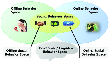
Figure 1: An illustration of composite behavior space.

We devote to proving that a high-quality (effective, quick-response, and robust) behavior model can be obtained by integrally using multi-dimensional behaviorial data, even though the quality of data is extremely insufficient in each dimension. For this challenging objective, a precondition is to solve users’ data insufficiency problem. The majority of users commonly have only several behavioral records that are too insufficient to build qualified behavior models. For this issue, we adopt a tensor decomposition-based method [37] by combining the similarity among users (in terms of interests to both tips and places) with social ties among them. Then, to fully utilize potential information in composite behaviors for user profiling, we propose a joint probabilistic generative model based on Bayesian networks, called Composite Behavioral Model (CBM). It offers a composition of the typical features in two different behavior spaces: check-in location in offline behavior space and UGC in online behavior space. Consider a composite behavior of a user, we assume that its generative mechanism is as follows: When a user plans to visit a venue and simultaneously post tips online, he/she subconsciously select a specific behavioral pattern according to his/her behavior distribution. Then, he/she comes up with a topic and a targeted venue based on the present pattern’s topic and venue distributions, respectively. Finally, his/her comment words are generated following the corresponding topic-word distribution. To estimate the parameters of the mentioned distributions, we adopt the collapsed Gibbs sampling [36].

Based on the joint model CBM, for each composite behavior, denoted by a triple-tuple $(u,v,\mathcal{D})$, we can calculate the chance of user $u$ visiting venue $v$ and posting a tip online with a set of words $\mathcal{D}$. Taking into account different levels of activity of different users, we devise a relative anomalous score $S_{r}$ to measure the occurrence rate of each composite behavior $(u,v,\mathcal{D})$. By these approaches, we finally realize a real-time (i.e., judging by only one composite behavior) detection for identity theft suspects.

We evaluate the proposed joint model by comparing with the typical models on two real-world OSN datasets: Foursquare [35] and Yelp [38]. We adopt the area under the receiver operating characteristic curve (AUC) as the detection efficacy. In the widely-used setting of theft simulation (simulating thefts via behavioral replacement) [39], the AUC value reaches $0.956$ in Foursquare and $0.947$ in Yelp, respectively. Particularly, the recall (True Positive Rate) reaches up to $65.3\%$ in Foursquare and $72.2\%$ in Yelp with the corresponding disturbance rate (False Positive Rate) below $1\%$. Note that these performances can be achieved by examining only one composite behavior per authentication, which guarantees the low response latency of our detection method. As an insightful result, we learn that the complementary effect does exist among different dimensions of low-quality records for modeling users’ behaviors. To the best of our knowledge, this is the first work jointly leveraging online and offline behaviors to detect identity theft in OSNs.

The rest of this paper is organized as follows. We give an overview of our solution in Section 2. Then, we present our method in Section 3, and make the validation in Section 4. We provide a literature review in Section 5. Finally, we draw conclusions in Section 6.

2 Overview of Our Solution

Online identity theft occurs when a thief steals a user’s personal data and impersonates the user’s account. Generally, a thief usually first gathers information about a targeted user to steal his/her identity and then use the stolen identity to interact with other people to get further benefits [9]. Criminals in different online services usually have different motivations. In this work, we focus on online social networks (OSNs). In some OSNs, one may know their online friends’ real-life identities. Thieves usually utilize the strong trust between friends to obtain benefit [40]. Their behavioral records usually contain specific sensitive terms. In other scenarios, friends may not be familiar with each other and lack direct interactions in the real world, which makes thieves can not obtain direct benefit from cheating users’ friends. So they turn to spread malicious messages in these OSNs. Among these malicious messages, some have explicit features such as URLs and contact numbers, others only contain deceptive comments on a place, a star or an event. The latter messages look like normal ones, which makes them harder to detect. Thus, we apply a widely-used setting of theft simulation, i.e., simulating thefts via behavioral replacement, to represent this kind of thieves.

An OSN user’s behavior is usually composite of online and offline behaviors occurring in different behavioral spaces, as illustrated in Fig. 1. Based on this fact, we aim to propose a joint model to embrace them into a unified model to deeply extract information.

Before introducing our joint model, named Composite Behavioral Model (CBM), we provide some conceptions as preparations. The relevant notations are listed in Table I.

TABLE I: Notations of Parameters

Variable	Description
$w$	the word in UGC
$v$	the venue or place
$\pi_{u}$	the community memberships of user $u$, expressed by a multinomial distribution over communities
$\theta_{c}$	the interests of community $c$, expressed by a multinomial distribution over topics
$\vartheta_{c}$	a multinomial distribution over spatial items specific to community $c$
$\phi_{z}$	a multinomial distribution over words specific to topic $z$
$\alpha,\beta,\gamma,\eta$	Dirichlet priors to multinomial distributions $\theta_{c}$, $\phi_{z}$, $\pi_{u}$ and $\vartheta_{c}$, respectively

Definition  1 (Composite Behavior).

A composite behavior, denoted by a four-tuple $(u,v,\mathcal{D},t)$, indicates that at time $t$, user $u$ visits venue $v$ and simultaneously posts online a tip consisting of a set of words $\mathcal{D}$.

We remark that for a composite behavior, the occurring time $t$ is a significant factor. Two types of time attributes play important roles in digging potential information for improving the identification. The first is the sequential correlation of behaviors. However, in real-life OSNs, the time intervals between adjacent recorded behaviors are mostly unknown or overlong, which leads that the temporal correlations cannot be captured effectively. The second is the temporal property of behaviors, e.g., periodicity and preference variance over time. However, in some real-life OSN datasets, the occurring time is recorded with a low resolution, e.g., by day, which shields the possible dependency of a user’s behavior on the occurring time. Thus, it is difficult to obtain reliable time-related features of users’ behaviors. Since we aim to propose a practical method based on uncustomized datasets of user behaviors, we only concentrate on the dependency between a user’s check-in location and tip-posting content of each behavior, taking no account of the impact of specific occurring time in this work. Thus, the representation of a composite behavior can be simplified into a triple-tuple $(u,v,\mathcal{D})$ without confusion in this paper.

Our model depends on the following assumptions: (1) Each user behaves in multiple patterns with different possibilities; (2) Some users have similar behavioral patterns, e.g., similar interests in topics and places.

To describe the features of users’ behaviors, we first introduce the topic of tips.

Definition  2 (Topic, [41]).

Given a set of words $\mathcal{W}$, a topic $z$ is represented by a multinomial distribution over words, denoted by $\mathbf{\phi}_{z}$, whose every component $\phi_{z,w}$ denotes the possibility of word $w$ occurring in topic $z$.

Next, we formulate a specific behavioral pattern of users by a conception called community.

Definition  3 (Community).

A community is a set of users with a similar behavioral pattern. Let $\mathcal{C}$ denote the set of all communities. A community $c\in\mathcal{C}$ has two critical parameters: (1) A topic distribution $\mathbf{\theta}_{c}$ whose component, say $\theta_{c,z}$, indicates the probability that users in community $c$ send a message with topic $z$. (2) A spatial distribution $\mathbf{\vartheta}_{c}$ whose component, say $\vartheta_{c,v}$, represents the chance that users in community $c$ visit venue $v$.

More specifically, we assume that a community is formed by the following procedure: Each user $u$ is included in communities according to a multinomial distribution, denoted by $\mathbf{\pi}_{u}$. That is, each component of $\mathbf{\pi}_{u}$, say $\pi_{u,c}$, denotes $u$’s affiliation degree to community $c$. Similarly, we allocate each community $c$ with a topic distribution $\mathbf{\theta}_{c}$ to represent its online topic preference and a spatial distribution $\mathbf{\vartheta}_{c}$ to represent its offline mobility pattern.

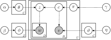
Figure 2: Graphical representation of joint model. The parameters are explained in Table I.

The graphical representation of our joint model CBM is demonstrated in Fig. 2.

3 Method

3.1 Composite Behavioral Model

Generally, users take actions according to their regular behavioral patterns which are represented by the corresponding communities (Definition 3). We present the behavioral generative process in Algorithm 1: When a user $u$ is going to visit a venue and post online tips there, he/she subconsciously select a specific behavioral pattern, denoted by community $c$, according to his/her community distribution $\mathbf{\pi}_{u}$ (Line $11$). Then, he/she comes up with a topic $z$ and a targeted venue $v$ based on the present community’s topic and venue distributions ($\mathbf{\theta}_{c}$ and $\mathbf{\vartheta}_{c}$, respectively) (Line $12-13$). Finally, the words of his/her tips in $\mathcal{D}$ are generated following the topic-word distribution $\mathbf{\phi}_{z}$ (Line $15$).

Algorithm 1 Joint Probabilistic Generative Process

1:  for each community $c\in\mathcal{C}$ do

2:     Sample the distribution over topics $\mathbf{\theta}_{c}\thicksim Dirichlet(\cdot|\alpha)$

3:     Sample the distribution over venues $\mathbf{\vartheta}_{c}\thicksim Dirichlet(\cdot|\eta)$

4:  end for

5:  for each topic $z\in\mathcal{Z}$ do

6:     Sample the distribution over words $\mathbf{\phi}_{z}\thicksim Dirichlet(\cdot|\beta)$

7:  end for

8:  for each user $u\in\mathcal{U}$ do

9:     Sample the distribution over communities $\mathbf{\pi}_{u}\thicksim Dirichlet(\cdot|\gamma)$

10:     for each composite behavior $(u,v,\mathcal{D})\in\mathcal{B}_{u}$ do

11:        Sample a community indicator $c\thicksim Multi(\mathbf{\pi}_{u})$

12:        Sample a topic indicator $z\thicksim Multi(\mathbf{\theta}_{c})$

13:        Sample a venue $v\thicksim Multi(\mathbf{\vartheta}_{c})$

14:        for each word $w\in\mathcal{D}$ do

15:           Sample a word $w\thicksim Multi(\mathbf{\phi}_{z})$

16:        end for

17:     end for

18:  end for

Exact inference of our joint model CBM is difficult due to the intractable normalizing constant of the posterior distribution, [36]. We adopt collapsed Gibbs sampling for approximately estimating distributions (i.e., $\mathbf{\theta}$, $\mathbf{\vartheta}$, $\mathbf{\phi}$ and $\mathbf{\pi}$). As for the hyperparameters, we take a fixed value, i.e., $\alpha=50/Z$, $\gamma=50/C$ and $\beta=\eta=0.01$, following the study in [42], where $Z$ and $C$ are the numbers of topics and communities, respectively.

In each iteration, for each composite behavior $(u,v,\mathcal{D})$, we first sample community $c$ according to Eq. (1):

$$P(c|\mathbf{c^{\neg}},\mathbf{z},\mathbf{v},u)\propto(n_{u,c}^{\neg}+\gamma)\frac{n_{c,z}^{\neg}+\alpha}{\sum_{z^{\prime}}(n_{c,z^{\prime}}^{\neg}+\alpha)}\frac{n_{c,v}^{\neg}+\eta}{\sum_{v^{\prime}}(n_{c,v^{\prime}}^{\neg}+\eta)},$$ (1)

where $\mathbf{c^{\neg}}$ denotes the community allocation for all composite behaviors except the current one; $\mathbf{z}$ denotes the topic allocation for all composite behaviors; $n_{u,c}$ denotes the number of times that community $c$ is generated by user $u$; $n_{c,z}$ denotes the number of times that topic $z$ is generated by community $c$; $n_{c,v}$ denotes the number of times that venue $v$ is visited by users in community $c$; a superscript $\neg$ denotes something except the current one.

Then, given a community $c$, we sample topic $z$ according to the following Eq. (2):

$$P(z|\mathbf{z^{\neg}},\mathbf{c},\mathcal{D})\propto(n_{c,z}^{\neg}+\alpha)\prod_{w\in\mathcal{D}}\frac{n_{z,w}^{\neg}+\beta}{\sum_{w^{\prime}}(n_{z,w^{\prime}}^{\neg}+\beta)},$$ (2)

where $n_{z,w}$ denotes the number of times that word $w$ is generated by topic $z$.

The inference algorithm is presented in Algorithm 2. We first randomly initialize the topic and community assignments for each composite behavior (Line $2-4$). Then, we update the community and topic assignments for each composite behavior based on Eqs. (1) and (2) in each iteration (Line $6-9$). Finally, we estimate the parameters, test the coming cases and update the training set every $I_{s}$ iterations since $I_{b}$th iteration (Line $10-13$) to address concept drift.

Algorithm 2 Inference Algorithm of the Joint Model CBM

0:  user composite behavior collection $\mathcal{B}$, number of iteration $I$, start saving step $I_{b}$, saving lag $I_{s}$, start training sequence number $N_{b}$, end training sequence number $N_{e}$, hyperparameters $\alpha$, $\beta$, $\gamma$ and $\eta$

0:  estimated parameters $\hat{\mathbf{\theta}}$, $\hat{\mathbf{\vartheta}}$, $\hat{\mathbf{\phi}}$, $\hat{\mathbf{\pi}}$

1:  Create temporary variables $\mathbf{\theta^{sum}}$, $\mathbf{\vartheta^{sum}}$, $\mathbf{\phi^{sum}}$ and $\mathbf{\pi^{sum}}$, initialize them with zero, set testing sequence number $N_{t}=0$ and let $\mathcal{B}(N_{t})$ denotes the corresponding training collection for testing behaviors which sequence number values $N_{t}$

2:  for each composite behavior $(u,v,\mathcal{D})\in\mathcal{B}(N_{t})$ do

3:     Sample community and topic randomly

4:  end for

5:  for $iteration=1$ to $I$ do

6:     for each behavior $(u,v,\mathcal{D})\in\mathcal{B}(N_{t})$ do

7:        Sample community $c$ according to Eq. (1)

8:        Sample topic $z$ according to Eq. (2)

9:     end for

10:     if $(iteration>I_{b})$ and $(iteration~{}mod~{}I_{s}==0)$ then

11:        return  model parameters as follows: $\theta_{c,z}=\frac{n_{c,z}+\alpha}{\sum_{z^{\prime}}(n_{c,z^{\prime}}+\alpha)}$; $~{}~{}\vartheta_{c,v}=\frac{n_{c,v}+\eta}{\sum_{v^{\prime}}(n_{c,v^{\prime}}+\eta)}$ $\pi_{u,c}=\frac{n_{u,c}+\gamma}{\sum_{c^{\prime}}(n_{u,c^{\prime}}+\gamma)}$; $~{}~{}\phi_{z,w}=\frac{n_{z,w}+\beta}{\sum_{w^{\prime}}(n_{z,w^{\prime}}+\beta)}$

12:        Evaluate corresponding test cases and update $N_{t}++$; $N_{b}++$; $N_{e}++$

13:     end if

14:  end for

To overcome the problem of data insufficiency, we adopt the tensor decomposition [37] to discover their potential behaviors. In our experiment, we use the Twitter-LDA [43] to obtain each UGC’s topic and construct a tensor $\mathbf{A}\in\mathbb{R}^{N\times M\times L}$, with three dimensions standing for users, venues and topics. Then, $\mathbf{A}(u,v,z)$ denotes the frequency that user $u$ posting a message on topic $z$ in venue $v$. We can decompose $\mathbf{A}$ into the multiplication of a core tensor $\mathbf{S}\in\mathbb{R}^{d_{U}\times d_{V}\times d_{Z}}$ and three matrices, $\mathbf{U}\in\mathbb{R}^{N\times d_{U}}$, $\mathbf{V}\in\mathbb{R}^{M\times d_{V}}$, and $\mathbf{Z}\in\mathbb{R}^{L\times d_{Z}}$, if using a tucker decomposition model, where $d_{U}$, $d_{V}$ and $d_{Z}$ denote the number of latent factors; $N$, $M$ and $L$ denote the number of users, venues and topics. An objective function to control the errors is defined as:

$$\begin{split}&\mathcal{L}(\mathbf{S},\mathbf{U},\mathbf{V},\mathbf{Z})=\frac{1}{2}{\|\mathbf{A}-\mathbf{S}\times_{U}\mathbf{U}\times_{V}\mathbf{V}\times_{Z}\mathbf{Z}\|}^{2}\\ &+\frac{\lambda}{2}\left({\|\mathbf{S}\|}^{2}+{\|\mathbf{U}\|}^{2}+{\|\mathbf{V}\|}^{2}+{\|\mathbf{Z}\|}^{2}+\sum\nolimits_{(i,j)\in\mathcal{F}}u_{i}^{T}u_{j}\right),\end{split}$$

where $\mathcal{F}$ is a set of friend pairs $(i,j)$. $\mathbf{A}^{*}=\mathbf{S}\times_{U}\mathbf{U}\times_{V}\mathbf{V}\times_{Z}\mathbf{Z}$ is the potential frequency tensor, and $\mathbf{A}^{*}(u,v,z)$ denotes the frequency that user $u$ may post a message on topic $z$ in venue $v$. A higher $\mathbf{A}^{*}(u,v,z)$ indicates that user $u$ has a higher chance to do this kind of behavior in the future. We limit the competition space to the behavior space of $u$’s friends, i.e.,

$$\left\{(u,v,z)|\mathbf{A}(u^{{}^{\prime}},v,z)>0,(u,u^{{}^{\prime}})\in\mathcal{F}\right\},$$

and select the top $20$ behaviors as his/her latent behavior to improve data quality.

3.2 Identity Theft Detection Scheme

By the parameters $\hat{\mathbf{\Psi}}=\{\hat{\mathbf{\theta}},\hat{\mathbf{\vartheta}},\hat{\mathbf{\phi}},\hat{\mathbf{\pi}}\}$ learnt from the inference algorithm (Algorithm 2), we can estimate the logarithmic anomalous score $(S_{l})$ of a composite behavior $(u,v,\mathcal{D})$ by Eq. (3):

$$\begin{split}S_{l}(u,v,\mathcal{D})&=-\lg P(v,\mathcal{D}|u)\\ &=-\lg\left(\sum_{c}{\hat{\pi}_{u,c}\hat{\vartheta}_{c,v}\sum_{z}{\hat{\theta}_{c,z}(\prod_{w\in\mathcal{D}}\hat{\phi}_{z,w})^{\frac{1}{|\mathcal{D}|}}}}\right).\end{split}$$ (3)

However, we may mistake some normal behaviors occurring with low probability, e.g., the normal behaviors of users whose behavioral diversity and entropy are both high, for suspicious behaviors. Thus, we propose a relative anomalous score $(S_{r})$ to indicate the trust level of each behavior by Eq. (4):

$$S_{r}(u,v,\mathcal{D})=1-P(u|v,\mathcal{D})=1-\frac{P(v,\mathcal{D}|u)P(u)}{\sum_{u^{\prime}}P(v,\mathcal{D}|u^{\prime})P(u^{\prime})}.$$ (4)

We randomly select $40$ users to estimate the relative anomalous score for each composite behavior. Our experimental results in Section 4 show that the approach based on $S_{r}$ outperforms the approach based on $S_{l}$.

4 Evaluation

In this section, we present the experimental results to evaluate the proposed joint model CBM, and validate the efficacy of the joint model for identity theft detection on real-world OSN datasets.

4.1 Datasets

Our experiments are conducted on two real-life large OSN datasets: Foursquare [35] and Yelp [38].

TABLE II: Statistics of Foursquare and Yelp Datasets

	Foursquare	Yelp
# of users	31,493	80,592
# of venue	143,923	42,051
# of check-ins	267,319	491,393

They are two well-known online social networking service providers. In both datasets, there is no URLs or other sensitive terms. Both datasets contain users’ social ties and behavioral records. Each social tie contains user-ID and friend-ID. Each behavior record contains user-ID, venue-ID, timestamp and UGC. Their basic statistics are shown in Table II.

We count each user’s records, and present the results in Fig. 3. It shows that most users have less than $5$ records in both datasets. The quality of these dataset is too poor to model individual-level behavioral patterns for the majority of users, which confronts our method with a big challenge.

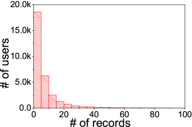
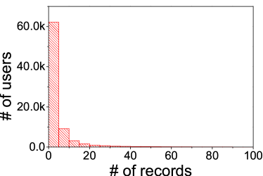
(a) Foursquare.	(b) Yelp.

Figure 3: The distribution of user record counts.

4.2 Experiment Settings

4.2.1 Suspicious Behavior Simulation

Many works [8, 44, 29] aimed at discovery theft’s behavioral pattern. Bursztein et al. [40] pointed out that identity thieves usually behave in two possible suspicious patterns, i.e., (1) behaving unlike the majority of users; (2) behaving only unlike the victim. Many existing outlier detecting techniques, e.g., i-Forest [45], LOF [46] and GSDPMM [47] can deal with the former cases. Besides, we notice that the former can be regarded as a special case of the latter. It is straightforward that an effective detection method for the latter can apply effectively to the former cases. If the experiments validate that our model performs well even for detecting such crafty thieves, a strong argument can be obtained to prove the capability of our model. This is the reason why we focus on the latter cases where thieves tend to hind them among the people.

In the experiments, we use two real-life datasets, and assume that all records are normal behaviors. We simulate suspicious behaviors by exchanging some users’ behavioral records and setting them as positive instances [40]. This theft simulation process imitates one kind of the most crafty thieves who behave just like normal users. More specifically, we first rank behavior records according to their timestamps. Then, we select the top $80\%$ behavior records for training and the rest for testing. To simulate suspicious behaviors, we randomly exchange $5\%$ of all behavior records in the test set as anomalous behaviors. Totally, we have $56,236$ test behaviors in Foursquare and $71,667$ in Yelp, and make up $2,884$ anomalous behaviors in Foursquare and $3,583$ in Yelp, respectively.

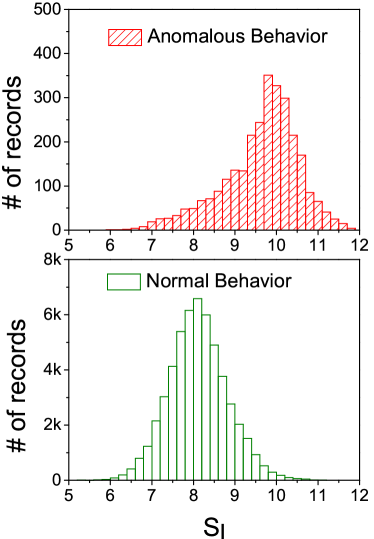
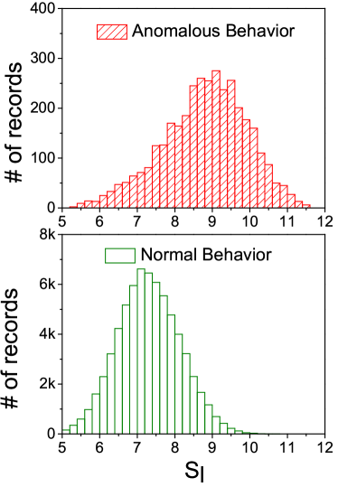
(a) Foursquare	(b) Yelp

Figure 4: The histogram of logarithmic anomalous score $S_{l}$ (defined in Eq. (3)) for each behavior.

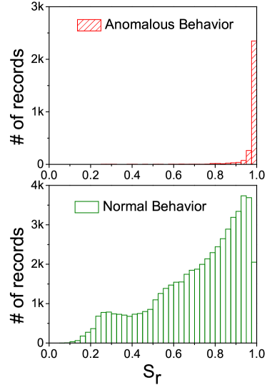
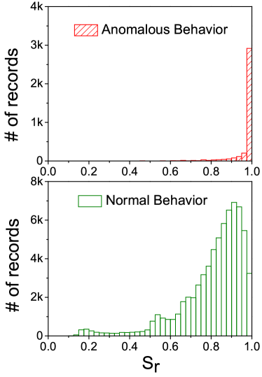
(a) Foursquare	(b) Yelp

Figure 5: The histogram of relative anomalous score $S_{r}$ (defined in Eq. (4)) for each behavior.

4.2.2 Metrics

For the convenience of description, we first give a confusion matrix in Table III.

TABLE III: Confusion Matrix for Binary Classification.

Predicted Condition	True Condition
	Positive	Negative
Positive	True Positive (TP)	False Positive (FP)
Negative	False Negative (FN)	True Negative (TN)

In the experiments, we set anomalous behaviors as positive instances, and focus on the following four metrics, since the identity theft detection is essentially an imbalanced binary classification problem [48].

True Positive Rate (TPR): TPR is computed by $\frac{TP}{TP+FN}$, and indicates the proportion of true positive instances in all positive instances (i.e., the proportion of anomalous behaviors that are detected in all anomalous behaviors). It is also known as recall. Specifically, we named it detection rate.

False Positive Rate (FPR): FPR is computed by $\frac{FP}{FP+TN}$, and indicates the proportion of false positive instances in all negative instances (i.e., the proportion of normal behaviors that are mistaken for anomalous behaviors in all normal behaviors). Specifically, we named it disturbance rate.

Precision: The precision is computed by $\frac{TP}{TP+FP}$, and indicates the proportion of true positive instance in all predicted positive instance (i.e., the proportion of anomalous behaviors that are detected in all suspected cases).

AUC: Given a rank of all test behaviors, the AUC value can be interpreted as the probability that a classifier/predictor will rank a randomly chosen positive instance higher than a randomly chosen negative one.

4.2.3 Threshold Selection

It is an important issue in classification tasks. Recall that for the hyper-parameters $\alpha$, $\beta$, $\gamma$ and $\eta$, we adopt a fixed value, i.e., $\alpha=50/Z$, $\gamma=50/C$ and $\beta=\eta=0.01$, following the study [36]. Specifically, we take the case that $C=30$ and $Z=20$ as an example to present the threshold selection strategy. The parameter sensitivity analysis will be conducted in the following Section 4.2.4. We compare the distribution of logarithmic anomalous score $S_{l}$ (or relative anomalous score $S_{r}$) for normal behaviors with that for anomalous behaviors. Figs. 4 and 5 present the differences between normal and anomalous behaviors in terms of the distributions of $S_{l}$ and $S_{r}$, respectively. They show that the differences are both significant, and the difference in terms of $S_{r}$ is much more obvious.

To obtain a reasonable threshold, we focus on the performance where the threshold changes from $0.975$ to $1$, since this range contains $81.5\%$ ($81.4\%$) of all anomalous behaviors and $3.9\%$ ($4.8\%$) of all normal behaviors in Foursquare (Yelp). The detailed trade-offs are demonstrated in Figs. 6 and 7 from different aspects. To optimize the trade-offs of detection performance, we define the detection Cost in Eq. (5):

$$Cost=\frac{\#\mbox{ of newly mistaken normal behaviors}}{\#\mbox{ of newly identified anomalous behaviors}}.$$ (5)

We present the threshold-cost curve in Fig. 8. It shows that a smaller threshold usually corresponds to a larger cost.

We select the minimum threshold satisfying that the corresponding cost is less than $1$. Thus, we choose $0.989$ and $0.992$ as the thresholds for Foursquare and Yelp, respectively. Under them, our joint model CBM reaches $62.32\%$ ($68.75\%$) in TPR and $0.85\%$ ($0.71\%$) in FPR on Foursquare (Yelp). Please refer to Table IV for details.

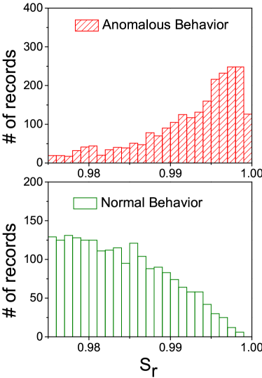
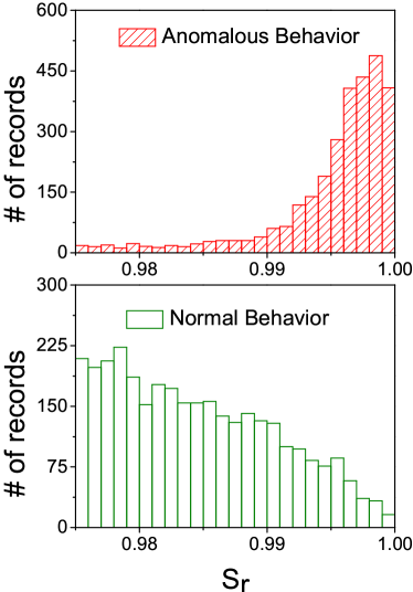
(a) Foursquare	(b) Yelp

Figure 6: A partial of the distribution of relative anomalous score $S_{r}$ (defined in Eq. (4)) for each behavior.

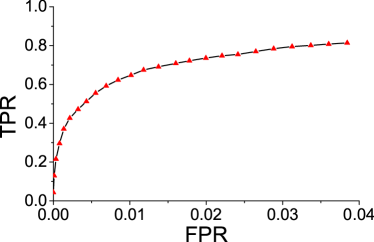
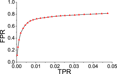
(a) Foursquare	(b) Yelp

Figure 7: A partial of ROC (receiver operating characteristic) curve of identity theft detection.

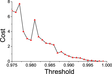
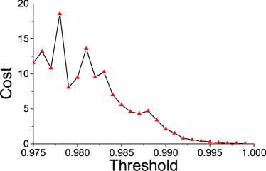
(a) Foursquare	(b) Yelp

Figure 8: Detection costs with different thresholds.

TABLE IV: A Summary of Different Metrics [49] with the Threshold $0.989$ for Foursquare and $0.992$ for Yelp.

	Foursquare	Yelp
AUC	0.956	0.947
Precision	79.91%	83.55%
Recall (TPR)	62.32%	68.75%
FPR	0.85%	0.71%
TNR	99.15%	99.29%
FNR	37.68%	31.25%
Accuracy	97.26%	97.76%
F1	0.700	0.754

4.2.4 Parameter Sensitivity Analysis

Parameter tuning is another important part of our work. The performance of our model is indeed sensitive to the number of communities ($C$) and topics ($Z$). Therefore, we study the impact of varying parameters in our model. We select the relative anomalous score $S_{r}$ as the test variable, and evaluate the performance of our model by changing the values of $C$ and $Z$. The experimental results are summarized in Tables V.

TABLE V: AUC on Foursquare (Yelp) Dataset

	C=10	C=20	C=30
Z=10	0.876 (0.910)	0.945 (0.936)	0.953 (0.945)
Z=20	0.917 (0.915)	0.946 (0.938)	0.956 (0.947)
Z=30	0.922 (0.917)	0.947 (0.938)	0.957 (0.947)

From the results on both datasets, the detection efficacy goes stable when the number of topics reaches $20$ and the number of communities has a larger impact on the efficacy. Thus, we set $C=30$ and $Z=20$ in our joint model, and present the receiver operating characteristic (ROC) and Precision-Recall curves in Figs. 9 and 10, respectively. Specifically, we present detection rate (TPR) in Table VI, where disturbance rate (FPR) reaches 1% and 0.1%, respectively.

TABLE VI: Detection Rates with Different Disturbance Rates.

	Foursquare	Yelp
Disturbance Rate=0.1%	30.8%	31.7%
Disturbance Rate=1.0%	65.3%	72.2%

(a) Foursquare	(b) Yelp

Figure 9: The ROC curves of identity theft detection via the joint model CBM.

(a) Foursquare	(b) Yelp

Figure 10: The Precision-Recall curves of identity theft detection via the joint model CBM.

4.3 Performance Comparison

4.3.1 Representative Models

We compare our joint model CBM to some representative models in OSNs. In Table VII, we list the features of these models.

TABLE VII: Behaviors Adopted in Different Models

	Online Behavior (UGC)	Offline Behavior (Check-in)
CF-KDE	NO	YES
LDA	YES	NO
FUSED	YES	YES
JOINT	YES	YES

CF-KDE. Before presenting the CF-KDE model, we introduce the Mixture Kernel Density Estimate (MKDE) [39] to give a brief prior knowledge on Kernel Density Estimate (KDE). MKDE is an individual-level spatial distribution model based on KDE. It is a typical spatial model describing user’s offline behavioral pattern. In this model, it mainly utilizes a bivariate density function in the following equations to capture the spatial distribution for each user:

$$f_{KDE}\left(e|E,h\right)=\frac{1}{n}\sum\nolimits_{j=1}^{n}K_{h}\left(e-e^{j}\right),$$ (6)

$$K_{h}\left(x\right)=\frac{1}{2\pi h}\exp\left(-\frac{1}{2}x^{T}H^{-1}x\right),\mathbf{H}=\begin{pmatrix}h&0\\ 0&h\end{pmatrix},$$ (7)

$$f_{MKDE}\left(e|E,h\right)=\alpha f_{KD}\left(e|E_{1}\right)+\left(1-\alpha\right)f_{KD}\left(e|E_{2}\right).$$ (8)

In Eq. (6), $E=\{e^{1},...,e^{n}\}$ is a set of historical behavioral records for a user and $e^{j}=<x,y>$ is a two-dimensional spatial location (i.e., offline behavior). Eq. (7) is a kernel function and $\mathbf{H}$ is the bandwidth matrix. MKDE adopts Eq. (8), where $E_{1}$ is a set of an individual’s historical behavioral records (individual component), $E_{2}$ is a set of his/her friends’ historical behavioral records (social component), and $\alpha$ is the weight variable for individual component. To detect identity thieves, we compute a surprise index $S_{e}$ in Eq. (9) for each behavior $e$, defined as the negative log-probability of individual $u$’s conducting behavior $e$:

$$S_{e}=-\log f_{MKDE}\left(e|E_{u},h_{u}\right).$$ (9)

Furthermore, we can select the top-$N$ behaviors with the highest $S_{e}$ as suspicious behaviors.

In MKDE model, it assumes that users tend to do like their friends in the same chance. It has not quantified the potential influence of different friends. Thus, we introduce a collaborative filtering method to improve the performance. Based on the historical behavioral records, it establishes a user-venue matrix $\mathbf{R}_{|\mathbf{U}|\times|\mathbf{V}|}$, where $U$ and $V$ are the number of users and venues, respectively; $\mathbf{R}_{ij}=1$ if user $i$ has visited venue $j$ in the training set, otherwise $\mathbf{R}_{ij}=0$. We adopt a matrix factorization method with an objective function in Eq. (10) to obtain feature vectors for each user and venue:

$$L=\min_{\mathbf{U},\mathbf{V}}\frac{1}{2}\sum_{i=1}^{U}\sum_{j=1}^{V}(\mathbf{R}_{ij}-u_{i}^{T}v_{j})^{2}+\frac{\lambda_{1}}{2}\sum_{i=1}^{U}u_{i}^{T}u_{i}+\frac{\lambda_{2}}{2}\sum_{j=1}^{V}v_{j}^{T}v_{j}.$$ (10)

Specifically, we let

$u_{i}=(u_{i}^{(1)},u_{i}^{(2)},...,u_{i}^{(k)})^{T}$ and $v_{j}=(v_{j}^{(1)},v_{j}^{(2)},...,v_{j}^{(k)})^{T}$.

We adopt a stochastic gradient descent algorithm in Eqs. (11) and (12) in the optimization process:

$$u_{i}^{(k)}\leftarrow u_{i}^{(k)}-\alpha(\sum\nolimits_{j=1}^{V}(\mathbf{R}_{ij}-u_{i}^{T}v_{j})v_{j}^{(k)}+\lambda_{1}u_{i}^{(k)}),$$ (11)

$$v_{j}^{(k)}\leftarrow v_{j}^{(k)}-\alpha(\sum\nolimits_{i=1}^{U}(\mathbf{R}_{ij}-u_{i}^{T}v_{j})u_{i}^{(k)}+\lambda_{2}v_{j}^{(k)}).$$ (12)

Consequently, we can figure out $\hat{\mathbf{R}}=\mathbf{U}^{T}\mathbf{V}$, and use $\hat{r}_{ij}=u_{i}^{T}v_{j}$ as the weight variable for the KDE model. To detect anomalous behaviors, we use Eq. (13) to measure the surprising index for each behavior $e$:

$$S_{e}=-\log\frac{\sum_{j=1}^{n}\hat{r}_{uj}K_{h}\left(e-e^{j}\right)}{\sum_{j=1}^{n}\hat{r}_{uj}}.$$ (13)

Furthermore, we can select the top-$N$ behaviors with the highest $S_{e}$ as suspicious behaviors.

LDA. Latent Dirichlet Allocation (LDA) [41] is a classic topic model. User’s online behavior pattern can be denoted as the mixing proportions for topics. We aggregate the UGC of each user and his/her friends in the training set as a document, then use LDA to obtain each user’s historical topic distribution $\theta_{his}$. To get their present behavioral topic distribution $\theta_{new}$ in the test set. For each behavior, we count the number of words assigned to the $k$th topic, and denoted it as $n(k)$. The $k$th component of the topic proportion vector can be computed in Eq. (14):

$$\theta_{new}^{(k)}=\frac{n\left(k\right)+\alpha}{\sum_{i=1}^{K}(n\left(i\right)+\alpha)},$$ (14)

where $K$ is the number of topics, and $\alpha$ is a hyperparameter. Specifically, we set $\alpha=50/K$.

To detect anomalous behaviors, we measure the distance between a user’s historical and present topic distribution by using the Jensen-Shannon (JS) divergence in Eqs. (15) and (16):

$$D_{KL}\left(\theta_{his},\theta_{new}\right)=\sum\nolimits_{i=1}^{K}\theta_{his}^{(i)}\cdot\ln\left({\theta_{his}^{(i)}}/{\theta_{new}^{(i)}}\right),$$ (15)

$$D_{JS}\left(\theta_{his},\theta_{new}\right)=\frac{1}{2}\left[D_{KL}\left(\theta_{his},M\right)+D_{KL}\left(\theta_{new},M\right)\right].$$ (16)

where $M=\frac{\theta_{his}+\theta_{new}}{2}$. We can select the top-$N$ behaviors with the highest $D_{JS}(\theta_{his},\theta_{new})$ as suspicious behaviors.

Fused Model. Egele et al. [8] propose COMPA which directly combining use users’ explicit behavior features, e.g., language, links, message source, et al. In our case, we setup a fused model, which deep combine users’ implicit behavior features discovered by CF-KDE and LDA to detect identity theft. We try different thresholds for the CF-KDE model and LDA model (i.e., different classifiers). For each pair (i.e., a CF-KDE model and an LDA model), we treat any behavior that fails to pass either identification model as suspicious behavior, and compute true positive rate and false positive rate to draw the ROC curve and estimate the AUC value.

4.3.2 Performance Comparison

We compare the performance of our method with the typical ones in terms of detection efficacy (AUC) and response latency. The latter denotes the number of behaviors in the test set needed to cumulate for detecting a specific identity theft case.

Detection Efficacy Analysis. In Fig. 11, we present the results of all comparison methods.

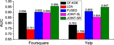
Figure 11: Identity theft detection efficacy.

Our joint model outperforms all other methods on the two datasets. The AUC value reaches $0.956$ and $0.947$ in Foursquare and Yelp datasets, respectively.

There are three reasons for its outstanding performance. Firstly, it embraces different types of behaviors and exploits them in a unified model. Secondly, it takes advantage of the community members’ and friends’ group-level behavior patterns to overcome the data insufficiency and concept drift [40] in individual-level behavioral patterns. Finally, it utilizes correlations among different behavioral spaces.

From the results, we have several other interesting observations: (1) LDA model performs poor in both datasets which may indicate its performance is strongly sensitive to the data quality. (2) CF-KDE and LDA model performs not well in Yelp dataset comparing to Foursquare dataset, but the fused model observes a surprising reversion. (3) The joint model based on relative anomalous score $S_{r}$ outperforms the model based on logarithmic anomalous score $S_{l}$. (4) The joint model (i.e., JOINT-SR, the joint model in the following sections all refer to the joint model based on $S_{r}$) is indeed superior to the fused model.

Response Latency Analysis. For each model, we also evaluate the relationship between the efficacy and response latency (i.e., a response latency $k$ means that the identity theft is detected based on $k$ recent continuous behaviors). Figs. 12 and 13 demonstrate the AUC values and TPRs via different response latency in each model on both datasets.

The experimental results indicate that our joint model CBM is superior to all other methods. The AUC values of our joint model can reach $0.998$ in both Foursquare and Yelp with $5$ test behavioral records. The detection rates (TPR) of our joint model can reach $93.8\%$ in Foursquare and $97.0\%$ in Yelp with $5$ test behavioral records and disturbance rate (FPR) values $1.0\%$.

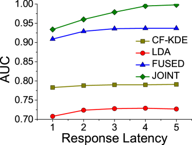
(a) Foursquare	(b) Yelp

Figure 12: Identity theft detection efficacy via different response latency (i.e., the number of behaviors in the test set we cumulated).

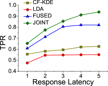
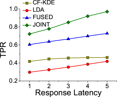
(a) Foursquare	(b) Yelp

Figure 13: The detection rates (TPR) via different response latency with disturbance rate=0.01 (FPR=0.01).

4.3.3 Robustness Analysis

Generally, there are two kinds of mutations in individual-level (IL) suspicious behavioral patterns:

Completely Behavioral Mutation. Some thieves tore off their masks once intruding into victim’s account. They usually perform totally different interest in venues and topics.

Partially Behavioral Mutation. Some extremely cunning thieves maintain part of victim’s behavioral pattern to get further benefits from the victim’s friends. They may show partial behavior mutation which makes it harder to detect these anomalous behaviors.

In the previous experiments, we evaluate the performance of our model in a scenario where thieves act like normal users by exchanging normal user’s behavioral records (exchanging both venue and UGC). Furthermore, we consider the harder scenarios where thieves know part of victim’s habits and accordingly imitate victims. We apply our model to these scenarios, and demonstrate experimental results in Fig. 14. The results validate that our method is robust for coping with various suspicious behaviors.

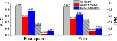
Figure 14: The efficacy (AUC) and detection rate (TPR) of identity theft detection via the joint model CBM in different scenarios with disturbance rate=0.01 (FPR=0.01). Painted ones denote AUC and shaded ones denote TPR.

4.4 Explanations on Advantages of Joint Model

4.4.1 Intuitive Explanations

Generally, there are two paradigms to integrate behavioral data: the fused and joint manners [8] . Fused models [8] are a relatively simple and straightforward kind of composite behavior models. They first capture features in each behavior space respectively, and then make a comprehensive metric based on these features in different dimensions. With the possible complementary effect among different behavior spaces, they can act as a feasible solution for integration. However, the identification efficacy can be further improved, since fused models neglect potential links among different spaces of behaviors. We take an example where a person posted a picture in an OSN when he/she visited a park. If this composite behavior is simply separated into two independent parts: he/she once posted a picture and he/she once visited a park, the difficulty in relocating him/her from a group of users is possibly increased, since there are more users satisfy these two simple conditions comparing to the original condition.

On the contrast, our joint model CBM sufficiently exploits the correlations between behaviors in different dimensions, then increases the certainty of users’ behavior patterns, which contributes to a better identification efficacy.

4.4.2 Theoretical Explanation

We provide an underlying information theoretical explanation for the gain of joint models. The well-known Chain Rule for Entropy [50],

$$H(X_{1},X_{2},...,X_{N})\leq\sum\nolimits_{i=1}^{N}H(X_{i}),$$

indicates that the entropy of $N$ simultaneous events, denoted by $X_{i}$, $i=1,2,\cdots,N$, is no more than the sum of the entropies of each individual event, and are equal if the events are independent.

The chain rule for entropy shows that the joint behavior has lower uncertainty comparing to the sum of the uncertainty in each component [51]. This can serve as a theoretical explanation of the advantages of our joint model.

5 Literature Review

Recently, researchers found that users’ behavior can identify their identities[3, 52, 28]. Typically, behavior-based user identification include two phases: user profiling and user identifying:

User profiling is a process to characterize a user with his/her history behavioral data. Some works focus on statistical characteristics to establish the user profile. Naini et al. [53] studied the task of identifying the users by matching the histograms of their data in the anonymous dataset with the histograms from the original dataset. Egele et al. [8] proposed a behavior-based method to identify compromises of high-profile accounts. Ruan et al. [30] conducted a study on online user behavior by collecting and analyzing user clickstreams of a well known OSN. Lesaege et al. [29] developed a topic model extending the Latent Dirichlet Allocation (LDA) to identify the active users. Viswanath et al. [44] presented a technique based on Principal Component Analysis (PCA) that accurately modeled the “like” behavior of normal users in Facebook and identified significant deviations from it as anomalous behaviors. Tsikerdekis and Zeadally [54] presented a detection method based on nonverbal behavior for identity deception, which can be applied to many types of social media. These methods above mainly concentrated on a specific dimension of the composite behavior without utilizing the correlations among multi-dimensional behavior data.

Vedran et al. [55] explored the complex interaction between social and geospatial behavior and demonstrated that social behavior can be predicted with high precision. Yin et al. [36] proposed a probabilistic generative model combining use spatiotemporal data and semantic information to predict user’s behavior. These studies implied that composite behavior features are possibly helpful for user identification.

User identifying is a process to match the same user in two datasets or distinguish anomalous users/behaviors. User identifying can be applied to a variety of tasks, such as detecting anomalous users or match users across different data sources. Mazzawi et al. [56] presented a novel approach for detecting malicious user activity in databases by checking user’s self-consistency and global-consistency. Lee and Kim [32] proposed a suspicious URL detection system for Twitter to detect users’ anomalous behaviors. Cao et al. [22] designed and implemented a malicious account detection system for detecting both fake and compromised real user accounts. Zhou et al. [57] proposed an FRUI algorithm to match users among multiple OSNs. These works mainly detected the population-level anomalous behaviors which indicated strongly difference from other behaviors. While, they did not consider that the individual-level coherence of users’ behavioral patterns can be utilized to detect online identity thieves.

6 Conclusion and Future Work

We investigate the feasibility in building a ladder from low-quality behavioral data to a high-quality behavioral model for user identification in online social networks (OSNs). By exploiting the complementary effect among OSN users’ multi-dimensional behaviors, we propose a joint probabilistic generative model by integrating online and offline behaviors. When the designed model is applied into identity theft detection in OSNs, its comprehensive performance, in terms of the detection efficacy, response latency and robustness, is validated by extensive evaluations implemented on real-life OSN datasets. This study gives new insights into whether and how modeling users’ composite behavioral patterns can improve online identity authentication.

Our behavior-based module mainly aims at detecting identity thieves after the the access control of account is broken. It is not exclusive to the traditional methods for preventing identity theft. On the contrary, it is easy to incorporate our module into traditional methods to solve identity theft problem better, since our method is non-intrusive and continuous. We would like to leave the study on the combinations of preventing and detecting methods from a systematic perspective as future work.

References

- [1] J. Onaolapo, E. Mariconti, and G. Stringhini, “What happens after you are pwnd: Understanding the use of leaked webmail credentials in the wild,” in Proc. IMC 2016, 2016, pp. 65–79.
- [2] A. Mohan, “A medical domain collaborative anomaly detection framework for identifying medical identity theft,” in Proc. CTS 2014, 2014, pp. 428–435.
- [3] Y.-A. De Montjoye, L. Radaelli, V. K. Singh et al., “Unique in the shopping mall: On the reidentifiability of credit card metadata,” Science, vol. 347, no. 6221, pp. 536–539, 2015.
- [4] P. Hyman, “Cybercrime: it’s serious, but exactly how serious?” Commun. ACM, vol. 56, no. 3, pp. 18–20, 2013.
- [5] J. Lynch, “Identity theft in cyberspace: Crime control methods and their effectiveness in combating phishing attacks,” Berkeley Technology Law Journal, pp. 259–300, 2005.
- [6] L. Bilge, T. Strufe, D. Balzarotti, and E. Kirda, “All your contacts are belong to us: automated identity theft attacks on social networks,” in Proc. WWW 2009, 2009, pp. 551–560.
- [7] G. Newman and M. M. McNally, “Identity theft literature review,” 2005.
- [8] M. Egele, G. Stringhini, C. Kruegel, and G. Vigna, “Towards detecting compromised accounts on social networks,” IEEE Trans. Dependable Sec. Comput., vol. 14, no. 4, pp. 447–460, 2017.
- [9] K. Thomas, F. Li, A. Zand, J. Barrett, J. Ranieri, L. Invernizzi, Y. Markov, O. Comanescu, V. Eranti, A. Moscicki, D. Margolis, V. Paxson, and E. Bursztein, “Data breaches, phishing, or malware?: Understanding the risks of stolen credentials,” in Proc. CCS 2017, 2017, pp. 1421–1434.
- [10] T. C. Pratt, K. Holtfreter, and M. D. Reisig, “Routine online activity and internet fraud targeting: Extending the generality of routine activity theory,” Journal of Research in Crime and Delinquency, vol. 47, no. 3, pp. 267–296, 2010.
- [11] K. Thomas, C. Grier, J. Ma, V. Paxson, and D. Song, “Design and evaluation of a real-time URL spam filtering service,” in Proc. IEEE S&P 2011, 2011, pp. 447–462.
- [12] A. M. Marshall and B. C. Tompsett, “Identity theft in an online world,” Computer Law & Security Review, vol. 21, no. 2, pp. 128–137, 2005.
- [13] B. Schneier, “Two-factor authentication: Too little, too late.” Commun. ACM, vol. 48, no. 4, p. 136, 2005.
- [14] S. Díaz-Santiago, L. M. Rodríguez-Henríquez, and D. Chakraborty, “A cryptographic study of tokenization systems,” International Journal of Information Security, vol. 15, no. 4, pp. 413–432, 2016.
- [15] M. V. Ruiz-Blondet, Z. Jin, and S. Laszlo, “CEREBRE: A novel method for very high accuracy event-related potential biometric identification,” IEEE Trans. Information Forensics and Security, vol. 11, no. 7, pp. 1618–1629, 2016.
- [16] R. D. Labati, A. Genovese, E. Muñoz, V. Piuri, F. Scotti, and G. Sforza, “Biometric recognition in automated border control: A survey,” ACM Computing Surveys (CSUR), vol. 49, no. 2, p. 24, 2016.
- [17] Z. Sitova, J. Sedenka, Q. Yang, G. Peng, G. Zhou, P. Gasti, and K. S. Balagani, “HMOG: new behavioral biometric features for continuous authentication of smartphone users,” IEEE Trans. Information Forensics and Security, vol. 11, no. 5, pp. 877–892, 2016.
- [18] B. A. Rajoub and R. Zwiggelaar, “Thermal facial analysis for deception detection,” IEEE Trans. Information Forensics and Security, vol. 9, no. 6, pp. 1015–1023, 2014.
- [19] M. M. Waldrop, “How to hack the hackers: The human side of cybercrime,” Nature, vol. 533, no. 7602, 2016.
- [20] R. T. Mercuri, “Scoping identity theft,” Commun. ACM, vol. 49, no. 5, pp. 17–21, 2006.
- [21] G. Stringhini, P. Mourlanne, G. Jacob, M. Egele, C. Kruegel, and G. Vigna, “EVILCOHORT: detecting communities of malicious accounts on online services,” in Proc. USENIX Security 2015, pp. 563–578.
- [22] Q. Cao, X. Yang, J. Yu, and C. Palow, “Uncovering large groups of active malicious accounts in online social networks,” in Proc. ACM SIGSAC 2014, 2014, pp. 477–488.
- [23] G. Stringhini, C. Kruegel, and G. Vigna, “Detecting spammers on social networks,” in Proc. ACSAC 2010, 2010, pp. 1–9.
- [24] F. Ahmed and M. Abulaish, “A generic statistical approach for spam detection in online social networks,” Computer Communications, vol. 36, no. 10, pp. 1120–1129, 2013.
- [25] G. R. Milne, L. I. Labrecque, and C. Cromer, “Toward an understanding of the online consumer’s risky behavior and protection practices,” Journal of Consumer Affairs, vol. 43, no. 3, pp. 449–473, 2009.
- [26] A. Abbasi, Z. Zhang, D. Zimbra, H. Chen, and J. F. Nunamaker Jr, “Detecting fake websites: the contribution of statistical learning theory,” Mis Quarterly, pp. 435–461, 2010.
- [27] A. Abo-Alian, N. L. Badr, and M. F. Tolba, “Keystroke dynamics-based user authentication service for cloud computing,” Concurrency and Computation: Practice and Experience, vol. 28, no. 9, pp. 2567–2585, 2016.
- [28] M. Abouelenien, V. Pérez-Rosas, R. Mihalcea, and M. Burzo, “Detecting deceptive behavior via integration of discriminative features from multiple modalities,” IEEE Trans. Information Forensics and Security, vol. 12, no. 5, pp. 1042–1055, 2017.
- [29] C. Lesaege, F. Schnitzler, A. Lambert, and J. Vigouroux, “Time-aware user identification with topic models,” in Proc. IEEE ICDM 2016, 2016, pp. 997–1002.
- [30] X. Ruan, Z. Wu, H. Wang, and S. Jajodia, “Profiling online social behaviors for compromised account detection,” IEEE Trans. Information Forensics and Security, vol. 11, no. 1, pp. 176–187, 2016.
- [31] R. N. Zaeem, M. Manoharan, Y. Yang, and K. S. Barber, “Modeling and analysis of identity threat behaviors through text mining of identity theft stories,” Computers & Security, vol. 65, pp. 50–63, 2017.
- [32] S. Lee and J. Kim, “Warningbird: Detecting suspicious urls in twitter stream,” in Proc. IEEE S&P 2012, 2012.
- [33] H. Li, Y. Ge, R. Hong, and H. Zhu, “Point-of-interest recommendations: Learning potential check-ins from friends,” in Proc. ACM SIGKDD 2016, 2016, pp. 975–984.
- [34] C. Wang, J. Zhou, and B. Yang, “From footprint to friendship: Modeling user followership in mobile social networks from check-in data,” in Proc. ACM SIGIR 2017, 2017, pp. 825–828.
- [35] J. Bao, Y. Zheng, and M. F. Mokbel, “Location-based and preference-aware recommendation using sparse geo-social networking data,” in Proc. ACM SIGSPATIAL 2012, pp. 199–208.
- [36] H. Yin, Z. Hu, X. Zhou, H. Wang, K. Zheng, N. Q. V. Hung, and S. W. Sadiq, “Discovering interpretable geo-social communities for user behavior prediction,” in Proc. IEEE ICDE 2016, 2016, pp. 942–953.
- [37] Y. Wang, Y. Zheng, and Y. Xue, “Travel time estimation of a path using sparse trajectories,” in Proc. ACM SIGKDD 2014, 2014, pp. 25–34.
- [38] “Yelp dataset,” http://www.yelp.com/dataset_challenge, 2014.
- [39] M. Lichman and P. Smyth, “Modeling human location data with mixtures of kernel densities,” in Proc. ACM SIGKDD 2014, 2014, pp. 35–44.
- [40] E. Bursztein, B. Benko, D. Margolis, T. Pietraszek, A. Archer, A. Aquino, A. Pitsillidis, and S. Savage, “Handcrafted fraud and extortion: Manual account hijacking in the wild,” in Proc. IMC 2014, 2014, pp. 347–358.
- [41] D. M. Blei, A. Y. Ng, and M. I. Jordan, “Latent dirichlet allocation,” Journal of Machine Learning Research, vol. 3, pp. 993–1022, 2003.
- [42] Z. Hu, J. Yao, B. Cui, and E. P. Xing, “Community level diffusion extraction,” in Proc. ACM SIGMOD 2015, 2015, pp. 1555–1569.
- [43] W. X. Zhao, J. Jiang, J. Weng, J. He, E. Lim, H. Yan, and X. Li, “Comparing twitter and traditional media using topic models,” in Proc. ECIR 2011, 2011, pp. 338–349.
- [44] B. Viswanath, M. A. Bashir, M. Crovella, S. Guha, K. P. Gummadi, B. Krishnamurthy, and A. Mislove, “Towards detecting anomalous user behavior in online social networks,” in Proc. USENIX Security 2014, 2014, pp. 223–238.
- [45] F. T. Liu, K. M. Ting, and Z. Zhou, “Isolation forest,” in Proc. ICDM 2008, 2008, pp. 413–422.
- [46] Y. Yan, L. Cao, C. Kuhlman, and E. A. Rundensteiner, “Distributed local outlier detection in big data,” in Proc. ACM SIGKDD 2017, 2017, pp. 1225–1234.
- [47] J. Yin and J. Wang, “A model-based approach for text clustering with outlier detection,” in ICDE 2016, 2016, pp. 625–636.
- [48] H. He and E. A. Garcia, “Learning from imbalanced data,” IEEE Trans. Knowl. Data Eng., vol. 21, no. 9, pp. 1263–1284, 2009.
- [49] T. Hastie, R. Tibshirani, and J. Friedman, The Elements of Statistical Learning: Data Mining, Inference, and Prediction. Springer, 2008.
- [50] T. M. Cover and J. A. Thomas, “Entropy, relative entropy and mutual information,” Elements of information theory, vol. 2, pp. 1–55, 1991.
- [51] C. Song and A. L. Barab si, “Limits of predictability in human mobility,” Science, vol. 327, no. 5968, p. 1018, 2010.
- [52] W. Youyou, M. Kosinski, and D. Stillwell, “Computer-based personality judgments are more accurate than those made by humans,” PNAS, vol. 112, no. 4, pp. 1036–1040, 2015.
- [53] F. M. Naini, J. Unnikrishnan, P. Thiran, and M. Vetterli, “Where you are is who you are: User identification by matching statistics,” IEEE Trans. Information Forensics and Security, vol. 11, no. 2, pp. 358–372, 2016.
- [54] M. Tsikerdekis and S. Zeadally, “Multiple account identity deception detection in social media using nonverbal behavior,” IEEE Trans. Information Forensics and Security, vol. 9, no. 8, pp. 1311–1321, 2014.
- [55] V. Sekara, A. Stopczynski, and S. Lehmann, “Fundamental structures of dynamic social networks,” PNAS, vol. 113, no. 36, pp. 9977–9982, 2016.
- [56] H. Mazzawi, G. Dalaly, D. Rozenblatz, L. Ein-Dor, M. Ninio, and O. Lavi, “Anomaly detection in large databases using behavioral patterning,” in Proc. IEEE ICDE 2017, 2017, pp. 1140–1149.
- [57] X. Zhou, X. Liang, H. Zhang, and Y. Ma, “Cross-platform identification of anonymous identical users in multiple social media networks,” IEEE Trans. Knowl. Data Eng., vol. 28, no. 2, pp. 411–424, 2016.