Joint CLT for eigenvalue statistics from several dependent large dimensional sample covariance matrices with application

Abstract

Let ${\bf X}_{n}=(x_{ij})$ be a $k\times n$ data matrix with complex-valued, independent and standardized entries satisfying a Lindeberg-type moment condition. We consider simultaneously $R$ sample covariance matrices ${\bf B}_{nr}=\frac{1}{n}{\bf Q}_{r}{\bf X}_{n}{\bf X}_{n}^{*}{\bf Q}_{r}^{\top},~{}1\leq r\leq R$, where the ${\bf Q}_{r}$’s are nonrandom real matrices with common dimensions $p\times k~{}(k\geq p)$. Assuming that both the dimension $p$ and the sample size $n$ grow to infinity, the limiting distributions of the eigenvalues of the matrices $\{{\bf B}_{nr}\}$ are identified, and as the main result of the paper, we establish a joint central limit theorem for linear spectral statistics of the $R$ matrices $\{{\bf B}_{nr}\}$. Next, this new CLT is applied to the problem of testing a high dimensional white noise in time series modelling. In experiments the derived test has a controlled size and is significantly faster than the classical permutation test, though it does have lower power. This application highlights the necessity of such joint CLT in the presence of several dependent sample covariance matrices. In contrast, all the existing works on CLT for linear spectral statistics of large sample covariance matrices deal with a single sample covariance matrix ($R=1$).

and

MSC 2010 Mathematics Subject Classifications: Primary 62H10; secondary 60B12, 60B20.

1 Introduction

Modern information technology tremendously accelerates computing speed and greatly enlarges the amount of data storage, which enables us to collect, store and analyze data of large dimensions. Classical limit theorems in multivariate analysis, which normally assume fixed dimensions, become no longer applicable for dealing with high dimensional problems. Random matrix theory investigates the spectral properties of random matrices when their dimensions tend to infinity and hence provides a powerful framework for solving high dimensional problems. This theory has made systematic corrections to many classical multivariate statistical procedures in the past decades, see the monographs of Bai and Silverstein (2010), Yao et al. (2015) and the review papers Johnstone (2007) and Paul and Aue (2014). It has found diverse applications in various research areas, including signal processing, network security, image processing, statistical genetics and other financial econometrics problems.

The sample covariance matrix is of central importance in multivariate analysis. Many fundamental statistics in multivariate analysis can be written as functionals of eigenvalues of a sample covariance matrix ${\bf S}_{n}$ such as linear spectral statistics (LSSs) of the form $f(\lambda_{1})+\cdots+f(\lambda_{p})$ where the $\lambda_{j}$’s are eigenvalues of ${\bf S}_{n}$ and $f(\cdot)$ is a smooth function. The wide range of creditable applications in high dimensional statistics triggered an uptick in the demand for CLTs of such LSSs. Actually one of the most widely used results in this area is Bai and Silverstein (2004), which considers a sample covariance matrix of the form ${\bf B}_{n}=\frac{1}{n}\mathbf{T}^{1/2}{\bf X}_{n}{\bf X}_{n}^{*}\mathbf{T}^{1/2}$, where ${\bf X}_{n}=(x_{ij})$ is $p\times n$ matrix consisting of i.i.d. complex standardized entries and $\mathbf{T}$ is a $p\times p$ nonnegative Hermitian matrix. A CLT for LSSs of ${\bf B}_{n}$ is established under the so-called Mar$\check{c}$enko-Pastur regime, i.e. $n,p\rightarrow\infty,~{}p/n\rightarrow c>0$. Further refinement and extensions can be found in Zheng et al. (2015), Chen and Pan (2015), Zheng et al. (2017a), and Zheng et al. (2017b). Among them, Zheng et al. (2015) studied the unbiased sample covariance matrix when the population mean vector is unknown. Chen and Pan (2015) looked into the ultra-high dimensional case when the dimension $p$ is much larger than the sample size $n$, that is $p/n\rightarrow\infty$ as $n\rightarrow\infty$. Zheng et al. (2017a) derived the CLT for LSSs of large dimensional general Fisher matrices. Zheng et al. (2017b) attempted to relax the fourth order moment condition in Bai and Silverstein (2004) and incorporated it into the limiting parameters.

However, this rich literature all deals with a single sample covariance matrix ${\bf B}_{n}$. This paper, on the contrary, aims at the joint limiting behaviour of functionals of several groups of eigenvalues coming from different yet closely related sample covariance matrices. Specifically, we consider data samples $\{{\bf y}_{jr}\}_{1\leq j\leq n,1\leq r\leq R}$ of the form ${\bf y}_{jr}={\bf Q}_{r}{\bf x}_{j}$ where

1. $\{{\bf x}_{j},~{}1\leq j\leq n\}$ is a sequence of $k$-dimensional independent and complex-valued random vectors with independent standardized components $(x_{ij})$, i.e. ${\rm E}x_{ij}=0$ and ${\rm E}|x_{ij}|^{2}=1$, and the dimension $k\geq p$;

2. $\{{\bf Q}_{r},1\leq r\leq R\}$ are $R$ nonrandom real matrices with common dimensions $p\times k$. The $R$ population covariance matrices $\{{\bf T}_{nr}={\bf Q}_{r}{\bf Q}_{r}^{\top},r=1,\ldots R\}$ are assumed product-commutative.

We thus consider $R$ sample covariance matrices given by

$${\bf B}_{nr}={}{\frac{1}{n}}\sum_{j=1}^{n}{\bf y}_{jr}{\bf y}_{jr}^{*}={}{\frac{1}{n}}{\bf Q}_{r}{\bf X}_{n}{\bf X}_{n}^{*}{\bf Q}_{r}^{\top}~{},~{}1\leq r\leq R,$$ (1.1)

where ${\bf X}_{n}=({\bf x}_{1},\ldots,{\bf x}_{n})$ is of size $k\times n$, $*$ denotes the conjugate transpose of matrices or vectors, and $\top$ stands for the transpose of real ones. Let $\left(\lambda_{jr}\right)_{1\leq j\leq p}$ be the eigenvalues of ${\bf B}_{nr}$ $(1\leq r\leq R)$, and consider $L\times R$ real-valued functions $\left(f_{lr}\right)_{1\leq l\leq L,~{}1\leq r\leq R}$. This leads to the family of $L\times R$ LSSs

$$\varphi_{lr}=f_{lr}(\lambda_{1r})+\cdots+f_{lr}(\lambda_{pr}),~{}1\leq l\leq L,~{}1\leq r\leq R~{}.$$

This paper establishes a joint CLT for these $L\times R$ statistics $\{\varphi_{lr}\}$ under appropriate conditions.

The importance of such joint CLT for LSSs is best explained and illustrated with the following problem of testing a high dimensional white noise. Indeed, our motivation for the joint CLT originates from this application to high-dimensional time series analysis. Testing for white noise is a classical yet important problem in statistics, especially for diagnostic checks in time series modelling. For high dimensional time series, current literatures focus on estimation and dimension-reduction aspects of the modelling, including high dimensional VAR models and various factor models. Yet model diagnostics have largely been untouched. Classical omnibus tests such as the multivariate Hosking and Li-McLeod tests are no longer suitable for handling high dimensional time series. They become extremely conservative, losing size and power dramatically. In a very recent work, Li et al. (2016) looked into this high dimensional portmanteau test problem and proposed several new test statistics based on single-lagged and multi-lagged sample auto-covariance matrices. More precisely, let’s consider a $p$-dimensional time series modelled as a linear process

$${\bf x}_{t}=\sum_{l\geq 0}{\bf A}_{l}{\bf z}_{t-l},$$ (1.2)

where $\{{\bf z}_{t}\}$ is a sequence of independent $p$-dimensional random vectors with independent components $\mathbf{z}_{t}=(z_{it})$ satisfying ${\rm E}z_{it}=0,~{}{\rm E}|z_{it}|^{2}=1,~{}{\rm E}|z_{it}|^{4}<\infty$. Hence $\{{\bf x}_{t}\}$ has ${\rm E}{\bf x}_{t}={\bf 0}$, and its lag-$\tau$ auto-covariance matrix ${\bm{\Sigma}}_{\tau}={\rm Cov}({\bf x}_{t+\tau},{\bf x}_{t})$ depends on $\tau$ only. In particular, ${\bm{\Sigma}}_{0}={\rm Var}({\bf x}_{t})$ denotes the population covariance matrix of the series. The goal is to test whether ${\bf x}_{t}$ is a white noise, i.e.

$$H_{0}:~{}~{}{\rm Cov}({\bf x}_{t+\tau},{\bf x}_{t})={\bf 0},~{}\tau=1,\cdots,q,$$ (1.3)

where $q\geq 1$ is a prescribed constant integer. Let ${\bf x}_{1},\ldots,{\bf x}_{n}$ be a sample generated from the model (1.2). The lag-$\tau$ sample auto-covariance matrix is

$$\widehat{{\bm{\Sigma}}}_{\tau}=\frac{1}{n}\sum_{t=1}^{n}{\bf x}_{t}{\bf x}_{t-\tau}^{*},$$ (1.4)

where ${\bf x}_{t}={\bf x}_{n+t}$ when $t\leq 0$. Li et al. (2016) proposed a test statistic based on $\widehat{{\bm{\Sigma}}}_{\tau}$. For any given constant integer $1\leq\tau\leq q$, their test statistic $\widetilde{L}_{\tau}$ was designed to test the specific lag-$\tau$ autocorrelation of the sequence, i.e.

$$\widetilde{L}_{\tau}=\sum_{j=1}^{p}\lambda_{j,\tau}^{2}=\mathrm{Tr}(\widetilde{{\bf M}}_{\tau}^{*}\widetilde{{\bf M}}_{\tau}),$$

where $\{\lambda_{j,\tau},~{}j=1,\cdots,p\}$ are the eigenvalues of

$$\widetilde{{\bf M}}_{\tau}=\frac{1}{2}\left(\widehat{{\bm{\Sigma}}}_{\tau}+\widehat{{\bm{\Sigma}}}_{\tau}^{*}\right)=\frac{1}{2n}\sum_{t=1}^{n}\left({\bf x}_{t}{\bf x}_{t-\tau}^{*}+{\bf x}_{t-\tau}{\bf x}_{t}^{*}\right),$$

which is the symmetrized lag-$\tau$ sample auto-covariance matrix.

Notice that in matrix form $\widetilde{{\bf M}}_{\tau}=\frac{1}{2n}{\bf X}_{n}({\bf D}_{\tau}+{\bf D}_{\tau}^{\top}){\bf X}_{n}^{*}$, where

$${\bf D}_{\tau}=\begin{pmatrix}\mathbf{0}&{\bf I}_{n-\tau}\\ {\bf I}_{\tau}&\mathbf{0}\end{pmatrix}$$

where ${\bf I}_{m}$ denotes the $m$th order unit matrix. They have proved that, under the null hypothesis, in the simplest setting when ${\bf x}_{t}=\mathbf{z}_{t}$, the limiting distribution of the test statistic $\widetilde{L}_{\tau}$ is

$$\frac{n}{p}\widetilde{L}_{\tau}-\frac{p}{2}\xrightarrow{d}\mathcal{N}\left(\frac{1}{2},~{}1+\frac{3c(\nu_{4}-1)}{2}\right).$$

Here, $p,n\rightarrow\infty$ and $p/n\rightarrow c>0$ and $\nu_{4}={\rm E}|z_{it}|^{4}$. The null hypothesis should be rejected for large values of $\widetilde{L}_{\tau}$. Simulation results also show that this test statistic is consistently more powerful than the Hosking and Li-McLeod tests even when the latter two have been size adjusted.

It can be seen that the test statistic $\widetilde{L}_{\tau}$ is an LSS of $\widetilde{{\bf M}}_{\tau}$, which can be studied with the CLT in Bai and Silverstein (2004). Indeed, the non-null eigenvalues of the sample covariance matrix ${\bf S}_{n}=\frac{1}{n}{\bf T}_{p}^{1/2}{\bf X}_{n}{\bf X}_{n}^{*}{\bf T}_{p}^{1/2}$ considered there are the same as the matrix $\underline{{\bf S}}_{n}=\frac{1}{n}{\bf X}_{n}{\bf T}_{p}{\bf X}_{n}^{*}$ which resembles to the matrix $\widetilde{{\bf M}}_{\tau}$. However, the test statistic $\widetilde{L}_{\tau}$ can only detect serial dependence in a single lag each time. In order to capture a multi-lag dependence structure, a naturally more effective way would be accumulating the lags and consider the statistic

$$\mathcal{L}_{q}=\sum_{\tau=1}^{q}\widetilde{L}_{\tau}=\sum_{\tau=1}^{q}\mathrm{Tr}(\widetilde{{\bf M}}_{\tau}\widetilde{{\bf M}}_{\tau}^{*}).$$ (1.5)

Note that the CLT in Bai and Silverstein (2004) (or in its recent extensions) can only be used to study the correlations between different LSSs of a given $\widetilde{{\bf M}}_{\tau}$, while to derive the null distribution of $\mathcal{L}_{q}$, we need to study the correlations between LSSs of several covariance matrices $\widetilde{{\bf M}}_{\tau},~{}1\leq\tau\leq q$. Consequently, we need to resort to the joint CLT studied in this paper to characterize the correlations among $\{\widetilde{L}_{\tau},~{}1\leq\tau\leq q\}$. It is worth noticing that Li et al. (2016) proposed another multi-lagged test statistic $U_{q}$ by stacking a number of consecutive observation vectors. It will be shown in this paper that this test statistic $U_{q}$ is essentially much less powerful than $\mathcal{L}_{q}$ considered here due to the data loss caused by observation stacking. This superiority of $\mathcal{L}_{q}$ over $U_{q}$ demonstrates the necessity and significance of studying a joint CLT for LSSs of several dependent sample covariance matrices as proposed in this paper.

The rest of the paper is organized as follows. The main results of the joint CLT of LSSs of different sample covariance matrices are presented in Section 2. The application on high dimensional white noise test is provided in Section 3 to demonstrate the utility of this joint CLT. Numerical studies have also lent full support to the theoretical derivations. Technical lemmas and proofs are left to Section 4. Finally, Matlab codes for reproducing simulations in the paper are available at:   http://web.hku.hk/~jeffyao/papersInfo.html.

2 Joint CLT for linear spectral statistics of $\{{\bf B}_{nr}\}_{1\leq r\leq R}$

2.1 Preliminary knowledge on LSDs of $\{{\bf B}_{nr}\}_{1\leq r\leq R}$

Recall that the empirical spectral distribution (ESD) of a $p\times p$ square matrix ${\bf A}$ is the probability measure $F^{\bf A}=p^{-1}\sum_{i=1}^{p}\delta_{\lambda_{i}}$, where the $\lambda_{i}$’s are eigenvalues of ${\bf A}$ and $\delta_{a}$ denotes the Dirac mass at point $a$. For any probability measure $F$ on the real line, its Stieltjes transform is defined by

$$m(z)=\int\frac{1}{x-z}dF(x),\quad z\in\mathbb{C}^{+},$$

where $\mathbb{C}^{+}$ denotes the upper complex plane.

The assumptions needed for the existence of limiting spectral distributions (LSDs) of $\{{\bf B}_{nr}\}_{1\leq r\leq R}$ are as follows. The setup as well as the following Lemma 2.1 are established in Zheng et al. (2017b).

Assumption (a)

Both dimensions $p$ and $n$ tend to infinity such that $c_{n}=p/n\to c>0$ as $n\to\infty$.

Assumption (b)

Samples are $\{{\bf y}_{jr}={\bf Q}_{r}{\bf x}_{j},j=1,\ldots,n,r=1,\ldots,R\}$, where ${\bf Q}_{r}$ is $p\times k$, ${\bf x}_{j}=(x_{1j},\ldots,x_{kj})^{\top}$ is $k\times 1$, and the dimension $k$ ($k\geq p$) is arbitrary. Moreover, $\{x_{ij},i=1,\ldots,k,j=1,\ldots,n\}$ is a $k\times n$ array of independent random variables, not necessarily identically distributed, with common moments

$${}{{\rm E}}x_{ij}=0,~{}~{}{}{{\rm E}}|x_{ij}^{2}|=1,$$

and satisfying the following Lindeberg-type condition: for each $\eta>0$,

$$\frac{1}{pn\eta^{2}}\sum_{i=1}^{k}\sum_{j=1}^{n}\sum_{r=1}^{R}\|{\bf q}_{ir}\|^{2}{\rm E}|x_{ij}^{2}|I\Big{(}|x_{ij}|>\eta\sqrt{n}/\|{\bf q}_{ir}\|\Big{)}\to 0,$$

where $\|{\bf q}_{ir}\|$ is the Euclidean norm of the $i$-th column vector ${\bf q}_{ir}$ of ${\bf Q}_{r}$.

Assumption (c)

The ESD $H_{nr}$ of the population covariance matrix ${\bf T}_{nr}={\bf Q}_{r}{\bf Q}_{r}^{\top}$ converges weakly to a probability distribution $H_{r}$, $r=1,\ldots,R$. Also the sequence of the spectral norm of $({\bf T}_{nr})$ is bounded in $n$ and $r$.

Lemma 2.1.

[Theorem 2.1 of Zheng et al. (2017b)] Under Assumptions (a)-(c), almost surely, the ESD $F_{nr}$ of ${\bf B}_{nr}$ weakly converges to a nonrandom LSD $F^{c,H_{r}}$. Moreover, the Stieltjes transform $m_{r}(z)$ of $F^{c,H_{r}}$ is the unique solution to the following Marčenko-Pastur equation

$$m_{r}(z)=\int\frac{1}{t[1-c-czm_{r}(z)]-z}dH_{r}(t)~{},$$ (2.1)

on the set $\{m_{r}(z)\in\mathbb{C}:-(1-c)/z+cm_{r}(z)\in\mathbb{C}^{+}\}$.

Define the companion LSD of ${\bf B}_{nr}$ as

$$\underline{F}^{c,H_{r}}=(1-c)\delta_{0}+cF^{c,H_{r}}.$$

It is readily checked that $\underline{F}^{c,H_{r}}$ is the LSD of the companion sample covariance matrix $\underline{{\bf B}}_{nr}=n^{-1}{\bf X}_{n}^{*}{\bf Q}_{r}^{\top}{\bf Q}_{r}{\bf X}_{n}$ (which is $n\times n$), and its Stieltjes transform $\underline{m}_{r}(z)=-(1-c)/z+cm_{r}(z)$ satisfies the so-called Silverstein equation

$$z=-\frac{1}{\underline{m}_{r}(z)}+c\int\frac{t}{1+t\underline{m}_{r}(z)}dH_{r}(t).$$ (2.2)

2.2 Main Results

Let ${\bf A}$ and ${\bf B}$ be two real symmetric $p\times p$ matrices satisfying ${\bf A}{\bf B}={\bf B}{\bf A}$. The two matrices can then be diagonalized simultaneously. We define the joint spectral distribution of $({\bf A},{\bf B})$ as the two-dimensional spectral distribution of the complex matrix ${\bf A}+{\bf i}{\bf B}$, i.e.,

$$G(x,y)=\frac{1}{p}\#\{i\leq p,\Re(s_{i})\leq x,\ \Im(s_{i})\leq y\},$$

where $(s_{i})$ are the $p$ eigenvalues of ${\bf A}+{\bf i}{\bf B}$ and $\#E$ denotes the cardinality of a set $E$.

Recall the random vector of $L\times R$ LSSs of ${\bf B}_{nr}$’s

$$\left(\int f_{\ell r}(x)dF_{nr}(x)\right)_{1\leq\ell\leq L,1\leq r\leq R},$$ (2.3)

where $(F_{nr})$ are the corresponding empirical spectral distributions of $({\bf B}_{nr})$ and $(f_{\ell r})$ are $L\times R$ measurable functions on the real line. Our aim in this section is to establish the joint distribution of (2.3) under suitable conditions. The main results are presented as follows.

Assumption (d)

The variables $\{x_{ij},i=1,\ldots,k,j=1,\ldots,n\}$ are independent, with common moments

$$Ex_{ij}=0,~{}~{}E|x_{ij}^{2}|=1,~{}~{}\beta_{x}=E|x_{ij}^{4}|-|Ex_{ij}^{2}|^{2}-2,~{}~{}\mbox{and}~{}~{}\alpha_{x}=|Ex_{ij}^{2}|^{2},$$

and satisfying the following Lindeberg-type condition: for each $\eta>0$

$$\frac{1}{pn\eta^{6}}\sum_{i=1}^{k}\sum_{j=1}^{n}\sum_{r=1}^{R}\|{\bf q}_{ir}\|^{2}{\rm E}|x_{ij}^{4}|I\Big{(}|x_{ij}|>\eta\sqrt{n/\|{\bf q}_{ir}\|}\Big{)}\to 0.$$ (2.4)

Assumption (e)

Either $\beta_{x}=0$, or the mixing matrices $\{{\bf Q}_{r}\}$ are such that the matrices $\{{\bf Q}_{r}^{\top}{\bf Q}_{r}\}$ are diagonal (therefore with arbitrary $\beta_{x}$).

Assumption (f)

The joint spectral distribution $H_{nrs}$ of ${\bf T}_{nr}$ and ${\bf T}_{ns}$ converges weakly to a probability distribution $H_{rs}$, $1\leq r,s\leq R$.

The framework with Assumptions (d)-(e)-(f) is inspired by the one advocated in Zheng et al. (2017b). However, an extension is necessary here since we are dealing with several random matrices simultaneously while only one matrix is considered in the reference.

Theorem 2.1.

Under Assumptions (a)-(f), let $f_{11},\ldots,f_{LR}$ be $L\times R$ functions analytic on a complex domain containing

$$[I_{(0<c<1)}(1-\sqrt{c})^{2}\liminf_{n}\lambda_{\min}^{{\bf T}},~{}~{}(1+\sqrt{c})^{2}\limsup_{n}\lambda_{\max}^{{\bf T}}]$$ (2.5)

with ${\bf T}=\{{\bf T}_{nr}\}$, and $\lambda_{\min}^{{\bf T}}$ and $\lambda_{\max}^{{\bf T}}$ denoting the smallest and the largest eigenvalue of all the matrices in ${\bf T}$, respectively. Then, the random vector

$$p\left(\int f_{\ell r}(x)dF_{nr}(x)-\int f_{\ell r}(x)dF^{c_{n},{}{H_{nr}}}(x)\right)_{1\leq\ell\leq L,1\leq r\leq R}.$$ (2.6)

converges to an $(L\times R)$-dimensional Gaussian random vector $(X_{f_{11}},\ldots,X_{f_{LR}})$. The mean function is

$${\rm E}X_{f_{\ell r}} = -\frac{1}{2\pi{\bf i}}\oint_{{\cal C}_{1}}f_{\ell r}(z)g_{1}(z)\left[\frac{\alpha_{x}}{(1-g_{2}(z))(1-\alpha_{x}g_{2}(z))}+\frac{\beta_{x}}{1-g_{2}(z)}\right]dz,$$

where

$$g_{1}(z)=\int\frac{c\underline{m}_{r}^{3}(z)t^{2}}{(1+t\underline{m}_{r}(z))^{3}}dH_{r}(t)\quad\text{and}\quad g_{2}(z)=\int\frac{c\underline{m}_{r}^{2}(z)t^{2}}{(1+t\underline{m}_{r}(z))^{2}}dH_{r}(t).$$

The covariance function is

$${\rm Cov}(X_{f_{\ell^{\prime}r}},X_{f_{\ell s}}) = \frac{1}{4\pi^{2}}\oint\limits_{{\cal C}_{1}}\oint\limits_{{\cal C}_{2}}f_{\ell^{\prime}}(z_{1})f_{\ell}(z_{2})\frac{\partial^{2}g(z_{1},z_{2})}{\partial z_{1}\partial z_{2}}dz_{1}dz_{2},$$ (2.7)

where $g(z_{1},z_{2})=\log(1-a(z_{1},z_{2}))+\log(1-\alpha_{x}{}{a(z_{1},z_{2})})-\beta_{x}a(z_{1},z_{2})$ with

$$a(z_{1},z_{2})=\iint\frac{c\underline{m}_{r}(z_{1})\underline{m}_{s}(z_{2})t_{1}t_{2}}{(1+t_{1}\underline{m}_{r}(z_{1}))(1+t_{2}\underline{m}_{s}(z_{2}))}dH_{rs}(t_{1},t_{2}).$$

The contours $\mathcal{C}_{1}$ and $\mathcal{C}_{2}$ are non-overlapping, closed, positively orientated in the complex plane, and enclosing both the supports of $F^{c,H_{r}}$ and of $F^{c,H_{s}}$.

Remark 1.

The centralization term in (2.6) is the expectation of $f$ with respect to the distribution $F^{c_{n},H_{nr}}$. This distribution is a finite dimensional version of the LSD $F^{c,H_{r}}$, which is defined by (2.1) with the parameters $(c,H_{r})$ replaced with $(c_{n},H_{nr})$. The use of $F^{c_{n},H_{nr}}$ instead of $F^{c,H_{r}}$ aims to eliminate the effect of the convergence rate of $(c_{n},H_{nr})$ to $(c,H_{r})$.

As an illustrative example of Theorem 2.1, we consider a simplified case where only two sample covariance matrices are involved, i.e. ${\bf X}_{n}{\bf X}_{n}^{\prime}/n$ and ${\bf Q}{\bf X}_{n}{\bf X}_{n}^{\prime}{\bf Q}^{\top}/n$, where ${\bf X}_{n}$ is a $p\times n$ matrix of i.i.d. real standard Gaussian variables. The corresponding population covariance matrices are ${\bf I}_{p}$ and ${\bf T}_{n}:={\bf Q}{\bf Q}^{\top}$, respectively. It’s clear that the ESD and its limit of the identity matrix ${\bf I}_{p}$ are both the Dirac measure $\delta_{1}$. Those of ${\bf T}_{n}$ are general and denoted by $H_{n}$ and $H$, respectively. Moreover, the joint spectral distribution function $H_{n12}(t_{1},t_{2})$ of ${\bf I}_{p}$ and ${\bf T}_{n}$ is equal to $H_{n}(t_{2})$ for $t_{1}=1$ and zero otherwise. Denote the ESDs of the two sample covariance matrices by $F_{n1}$ and $F_{n2}$, respectively, and let

$$G_{n1}(x)=F_{n1}(x)-F^{c_{n},\delta_{1}}(x)\quad\text{and}\quad G_{n2}(x)=F_{n2}(x)-F^{c_{n},H_{n2}}(x).$$

Then for any analytic function $f$, we have

$$p\left(\int f(x)dG_{n1}(x),\int f(x)dG_{n2}(x)\right)^{\top}\xrightarrow{d}\mathcal{N}\left(\left(\begin{matrix}v_{1}\\ v_{2}\end{matrix}\right),\left(\begin{matrix}\psi_{11}&\psi_{12}\\ \psi_{12}&\psi_{22}\end{matrix}\right)\right).$$ (2.8)

The parameters $(v_{1},v_{2},\psi_{11},\psi_{22})$ of the marginal distributions in (2.8) have been derived by many authors, see Bai and Silverstein (2004) and Zheng et al. (2017b) for example. While the covariance parameter $\psi_{12}$ is new and, from Theorem 2.1, it can be formulated as

$$v_{12} = -\frac{c}{2\pi^{2}}\oint_{\mathcal{C}_{1}}\oint_{\mathcal{C}_{2}}\frac{f(z_{1})f(z_{2})(\underline{m}_{1}(z_{1})+z_{1}\underline{m}_{1}^{\prime}(z_{1}))(\underline{m}_{2}(z_{2})+z_{2}\underline{m}_{2}^{\prime}(z_{2}))}{\left[c-(1+z_{1}\underline{m}_{1}(z_{1})(1+z_{2}\underline{m}_{2}(z_{2})\right]^{2}}\mathrm{d}z_{1}\mathrm{d}z_{2},$$

where $\underline{m}_{1}(z)$ and $\underline{m}_{2}(z)$ are the companion Stieltjes transforms of the LSDs $F^{c,\delta_{1}}(x)$ and $F^{c,H}(x)$, respectively, and $\underline{m}^{\prime}(z)$ denotes the derivative of $\underline{m}(z)$ with respect to $z$. For the simplest function $f(z)=z$, one may figure out $v_{12}=2c\int tdH(t)$ by the residual theorem.

3 Application to high dimensional white noise test

As discussed in the introduction, a notable application of the joint CLT presented in this paper is to the high dimensional white noise test. In particular, it is expected that testing power could be gained by accumulating information across different lags, that is, by using the test statistic $\mathcal{L}_{q}=\sum_{\tau=1}^{q}\mathrm{Tr}(\widetilde{{\bf M}}_{\tau}\widetilde{{\bf M}}_{\tau}^{*})$ defined in (1.5).

Define the scaled statistic

$$\phi_{q}=\frac{n}{p}\mathcal{L}_{q}-\frac{qp}{2}.$$ (3.1)

The null hypothesis will be rejected for large values of $\phi_{q}$. We consider high-dimensional situations where the dimension $p$ is large compared to the sample size $n$. By applying the CLT in Theorem 2.1, the asymptotic null distribution of $\phi_{q}$ is derived as follows.

Theorem 3.1.

Let $q\geq 1$ be a fixed integer, and assume that

1. $\{z_{it},~{}i=1,\cdots,p,~{}t=1,\cdots,n\}$ is a set of i.i.d. real-valued variables satisfying ${\rm E}z_{it}=0,~{}{\rm E}z_{it}^{2}=1,~{}{\rm E}z_{it}^{4}=\nu_{4}<\infty$;

2. Relaxed Marčenko-Pastur regime: both the sample size $n$ and the dimension $p$ grow to infinity such that

   $$0<\liminf_{n\to\infty}\frac{p}{n}\leq\limsup_{n\to\infty}\frac{p}{n}<\infty.$$

Then in the simplest setting where ${\bf x}_{t}=\mathbf{z}_{t}$, we have

$$s(c_{n})^{-1/2}\{\phi_{q}-\frac{q}{2}\}\xrightarrow{d}\mathcal{N}(0,1),$$ (3.2)

where $s(u)=q+u(\nu_{4}-1)(q^{2}+q/2).$

The proof of this theorem is given in Section 4.

Let $Z_{\alpha}$ be the upper-$\alpha$ quantile of the standard normal distribution at level $\alpha$. Based on Theorem 3.1, we obtain a procedure for testing the null hypothesis in (1.3) as follows.

$$\text{\em Multi-Lag-$q$ test:\quad Reject $H_{0}$ ~{}~{}if ~{}~{}}\phi_{q}-\frac{q}{2}>Z_{\alpha}{\sqrt{s(c_{n})}}.$$ (3.3)

3.1 Simulation Experiments

Most of the experiments of this section are designed to compare our test procedure in (3.3) and the procedure based on the test statistic $U_{q}$ from Li et al. (2016) using Simes’ method (Simes, 1986). In Li et al. (2016), several testing procedures are discussed and the test $U_{q}$ performs quite satisfactorily in terms of both size and power across different scenarios.

More precisely, let $q\geq 1$ be a fixed integer, define $p(q+1)$-dimensional vectors $\mathbf{y}_{j}=\left(\begin{array}[]{c}{\bf x}_{j(q+1)-q}\\ \vdots\\ {\bf x}_{j(q+1)}\end{array}\right),$ $j=1,\ldots,N$, $N=\left[\frac{n}{q+1}\right]$. Since ${\rm E}{\bf x}_{t}=0$ and ${\bm{\Sigma}}_{\tau}={\rm Cov}({\bf x}_{t+\tau},{\bf x}_{t})$, we have

$${\rm Cov}(\mathbf{y}_{j})=\left(\begin{array}[]{cccc}{\bm{\Sigma}}_{0}&{\bm{\Sigma}}_{1}&\cdots&{\bm{\Sigma}}_{q}\\ {\bm{\Sigma}}_{1}&{\bm{\Sigma}}_{0}&\ddots&\vdots\\ \vdots&\ddots&\ddots&{\bm{\Sigma}}_{1}\\ {\bm{\Sigma}}_{q}&\cdots&{\bm{\Sigma}}_{1}&{\bm{\Sigma}}_{0}\end{array}\right)_{(q+1)p\times(q+1)p}.$$

The null hypothesis $H_{0}:~{}{\rm Cov}({\bf x}_{t+\tau},{\bf x}_{t})={\bf 0},~{}\tau=1,\cdots,q$ becomes $H_{0}:{\bm{\Sigma}}_{1}=\cdots={\bm{\Sigma}}_{q}={\bf 0}$, a test for a block diagonal covariance structure of the stacked sequence $\{\mathbf{y}_{j}\}$.

When ${\bm{\Sigma}}_{0}=\sigma^{2}I_{p}$, the white noise test of $\{{\bf x}_{t}\}$ reduces to a sphericity test of $\{\mathbf{y}_{j}\}$. The well known John’s test statistic $U_{q}$ can be adopted for this purpose. In our case, the corresponding John’s test statistic $U_{q}$ is defined as

$$U_{q}=\cfrac{\frac{1}{p(q+1)}\sum_{i=1}^{p(q+1)}\left(l_{i,q}-\overline{l}_{q}\right)^{2}}{{\overline{l}_{q}}^{2}},$$

where $\{l_{i,q},~{}i=1,{}{\ldots},p(q+1)\}$ are the eigenvalues of the sample covariance matrix ${\bf S}_{q}=\frac{1}{N}\sum_{j=1}^{N}\mathbf{y}_{j}\mathbf{y}_{j}^{*},$ and $\overline{l}_{q}$ is their average.

Notice however that the use of blocks above reduces the sample size $n$ to the number of blocks $N=\left[\frac{n}{q+1}\right]$. This may result in a certain loss of power for the test. To limit such loss of power, we adopt Simes’ method for multiple hypothesis testing in Simes (1986). To implement Simes’ method, we denote

$${\bf y}_{j}^{(0)}={\bf y}_{j}({\bf x}_{1},\ldots,{\bf x}_{n})$$

as the previously defined stacked sample. Then we rotate the sample $({\bf x}_{j})$ and define a series of new stacked samples ${\bf y}_{j}^{(k)}$ for $k=1,\ldots,q$, that is,

$${\bf y}_{j}^{(k)}={\bf y}_{j}({\bf x}_{k+1},\ldots,{\bf x}_{n},{\bf x}_{1},\ldots,{\bf x}_{k})$$

Then John’s test statistic $U_{q}$ can be calculated based on the $q+1$ samples, which results in $q+1$ different statistics $\{U_{q}^{(k)}\}$. Moreover, let $P_{k},\;0\leq k\leq q$, denote the (asymptotic) P-value for the John’s test with the $k$-th set of $\mathbf{y}_{j}$’s, i.e.

$$P_{k}=1-\Phi\left((NU_{q}^{(k)}-p(q+1)-\nu_{4}+2)/2\right),$$

where $\Phi(\cdot)$ is the cumulative distribution function of the standard normal distribution. Let $P_{(1)}\leq\cdots\leq P_{(q+1)}$ be a permutation of $P_{0},\ldots,P_{q}$. Then by the Simes method, we reject $H_{0}$ if $P_{(k)}\leq\frac{k}{q+1}\alpha$ at least for one $1\leq k\leq q+1$ for the nominal level $\alpha$.

To compare our test statistic $\phi_{q}$ with multi-lag-$q$ John’s test statistic $U_{q}$, we set the significance level $\alpha=5\%$ and the critical regions of the two tests are

• Our test $\phi_{q}$: $\{\phi_{q}>\frac{q}{2}+Z_{0.95}\sqrt{s(c_{n})}~{}\}$;

• Multi-lag-$q$ John’s test $U_{q}$ (using Simes’ method): $\{\mbox{at least for one }1\leq k\leq q+1,P_{(k)}\leq\frac{k}{q+1}0.05\}$.

Data are generated following four different scenarios for comparison:

• Test size under Gaussian white noise: ${\bf x}_{t}=\mathbf{z}_{t}$, $(\mathbf{z}_{t})\stackrel{{\scriptstyle i.i.d.}}{{\sim}}\mathcal{N}_{p}({\bf 0},{\bf I}_{p})$;

• Test size under Non-Gaussian white noise: ${\bf x}_{t}=\mathbf{z}_{t}-2$, $(z_{it})\stackrel{{\scriptstyle i.i.d.}}{{\sim}}\mbox{Gamma}(4,0.5)$, ${\rm E}(z_{it})=2$, ${\rm Var}(z_{it})=1$, $\nu_{4}(z_{it})=4.5$;

• Test power under a Gaussian spherical AR(1) process: ${\bf x}_{t}={\bf A}{\bf x}_{t-1}+\mathbf{z}_{t}$, ${\bf A}=a{\bf I}_{p}$, $a=0.1$, $(\mathbf{z}_{t})\stackrel{{\scriptstyle i.i.d.}}{{\sim}}\mathcal{N}_{p}({\bf 0},{\bf I}_{p})$;

• Test power under a Non-Gaussian spherical AR(1) process: ${\bf x}_{t}={\bf A}{\bf x}_{t-1}+(\mathbf{z}_{t}-2)$, ${\bf A}=a{\bf I}_{p}$, $a=0.1$, $(z_{it})\stackrel{{\scriptstyle i.i.d.}}{{\sim}}\mbox{Gamma}(4,0.5)$, ${\rm E}(z_{it})=2$, Var$(z_{it})=1$, $\nu_{4}(z_{it})=4.5$.

Various $(p,n)$-combinations are tested to show the suitability of our test statistic for both low and high dimensional settings. Empirical statistics are obtained using 2000 independent replications. Table 1 compares the empirical sizes of the two tests $\phi_{q}$ and $U_{q}$. It can be seen that both of them have reasonable sizes compared to the 5% nominal level across all the tested $(p,n)$-combinations. Still, the two tests become slightly conservative under Non-Gaussian distributions in Scenario (II) compared to the Gaussian case in Scenario (I). A sample display of these sizes is given in Figure 1 (left panel).

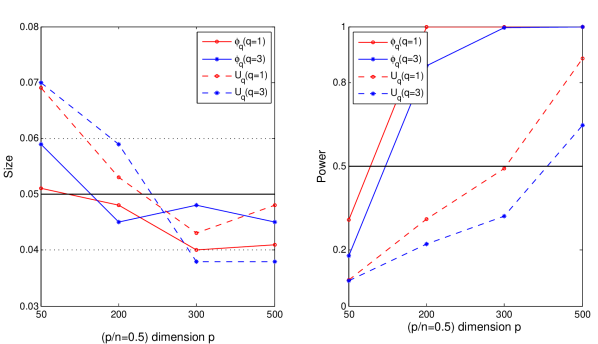
Figure 1: Sample plots of empirical sizes (left panel) from Table 1 (Scenario II with $c_{n}=0.5$) and empirical powers (right panel) from Table 2 (Scenario III with $c_{n}=0.5$).

In Table 2, we compare the power of the two tests. Our test $\phi_{q}$ displays a generally much higher power than the multi-lag-$q$ John’s test $U_{q}$, especially when the dimensions $(p,n)$ become larger. On the other hand, both tests have slightly lower power under the Non-Gaussian distribution than under the Gaussian distribution, which is consistent with the previous observation that the two tests become more conservative with Non-Gaussian populations. A sample display of these powers is given in Figure 1 (right panel).

To further explore the powers of the two tests, we varied the AR coefficient $a$ in Scenario (III) and (IV) from -0.1 to 0.1 ($a=0$ corresponds to testing size). Smaller values of the AR(1) coefficient $a$ are used here leading to a more difficult testing problem and a generally decreased power for both tests. Three dimensional settings are considered with $p/n\in\{0.1,0.5,1.5\}$ while the sample size is fixed as $n=600$. The number of independent replications is still 2000 in each case. Results for Scenario (III) and (IV) are plotted in Figure 1. This Figure further consolidates that our test $\phi_{q}$ dominates $U_{q}$ under all tested scenarios. A nonnegligible increase in the testing power of both test statistics as the dimension $p$ becomes larger sheds more light on the blessings of high dimensionality. Still both tests are more conservative with Non-Gaussian population distribution than with Gaussian distribution.

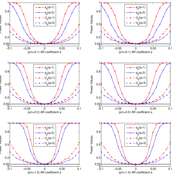
Figure 2: Empirical Powers for the two tests with varying AR coefficient $a$ from -0.1 to 0.1. Left panel: Scenario(III) for Gaussian Distribution. Right panel: Scenario(IV) for Gamma Distribution

3.2 Comparison to a permutation test

As many complex analytic tools are employed to derive the asymptotic null distributions of the test statistic $\phi_{q}$, it is natural to wonder about the performance of a “simple-minded” test procedure, namely the permutation test. Under the null hypothesis of white noise, since the sample vectors ${\bf x}_{1},\ldots,{\bf x}_{n}$ have an i.i.d. structure, one can permute these $n$ sample vectors say $B$ times to obtain an empirical upper 5% quantiles of the test statistic $\phi_{q}$. The null hypothesis will be rejected if the observed statistic $\phi_{q}$ from the original (non permuted) sample vectors ${\bf x}_{1},\ldots,{\bf x}_{n}$ is larger than this empirical quantile.

Data are generated following the spherical AR(1) process in Scenario (III) and (IV) to compare this straightforward test with our test statistic $\phi_{q}$. In order to compare the power performance of two tests, the AR coefficient $a$ takes different values, $a=[0,0.05,0.09,0.1]$ ($a=0$ corresponds to testing size). The sample size is fixed as $n=300$ yet data dimension $p$ varies. As for the permutation test, the permutation times is set as $B=500$. The nominal level is $\alpha=5\%$. Testing size and power of two tests are shown in Tables 3 and 4 based on 500 replicates for all $(p,n)$ configurations.

It can be seen that the sizes of both tests are well controlled. As for their power, our test offers an acceptable level while the permutation test consistently performs better in the tested cases. However, the permutation test is extremely time consuming compared to our test. For instance, to run one set of $(p,n)=(150,300)$ combination for 500 replicates, it takes only 25 seconds with our test, while almost 3 hours for the permutation test with permutation times $B=500$. Particularly the computation time increases greatly when the sample size $n$ grows. Therefore, our test statistic $\phi_{q}$ provides a very competitive choice for testing high dimensional white noise while the classical permutation test is simpler, more powerful though much slower.

4 Proofs of the main theorems

4.1 Proof of Theorem 2.1

The general strategy for our main Theorem 2.1 follows the methods advocated in Bai and Silverstein (2004), with its most recent update in Zheng et al. (2017b). However, as we are dealing with several random matrices simultaneously, all the technical steps for the implementation of this strategy have to be carefully rewritten. They are presented in this section.

4.1.1 Sketch of the proof of Theorem 2.1

Let $v_{0}>0$ be arbitrary, $x_{r}$ be any number greater than the right end point of interval (2.5), and $x_{l}$ be any negative number if the left end point of (2.5) is zero, otherwise choose $x_{l}\in(0,\liminf_{p\rightarrow\infty}\lambda_{\min}^{{\bf T}}(1-\sqrt{c})^{2})$. Define a contour $\mathcal{C}$ as

$$\mathcal{C}=\{x+iv:x\in\{x_{r},x_{l}\},v\in[-v_{0},v_{0}]\}\cup\mathcal{C}_{u}\ \text{with}\ \mathcal{C}_{u}=\{x\pm iv_{0}:x\in[x_{l},x_{r}]\},$$ (4.1)

and let $\mathcal{C}_{n}=\mathcal{C}_{u}\cup\{x\pm iv:x\in\{x_{l},x_{r}\},v\in[n^{-1}\varepsilon_{n},v_{0}]\}$ with $\varepsilon_{n}\geq n^{-\alpha}$ for some $\alpha\in(0,1)$. By definition, the contour $\mathcal{C}$ encloses a rectangular region in the complex plane, which contains the union of the support sets of all the LSDs $F^{c,H_{r}}$, $1\leq r\leq R$. As a regularized version of $\mathcal{C}$, $\mathcal{C}_{n}$ excludes a small segment near the real line.

Let $m_{nr}(z)$, $\underline{m}_{nr}(z)$, $m_{nr}^{0}(z)$, $\underline{m}_{nr}^{0}(z)$ be the Stieltjes transforms of $F_{nr}$, $\underline{F}_{nr}$, $F^{c_{n},H_{nr}}$, and $\underline{F}^{c_{n},H_{nr}}$, respectively, where $F_{nr}$ is the ESD of ${\bf B}_{nr}$, $F^{c_{n},H_{nr}}$ is the LSD defined in Remark 1, $F$ and $\underline{F}$ are linked by the equation $\underline{F}=(1-c_{n})\delta_{0}+c_{n}F$. A major task of proving Theorem 2.1 is to study the convergence of the empirical process

$$M_{nr}(z):=p[m_{nr}(z)-m_{nr}^{0}(z)]=n[\underline{m}_{nr}(z)-\underline{m}_{nr}^{0}(z)].$$

To this end, we need to truncate $M_{nr}(z)$ as

$$\widehat{M}_{nr}(z)=\begin{cases}M_{nr}(z)&z\in\mathcal{C}_{n},\\ M_{nr}(x+in^{-1}\varepsilon_{n})&x\in\{x_{l},x_{r}\}\quad\text{and}\quad v\in[0,n^{-1}\varepsilon_{n}],\\ M_{nr}(x-in^{-1}\varepsilon_{n})&x\in\{x_{l},x_{r}\}\quad\text{and}\quad v\in[-n^{-1}\varepsilon_{n},0],\end{cases}$$

which agrees to $M_{nr}(z)$ on $\mathcal{C}_{n}$. This truncation is essential when proving the tightness $\widehat{M}_{nr}(z)$ on $\mathcal{C}$. Write

$$\widehat{{\bf M}}_{n}(z)=\left(\widehat{M}_{n1}(z),\ldots,\widehat{M}_{nR}(z)\right),$$

we will establish its convergence as stated in the following lemma.

Lemma 4.1.

Under Assumptions (a)-(f), $\widehat{\bf M}_{n}(\cdot)$ converges weakly to a Gaussian process ${}{{\bf M}{}{(\cdot)}}=(M_{1},\ldots,M_{R})(\cdot)$ on ${\mathcal{C}}$. The mean function is

$${\rm E}M_{r}(z)=\frac{\alpha_{x}g_{1}(z)}{(1-g_{2}(z))(1-\alpha_{x}g_{2}(z))}+\frac{\beta_{x}g_{1}(z)}{1-g_{2}(z)},$$

where

$$g_{1}(z)=\int\frac{c\underline{m}_{r}^{3}(z)t^{2}}{(1+t\underline{m}_{r}(z))^{3}}dH_{r}(t)\quad\text{and}\quad g_{2}(z)=\int\frac{c\underline{m}_{r}^{2}(z)t^{2}}{(1+t\underline{m}_{r}(z))^{2}}dH_{r}(t).$$

The covariance function is

$${\rm Cov}(M_{r}(z_{1}),M_{s}(z_{2}))=-\frac{\partial^{2}}{\partial z_{1}\partial z_{2}}\left[\log(1-a(z_{1},z_{2}))+\log(1-\alpha_{x}{}{a(z_{1},z_{2})})-\beta_{x}a(z_{1},z_{2})\right]$$

where

$$a(z_{1},z_{2})=c\iint\frac{t_{1}t_{2}\underline{m}_{r}(z_{1})\underline{m}_{s}(z_{2})}{(1+t_{1}\underline{m}_{r}(z_{1}))(1+t_{2}\underline{m}_{s}(z_{2}))}dH_{rs}(t_{1},t_{2}).$$

From this lemma, Theorem 2.1 follows by similar arguments on Pages 562 and 563 in Bai and Silverstein (2004).

4.1.2 Proof of Lemma 4.1

Following closely the steps of truncation, centralization and rescaling in Appendix B of Zheng et al. (2017b), one may find that it is sufficient to prove this lemma under the assumption that

$$|x_{ij}|<\frac{\eta_{n}\sqrt{n}}{\max_{1\leq r\leq R}\{\|{\bf q}_{ir}\|\}},$$ (4.2)

where the constant $\eta_{n}\to 0$ as $n\to\infty$.

Write for $r\in\{1,\ldots,R\}$ and $z\in{\mathcal{C}}_{n}$,

$$M_{nr}(z) = p[m_{nr}(z)-{\rm E}m_{nr}(z)]+p[{\rm E}m_{nr}(z)-m_{nr}^{0}(z)]$$

$$:= M_{nr}^{1}(z)+M_{nr}^{2}(z).$$

The Lemma can be proved by verifying three conditions (Bai and Silverstein, 2004):

• Condition 1: Finite dimensional convergence of $M_{n}^{1}(z)$ in distribution;

• Condition 2: Tightness of $M_{n}^{1}(z)$ on $\mathcal{C}_{n}$;

• Condition 3: Convergence of $M_{n}^{2}(z)$.

Since the second and third conditions can be obtained directly from Lemma 5.1 in Zheng et al. (2017b), we only consider the first one by showing that, for any $W\times R$ complex numbers $z_{11},\ldots,z_{WR}$, the random vector $(M_{nr}^{1}(z_{jr}))_{1\leq j\leq W,1\leq r\leq R}$ converges to a Gaussian vector. Without loss of generality, we assume $\max\{\|{\bf Q}_{r}\|\}\leq 1$. We will also denote by $K$ any constants appearing in inequalities and $K$ may take on different values for different expressions.

With the notation ${\bf r}_{jr}=(1/\sqrt{n}){\bf Q}_{r}{\bf x}_{j}$, we define some quantities:

$${\bf D}_{r}(z)={\bf B}_{nr}-z{\bf I},\ {\bf D}_{jr}(z)={\bf D}_{r}(z)-{\bf r}_{jr}{\bf r}_{jr}^{*},\ {\bf D}_{ijr}(z)={\bf D}_{r}(z)-{\bf r}_{ir}{\bf r}_{ir}^{*}-{\bf r}_{jr}{\bf r}_{jr}^{*},$$

$${\epsilon}_{jr}(z)={\bf r}_{jr}^{*}{\bf D}^{-1}_{jr}(z){\bf r}_{jr}-n^{-1}{\rm tr}{\bf T}_{nr}{\bf D}^{-1}_{jr}(z),$$

$$\delta_{jr}(z)={\bf r}_{jr}^{*}{\bf D}^{-2}_{jr}(z){\bf r}_{jr}-n^{-1}{\rm tr}{\bf T}_{nr}{\bf D}^{-2}_{jr}(z),$$

$$\beta_{jr}(z)=\frac{1}{1+{\bf r}_{jr}^{*}{\bf D}_{jr}^{-1}(z){\bf r}_{jr}},\ \beta_{ijr}(z)=\frac{1}{1+{\bf r}_{ir}^{*}{\bf D}_{ijr}^{-1}(z){\bf r}_{ir}},\ \bar{\beta}_{jr}(z)=\frac{1}{1+n^{-1}{\rm tr}{\bf T}_{nr}{\bf D}_{jr}^{-1}(z)},$$

$$b_{nr}(z)=\frac{1}{1+n^{-1}{\rm E}{\rm tr}{\bf T}_{nr}{\bf D}_{r}^{-1}(z)},\ b_{12r}(z)=\frac{1}{1+n^{-1}{\rm E}{\rm tr}{\bf T}_{nr}{\bf D}_{12r}^{-1}(z)},$$

which will be frequently used in the sequel. Note that quantities in the last two rows are all bounded in absolute value by $|z|/\Im(z)$.

By martingale difference decomposition, the process $M_{nr}^{1}(z)$ can be expressed as

$$p[m_{nr}(z)-{\rm E}m_{nr}(z)]= ~{}{\rm tr}[{\bf D}_{r}^{-1}(z)-{\rm E}{\bf D}_{r}^{-1}(z)]$$

$$= ~{}\sum_{j=1}^{n}{\rm tr}{\rm E}_{j}[{\bf D}_{r}^{-1}(z)-{\bf D}^{-1}_{jr}(z)]-{\rm tr}{\rm E}_{j-1}[{\bf D}_{r}^{-1}(z)-{\bf D}^{-1}_{jr}(z)]$$

$$= ~{}-\sum_{j=1}^{n}({\rm E}_{j}-{\rm E}_{j-1})\beta_{jr}(z){\bf r}_{jr}^{*}{\bf D}^{-2}_{jr}(z){\bf r}_{jr}$$

$$= ~{}-\frac{d}{dz}{\sum\limits_{j=1}^{n}}({\rm E}_{j}-{\rm E}_{j-1})\log\beta_{jr}(z)$$

$$= ~{}\frac{d}{dz}{\sum\limits_{j=1}^{n}}({\rm E}_{j}-{\rm E}_{j-1})\log\big{(}1+{\epsilon}_{jr}(z)\bar{\beta}_{jr}(z)\big{)},$$

where the third equality is from the identity ${\bf D}^{-1}_{r}(z)={\bf D}_{jr}^{-1}(z)-{\bf D}_{jr}^{-1}(z){\bf r}_{jr}{\bf r}_{jr}^{*}{\bf D}_{jr}^{-1}(z)\beta_{jr}(z)$ and the last one is obtained using the identity $\beta_{jr}(z)=\bar{\beta}_{jr}(z)[1+\bar{\beta}_{jr}(z){\epsilon}_{jr}(z)]^{-1}$. We next show that

$$\frac{d}{dz}{\sum\limits_{j=1}^{n}}({\rm E}_{j}-{\rm E}_{j-1})\log\big{(}1+{\epsilon}_{jr}(z)\bar{\beta}_{jr}(z)\big{)}-\frac{d}{dz}{\sum\limits_{j=1}^{n}}({\rm E}_{j}-{\rm E}_{j-1}){\epsilon}_{jr}(z)\bar{\beta}_{jr}(z)=o_{p}(1).$$

Considering the second moment of the above difference, by the Cauchy integral formula, one may get

$$~{}{\rm E}\left|\frac{d}{dz}{\sum\limits_{j=1}^{n}}({\rm E}_{j}-{\rm E}_{j-1})\big{[}\log\big{(}1+{\epsilon}_{jr}(z)\bar{\beta}_{jr}(z)\big{)}-{\epsilon}_{jr}(z)\bar{\beta}_{jr}(z)\big{]}\right|^{2}$$

$$= ~{}{\rm E}\left|{\sum\limits_{j=1}^{n}}\frac{1}{2\pi{\bf i}}\oint_{|\zeta-z|=v/2}\frac{\big{[}\log\big{(}1+{\epsilon}_{jr}(\zeta)\bar{\beta}_{jr}(\zeta)\big{)}-{\epsilon}_{jr}(\zeta)\bar{\beta}_{jr}(\zeta)\big{]}}{(z-\zeta)^{2}}d\zeta\right|^{2}$$

$$\leq ~{}\frac{K}{\pi^{2}v^{4}}{\sum\limits_{j=1}^{n}}\oint_{|\zeta-z|=v/2}{\rm E}|{\epsilon}_{jr}(\zeta)\bar{\beta}_{jr}(\zeta)|^{4}|d\zeta|.$$ (4.3)

From Lemma A.1 and the truncation in (4.2), we have

$${\rm E}|{\epsilon}_{jr}(\zeta)|^{4}\leq ~{}\frac{K}{n^{4}}\bigg{\{}{\rm E}\left[{\rm tr}{\bf T}_{nr}{\bf D}_{jr}^{-1}(\zeta){\bf T}_{nr}{\bf D}_{jr}^{-1}(\bar{\zeta})\right]^{2}+\sum_{i=1}^{k}{\rm E}|x_{ij}|^{8}{\rm E}|{\bf q}_{ir}^{\top}{\bf D}_{jr}^{-1}(\zeta){\bf q}_{ir}|^{4}\bigg{\}}$$

$$\leq ~{}Kn^{-2}+K\eta_{n}^{4}n^{-1},$$

by which the right hand side of (4.3) tends to zero. Therefore, we need only to consider the limiting distribution of

$$\frac{d}{dz}{\sum\limits_{j=1}^{n}}({\rm E}_{j}-{\rm E}_{j-1}){\epsilon}_{jr}(z)\bar{\beta}_{jr}(z)=\frac{d}{dz}{\sum\limits_{j=1}^{n}}{\rm E}_{j}{\epsilon}_{jr}(z)\bar{\beta}_{jr}(z)$$ (4.4)

in finite dimensional situations. To verify the Lyapunov condition, one can show that

$${\sum\limits_{j=1}^{n}}{\rm E}\left|({\rm E}_{j}-{\rm E}_{j-1})\frac{d}{dz}{\epsilon}_{jr}(z)\bar{\beta}_{jr}(z)\right|^{2}I\left(\left|({\rm E}_{j}-{\rm E}_{j-1})\frac{d}{dz}{\epsilon}_{jr}(z)\bar{\beta}_{jr}(z)\right|\geq\epsilon\right)$$

$$\leq \frac{1}{\epsilon^{2}}{\sum\limits_{j=1}^{n}}{\rm E}\Big{|}{\rm E}_{j}\frac{d}{dz}{\epsilon}_{jr}(z)\bar{\beta}_{jr}(z)\Big{|}^{4}\to 0,$$

where the convergence is again from Lemma A.1 and (4.2). Hence, from the martingale (Billingsley, 1995, Theorem 35.12), the random vector $(M_{nr}^{1}(z_{jr}))$ will tend to a Gaussian vector $(M_{r}(z_{jr}))$ with covariance function

$${\rm Cov}(M_{r}(z_{1}),M_{s}(z_{2}))=\lim_{n\to\infty}{\sum\limits_{j=1}^{n}}{\rm E}_{j-1}\left({\rm E}_{j}\frac{\partial}{\partial z_{1}}{\epsilon}_{jr}(z_{1})\bar{\beta}_{jr}(z_{1})\cdot{\rm E}_{j}\frac{\partial}{\partial z_{2}}{\epsilon}_{js}(z_{2})\bar{\beta}_{js}(z_{2})\right).$$ (4.5)

We note that the referenced martingale CLT applies also to multidimensional martingale by considering arbitrary linear combination of its components.

Using the same approach of Bai and Silverstein (2004) on Page 571, one may replace $\bar{\beta}_{jr}(z)$ by $b_{nr}(z)$. Then, by (1.15) of Bai and Silverstein (2004), we have

$$\Gamma_{nrs}(z_{1},z_{2}){}{:=} \sum_{j=1}^{n}b_{nr}(z_{1})b_{ns}(z_{2}){\rm E}_{j-1}[{\rm E}_{j}\epsilon_{jr}(z_{1}){\rm E}_{j}\epsilon_{js}(z_{2})]$$

$$= ~{}\frac{1}{n^{2}}\sum_{j=1}^{n}b_{nr}(z_{1})b_{ns}(z_{2})\Bigg{[}{\rm tr}{\rm E}_{j}{\bf Q}_{r}^{\top}{\bf D}_{jr}^{-1}(z_{1}){\bf Q}_{r}{\rm E}_{j}{\bf Q}_{s}^{\top}{}{{\bf D}_{js}^{-1}}(z_{2}){\bf Q}_{s}$$

$$\quad\quad\quad\quad\quad\quad\quad\quad\quad+\alpha_{x}{\rm tr}{\rm E}_{j}{\bf Q}_{r}^{\top}{\bf D}_{jr}^{-1}(z_{1}){\bf Q}_{r}{\rm E}_{j}{\bf Q}_{s}^{\top}{}{{\bf D}_{js}^{-1}}(z_{2}){\bf Q}_{s}$$

$$\quad\quad\quad\quad\quad\quad\quad\quad\quad+\beta_{x}\sum_{i=1}^{k}{\bf q}_{ir}^{\top}{\rm E}_{j}{\bf D}_{jr}^{-1}(z_{1}){\bf q}_{ir}{\bf q}_{is}^{\top}{\rm E}_{j}{\bf D}_{js}^{-1}(z_{2}){\bf q}_{is}\Bigg{]}$$

$$:=\Gamma_{1}+\alpha_{x}\Gamma_{2}+\beta_{x}\Gamma_{3},$$ (4.6)

where $\alpha_{x}=|Ex_{11}^{2}|^{2}$ and $\beta_{x}=E|x_{11}^{4}|-{}{|Ex_{11}^{2}|^{2}}-2$.

Now we derive the limit of the first term in (4.6). The means is to replace ${\bf D}_{jr}^{-1}(z)$ (and similarly ${\bf D}_{js}^{-1}(z)$) by a proper nonrandom matrix. For this, we introduce such a one

$${\bf L}_{r}(z)=zI-\frac{n-1}{n}b_{12r}(z){\bf T}_{nr},$$

whose inverse spectral norm is bounded, that is,

$$||{\bf L}_{r}(z)||^{-1}\leq\frac{|b_{12r}^{-1}(z)|}{\Im(zb_{12r}^{-1}(z))}\leq\frac{1+p/(nv)}{v}.$$ (4.7)

We will show that the major part of ${\bf D}_{jr}^{-1}(z)$ is just $-{\bf L}_{r}^{-1}(z)$. From the identity ${\bf r}_{ir}^{*}{\bf D}_{jr}^{-1}(z)=\beta_{ijr}(z){\bf r}_{ir}^{*}{\bf D}_{ijr}^{-1}(z)$, we get

$${\bf D}_{jr}^{-1}(z)+{\bf L}_{r}^{-1}(z)= ~{}{\bf L}_{r}^{-1}(z)\left({\bf D}_{jr}(z)+{\bf L}_{r}(z)\right){\bf D}_{jr}^{-1}(z)$$

$$= ~{}{\bf L}_{r}^{-1}(z)\left(\sum_{i\neq j}{\bf r}_{ir}{\bf r}_{ir}^{*}-\frac{n-1}{n}b_{12r}(z){\bf T}_{nr}\right){\bf D}_{jr}^{-1}(z)$$

$$= ~{}{\bf L}_{r}^{-1}(z)\left(\sum_{i\neq j}\beta_{ijr}(z){\bf r}_{ir}{\bf r}_{ir}^{*}{\bf D}_{ijr}^{-1}(z)-\frac{n-1}{n}b_{12r}(z){\bf T}_{nr}{\bf D}_{jr}^{-1}(z)\right)$$

$$= ~{}b_{12r}(z){\bf R}_{1r}(z)+{\bf R}_{2r}(z)+{\bf R}_{3r}(z),$$ (4.8)

where

$${\bf R}_{1r}(z)=\sum_{i\neq j}{\bf L}_{r}^{-1}(z)({\bf r}_{ir}{\bf r}_{ir}^{*}-n^{-1}{\bf T}_{nr}){\bf D}_{ijr}^{-1}(z),$$

$${\bf R}_{2r}(z)=\sum_{i\neq j}(\beta_{ijr}(z)-b_{12r}(z)){\bf L}_{r}^{-1}(z){\bf r}_{ir}{\bf r}_{ir}^{*}{\bf D}_{ijr}^{-1}(z),$$

$${\bf R}_{3r}(z)=n^{-1}b_{12r}(z){\bf L}_{r}^{-1}(z){\bf T}_{nr}\sum_{i\neq j}\left({\bf D}_{ijr}^{-1}(z)-{}{{\bf D}_{jr}^{-1}(z)}\right).$$

From this decomposition, after substituting $-{\bf L}_{r}^{-1}(z)$ for ${\bf D}_{jr}^{-1}(z)$ in the first term in (4.6), there are three remaining quantities. Let’s check which one (or ones) of them can be omitted. From Lemma A.3, (4.7), and (4.3) of Bai and Silverstein (1998), for any $p\times p$ matrix ${\bf M}$, we have

$${\rm E}|{\rm tr}{\bf R}_{2r}(z){\bf M}|\leq ~{}n{\rm E}^{1/2}(|\beta_{12r}(z)-b_{12r}(z)|^{2}){\rm E}^{1/2}\bigg{|}{\bf r}_{1r}^{*}{\bf D}_{12r}^{-1}{\bf M}{\bf L}_{r}^{-1}(z){\bf r}_{1r}\bigg{|}^{2}$$

$$\leq ~{}n^{1/2}K|||{\bf M}|||\frac{|z|^{2}(1+p/(nv))}{v^{5}},$$ (4.9)

where $|||{\bf M}|||$ denotes a nonrandom bound on the spectral norm of ${\bf M}$. From Lemma A.2,

$$|{\rm tr}{\bf R}_{3r}(z){\bf M}|\leq ~{}|||{\bf M}|||\frac{|z|(1+p/(nv))}{v^{3}}.$$ (4.10)

Again from Lemma A.3 and (4.7), for nonrandom ${\bf M}$,

$${\rm E}|{\rm tr}{\bf R}_{1r}(z){\bf M}|\leq ~{}n{\rm E}^{1/2}|{\bf r}_{ir}^{*}{\bf D}_{ijr}^{-1}(z){\bf M}{\bf L}_{r}^{-1}(z){\bf r}_{ir}-n^{-1}{\rm tr}{\bf T}_{nr}{\bf D}_{ijr}^{-1}(z){\bf M}{\bf L}_{r}^{-1}(z)|^{2}$$

$$\leq ~{}n^{1/2}K||{\bf M}||\frac{(1+p/(nv))}{v^{2}}.$$ (4.11)

Therefore, quantities containing ${\bf R}_{2r}(z)$ and ${\bf R}_{3r}(z)$ are both negligible. For the quantity involving ${\bf R}_{1r}(z)$, applying the identity ${\bf D}^{-1}_{js}(z)={\bf D}_{ijs}^{-1}(z)-{\bf D}_{ijs}^{-1}(z){\bf r}_{js}{\bf r}_{js}^{*}{\bf D}_{ijs}^{-1}(z)\beta_{ijs}(z)$, it can be divided into three parts, that is,

$${\rm tr}{\bf Q}_{r}^{\top}{\rm E}_{j}({\bf R}_{1r}(z_{1})){\bf Q}_{r}{\bf Q}_{s}^{\top}{\bf D}_{js}^{-1}(z_{2}){\bf Q}_{s}=R_{11}(z_{1},z_{2})+R_{12}(z_{1},z_{2})+R_{13}(z_{1},z_{2}),$$ (4.12)

where

$$R_{11}(z_{1},z_{2}) =-\sum_{i<j}\beta_{ijs}(z_{2}){\bf r}_{ir}^{*}{\rm E}_{j}({\bf D}_{ijr}^{-1}(z_{1})){\bf Q}_{r}{\bf Q}_{s}^{\top}{\bf D}_{ijs}^{-1}(z_{2}){\bf r}_{is}{\bf r}_{is}^{*}{\bf D}_{ijs}^{-1}(z_{2}){\bf Q}_{s}{\bf Q}_{r}^{\top}{\bf L}_{r}^{-1}(z_{1}){\bf r}_{ir},$$

$$R_{12}(z_{1},z_{2}) =-{\rm tr}\sum_{i<j}{\bf L}_{r}^{-1}(z_{1})n^{-1}{\bf T}_{nr}{\rm E}_{j}({\bf D}_{ijr}^{-1}(z_{1})){\bf Q}_{r}{\bf Q}_{s}^{\top}({\bf D}_{js}^{-1}(z_{2})-{\bf D}_{ijs}^{-1}(z_{2})){\bf Q}_{s}{\bf Q}_{r}^{\top},$$

$$R_{13}(z_{1},z_{2}) ={\rm tr}\sum_{i<j}{\bf L}_{r}^{-1}(z_{1})({\bf r}_{ir}{\bf r}_{ir}^{*}-n^{-1}{\bf T}_{nr}){\rm E}_{j}({\bf D}_{ijr}^{-1}(z_{1})){\bf Q}_{r}{\bf Q}_{s}^{\top}{\bf D}_{ijs}^{-1}(z_{2}){\bf Q}_{s}{\bf Q}_{r}^{\top}.$$

From Lemma A.2 and (4.7) we get $|R_{12}(z_{1},z_{2})|\leq(1+p/(nv_{0}))/v_{0}^{3}$, and similar to (4.9), ${\rm E}|R_{13}(z_{1},z_{2})|\leq n^{1/2}(1+p/(nv_{0}))/v_{0}^{3}$. Thus these two parts are trivial. We then turn to dealing with $R_{11}(z_{1},z_{2})$. Using Lemma A.1, Lemma A.3, and (4.3) of Bai and Silverstein (1998) we get, for $i<j$,

$${\rm E}\bigg{|}\beta_{ijs}(z_{2}){\bf r}_{ir}^{*}{\rm E}_{j}({\bf D}_{ijr}^{-1}(z_{1})){\bf Q}_{r}{\bf Q}_{s}^{\top}{\bf D}_{ijs}^{-1}(z_{2}){\bf r}_{is}{\bf r}_{is}^{*}{\bf D}_{ijs}^{-1}(z_{2}){\bf Q}_{s}{\bf Q}_{r}^{\top}{\bf L}_{r}^{-1}(z_{1}){\bf r}_{ir}$$

$$-b_{12s}(z_{2})n^{-2}{\rm tr}\left({\rm E}_{j}({\bf D}_{ijr}^{-1}(z_{1})){\bf Q}_{r}{\bf Q}_{s}^{\top}{\bf D}_{ijs}^{-1}(z_{2}){\bf Q}_{s}{\bf Q}_{r}^{\top}\right){\rm tr}\left({\bf D}_{ijs}^{-1}(z_{2}){\bf Q}_{s}{\bf Q}_{r}^{\top}{\bf L}_{r}^{-1}(z_{1}){\bf Q}_{r}{\bf Q}_{s}^{\top}\}\right)\bigg{|}$$

$$\leq Kn^{-1/2}.$$

So we may simplify $R_{11}(z_{1},z_{2})$ by replacing $\beta_{ijs}(z_{2})$ with $b_{12s}(z_{2})$ and remove the random parts of ${\bf r}_{ir}$ and ${\bf r}_{is}$. By Lemma A.2, we have

$$\bigg{|}{\rm tr}\left({\rm E}_{j}({\bf D}_{ijr}^{-1}(z_{1})){\bf Q}_{r}{\bf Q}_{s}^{\top}{\bf D}_{ijs}^{-1}(z_{2}){\bf Q}_{s}{\bf Q}_{r}^{\top}\right){\rm tr}\left({\bf D}_{ijs}^{-1}(z_{2}){\bf Q}_{s}{\bf Q}_{r}^{\top}{\bf L}_{r}^{-1}(z_{1}){\bf Q}_{r}{\bf Q}_{s}^{\top}\}\right)$$

$$-{\rm tr}\left({\rm E}_{j}({}{{\bf D}_{jr}^{-1}}(z_{1})){\bf Q}_{r}{\bf Q}_{s}^{\top}{\bf D}_{js}^{-1}(z_{2}){\bf Q}_{s}{\bf Q}_{r}^{\top}\right){\rm tr}\left({\bf D}_{js}^{-1}(z_{2}){\bf Q}_{s}{\bf Q}_{r}^{\top}{\bf L}_{r}^{-1}(z_{1}){\bf Q}_{r}{\bf Q}_{s}^{\top}\}\right)\bigg{|}\leq Kn.$$

It implies that we may further replace ${\bf D}_{ijr}^{-1}(z_{1})$ and ${\bf D}_{ijs}^{-1}(z_{2})$ in $R_{11}(z_{1},z_{2})$ with ${\bf D}_{jr}^{-1}(z_{1})$ and ${\bf D}_{js}^{-1}(z_{2})$, respectively, which yields

$${\rm E}\bigg{|}R_{11}(z_{1},z_{2})$$

$$+\frac{j-1}{n^{2}}b_{12s}(z_{2}){\rm tr}\left({\bf Q}_{r}^{\top}{\rm E}_{j}({\bf D}_{jr}^{-1}(z_{1})){\bf Q}_{r}{\bf Q}_{s}^{\top}{\bf D}_{js}^{-1}(z_{2}){\bf Q}_{s}\right){\rm tr}\left({\bf Q}_{s}^{\top}{\bf D}_{js}^{-1}(z_{2}){\bf Q}_{s}{\bf Q}_{r}^{\top}{\bf L}_{r}^{-1}(z_{1}){\bf Q}_{r}\right)\bigg{|}$$

$$\leq Kn^{1/2}.$$ (4.13)

Integrating the results in (4.8)-(4.13), we obtain

$${\rm tr}\left({\bf Q}_{r}^{\top}{\rm E}_{j}({\bf D}_{jr}^{-1}(z_{1})){\bf Q}_{r}{\bf Q}_{s}^{\top}{\bf D}_{js}^{-1}(z_{2}){\bf Q}_{s}\right)$$ (4.14)

$$\times\left(1+\frac{j-1}{n^{2}}b_{12r}(z_{1})b_{12s}(z_{2}){\rm tr}\left({\bf Q}_{s}^{\top}{\bf D}_{js}^{-1}(z_{2}){\bf Q}_{s}{\bf Q}_{r}^{\top}{\bf L}_{r}^{-1}(z_{1}){\bf Q}_{r}\right)\right)$$

$$= -{\rm tr}{\bf Q}_{r}^{\top}{\bf L}_{r}^{-1}(z_{1}){\bf Q}_{r}{\bf Q}_{s}^{\top}{\bf D}_{js}^{-1}(z_{2}){\bf Q}_{s}+R_{14}(z_{1},z_{2}),$$

where ${\rm E}|R_{14}(z_{1},z_{2})|\leq Kn^{1/2}$. Furthermore, from this and (4.8)-(4.11), we may substitute for the second and third ${\bf D}_{js}^{-1}(z_{2})$ in (4.14) with $-{\bf L}_{s}^{-1}(z_{2})$ and then get

$${\rm tr}\left({\bf Q}_{r}^{\top}{\rm E}_{j}({\bf D}_{jr}^{-1}(z_{1})){\bf Q}_{r}{\bf Q}_{s}^{\top}{\bf D}_{js}^{-1}(z_{2}){\bf Q}_{s}\right)$$ (4.15)

$$\times\left(1-\frac{j-1}{n^{2}}b_{12r}(z_{1})b_{12s}(z_{2}){\rm tr}\left({\bf Q}_{s}^{\top}{\bf L}_{s}^{-1}(z_{2}){\bf Q}_{s}{\bf Q}_{r}^{\top}{\bf L}_{r}^{-1}(z_{1}){\bf Q}_{r}\right)\right)$$

$$= {\rm tr}{\bf Q}_{r}^{\top}{\bf L}_{r}^{-1}(z_{1}){\bf Q}_{r}{\bf Q}_{s}^{\top}{\bf L}_{s}^{-1}(z_{2}){\bf Q}_{s}+R_{15}(z_{1},z_{2}),$$

where ${\rm E}|R_{15}(z_{1},z_{2})|\leq Kn^{1/2}$.

From Lemma A.2 and (4.3) of Bai and Silverstein (1998), we have

$$|b_{12r}(z)-b_{nr}(z)|\leq Kn^{-1}\quad\text{and}\quad|b_{nr}(z)-{\rm E}\beta_{1r}(z)|\leq Kn^{-1/2},$$

respectively. By (2.2) of Silverstein (1995) and discussions in Section 5 of Bai and Silverstein (1998), we have

$${\rm E}\beta_{1r}(z)=-z{\rm E}\underline{m}_{nr}(z)\quad\text{and}\quad|{\rm E}\underline{m}_{nr}(z)-\underline{m}_{nr}^{0}(z)|\leq Kn^{-1},$$

respectively. Therefore, we get

$$|b_{12r}(z)+z\underline{m}_{nr}^{0}(z)|\leq Kn^{-1/2}.$$ (4.16)

Combining this and (4.15), it follows that

$${\rm tr}\left({\bf Q}_{r}^{\top}{\rm E}_{j}({\bf D}_{jr}^{-1}(z_{1})){\bf Q}_{r}{\bf Q}_{s}^{\top}{\bf D}_{js}^{-1}(z_{2}){\bf Q}_{s}\right)\left(1-\frac{j-1}{n^{2}}\underline{m}_{nr}^{0}(z_{1})\underline{m}_{ns}^{0}(z_{2})\right.$$ (4.17)

$$\times{\rm tr}\left({\bf Q}_{s}^{\top}(I+\underline{m}_{ns}^{0}(z_{2}){\bf T}_{ns})^{-1}{\bf Q}_{s}{\bf Q}_{r}^{\top}(I+\underline{m}_{nr}^{0}(z_{1}){\bf T}_{nr})^{-1}{\bf Q}_{r}\right)\bigg{)}$$

$$= {\rm tr}\left({\bf Q}_{r}^{\top}{\rm E}_{j}({\bf D}_{jr}^{-1}(z_{1})){\bf Q}_{r}{\bf Q}_{s}^{\top}{\bf D}_{js}^{-1}(z_{2}){\bf Q}_{s}\right)\left(1-\frac{j-1}{n}c_{n}\underline{m}_{nr}^{0}(z_{1})\underline{m}_{ns}^{0}(z_{2})\right.$$

$$\times\int\int\frac{t_{1}t_{2}dH_{prs}(t_{1},t_{2})}{(1+t_{1}\underline{m}_{nr}^{0}(z_{1}))(1+t_{2}\underline{m}_{ns}^{0}(z_{2}))}\bigg{)}$$

$$= \frac{nc_{n}}{z_{1}z_{2}}\int\int\frac{t_{1}t_{2}dH_{prs}(t_{1},t_{2})}{(1+t_{1}\underline{m}_{nr}^{0}(z_{1}))(1+t_{2}\underline{m}_{ns}^{0}(z_{2}))}+R_{16}(z_{1},z_{2}),$$

where ${\rm E}|R_{16}(z_{1},z_{2})|\leq Kn^{1/2}$. Similar to the arguments in Bai and Silverstein (2004) (page 577), using (4.17) and letting

$$a_{n}(z_{1},z_{2})=c_{n}\underline{m}_{nr}^{0}(z_{1})\underline{m}_{ns}^{0}(z_{2})\int\int\frac{t_{1}t_{2}dH_{prs}(t_{1},t_{2})}{(1+t_{1}\underline{m}_{nr}^{0}(z_{1}))(1+t_{2}\underline{m}_{ns}^{0}(z_{2}))},$$

we get

$$\Gamma_{1}=\frac{1}{n}\sum_{j=1}^{n}\frac{a_{n}(z_{1},z_{2})}{1-((j-1)/n)a_{n}(z_{1},z_{2})}+o_{p}(1)\xrightarrow{i.p.}-\log(1-a(z_{1},z_{2})),$$ (4.18)

where

$$a(z_{1},z_{2})=c\underline{m}_{r}(z_{1})\underline{m}_{s}(z_{2})\int\int\frac{t_{1}t_{2}dH_{rs}(t_{1},t_{2})}{(1+t_{r}\underline{m}_{r}(z_{1}))(1+t_{s}\underline{m}_{s}(z_{2}))}.$$

Similar to the derivation of $\Gamma_{1}$, one can easily show that

$$\alpha_{x}\Gamma_{2}=\frac{1}{n}\sum_{j=1}^{n}\frac{\alpha_{x}a_{n}(z_{1},z_{2})}{1-\alpha_{x}((j-1)/n)a_{n}(z_{1},z_{2})}+o_{p}(1)\xrightarrow{i.p.}-\log(1-\alpha_{x}a(z_{1},z_{2})).$$ (4.19)

Considering the third term of (4.6), $\beta_{x}\Gamma_{3}$ with $\beta_{x}\neq 0$, from Assumption (e), the matrix ${\bf Q}_{r}^{\top}{\bf Q}_{r}$ is diagonal, so is ${\bf Q}_{r}^{\top}{\bf L}_{r}^{-1}{\bf Q}_{r}$. Using (4.8)-(4.11) and (4.16), we have

$$\beta_{x}\Gamma_{3}= ~{}\beta_{x}b_{nr}(z_{1})b_{ns}(z_{2})\frac{1}{n^{2}}\sum_{j=1}^{n}\sum\limits_{i=1}^{k}{\bf e}_{i}^{\top}{\bf Q}_{r}^{\top}{\rm E}_{j}({\bf D}_{jr}^{-1}(z_{1})){\bf Q}_{r}{\bf e}_{i}{\bf e}_{i}^{\top}{\bf Q}_{s}^{\top}{\rm E}_{j}({\bf D}_{js}^{-1}(z_{2})){\bf Q}_{s}{\bf e}_{i}$$

$$= ~{}\beta_{x}b_{nr}(z_{1})b_{ns}(z_{2})\frac{1}{n^{2}}\sum_{j=1}^{n}\sum\limits_{i=1}^{k}{\bf e}_{i}^{\top}{\bf Q}_{r}^{\top}{\bf L}_{r}^{-1}(z_{1}){\bf Q}_{r}{\bf e}_{i}{\bf e}_{i}^{\top}{\bf Q}_{s}^{\top}{\bf L}_{s}^{-1}(z_{2}){\bf Q}_{s}{\bf e}_{i}+o_{p}(1)$$

$$= ~{}\beta_{x}b_{nr}(z_{1})b_{ns}(z_{2})\frac{1}{n^{2}}\sum_{j=1}^{n}{\rm tr}\left({\bf Q}_{r}^{\top}{\bf L}_{r}^{-1}(z_{1}){\bf Q}_{r}{\bf Q}_{s}^{\top}{\bf L}_{s}^{-1}(z_{2}){\bf Q}_{s}\right)+o_{p}(1)$$

$$\xrightarrow{i.p.} ~{}\beta_{x}a(z_{1},z_{2}).$$ (4.20)

Collecting the results in (4.5), (4.18)-(4.20), we finally get the covariance function in the Lemma and the proof of this Lemma is completed.

4.2 Proof of Theorem 3.1

First we show that it is it is enough to establish the following claim: under the (classical) Marčenko-Pastur regime, i.e., $n\to\infty$, $p=p_{n}\to\infty$ such that $p/n\to c>0$, it holds that

$$\phi_{q,n}-\frac{q}{2}\xrightarrow{d}\mathcal{N}\left(0,s(c)\right),$$ (4.21)

where recall that $s(u)=q+u(\nu_{4}-1)(q^{2}+\frac{q}{2})$. Here we use $\phi_{q,n}$ for $\phi_{q}$ to signify the dependence in $n$. So assume this claim is true. Under the relaxed Marčenko-Pastur regime, the sequence $\{p_{n}/n\}$ is bounded below and above. For any subsequence $(p_{n_{k}},n_{k})_{k}$ of $(p_{n},n)$, we can extract a further subsequence $(p_{n_{k_{\ell}}},n_{k_{\ell}})_{\ell}$ such that the ratios $p_{n_{k_{\ell}}}/n_{k_{\ell}}$ converge to $\alpha>0$ when $\ell\to\infty$. On this subsequence, by Claim (4.21),

$$\phi_{q,n_{k_{\ell}}}-\frac{q}{2}\xrightarrow{d}\mathcal{N}\left(0,s(\alpha)\right),\quad\ell\to\infty.$$

By continuity of the function $u\to s(u)$, we have

$$s(p_{n_{k_{\ell}}}/n_{k_{\ell}})^{-1/2}\left(\phi_{q,n_{k_{\ell}}}-\frac{q}{2}\right)\xrightarrow{d}\mathcal{N}\left(0,1\right),\quad\ell\to\infty.$$

As this limit is independent of the subsequence and it holds for all such subsequences, the same limit holds for the whole sequence, that is,

$$s(p_{n}/n)^{-1/2}\left(\phi_{q,n}-\frac{q}{2}\right)\xrightarrow{d}\mathcal{N}\left(0,1\right),\quad\ell\to\infty.$$

The required asymptotic normality is thus established.

The remaining of the section is devoted to a proof of Claim (4.21) assuming $p/n\to c>0$. Define the banded Toeplitz matrix

$${\bf C}_{n,\tau}=\left(\begin{array}[]{ccccc}0&\cdots&\frac{1}{2}&\cdots&0\\ \vdots&\ddots&0&\frac{1}{2}&\vdots\\ \frac{1}{2}&0&\ddots&0&\frac{1}{2}\\ \vdots&\frac{1}{2}&0&\ddots&\vdots\\ 0&\cdots&\frac{1}{2}&\cdots&0\\ \end{array}\right)_{n\times n}$$

and

$$\widehat{{\bf N}}_{\tau}=\frac{1}{2p}\sum_{t=1+\tau}^{n}\left({\bf x}_{t}{\bf x}_{t-\tau}^{*}+{\bf x}_{t-\tau}{\bf x}_{t}^{*}\right)=\frac{1}{p}{\bf X}_{n}{\bf C}_{n,\tau}{\bf X}_{n}^{*}.$$

Define the associated Fourier series $f(\lambda)$ of the banded Toeplitz matrix ${\bf C}_{n,\tau}$ as

$$f(\lambda) =\lim_{n\rightarrow\infty}\sum_{k=-\tau}^{\tau}t_{k}e^{ik\lambda}=\frac{1}{2}\left(e^{i\tau\lambda}+e^{-i\tau\lambda}\right)=\cos(\tau\lambda),$$

where $t_{k}$ is entry on the $k$-diagonal of ${\bf C}_{n,\tau}$.

According to the fundamental eigenvalue distribution theorem of Szegö for Toeplitz forms, see Section 5.2 in Grenander and Szegö (1958) and Theorem 4.1 in Gray (2006), we can infer that

Lemma 4.2.

Suppose $\{l_{t},~{}t=1,\cdots,n\}$ are eigenvalues of ${\bf C}_{n,\tau}$ with Fourier series $f(\lambda)$, then

• For any positive integer $s$,

  $$\lim_{n\rightarrow\infty}\frac{1}{n}\sum_{t=1}^{n}l_{t}^{s}=\frac{1}{2\pi}\int_{0}^{2\pi}f(\lambda)^{s}\operatorname{d}\!{\lambda}=\frac{1}{2\pi}\int_{0}^{2\pi}\left(\cos(\tau\lambda)\right)^{s}\operatorname{d}\!{\lambda},$$

• For any continuous function on support of $\{l_{t},~{}t=1,\cdots,n\}$,

  $$\lim_{n\rightarrow\infty}\frac{1}{n}\sum_{t=1}^{n}F(l_{t})=\frac{1}{2\pi}\int_{0}^{2\pi}F\left(\cos(\tau\lambda)\right)\operatorname{d}\!{\lambda},$$

• Sequence $\left\{l_{t},~{}t=1,\cdots,n\right\}$ and

  $$\left\{\cos\left(\frac{2\pi\tau t}{n}\right),~{}t=1,\cdots,n\right\}$$

  are asymptotically equally distributed.

The limiting spectral distribution of ${\bf C}_{n,\tau}$ is also derived in Lemma 3.1 of Bai and Wang (2015), this useful lemma is stated as follows:

Lemma 4.3.

As $T\rightarrow\infty$, the ESD of ${\bf C}_{n,\tau}$ tends to $H$, which is an Arcsine distribution with density function

$$H^{\prime}(t)=\cfrac{1}{\pi\sqrt{1-t^{2}}},~{}t\in(-1,1).$$

Recall for the permutation matrices ${\bf D}_{1}$ and ${\bf D}_{\tau}={\bf D}_{1}^{\tau}$ defined in Introduction, it holds that

$${\bf D}_{1}{\bf D}_{1}^{\top}={\bf D}_{1}^{\top}{\bf D}_{1}={\bf D}_{\tau}{\bf D}_{\tau}^{\top}={\bf D}_{\tau}^{\top}{\bf D}_{\tau}={\bf I}_{n}.$$

Meanwhile, from the properties of Chebyshev polynomials, we can derive the following lemma.

Lemma 4.4.

• $\frac{1}{2}\left({\bf D}_{1}+{\bf D}_{1}^{\top}\right)$ has eigenvalue

  $$\left\{\cos\left(\frac{2\pi t}{n}\right),~{}t=1,\cdots,n\right\},$$

• $\frac{1}{2}\left({\bf D}_{\tau}+{\bf D}_{\tau}^{\top}\right)$ has eigenvalue

  $$\left\{T_{\tau}\left(\cos\left(\frac{2\pi t}{n}\right)\right),~{}t=1,\cdots,n\right\},$$

  where $T_{\tau}(\cdot)$ stands for the Chebyshev polynomial of order $\tau$.

• $\frac{1}{2}\left({\bf D}_{\tau}+{\bf D}_{\tau}^{\top}\right)$ shares the same asymptotic spectral distribution with ${\bf C}_{n,\tau}$ as $n\rightarrow\infty$.

Since

$$\widetilde{{\bf N}}_{\tau} =\frac{1}{2p}\sum_{t=1}^{n}\left({\bf x}_{t}{\bf x}_{t-\tau}^{*}+{\bf x}_{t-\tau}{\bf x}_{t}^{*}\right)$$

$$=\frac{1}{2p}\left({\bf x}_{1},\cdots,{\bf x}_{n}\right)\left(\sum_{\tau=1}^{q}\left({\bf D}_{\tau}+{\bf D}_{\tau}^{\top}\right)\right)\left({\bf x}_{1},\cdots,{\bf x}_{n}\right)^{*}$$

$$=\frac{1}{2p}{\bf X}_{n}\left(\sum_{\tau=1}^{q}\left({\bf D}_{\tau}+{\bf D}_{\tau}^{\top}\right)\right){\bf X}_{n}^{*},$$

here for $t\leq 0$, ${\bf x}_{t}={\bf x}_{n+t}$, by Lemmas 4.2 and 4.4, it doesn’t take too much effort to see that $\widetilde{{\bf N}}_{\tau}$ and $\widehat{{\bf N}}_{\tau}$ share the same limiting spectral distribution.

Consider the Stieltjes transform $\underline{m}_{\tau}(z)$ of the limiting spectral distribution of $\widetilde{{\bf N}}_{\tau}$, by implementing the Silverstein equation (2.2), we can infer that $\underline{m}_{\tau}(z)$ satisfies

$$z =-\frac{1}{\underline{m}_{\tau}(z)}+\frac{1}{c}\int\frac{t}{1+t\underline{m}_{\tau}(z)}dH_{\tau}(t)$$

$$=\frac{1}{\underline{m}_{\tau}(z)}\left(-1+\frac{1}{c}-\frac{1}{c\sqrt{1-\underline{m}_{\tau}^{2}(z)}}\right),$$

where $p/n\rightarrow c>0$ as $n\rightarrow\infty$, which coincides with the results in Bai and Wang (2015) and Li et al. (2016).

Note that our test statistic

$$\mathcal{L}_{q}=\sum_{\tau=1}^{q}\widetilde{L}_{\tau}=\sum_{\tau=1}^{q}\mathrm{Tr}(\widetilde{{\bf M}}_{\tau}\widetilde{{\bf M}}_{\tau}^{*})=\left(\frac{p}{n}\right)^{2}\sum_{\tau=1}^{q}\mathrm{Tr}(\widetilde{{\bf N}}_{\tau}\widetilde{{\bf N}}_{\tau}^{*}),$$

where $\widetilde{{\bf M}}_{\tau}=\frac{1}{2}\left(\widehat{{\bm{\Sigma}}}_{\tau}+\widehat{{\bm{\Sigma}}}_{\tau}^{*}\right)=\frac{1}{2n}\sum_{t=1}^{n}\left({\bf x}_{t}{\bf x}_{t-\tau}^{*}+{\bf x}_{t-\tau}{\bf x}_{t}^{*}\right)$, thus the asymptotic properties of $\widetilde{{\bf M}}_{\tau}$ can be inferred from those of $\widetilde{{\bf N}}_{\tau}$ since $\widetilde{{\bf M}}_{\tau}=\frac{p}{n}\widetilde{{\bf N}}_{\tau}$.

Actually in Li et al. (2016), the asymptotic behavior of the single-lag-$\tau$ test statistic $\widetilde{L}_{\tau}$ has already been thoroughly explored and characterized. Theorem 2.1 in Li et al. (2016) is stated as follows:

Lemma 4.5.

Let $\tau\geq 1$ be a fixed integer, and assume that

1. $\{z_{it},~{}i=1,\cdots,p,~{}t=1,\cdots,n\}$ are all independently distributed satisfying ${\rm E}z_{it}=0,~{}{\rm E}z_{it}^{2}=1,~{}{\rm E}z_{it}^{4}=\nu_{4}<\infty$;

2. (Marčenko-Pastur regime). The dimension $p$ and the sample size $n$ grow to infinity in a related way such that $c_{n}:=p/n\rightarrow c>0$.

Then in the simplest setting when ${\bf x}_{t}=\mathbf{z}_{t}$, the limiting distribution of the test statistic $\widetilde{L}_{\tau}$ is

$$\frac{n}{p}\widetilde{L}_{\tau}-\frac{p}{2}\xrightarrow{d}\mathcal{N}\left(\frac{1}{2},~{}1+\frac{3(\nu_{4}-1)}{2}c\right).$$

Now consider the multi-lag-$q$ test statistic $\mathcal{L}_{q}=\sum_{\tau=1}^{q}\widetilde{L}_{\tau}$, combining with Lemma 4.5, all we need is the joint distribution of any two different single-lag test statistic, i.e. $\left(\widetilde{L}_{r},\widetilde{L}_{s}\right),~{}1\leq r\neq s\leq q$.

For a given integer $q>0$, $1\leq r\neq s\leq q$, let $f_{r}(x)=f_{s}(x)=x^{2},$

$${\bf B}_{nr} =\frac{1}{2p}\left({\bf D}_{r}+{\bf D}_{r}^{\top}\right){\bf X}_{n}^{*}{\bf X}_{n},~{}B_{ns}=\frac{1}{2p}\left({\bf D}_{s}+{\bf D}_{s}^{\top}\right){\bf X}_{n}^{*}{\bf X}_{n},$$

$$\underline{{\bf B}}_{nr} =\widetilde{{\bf N}}_{r}=\frac{1}{2p}{\bf X}_{n}\left({\bf D}_{r}+{\bf D}_{r}^{\top}\right){\bf X}_{n}^{*},~{}\underline{B}_{ns}=\widetilde{{\bf N}}_{s}=\frac{1}{2p}{\bf X}_{n}\left({\bf D}_{s}+{\bf D}_{s}^{\top}\right){\bf X}_{n}^{*},$$

then both the LSDs of $\underline{{\bf B}}_{nr}$ and $\underline{{\bf B}}_{ns}$, i.e. $\underline{F}^{c,H_{r}},~{}\underline{F}^{c,H_{s}}$ have Stieltjes transform $\underline{m}_{r}(z)$ and $\underline{m}_{s}(z)$ satisfying the equation

$$z=\frac{1}{\underline{m}(z)}\left(-1+\frac{1}{c}-\frac{1}{c\sqrt{1-\underline{m}^{2}(z)}}\right).$$

Meanwhile,

$$\mathrm{Tr}(\widetilde{{\bf N}}_{r}\widetilde{{\bf N}}_{r}^{*})=\int f_{r}(x)\operatorname{d}\!{F}_{nr}(x),~{}\mathrm{Tr}(\widetilde{{\bf N}}_{s}\widetilde{{\bf N}}_{s}^{*})=\int f_{s}(x)\operatorname{d}\!{F}_{ns}(x).$$

where $F_{nr}$ and $F_{ns}$ are the ESDs of ${\bf B}_{nr}$ and ${\bf B}_{ns}$. Thus, by directly implementing our joint CLT for linear spectral statistics of the sample covariance matrices, i.e. Theorem 2.1, we can derive the joint distribution of $\left(\widetilde{L}_{1},\cdots,\widetilde{L}_{q}\right)$ or any pair of $\left(\widetilde{L}_{r},\widetilde{L}_{s}\right),~{}1\leq r\neq s\leq q$. Precisely, the covariance function in Theorem 2.1 for the present case can be calculated to be

$${\rm Cov}\left(X_{f_{r}},X_{f_{s}}\right)=\left\{\begin{array}[]{ll}\frac{1+\frac{3}{2}c(\beta_{x}+2)}{c^{2}},&~{}\mbox{ if }r=s,\\ \frac{\beta_{x}+2}{c},&~{}\mbox{ if }r\neq s.\end{array}\right.$$ (4.22)

The details of this lengthy derivation are postponed to Appendix B. Combining with Lemma 4.5, for any given integer $q\leq 1$, it can be inferred that, under the same assumptions in Lemma 4.5, the joint limiting distribution of $\left(\widetilde{L}_{1},\cdots,~{}\widetilde{L}_{q}\right)$ is

$$\frac{n}{p}\left(\begin{array}[]{c}\widetilde{L}_{1}\\ \vdots\\ \widetilde{L}_{q}\end{array}\right)-\frac{p}{2}{\bf 1}_{q}\xrightarrow{d}\mathcal{N}\left(\frac{1}{2}{\bf 1}_{q},~{}\begin{pmatrix}1+\frac{3(\nu_{4}-1)}{2}c&\cdots&c(\nu_{4}-1)\\ \vdots&\ddots&\vdots\\ c(\nu_{4}-1)&\cdots&1+\frac{3(\nu_{4}-1)}{2}c\end{pmatrix}\right),$$

where ${\bf 1}_{q}=\left(1,\cdots,1\right)^{\top}$ is a $q$ dimensional vector with $q$ ones.

Recall that

$$\mathcal{L}_{q}=\sum_{\tau=1}^{q}\widetilde{L}_{\tau}=\left(\frac{p}{n}\right)^{2}\sum_{\tau=1}^{q}\mathrm{Tr}(\widetilde{{\bf N}}_{\tau}\widetilde{{\bf N}}_{\tau}^{*}),$$

then by the Delta method, we can derive the limiting distribution of our test statistic $\mathcal{L}_{q}$, i.e.,

$$\frac{n}{p}\mathcal{L}_{q}-\frac{pq}{2}\xrightarrow{d}\mathcal{N}\left(\frac{q}{2},~{}q+c(\nu_{4}-1)(q^{2}+\frac{q}{2})\right).$$

Claim (4.21) is thus established.

5 Discussions

In this paper we have introduced, for the first time in the literature on eigenvalues of large sample covariance matrices, a joint central limit theorem involving several population covariance matrices. This theorem is believed to provide wide applications to current problems in high-dimensional statistics, especially for testing on structures of population covariances. As a show-case, we treated the problem of testing for a high-dimensional white noise in time series modelling. The derived new test shows very promising performance compared to existing competitors For future study, it would be worth investigating other significant applications of this CLT.

Acknowledgments.  We thank a Referee for the suggestion of the comparison to a permutation test made in Section 3.1. Weiming Li’s research is partially supported by National Natural Science Foundation of China, No. 11401037, MOE Project of Humanities and Social Sciences, No. 17YJC790057, and Program of IRTSHUFE. Jianfeng Yao thanks support from HKSAR GRF Grant 17305814.

Appendix A Mathematical Tools

Lemma A.1.

Let ${\bf X}=(X_{1},\ldots,X_{n})^{\top}$ be a (complex) random vector with independent and standardized entries having finite fourth moment and ${\bf C}=(c_{ij})$ be $n\times n$ (complex) matrix. We have

$${\rm E}|{\bf X}^{*}{\bf C}{\bf X}-{\rm tr}{\bf C}|^{4}\leq K\left(\left[{\rm tr}({\bf C}{\bf C}^{*})\right]^{2}+{\sum\limits_{i=1}^{n}}{\rm E}|X_{ii}^{8}||c_{ii}|^{4}\right).$$

The proof of the lemma follows easily by simple calculus and thus omitted.

Lemma A.2.

(Lemma 2.6 of Silverstein and Bai (1995)). Let $z\in{\mathbb{C}}^{+}$ with $v=\Im\,z$, ${\bf A}$ and ${\bf B}$ being $n\times n$ with ${\bf B}$ Hermitian, and ${\bf r}\in{\mathbb{C}}^{n}$. Then

$$\bigl{|}{\rm tr}\bigl{(}({\bf B}-z{\bf I})^{-1}-({\bf B}+{\bf r}{\bf r}^{*}-z{\bf I})^{-1}\bigr{)}{\bf A}\bigr{|}=\left|\frac{{\bf r}^{*}({\bf B}-z{\bf I})^{-1}{\bf A}({\bf B}-z{\bf I})^{-1}{\bf r}}{1+{\bf r}^{*}({\bf B}-z{\bf I})^{-1}{\bf r}}\right|\leq\frac{\|{\bf A}\|}{v}.$$

Lemma A.3.

[Formula 2.3 of Bai and Silverstein (2004)] For any nonrandom $p\times p$ matrices ${\bf C}_{k}$, $k=1,\ldots,q_{1}$ and $\widetilde{{\bf C}}_{\ell}$, $\ell=1,\ldots q_{2}$.

$$\bigg{|}{\rm E}\left(\prod_{k=1}^{q_{1}}{\bf r}_{1r}^{*}{\bf C}_{k}{\bf r}_{1r}\prod_{\ell=1}^{q_{2}}({\bf r}_{1r}^{*}\widetilde{{\bf C}}_{\ell}{\bf r}_{1r}-n^{-1}{\rm tr}{\bf T}_{nr}\widetilde{{\bf C}}_{\ell})\right)\bigg{|}$$ (A.1)

$$\leq Kn^{-(1\wedge q_{2})}\delta_{n}^{(q_{2}-2)\vee 0}\prod_{k=1}^{q_{1}}||{\bf C}_{k}||\prod_{\ell=1}^{q_{2}}||\widetilde{{\bf C}}_{\ell}||,\quad q_{1},q_{2}\geq 0,$$

where $K$ is a positive constant depending on $q_{1}$ and $q_{2}$.

Appendix B Derivation of the covariance (4.22)

Applying Theorem 2.1 to the functions $f_{r}(x)=f_{s}(x)$ where $1\leq r\neq s\leq q$, the corresponding covariance function is

$${\rm Cov}(X_{f_{r}},X_{f_{s}}) = \frac{1}{4\pi^{2}}\oint\limits_{{\cal C}_{1}}\oint\limits_{{\cal C}_{2}}f_{r}(z_{1})f_{s}(z_{2})\frac{\partial^{2}g(z_{1},z_{2})}{\partial z_{1}\partial z_{2}}dz_{1}dz_{2},$$ (B.1)

where $g(z_{1},z_{2})=\log(1-a(z_{1},z_{2}))+\log(1-\alpha_{x}a(z_{2},z_{2}))-\beta_{x}a(z_{1},z_{2})$ with

$$a(z_{1},z_{2})=\iint\frac{c\underline{m}_{r}(z_{1})\underline{m}_{s}(z_{2})t_{1}t_{2}}{(1+t_{1}\underline{m}_{r}(z_{1}))(1+t_{2}\underline{m}_{s}(z_{2}))}dH_{rs}(t_{1},t_{2}).$$

Mapping into our case, we have

$$p\leftrightarrow n,~{}n\leftrightarrow p,~{}c\leftrightarrow\frac{1}{c},~{}\alpha_{x}=1,~{}\beta_{x}=\nu_{4}-3,~{}f_{r}(x)=f_{s}(x)=x^{2},$$

$$a(z_{1},z_{2}) =\frac{1}{c}\iint\frac{\underline{m}_{r}(z_{1})\underline{m}_{s}(z_{2})t_{1}t_{2}}{(1+t_{1}\underline{m}_{r}(z_{1}))(1+t_{2}\underline{m}_{s}(z_{2}))}dH_{rs}(t_{1},t_{2})$$

$$=\frac{1}{c}\int_{-1}^{1}\cfrac{\underline{m}_{1}\underline{m}_{2}T_{r}(t)T_{s}(t)}{(1+T_{r}(t)\underline{m}_{1})(1+T_{s}(t)\underline{m}_{2})}\operatorname{d}\!{H}(t),$$

where $\underline{m}_{1}\triangleq\underline{m}_{r}(z_{1}),~{}\underline{m}_{2}\triangleq\underline{m}_{s}(z_{2})$, $T_{r}(t),~{}T_{s}(t)$ are Chebyshev polynomial of order $r$ and $s$ respectively. Furthermore, we have

$$\frac{\partial a\left(z_{1},z_{2}\right)}{\partial z_{1}} =\frac{1}{c}\int_{-1}^{1}\frac{T_{s}\left(t\right)\underline{m}_{2}}{1+T_{s}\left(t\right)\underline{m}_{2}}\cdot\frac{T_{r}(t)}{\left(1+T_{r}\left(t\right)\underline{m}_{1}\right)^{2}}\cdot\frac{\partial\underline{m}_{1}}{\partial z_{1}}{\rm d}H(t),$$

$$\frac{\partial a\left(z_{1},z_{2}\right)}{\partial z_{2}}=\frac{1}{c}\int_{-1}^{1}\frac{T_{r}\left(t\right)\underline{m}_{1}}{1+T_{r}\left(t\right)\underline{m}_{1}}\cdot\frac{T_{s}(t)}{\left(1+T_{s}\left(t\right)\underline{m}_{2}\right)^{2}}\cdot\frac{\partial\underline{m}_{2}}{\partial z_{2}}{\rm d}H(t),$$

$$\frac{\partial^{2}a\left(z_{1},z_{2}\right)}{\partial z_{1}\partial z_{2}}=\frac{1}{c}\int_{-1}^{1}\frac{T_{r}(t)}{\left(1+T_{r}\left(t\right)\underline{m}_{1}\right)^{2}}\cdot\frac{T_{s}(t)}{\left(1+T_{s}\left(t\right)\underline{m}_{2}\right)^{2}}\cdot\frac{\partial\underline{m}_{1}}{\partial z_{1}}\cdot\frac{\partial\underline{m}_{2}}{\partial z_{2}}{\rm\mathrm{d}}H(t).$$

Since $g(z_{1},z_{2})=2\log\left(1-a(z_{1},z_{2})\right)-\beta_{x}a(z_{1},z_{2}),$

$$\frac{\partial^{2}\log\left(1-a(z_{1},z_{2})\right)}{\partial z_{1}\partial z_{2}}=-\frac{\frac{\partial^{2}a}{\partial z_{1}\partial z_{2}}}{1-a}-\cfrac{\frac{\partial a}{\partial z_{1}}\cdot\frac{\partial a}{\partial z_{2}}}{\left(1-a\right)^{2}},$$

Thus

$${\rm Cov}\left(X_{f_{r}},X_{f_{s}}\right) =\frac{1}{4\pi^{2}}\oint_{\mathcal{C}_{1}}\oint_{\mathcal{C}_{2}}z_{1}^{2}z_{2}^{2}\frac{\partial^{2}g\left(z_{1},z_{2}\right)}{\partial z_{1}\partial z_{2}}\mathrm{d}z_{1}\mathrm{d}z_{2}$$

$$=-\frac{1}{2\pi^{2}}\oint_{\mathcal{C}_{1}}\oint_{\mathcal{C}_{2}}z_{1}^{2}z_{2}^{2}\frac{\frac{\partial^{2}a}{\partial z_{1}\partial z_{2}}}{1-a}\mathrm{d}z_{1}\mathrm{d}z_{2}-\frac{1}{2\pi^{2}}\oint_{\mathcal{C}_{1}}\oint_{\mathcal{C}_{2}}z_{1}^{2}z_{2}^{2}\cfrac{\frac{\partial a}{\partial z_{1}}\cdot\frac{\partial a}{\partial z_{2}}}{\left(1-a\right)^{2}}\mathrm{d}z_{1}\mathrm{d}z_{2}$$

$$~{}-\frac{\beta_{x}}{4\pi^{2}}\oint_{\mathcal{C}_{1}}\oint_{\mathcal{C}_{2}}z_{1}^{2}z_{2}^{2}\frac{\partial^{2}a}{\partial z_{1}\partial z_{2}}\mathrm{d}z_{1}\mathrm{d}z_{2}\triangleq M_{1}+M_{2}+M_{3}.$$

Consider $M_{1}$ first, by Cauchy’s residue theorem, we have

$$~{}\frac{1}{2\pi i}\oint_{\mathcal{C}_{1}}\frac{z_{1}^{2}}{1-a}\cdot\frac{\partial^{2}a}{\partial z_{1}\partial z_{2}}\mathrm{d}z_{1}$$

$$= ~{}\frac{1}{2\pi i}\oint_{\mathcal{C}_{1}}\frac{z_{1}^{2}}{1-a}\cdot\frac{1}{c}\int_{-1}^{1}\frac{T_{r}(t)}{\left(1+T_{r}\left(t\right)\underline{m}_{1}\right)^{2}}\cdot\frac{T_{s}(t)}{\left(1+T_{s}\left(t\right)\underline{m}_{2}\right)^{2}}{\rm\mathrm{d}}H(t)\cdot\frac{\partial\underline{m}_{1}}{\partial z_{1}}\cdot\frac{\partial\underline{m}_{2}}{\partial z_{2}}\mathrm{d}z_{1}$$

$$= -\frac{\partial\underline{m}_{2}}{\partial z_{2}}\cdot\frac{1}{c}\int_{-1}^{1}\left[\frac{T_{r}(t)T_{s}(t)}{\left(1+T_{s}\left(t\right)\underline{m}_{2}\right)^{2}}\cdot\frac{1}{2\pi i}\oint_{\mathcal{C}_{1}}\frac{z_{1}^{2}}{\left(1-a\right)\left(1+T_{r}\left(t\right)\underline{m}_{1}\right)^{2}}\mathrm{d}\underline{m}_{1}\right]\mathrm{d}H(t)$$

$$= -\frac{\partial\underline{m}_{2}}{\partial z_{2}}\cdot\frac{1}{c}\int_{-1}^{1}\left[\frac{T_{r}(t)T_{s}(t)}{\left(1+T_{s}\left(t\right)\underline{m}_{2}\right)^{2}}\cdot\frac{1}{2\pi i}\oint_{\mathcal{C}_{1}}\frac{\left(-1+\frac{1}{c}-\frac{1}{c\sqrt{1-\underline{m}_{1}^{2}}}\right)^{2}}{\underline{m}_{1}^{2}\left(1-a\right)\left(1+T_{r}\left(t\right)\underline{m}_{1}\right)^{2}}\mathrm{d}\underline{m}_{1}\right]\mathrm{d}H(t)$$

$$= -\frac{\partial\underline{m}_{2}}{\partial z_{2}}\cdot\frac{1}{c}\int_{-1}^{1}\left[\frac{T_{r}(t)T_{s}(t)}{\left(1+T_{s}\left(t\right)\underline{m}_{2}\right)^{2}}\cdot\left.\left[\frac{\left(-1+\frac{1}{c}-\frac{1}{c\sqrt{1-\underline{m}_{1}^{2}}}\right)^{2}}{\left(1-a\right)\left(1+T_{r}\left(t\right)\underline{m}_{1}\right)^{2}}\right]^{(1)}\right\rvert_{\underline{m}_{1}=0}\right]\mathrm{d}H(t).$$

Note that

$$\frac{\partial a}{\partial\underline{m}_{1}}=\frac{1}{c}\int_{-1}^{1}\frac{T_{s}(t)\underline{m}_{2}}{1+T_{s}\left(t\right)\underline{m}_{2}}\cdot\frac{T_{r}(t)}{\left(1+T_{r}\left(t\right)\underline{m}_{1}\right)^{2}}\mathrm{d}H(t),$$

then

$$\left.\left[\frac{\left(-1+\frac{1}{c}-\frac{1}{c\sqrt{1-\underline{m}_{1}^{2}}}\right)^{2}}{\left(1-a\right)\left(1+T_{r}\left(t\right)\underline{m}_{1}\right)^{2}}\right]^{(1)}\right\rvert_{\underline{m}_{1}=0}=-2T_{r}(t)+\frac{1}{c}\int_{-1}^{1}\frac{T_{s}(u)T_{r}(u)\underline{m}_{2}}{1+T_{s}\left(u\right)\underline{m}_{2}}\mathrm{d}H(u),$$

therefore,

$$M_{1}= -\frac{1}{2\pi^{2}}\oint_{\mathcal{C}_{1}}\oint_{\mathcal{C}_{2}}z_{1}^{2}z_{2}^{2}\cdot\frac{1}{1-a}\cdot\frac{\partial^{2}a}{\partial z_{1}\partial z_{2}}\mathrm{d}z_{1}\mathrm{d}z_{2}$$

$$= ~{}\frac{2}{2\pi i}\oint_{\mathcal{C}_{2}}z_{2}^{2}\cdot\frac{1}{c}\int_{-1}^{1}\left[\frac{T_{r}(t)T_{s}(t)}{\left(1+T_{s}\left(t\right)\underline{m}_{2}\right)^{2}}\left(-2T_{r}(t)+\frac{1}{c}\int_{-1}^{1}\frac{T_{s}(u)T_{r}(u)\underline{m}_{2}}{1+T_{s}\left(u\right)\underline{m}_{2}}\mathrm{d}H(u)\right)\right]\mathrm{d}H(t)\mathrm{d}\underline{m}_{2}$$

$$= ~{}\frac{2}{2\pi i}\oint_{\mathcal{C}_{2}}\left[\frac{\left(-1+\frac{1}{c}-\frac{1}{c\sqrt{1-\underline{m}_{2}^{2}}}\right)^{2}}{\underline{m}_{2}^{2}}\cdot\frac{1}{c}\int_{-1}^{1}\frac{-2T_{r}^{2}(t)T_{s}(t)}{\left(1+T_{s}\left(t\right)\underline{m}_{2}\right)^{2}}\mathrm{d}H(t)\right]\mathrm{d}\underline{m}_{2}$$

$$+ ~{}\frac{1}{c}\int_{-1}^{1}\left[\frac{2}{2\pi i}\oint_{\mathcal{C}_{2}}\frac{\left(-1+\frac{1}{c}-\frac{1}{c\sqrt{1-\underline{m}_{2}^{2}}}\right)^{2}T_{r}(t)T_{s}(t)}{\underline{m}_{2}\left(1+T_{s}\left(t\right)\underline{m}_{2}\right)^{2}}\cdot\left(\frac{1}{c}\int_{-1}^{1}\frac{T_{s}(u)T_{r}(u)}{1+T_{s}\left(u\right)\underline{m}_{2}}\mathrm{d}H(u)\right)\mathrm{d}\underline{m}_{2}\right]\mathrm{d}H(t)$$

$$= ~{}\frac{1}{c}\int_{-1}^{1}\left(-2T_{r}^{2}(t)T_{s}(t)\right)\cdot\left.\left[\frac{2\left(-1+\frac{1}{c}-\frac{1}{c\sqrt{1-\underline{m}_{2}^{2}}}\right)^{2}}{\left(1+T_{s}\left(t\right)\underline{m}_{2}\right)^{2}}\right]^{(1)}\right\rvert_{\underline{m}_{2}=0}\mathrm{d}H(t)$$

$$+\left(\frac{1}{c}\int_{-1}^{1}T_{s}(u)T_{r}(u)\mathrm{d}H(u)\right)\cdot\frac{2}{c}\int_{-1}^{1}T_{r}(t)T_{s}(t)\mathrm{d}H(t)$$

$$= ~{}\frac{8}{c}\int_{-1}^{1}T_{r}^{2}(t)T_{s}^{2}(t)\mathrm{d}H(t)+\frac{2}{c^{2}}\left(\int_{-1}^{1}T_{s}(u)T_{r}(u)\mathrm{d}H(u)\right)^{2}.$$

Similarly, for $M_{2}$, considering

$$~{}\frac{1}{2\pi i}\oint_{\mathcal{C}_{1}}z_{1}^{2}\cdot\cfrac{1}{\left(1-a\right)^{2}}\cdot\frac{\partial a}{\partial z_{1}}\cdot\frac{\partial a}{\partial z_{2}}\mathrm{d}z_{1}$$

$$=\frac{1}{2\pi i}\oint_{\mathcal{C}_{1}}\frac{\left(-1+\frac{1}{c}-\frac{1}{c\sqrt{1-\underline{m}_{1}^{2}}}\right)^{2}}{\underline{m}_{1}^{2}\left(1-a\right)^{2}}\cdot\left[\frac{1}{c}\int_{-1}^{1}\frac{T_{s}\left(t\right)\underline{m}_{2}}{1+T_{s}\left(t\right)\underline{m}_{2}}\cdot\frac{T_{r}(t)}{\left(1+T_{r}\left(t\right)\underline{m}_{1}\right)^{2}}\cdot\frac{\partial\underline{m}_{1}}{\partial z_{1}}{\rm\mathrm{d}}H(t)\right]$$

$$~{}\cdot\left[\frac{1}{c}\int_{-1}^{1}\frac{T_{r}\left(t\right)\underline{m}_{1}}{1+T_{r}\left(t\right)\underline{m}_{1}}\cdot\frac{T_{s}(t)}{\left(1+T_{s}\left(t\right)\underline{m}_{2}\right)^{2}}\cdot\frac{\partial\underline{m}_{2}}{\partial z_{2}}{\rm\mathrm{d}}H(t)\right]\mathrm{d}z_{1}$$

$$=-\frac{\partial\underline{m}_{2}}{\partial z_{2}}\cdot\frac{1}{c}\int_{-1}^{1}\left[\frac{1}{2\pi i}\oint_{\mathcal{C}_{1}}\frac{\left(-1+\frac{1}{c}-\frac{1}{c\sqrt{1-\underline{m}_{1}^{2}}}\right)^{2}}{\underline{m}_{1}\left(1-a\right)^{2}}\cdot\frac{T_{r}(t)T_{s}\left(t\right)\underline{m}_{2}}{\left(1+T_{s}\left(t\right)\underline{m}_{2}\right)\left(1+T_{r}\left(t\right)\underline{m}_{1}\right)^{2}}\right.$$

$$~{}\left.\cdot\left(\frac{1}{c}\int_{-1}^{1}\frac{T_{r}\left(u\right)T_{s}(u)}{\left(1+T_{r}\left(u\right)\underline{m}_{1}\right)\left(1+T_{s}\left(u\right)\underline{m}_{2}\right)^{2}}\mathrm{d}H(u)\right)\mathrm{d}\underline{m}_{1}\right]{\rm\mathrm{d}}H(t)$$

$$=-\frac{\partial\underline{m}_{2}}{\partial z_{2}}\cdot\frac{1}{c}\int_{-1}^{1}\frac{T_{r}(t)T_{s}\left(t\right)\underline{m}_{2}}{1+T_{s}\left(t\right)\underline{m}_{2}}\mathrm{d}H(t)\cdot\frac{1}{c}\int_{-1}^{1}\frac{T_{r}\left(u\right)T_{s}(u)}{\left(1+T_{s}\left(u\right)\underline{m}_{2}\right)^{2}}\mathrm{d}H(u).$$

Then,

$$~{}M_{2}=-\frac{1}{2\pi^{2}}\oint_{\mathcal{C}_{1}}\oint_{\mathcal{C}_{2}}z_{1}^{2}z_{2}^{2}\cdot\cfrac{1}{\left(1-a\right)^{2}}\cdot\frac{\partial a}{\partial z_{1}}\cdot\frac{\partial a}{\partial z_{2}}\mathrm{d}z_{1}\mathrm{d}z_{2}$$

$$=\frac{2}{2\pi i}\oint_{\mathcal{C}_{2}}z_{2}^{2}\left[-\frac{\partial\underline{m}_{2}}{\partial z_{2}}\cdot\frac{1}{c}\int_{-1}^{1}\frac{T_{r}(t)T_{s}\left(t\right)\underline{m}_{2}}{1+T_{s}\left(t\right)\underline{m}_{2}}\mathrm{d}H(t)\cdot\frac{1}{c}\int_{-1}^{1}\frac{T_{r}\left(u\right)T_{s}(u)}{\left(1+T_{s}\left(u\right)\underline{m}_{2}\right)^{2}}\mathrm{d}H(u)\right]\mathrm{d}z_{2}$$

$$=\frac{1}{c}\int_{-1}^{1}\left[\frac{2}{2\pi i}\oint_{\mathcal{C}_{2}}\frac{T_{r}(t)T_{s}\left(t\right)\left(-1+\frac{1}{c}-\frac{1}{c\sqrt{1-\underline{m}_{2}^{2}}}\right)^{2}}{\underline{m}_{2}\left(1+T_{s}\left(t\right)\underline{m}_{2}\right)}\left(\frac{1}{c}\int_{-1}^{1}\frac{T_{r}\left(u\right)T_{s}(u)}{\left(1+T_{s}\left(u\right)\underline{m}_{2}\right)^{2}}\mathrm{d}H(u)\right)\mathrm{d}\underline{m}_{2}\right]\mathrm{d}H(t)$$

$$=\frac{2}{c^{2}}\left(\int_{-1}^{1}T_{r}(t)T_{s}\left(t\right)\mathrm{d}H(t)\right)^{2}.$$

As for $M_{3}$,

$$~{}~{}\frac{1}{2\pi i}\oint_{\mathcal{C}_{1}}z_{1}^{2}\frac{\partial^{2}a}{\partial z_{1}\partial z_{2}}\mathrm{d}z_{1}$$

$$=~{}~{}\frac{1}{2\pi i}\oint_{\mathcal{C}_{1}}\frac{\left(-1+\frac{1}{c}-\frac{1}{c\sqrt{1-\underline{m}_{1}^{2}}}\right)^{2}}{\underline{m}_{1}^{2}}\cdot\left(\frac{1}{c}\int_{-1}^{1}\frac{T_{r}(t)T_{s}(t)}{\left(1+T_{r}\left(t\right)\underline{m}_{1}\right)^{2}\left(1+T_{s}\left(t\right)\underline{m}_{2}\right)^{2}}{\rm\mathrm{d}}H(t)\right)\frac{\partial\underline{m}_{1}}{\partial z_{1}}\cdot\frac{\partial\underline{m}_{2}}{\partial z_{2}}\mathrm{d}z_{1}$$

$$=-\frac{\partial\underline{m}_{2}}{\partial z_{2}}\cdot\frac{1}{c}\int_{-1}^{1}\frac{T_{r}(t)T_{s}(t)}{\left(1+T_{s}\left(t\right)\underline{m}_{2}\right)^{2}}\cdot\left[\frac{1}{2\pi i}\oint_{\mathcal{C}_{1}}\frac{\left(-1+\frac{1}{c}-\frac{1}{c\sqrt{1-\underline{m}_{1}^{2}}}\right)^{2}}{\underline{m}_{1}^{2}\left(1+T_{r}\left(t\right)\underline{m}_{1}\right)^{2}}\mathrm{d}\underline{m}_{1}\right]{\rm\mathrm{d}}H(t)$$

$$=~{}-\frac{\partial\underline{m}_{2}}{\partial z_{2}}\cdot\frac{1}{c}\int_{-1}^{1}\frac{T_{r}(t)T_{s}(t)}{\left(1+T_{s}\left(t\right)\underline{m}_{2}\right)^{2}}\cdot\left.\left[\frac{\left(-1+\frac{1}{c}-\frac{1}{c\sqrt{1-\underline{m}_{1}^{2}}}\right)^{2}}{\left(1+T_{r}\left(t\right)\underline{m}_{1}\right)^{2}}\right]^{(1)}\right\rvert_{\underline{m}_{1}=0}{\rm\mathrm{d}}H(t)$$

$$=~{}\frac{\partial\underline{m}_{2}}{\partial z_{2}}\cdot\frac{1}{c}\int_{-1}^{1}\frac{2T_{r}^{2}(t)T_{s}(t)}{\left(1+T_{s}\left(t\right)\underline{m}_{2}\right)^{2}}{\rm\mathrm{d}}H(t),$$

thus

$$M_{3}= ~{}\frac{\beta_{x}}{2\pi i}\oint_{\mathcal{C}_{2}}z_{2}^{2}\left[\frac{\partial\underline{m}_{2}}{\partial z_{2}}\cdot\frac{1}{c}\int_{-1}^{1}\frac{2T_{r}^{2}(t)T_{s}(t)}{\left(1+T_{s}\left(t\right)\underline{m}_{2}\right)^{2}}{\rm\mathrm{d}}H(t)\right]\mathrm{d}z_{2}$$

$$= ~{}-\frac{\beta_{x}}{c}\int_{-1}^{1}\left[\frac{1}{2\pi i}\oint_{\mathcal{C}_{2}}\frac{\left(-1+\frac{1}{c}-\frac{1}{c\sqrt{1-\underline{m}_{2}^{2}}}\right)^{2}}{\underline{m}_{2}^{2}}\cdot\frac{2T_{r}^{2}(t)T_{s}(t)}{\left(1+T_{s}\left(t\right)\underline{m}_{2}\right)^{2}}\mathrm{d}\underline{m}_{2}\right]{\rm\mathrm{d}}H(t)$$

$$= ~{}-\frac{\beta_{x}}{c}\int_{-1}^{1}2T_{r}^{2}(t)T_{s}(t)\left.\left[\frac{\left(-1+\frac{1}{c}-\frac{1}{c\sqrt{1-\underline{m}_{2}^{2}}}\right)^{2}}{\left(1+T_{s}\left(t\right)\underline{m}_{2}\right)^{2}}\right]^{(1)}\right\rvert_{\underline{m}_{2}=0}\mathrm{d}H(t)$$

$$= ~{}\frac{4\beta_{x}}{c}\int_{-1}^{1}T_{r}^{2}(t)T_{s}^{2}(t)\mathrm{d}H(t).$$

Combining the three terms gives

$${\rm Cov}\left(X_{f_{r}},X_{f_{s}}\right)=\frac{4(\beta_{x}+2)}{c}\int_{-1}^{1}T_{r}^{2}(t)T_{s}^{2}(t)\mathrm{d}H(t)+\frac{4}{c^{2}}\left(\int_{-1}^{1}T_{s}(u)T_{r}(u)\mathrm{d}H(u)\right)^{2}.$$

Note that for $\operatorname{d}\!{H}(t)=\cfrac{1}{\pi\sqrt{1-t^{2}}}\operatorname{d}\!{t}$, we have

$$\int_{-1}^{1}T_{r}(t)T_{s}(t)\operatorname{d}\!{H}(t) =\frac{1}{2}1_{\{r=s\}},$$

$$\int_{-1}^{1}T_{r}^{2}(t)T_{s}^{2}(t)\operatorname{d}\!{H}(t) =\frac{3}{8}1_{\{r=s\}}+\frac{1}{4}1_{\{r\neq s\}}.$$

Therefore,

$${\rm Cov}\left(X_{f_{r}},X_{f_{s}}\right)=\left\{\begin{array}[]{ll}\frac{1+\frac{3}{2}c(\beta_{x}+2)}{c^{2}},&~{}\mbox{ if }r=s,\\ \frac{\beta_{x}+2}{c},&~{}\mbox{ if }r\neq s.\end{array}\right.$$

The required formula is established.

Table 1: Test Size under Scenario (I) and (II)

			$\phi_{q}$(I)		$U_{q}$(I)		$\phi_{q}$(II)		$U_{q}$(II)
$p$	$n$	$c_{n}$	$q=1$	$q=3$	$q=1$	$q=3$	$q=1$	$q=3$	$q=1$	$q=3$
5	1000	0.005	0.081	0.078	0.065	0.049	0.081	0.074	0.090	0.081
10	2000	0.005	0.059	0.060	0.052	0.050	0.058	0.055	0.068	0.067
25	5000	0.005	0.051	0.054	0.047	0.043	0.054	0.059	0.055	0.050
40	8000	0.005	0.050	0.049	0.054	0.036	0.062	0.055	0.057	0.051
10	1000	0.01	0.072	0.067	0.057	0.048	0.063	0.060	0.068	0.052
20	2000	0.01	0.066	0.059	0.050	0.040	0.057	0.058	0.065	0.049
50	5000	0.01	0.046	0.053	0.045	0.044	0.048	0.053	0.055	0.044
80	8000	0.01	0.056	0.049	0.051	0.046	0.046	0.046	0.052	0.050
50	1000	0.05	0.063	0.056	0.051	0.048	0.046	0.058	0.055	0.058
100	2000	0.05	0.058	0.052	0.061	0.047	0.048	0.052	0.049	0.047
250	5000	0.05	0.056	0.055	0.050	0.047	0.046	0.048	0.047	0.037
400	8000	0.05	0.049	0.047	0.047	0.040	0.055	0.042	0.046	0.044
10	100	0.1	0.073	0.075	0.062	0.061	0.072	0.074	0.079	0.083
40	400	0.1	0.053	0.062	0.050	0.043	0.051	0.059	0.056	0.055
60	600	0.1	0.049	0.043	0.055	0.047	0.052	0.053	0.053	0.049
100	1000	0.1	0.062	0.058	0.053	0.045	0.051	0.054	0.054	0.044
50	100	0.5	0.066	0.067	0.066	0.050	0.051	0.059	0.069	0.070
200	400	0.5	0.053	0.052	0.051	0.045	0.048	0.045	0.053	0.059
300	600	0.5	0.053	0.054	0.044	0.046	0.040	0.048	0.043	0.038
500	1000	0.5	0.052	0.050	0.045	0.051	0.041	0.045	0.048	0.038
90	100	0.9	0.051	0.055	0.050	0.057	0.048	0.051	0.069	0.078
360	400	0.9	0.056	0.051	0.050	0.050	0.047	0.048	0.047	0.047
540	600	0.9	0.058	0.050	0.061	0.049	0.037	0.046	0.054	0.057
900	1000	0.9	0.048	0.053	0.058	0.046	0.045	0.045	0.048	0.045
150	100	1.5	0.042	0.047	0.065	0.064	0.039	0.048	0.059	0.070
600	400	1.5	0.048	0.054	0.049	0.040	0.036	0.045	0.048	0.049
900	600	1.5	0.056	0.055	0.040	0.046	0.039	0.043	0.048	0.046
1500	1000	1.5	0.051	0.052	0.041	0.043	0.042	0.049	0.049	0.047
200	100	2	0.051	0.051	0.057	0.049	0.045	0.045	0.067	0.066
800	400	2	0.047	0.056	0.052	0.049	0.043	0.052	0.046	0.048
1200	600	2	0.055	0.050	0.051	0.052	0.043	0.052	0.053	0.040
2000	1000	2	0.054	0.053	0.050	0.051	0.048	0.048	0.049	0.040
500	100	5	0.063	0.053	0.049	0.044	0.051	0.052	0.051	0.068
2000	400	5	0.049	0.054	0.042	0.044	0.040	0.048	0.055	0.048
3000	600	5	0.052	0.056	0.052	0.042	0.034	0.044	0.049	0.051
5000	1000	5	0.052	0.052	0.047	0.049	0.043	0.045	0.049	0.057

Table 2: Test Power under Scenario (III) and (IV)

			$\phi_{q}$(III)		$U_{q}$(III)		$\phi_{q}$(IV)		$U_{q}$(IV)
$p$	$n$	$c_{n}$	$q=1$	$q=3$	$q=1$	$q=3$	$q=1$	$q=3$	$q=1$	$q=3$
5	1000	0.005	0.999	0.990	0.807	0.635	0.999	0.986	0.761	0.633
10	2000	0.005	1	1	0.9995	0.986	1	1	0.999	0.984
25	5000	0.005	1	1	1	1	1	1	1	1
40	8000	0.005	1	1	1	1	1	1	1	1
10	1000	0.01	1	0.998	0.824	0.647	1	0.997	0.79	0.636
20	2000	0.01	1	1	1	0.992	1	1	1	0.989
50	5000	0.01	1	1	1	1	1	1	1	1
80	8000	0.01	1	1	1	1	1	1	1	1
50	1000	0.05	1	0.9995	0.859	0.681	1	1	0.835	0.660
100	2000	0.05	1	1	1	0.993	1	1	1	0.996
250	5000	0.05	1	1	1	1	1	1	1	1
400	8000	0.05	1	1	1	1	1	1	1	1
10	100	0.1	0.335	0.213	0.085	0.077	0.3055	0.1955	0.129	0.128
40	400	0.1	0.983	0.764	0.294	0.207	0.968	0.6935	0.283	0.225
60	600	0.1	1	0.973	0.482	0.338	1	0.94	0.483	0.331
100	1000	0.1	1	1	0.851	0.651	1	1	0.852	0.652
50	100	0.5	0.416	0.245	0.093	0.093	0.3075	0.1805	0.094	0.091
200	400	0.5	1	0.957	0.287	0.190	0.9995	0.8585	0.310	0.223
300	600	0.5	1	1	0.497	0.327	1	0.995	0.491	0.322
500	1000	0.5	1	1	0.878	0.669	1	1	0.886	0.646
90	100	0.9	0.506	0.311	0.090	0.079	0.3785	0.217	0.096	0.097
360	400	0.9	1	0.991	0.323	0.208	1	0.952	0.315	0.214
540	600	0.9	1	1	0.527	0.338	1	0.9995	0.504	0.331
900	1000	0.9	1	1	0.897	0.655	1	1	0.894	0.671
150	100	1.5	0.607	0.365	0.089	0.078	0.4545	0.2745	0.102	0.098
600	400	1.5	1	1	0.337	0.203	1	0.992	0.319	0.212
900	600	1.5	1	1	0.573	0.346	1	1	0.576	0.326
1500	1000	1.5	1	1	0.922	0.674	1	1	0.906	0.656
200	100	2	0.694	0.428	0.092	0.082	0.5165	0.2985	0.108	0.098
800	400	2	1	1	0.351	0.207	1	0.9985	0.352	0.204
1200	600	2	1	1	0.609	0.351	1	1	0.592	0.342
2000	1000	2	1	1	0.923	0.657	1	1	0.933	0.656
500	100	5	0.9375	0.704	0.102	0.082	0.809	0.519	0.108	0.097
2000	400	5	1	1	0.452	0.190	1	1	0.430	0.202
3000	600	5	1	1	0.734	0.353	1	1	0.712	0.329
5000	1000	5	1	1	0.986	0.659	1	1	0.984	0.679

Table 3: Size and power comparison of permutation test and $\phi_{q}$ for Gaussian distribution under Scenario (III), nominal level $\alpha=5\%$, testing size is shown in the first row of each $(p,n)$ configuration block.

				Permutation		$\phi_{q}$
$p$	$n$	$c_{n}$	$a$	$q=1$	$q=3$	$q=1$	$q=3$
150	300	0.5	0	0.056	0.062	0.052	0.054
150	300	0.5	0.05	0.360	0.256	0.254	0.146
150	300	0.5	0.09	0.992	0.948	0.934	0.694
150	300	0.5	0.1	1	0.988	0.976	0.820
270	300	0.9	0	0.068	0.074	0.060	0.050
270	300	0.9	0.05	0.510	0.408	0.376	0.216
270	300	0.9	0.09	1	1	0.990	0.820
270	300	0.9	0.1	1	1	0.998	0.914
600	300	2	0	0.056	0.066	0.062	0.062
600	300	2	0.05	0.808	0.708	0.536	0.294
600	300	2	0.09	1	1	1	0.974
600	300	2	0.1	1	1	1	0.994

Table 4: Size and power comparison of permutation test and $\phi_{q}$ for Gamma distribution under Scenario (IV), nominal level $\alpha=5\%$, testing size is shown in the first row of each $(p,n)$ configuration block.

				Permutation		$\phi_{q}$
$p$	$n$	$c_{n}$	$a$	$q=1$	$q=3$	$q=1$	$q=3$
150	300	0.5	0	0.052	0.044	0.050	0.058
150	300	0.5	0.05	0.344	0.276	0.228	0.142
150	300	0.5	0.09	0.996	0.962	0.892	0.534
150	300	0.5	0.1	1	0.988	0.956	0.692
270	300	0.9	0	0.058	0.048	0.046	0.052
270	300	0.9	0.05	0.470	0.372	0.244	0.144
270	300	0.9	0.09	1	1	0.960	0.662
270	300	0.9	0.1	1	1	0.988	0.802
600	300	2	0	0.058	0.054	0.042	0.056
600	300	2	0.05	0.766	0.692	0.366	0.202
600	300	2	0.09	1	1	0.998	0.884
600	300	2	0.1	1	1	1	0.944

References

- Anderson (2003) Anderson, T. W. (2003). An Introduction to Multivariate Statistical Analysis. 3rd Edition. John Wiley & Sons.
- Bai (1999) Bai, Z. D., (1999) Methodologies in spectral analysis of large dimensional random matrices, a review. Statistica Sinica, 9, 611-677.
- Bai et al. (2009) Bai, Z. D., Jiang, D. D., Yao, J. F. and Zheng, S. R. (2009). Corrections to LRT on large dimensional covariance matrix by RMT. Annals of Statistics, 37, 3822-3840.
- Bai et al. (2013) Bai, Z. D., Jiang, D. D., Yao, J. F., and Zheng, S. R. (2013). Testing linear hypotheses in high-dimensional regressions. Statistics, 47, 1207-1223.
- Bai and Silverstein (1998) Bai, Z. D. and Silverstein, J. W. (1998). No eigenvalues outside the support of the limiting spectral distribution of large-dimensional sample covariance matrices. Ann. Probab., 26, 316-345.
- Bai and Silverstein (2004) Bai, Z. D. and Silverstein, J. W. (2004). CLT for linear spectral statistics of large dimensional sample covariance matrices. Ann. Probab., 32, 553-605.
- Bai and Silverstein (2010) Bai, Z. D. and Silverstein, J. W. (2010). Spectral Analysis of Large Dimensional Random Matrices. Science Press: Beijing.
- Bai and Wang (2015) Bai, Z. D. and Wang, C. (2015). A note on the limiting spectral distribution of a symmetrized auto-cross covariance matrix. Statistics & Probability Letters, 96, 333-340.
- Bai and Zhou (2008) Bai, Z. D. and Zhou, W. (2008). Large sample covariance matrices without independence structures in columns. Statistica Sinica, 28, 425-442.
- Chen and Pan (2015) Chen, B. B. and Pan, G. M. (2015) CLT for linear spectral statistics of normalized sample covariance matrices with the dimension much larger than the sample size. Bernoulli, 21, 1089-1133.
- Billingsley (1995) Billingsley, P. (1995). Probability and Measure. John Wiley Sons: New York
- Burkholder (1973) Burkholder, D. L. (1973). Distribution function inequalities for martingales. Ann. Probab., 1, 19-42.
- Gray (2006) Gray, R. M. (2006). Toeplitz and Circulant Matrices: a Review. Now Publishers Inc.
- Grenander and Szegö (1958) Grenander, U. and Szegö, G.(1958). Toeplitz Forms and Their Applications. In: California Monographs in Mathematical Sciences. University of California Press, Berkeley.
- Johnstone (2007) Johnstone, I. M. (2007). High dimensional statistical inference and random matrices. Int. Cong. Mathematicians, Vol. I, 307-333. Zrich, Switzerland: European Mathematical Society.
- Li et al. (2016) Li, Z., Yao, J., Lam, C., and Yao, Q. (2016). On testing a high-dimensional white noise. Manuscript.
- Marčenko and Pastur (1967) Marčenko, V. A. and Pastur, L. A. (1967). Distribution of eigenvalues for some sets of random matrices. Math. USSR-Sb, 1, 457-483.
- Pan (2012) Pan, G. M. (2012). Comparison between two types of large sample covariance matrices. Annales de l’Institut Henri Poincare-Probabiliteset Statistiques, 50, 655-677.
- Paul and Aue (2014) Paul, D. and Aue, A. (2014). Random matrix theory in statistics: A review, Journal of Statistical Planning and Inference, 150, 1-29.
- Silverstein (1995) Silverstein, J. W. (1995). Strong convergence of the empirical distribution of eigenvalues of large dimensional random matrices. J. Multivariate Anal., 5, 331-339.
- Silverstein and Bai (1995) Silverstein, J. W. and Bai, Z. D. (1995). On the empirical distribution of eigenvalues of a class of large dimensional random matrices. J. Multivariate Anal., 54, 175-192.
- Silverstein and Choi (1995) Silverstein, J. W. and Choi, S. I. (1995). Analysis of the limiting spectral distribution of large dimensional random matrices. J. Multivariate Anal., 54, 295-309.
- Simes (1986) Simes, R. J. (1986). An improved Bonferroni procedure for multiple tests of significance. Biometrika, 73, 751-754.
- Srivastava (2005) Srivastava, M. S. (2005). Some tests concerning the covariance matrix in high dimensional data. J. Japan Statist. Soc., 35, 251–272.
- Yao et al. (2015) Yao, J. F., Bai, Z. D., and Zheng, S. R. (2015). Large Sample Covariance Matrices and High-Dimensional Data Analysis, Cambridge University Press.
- Zheng et al. (2015) Zheng, S. R., Bai, Z. D., and Yao, J. F. (2015). Substitution principle for CLT of linear spectral statistics of high-dimensional sample covariance matrices with applications to hypothesis testing. Ann. Statist., 43, 546-591.
- Zheng et al. (2017a) Zheng, S. R., Bai, Z. D., and Yao, J. F. (2017a). CLT for large dimensional general Fisher matrices and its applications in high-dimensional data analysis. Bernoulli, 23, 1130-1178.
- Zheng et al. (2017b) Zheng, S. R., Bai, Z. D., Yao, J. F., and Zhu, H. T. (2017b). CLT for linear spectral statistics of large dimensional sample covariance matrices with dependent data. Manuscript.