Superconducting fluctuation current caused by gravitational drag

Abstract

We examine a possible effect of the Lense–Thirring field or gravitational drag by calculating the fluctuation current through a superconducting ring. The gravitational drag is induced by a rotating sphere, on top of which the superconducting ring is placed. The formulation is based on the Landau-Ginzburg free energy functional of linear form. The resultant fluctuation current is shown to be greatly enhanced in the vicinity of the transition temperature, and the current also increases on increasing the winding number of the ring. These effects would provide a modest step towards magnification of tiny gravity

1. Introduction: It is known that there is a close resemblance between electromagnetic field and weak gravity LL1 ; Moller . Specifically the gravitational counterpart of a magnetic field should be mentioned. This is known as the Lense–Thirring field LL1 ; Moller ; Zee ; Ramos ; Mash ; Ciufolini , alias gravitational drag, which is generated near a rotating body.

Half a century ago, DeWitt proposed an idea to detect the quantum effect caused by the gravitational drag by utilizing the characteristics of superconductors Dewitt . This led to the current caused by the gravito-magnetic potential arising from a rotating body placed near a superconductor. Such an attempt belongs to the laboratory experiment of gravity Caves , which is in contrast to the detection of the quantum effects caused by the Earth gravity using, e.g., a neutron interferometer Green ; Collera . The use of a superconductor has an advantage; huge enhancement of the current would be a possibility by using the coherence nature characterizing the superconductivity. The study of gravitation using the superconductivity has been explored as a specific category Chiao ; Tajmar ; Anandan .

In this note, we address a problem belonging o the same category as Ref. Dewitt , which deals with the effects occurring in superconductors caused by the gravitational drag. However, apart from the DeWitt attempt, we are concerned with an estimation of fluctuation current occurring in superconducting ring such that it is arranged in a critical condition Schmid ; Imry ; Langer .

2. Gravitational drag: Let us consider the setting for detecting the current caused by the gravitational drag due to a rotating body, which is kept to be electrically neutral. The body is assumed to form a spherical shape with radius $R$, the mass density $\rho$, and the total mass $M$. The sphere rotates with the angular velocity $\omega$. The induced gravitational field is calculated by the Ampére law Zee :

$$\nabla\times{\bf B}_{g}=-\frac{16\pi G}{c^{3}}{\bf J}$$

for the gravitomagnetic field ${\bf B}_{g}=\nabla\times{\bf A}_{g}$ where ${\bf{A}}_{g}$ means the corresponding vector potential. $G$ represents the gravitational constant and ${\bf J}$ is the mass current: ${\bf J}=\rho{\bf v}$ with the velocity ${\bf v}={\bf{\omega}}\times{\bf r}$. Using the gauge condition: $\nabla\cdot{\bf A}_{g}=0$, it follows that

$$\nabla^{2}{\bf A}_{g}=\frac{16\pi G}{c^{3}}{\bf J}$$

which is solved as

$${\bf A}_{g}=-\frac{4G}{c^{3}}\int\frac{{\bf J({\bf r}^{\prime})}}{|{\bf r}-{\bf r}^{\prime}|}d{\bf r}^{\prime}$$ (1)

The coordinates $\bf{r}$ and ${\bf{r}}^{\prime}$ are given in Fig. 1.

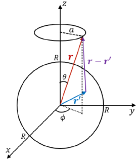
Figure 1: (Color online) The setting for detecting the current caused by the gravitational drag induced by the rotating body. The coordinates $\bf{r}$ is the observational point, and $\bf{r}^{\prime}$ is a point in the sphere to be integrated.

By using the multipole expansion, this is calculated as LL1 ; Ramos

$${\bf{A}}_{g}=-\frac{2G}{c^{3}r^{2}}{\bf{M}}\times{\bf{n}}$$ (2)

where ${\bf{n}}$ represents a unit vector direction of ${\bf{r}}$ and ${\bf{M}}$ is angular momentum of rotating sphere. The vector potential ${\bf{A}}_{g}$ is alternatively written in term of angle $\theta$ and $\phi$, which are indicated in Fig. 1, as

$${\bf{A}}_{g}=\frac{4GM\omega R^{2}}{5c^{3}r^{2}}\left(\sin\theta\sin\phi~{}{\bf{e}}_{x}-\sin\theta\cos\phi~{}{\bf{e}}_{y}\right)$$ (3)

where ${\bf{e}}_{x}$ and ${\bf{e}}_{y}$ are the unit vectors direction of $x$ and $y$, respectively.

3. Fluctuating current: Let us consider a superconducting circular ring, which is placed above the rotating body such that the ring is coaxial to the sphere, and the radius is given by $a$ which is prescribed to be smaller than the radius of the sphere as shown in Fig. 1. We adopt an ideal limit; the thickness of the ring is neglected. That is, the radius $a$ is extremely larger than the cross section of the ring.

Our argument is based on the Landau–Ginzburg (LG) free energy, for the order parameter $\psi$, that is written as Schmid ; Imry ; Langer ; LL2

$$F_{g}=\int\left[\frac{1}{2m}\psi^{*}\left(-i\hbar\nabla-mc{\bf A}_{g}\right)^{2}\psi+V(\psi^{*},\psi)\right]d{\bm{x}}$$

and the corresponding partition function is given by the functional integral:

$$Z=\int\exp[-\beta F_{g}]\mathcal{D}[\psi,\psi^{*}]$$ (4)

We make the following remark: We are concerned with the fluctuation current in the vicinity just above the superconducting transition temperature. Hence, consideration of the Meissner effect is not relevant in contrast to DeWitt procedure Dewitt , so no current is induced as a reaction of the Meissner effect in the gravito-magnetic field. Thus the gravito-magnetic vector potential directly enters in the same form as the usual electromagnetic one. As is implied from the above prescription, the gravito-magnetic vector potential $A_{g}$ has only $\phi$ component in terms of polar coordinate, which relates to electromagnetic vector potential $A$ as follows:

$$A=-\frac{mc^{2}}{2e}A_{g}$$ (5)

In the circular geometry, we have $F_{g}=\int\psi^{*}\Lambda\psi d\phi$, where $\Lambda$ is given by

$$\Lambda=\frac{\hbar^{2}}{2ma^{2}}\left(-i\frac{d}{d\phi}+\frac{\Phi}{\phi_{0}}\right)^{2}+|\alpha|,$$ (6)

with the flux $\Phi=\int Aad\phi$, and the flux quantum $\phi_{0}=hc/2e$ ($h$ means the Planck constant). Here, we note that the flux $\Phi$ is multiplied by $N$ when the winding number of the ring is $N$ times that of a basic circular ring. Equation (6) is the linear LG theory, for which the potential term $V$ is $\alpha\psi^{*}\psi$ and the parameter $\alpha$ is regarded as the “mass”, which is assumed to take a form $\alpha=C(T-T_{c})$ ($C$ is some constant, and $T_{c}$ means the transition temperature) Schmid ; Imry ; LL2 . The quartic term is omitted since the fluctuation effect is very small near the transition temperature.

Let us expand the order parameter as $\psi(t)=\sum_{n}a_{n}(t)\psi_{n}$ with $n$ taking an integer value running from $-\infty$ to $+\infty$ . Here $\psi_{n}$ are the eigenfunctions for the eigenvalue equations: $\Lambda\psi_{n}=\lambda_{n}\psi_{n}$. The eigenvalues are calculated to be

$$\lambda_{n}=\frac{{\hbar}^{2}}{2ma^{2}}\left(n+\frac{\Phi}{\phi_{0}}\right)^{2}+|\alpha|$$ (7)

and the corresponding eigenfunctions become $\psi_{n}=\frac{1}{\sqrt{2\pi}}\exp\left[in\phi\right]$. The partition function is thus calculated by using the functional integral (4):

$$Z = \int\exp\left[-\beta\sum_{n}\lambda_{n}a_{n}^{*}a_{n}\right]\prod_{n}da_{n}^{*}da_{n}$$ (8)

$$= \prod_{n=-\infty}^{+\infty}\frac{2\pi}{\beta\lambda_{n}}$$

from which one obtains the free energy $F=-k_{B}T\log Z$ (up to some additional constant). This is calculated as

$$F = k_{B}T\sum_{n}\log\left[\left(n+\frac{\Phi}{\phi_{0}}\right)^{2}+|\gamma|\right]$$ (9)

$$= k_{B}T\log\left[\cosh(2\pi\sqrt{\gamma})-\cos\left(2\pi\frac{\Phi}{\phi_{0}}\right)\right]$$

Here we have used the formula math

$$\sum_{n=-\infty}^{+\infty}\frac{1}{\left(n+\frac{\Phi}{\phi_{0}}\right)^{2}+x^{2}}=\frac{\pi}{x}\frac{\sinh(2\pi x)}{\cosh(2\pi x)-\cos\left(2\pi\frac{\Phi}{\phi_{0}}\right)}$$ (10)

Hence we can derive the fluctuating current along the ring, which is obtained by the formula: $J=c\frac{\partial F}{\partial\Phi}$, i.e.,

$$J=\frac{2\pi ck_{B}T}{\phi_{0}}\frac{\sin\left(2\pi\frac{\Phi}{\phi_{0}}\right)}{\cosh(2\pi\sqrt{\gamma})-\cos\left(2\pi\frac{\Phi}{\phi_{0}}\right)}$$ (11)

and use is made of the notation

$$\gamma=\frac{2ma^{2}}{{\hbar}^{2}}\alpha$$ (12)

together with the flux:

$$\left|\Phi\right| = 2\pi a\times\frac{mc^{2}}{2e}\times\left|{\bm{A}}_{g}\right|$$ (13)

$$= \frac{4\pi m}{5ec}\times\frac{GMVRa}{r^{2}}$$

where $V$ represents the rotating velocity $V=R\omega$.

If we are concerned with the state that is very close to the transition temperature; $T=T_{C}$, $\gamma$ can be regarded as a small quantity by noting $\alpha=C(T-T_{C})$. Further $\Phi/\phi_{0}$ is quite a small quantity by taking account of the fact that $G$ and $m/e$ are small in absolute sense. In addition, the second order of $\Phi/\phi_{0}$ is negligibly small, because the second order is smaller than the first order by 20 orders of magnitude. Under this condition, the current may be approximated as

$$J\sim 2ck_{B}T\frac{\Phi}{{\phi}_{0}^{2}\gamma}$$ (14)

The fluctuating current can be detected by observing (real) magnetic field produced by the Ampére law, which directs along the $z$-axis through the center of the circle, and the magnitude is $B=\frac{J}{a}$.

4. Discussion : In order to examine the behavior of the current in the very vicinity of the critical temperature, we rewrite this by introducing the “coherence length”, $\xi=\frac{\hbar}{\sqrt{2m\left|\alpha\right|}}$ Schmid , which is sufficiently larger than the size of the ring $a$, namely,

$$J=\frac{8}{5}\frac{k_{B}T}{\hbar c}\frac{me}{\hbar c}\frac{GMVR}{r^{2}a}{\xi}^{2}(T)$$ (15)

Near $T=T_{C}$, it is known that $\xi^{2}(T)=\xi_{0}^{2}\left(\frac{T_{C}}{T-T_{C}}\right)$ Schmid ; Imry , where $\xi_{0}$ means the coherence length at zero temperature, (which may be chosen to be the order $10^{-5}~{}{\rm m}$). By noting this fact, the current expression (15) indicates that the current gets a huge enhancement near $T=T_{c}$. Let us examine the order estimate by assuming the freely chosen parameters; $T,M,V,R,r,a$ as

$$J\sim 10^{-20}{\xi}^{2}(T)\left(\frac{T}{10~{}{\rm{K}}}\right)\left(\frac{M}{10^{3}~{}{\rm{kg}}}\right)\left(\frac{V}{10^{4}~{}{\rm{m/s}}}\right)$$

$$\left(\frac{R}{2~{}{\rm{m}}}\right)\left(\frac{2~{}{\rm{m}}}{r}\right)^{2}\left(\frac{10^{-3}~{}{\rm{m}}}{a}\right)~{}[{\rm{A}}]$$ (16)

If we could control the temperature $T$ such that it is extremely close to the transition temperature, we expect $\xi^{2}(T)\sim 10^{-2}$, which leads to the current of the order $10^{-22}$. In addition to the critical behavior, the flux $\Phi$ is proportional to winding number $N$ of the ring, so the current $J$ is also amplified by $N$ times. If we could take $N\sim 10^{5}$, the resultant current would be $J\sim 10^{-22}\times 10^{5}=10^{-17}[A]$.

Thus the present result is quite different from the classic DeWitt’s oneDewitt : the latter does not incorporate any enhancement mechanism arising from the critical temperature and the winding number. The enhancement of the present model is consequence of the LG formalism which is concerned with the state near critical temperature. As such, the order estimate given above is still tiny, even if it is magnified.

Despite such a feature, the present approach may open a novel aspect of exploring a possible effect of gravitational drag, which is provided by a framework of the LG theory. The detectability of this effect will depend on experimental innovations in the future.

This article appeared in Progress of Theoretical and Experimental Physics, 2017, 12I101 DOI: 10.1093/ptep/ptx171.

References

- (1) L. D. Landau and E. M. Lifshitz, Classical Theory of Fields, Fourth Edition, (Course of Theoretical Physics, Vol. 2, Butterworth–Heinemann, 1980).
- (2) C. Mller, The Theory of Relativity, (Oxford University Press, 1952).
- (3) A. Zee, Phys. Rev. Lett. 55, 2379 (1985).
- (4) J. Ramos and B. Mashhoon, Phys. Rev. D 73, 084003 (2006);
- (5) B. Mashhoon, in Reference Frames and Gravitomagnetism, edited by J. F. Pascual–Sánchez, L. Floria, A. San Miguel, F. Vicente (World Scientific, Singapore, 2001).
- (6) I. Ciufolini, Nature 449, 41 (2007).
- (7) B. S. DeWitt, Phys. Rev. Lett. 16, 1092 (1966).
- (8) V. B. Braginsky, C. M. Caves and K. S. Thorne, Phys. Rev. D 15, 2047 (1977).
- (9) D. Greenberger, Ann. Phys. 47, 116 (1968); D. Greenberger and A. W. Overhauser, Rev. Mod. Phys. 51, 43 (1979).
- (10) R. Colella, A. W. Overhauser, and S. A. Werner, Phys. Rev. Lett. 34, 1472 (1975).
- (11) S. J. Minter, K. W. McNelly, and R. Y. Chiao, Physica E, 42, 234 (2010).
- (12) M. Tajmar, C. J. de Matos, Physica C 420, 56 (2005).
- (13) J. Anandan, Phys. Rev. Lett. 47, 463 (1981).
- (14) A. Schmid, Phys. Rev. 180, 527 (1969).
- (15) Y. Imry, Introduction to Mesoscopic physics, 2nd ed. (Oxford Univercity Press, 2002).
- (16) J. S. Langer, V. Ambegaokar Phys. Rev. 164, 498 (1967).
- (17) E. M. Lifshitz and L. P. Pitaevski, Statistical Physics; part 2, (Course of Theoretical Physics, vol. 9. Butterworth-Heinemann, 1986).
- (18) K. Ito, Encyclopedic Dictionary of Mathematics, 4th ed. (MIT Press, Cambridge, 1993).