mvn2vec: Preservation and Collaboration in Multi-View Network Embedding
Abstract
Multi-view networks are broadly present in real-world applications. In the meantime, network embedding has emerged as an effective representation learning approach for networked data. Therefore, we are motivated to study the problem of multi-view network embedding with a focus on the optimization objectives that are specific and important in embedding this type of network. In our practice of embedding real-world multi-view networks, we explicitly identify two such objectives, which we refer to as preservation and collaboration. The in-depth analysis of these two objectives is discussed throughout this paper. In addition, the mvn2vec algorithms are proposed to (i) study how varied extent of preservation and collaboration can impact embedding learning and (ii) explore the feasibility of achieving better embedding quality by modeling them simultaneously. With experiments on a series of synthetic datasets, a large-scale internal Snapchat dataset, and two public datasets, we confirm the validity and importance of preservation and collaboration as two objectives for multi-view network embedding. These experiments further demonstrate that better embedding can be obtained by simultaneously modeling the two objectives, while not over-complicating the model or requiring additional supervision. The code and the processed datasets are available at http://yushi2.web.engr.illinois.edu/.
Index Terms:
Multi-view networks, network embedding, graph mining, representation learning.1 Introduction
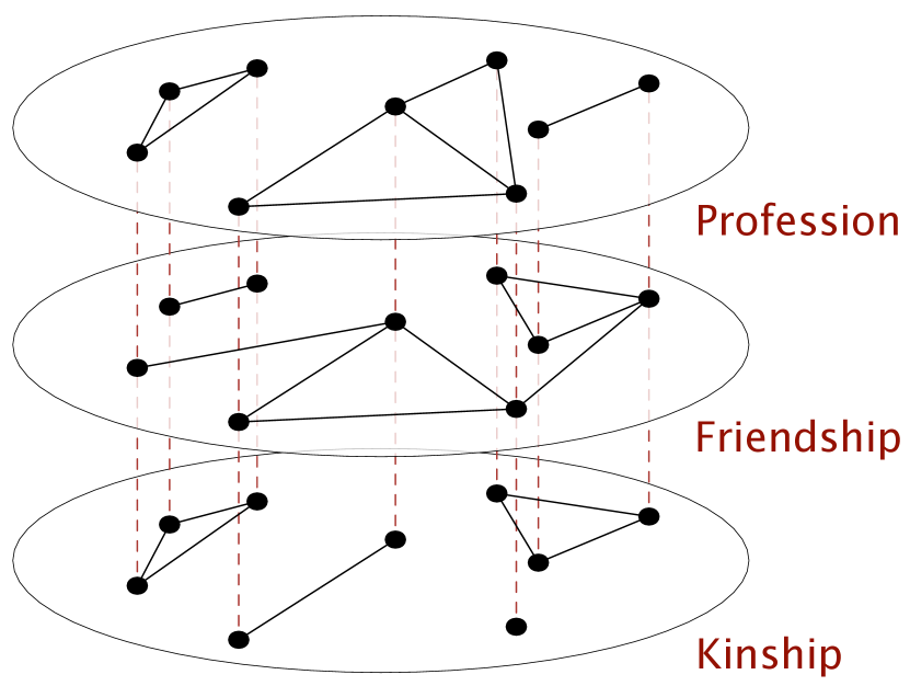
In real-world applications, objects can be associated with different types of relations. These objects and their relationships can be naturally represented by multi-view networks, i.e., multiplex networks or multi-view graphs [1, 2, 3, 4, 5, 6]. Figure 1(a) gives a toy multi-view network, where each view corresponds to a type of edge, and all views share the same set of nodes. As a more concrete example, a four-view network of users can be used to describe a social networking service with social relationship and interaction including friendship, following, message exchange, and post viewing. With the vast availability of multi-view networks, it is of interest to mine such networks.
In the meantime, network embedding has emerged as a scalable representation learning method for networked data [7, 8, 9, 10]. Specifically, network embedding projects nodes of networks into the embedding spaces. With the semantic information of each node encoded, the learned embedding can be directly used as features in various downstream applications [7, 8, 9]. Motivated by the success of network embedding for homogeneous networks [7, 8, 9, 10, 11, 12], where nodes and edges are untyped, we believe it is important to better understand multi-view network embedding.
To design embedding method for multi-view networks, the primary challenge lies in how to use the type information on edges from different views. As a result, we are interested in investigating the following two questions:
-
1.
With the availability of multiple edge types, what are the objectives that are specific and important to multi-view network embedding?
-
2.
Can we achieve better embedding quality by modeling these objectives jointly?
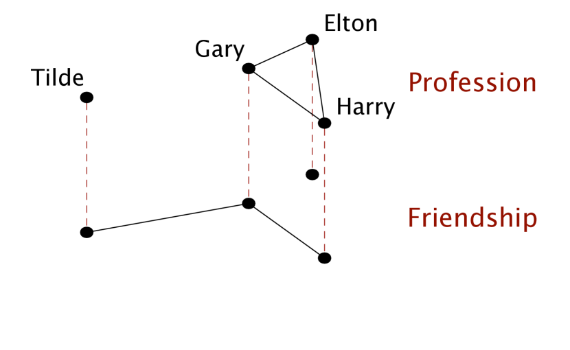
To answer the first question, we identify two such objectives, preservation and collaboration, from our practice of embedding real-world multi-view networks. Collaboration – In some datasets, edges between the same pair of nodes may be observed in different views due to shared latent reasons. For instance, in a social network, if we observe an edge between a user pair in either the message exchange view or the post viewing view, likely these two users are happy to be associated with each other. In such scenario, these views may complement each other, and embedding them jointly may potentially yield better results than embedding them independently. We call such synergetic effect in jointly embedding multiple views by collaboration, which is also the primary intuition behind most existing multi-view network algorithms [1, 2, 3, 4]. Preservation – On the other hand, it is possible for different network views to have different semantic meanings; it is also possible that a portion of nodes has completely disagreeing edges in different views since edges in different views are formed due to unrelated latent reasons. For example, the professional relationship may not always align well with friendship. If we embed the profession view and the friendship view in Figure 1(b) into the same embedding space, the embedding of Gary will be close to both Tilde and Elton. As a result, the embedding of Tilde will also not be too distant from Elton due to transitivity. However, this is not a desirable result, because Tilde and Elton are not closely related regarding either profession or friendship according to the original multi-view network. In other words, embedding in this way fails to preserve the unique information carried by different network views. We refer to such need for preserving unique information carried by different views as preservation. The detailed discussion of the validity and importance of preservation and collaboration is presented in Section 4.
Furthermore, the need for preservation and collaboration may co-exist in the same multi-view network. Two scenarios can result in this situation: (i) a pair of views are generated from very similar latent reason, while another pair of views carries completely different semantic meanings; and more subtly (ii) for the same pair of views, one portion of nodes has consistent edges in different views, while another portion of nodes have totally disagreeing edges in different views. One example of the latter scenario is that professional relationship does not align well with friendship in some cultures, whereas co-workers often become friends in certain other cultures [13]. Therefore, we are also interested in exploring the feasibility of achieving better embedding quality by modeling preservation and collaboration simultaneously, and we address this problem in Section 5 and beyond.
We note that, instead of proposing a sophisticated model that beats many baselines, this paper focus on the objectives of interests for multi-view network embedding. In experiments, we compare methods with a highlight on the roles the two objectives play in different scenarios. For the same reason, the scenarios where additional supervision is available are excluded from this paper, while the lessons learned from the unsupervised scenario can also be applied to the supervised multi-view network embedding algorithms. Additionally, node embedding learned by an unsupervised approach can directly apply to different downstream tasks, while supervised algorithms yield embedding specifically good for tasks where the supervision comes from. We summarize our contributions as follows.
-
1.
We study the objectives that are specific and important to multi-view network embedding and identify preservation and collaboration as two such objectives from the practice of embedding real-world multi-view networks.
-
2.
We explore the feasibility of attaining better embedding by simultaneously modeling preservation and collaboration, and propose two multi-view network embedding methods – mvn2vec-con and mvn2vec-reg.
-
3.
We conduct experiments with various downstream applications on four datasets. These experiments corroborate the validity and importance of preservation and collaboration and demonstrate the effectiveness of the proposed methods.
2 Related Work
Network embedding. Network embedding has emerged as an efficient and effective approach for learning distributed node representations. Instead of leveraging spectral properties of networks as commonly seen in traditional unsupervised feature learning approaches [14, 15, 16, 17], most network embedding methods are designed atop local properties of networks that involve links and proximity among nodes [7, 8, 9, 10, 11, 12, 18, 19]. Such methodology focusing on local properties has been shown to be more scalable. The designs of many recent network embedding algorithms are based on local properties of networks and can trace to the skip-gram model [20], which are shown to be scalable and widely applicable. To leverage the skip-gram model, various strategies have been proposed to define the context of a node in the network scenario [7, 8, 9, 11]. Beyond the skip-gram model, embedding methods for preserving certain other network properties can also be found in the literature [10, 21, 22, 23].
Multi-view networks. The majority of existing methods for multi-view networks aim to bring performance boost in traditional tasks, such as clustering [1, 2], classification [3], and dense subgraph mining [4]. Another line of research focuses on measuring and analyzing cross-view interrelations in multi-view networks [24, 25, 26, 6], but they do not discuss the objectives of embedding multi-view networks, nor do they study how their proposed measures and analyses can relate to the embedding learning of multi-view networks.
Multi-view network embedding. An attention-based collaboration framework is recently proposed for multi-view network embedding [27]. The problem setting of this work differs from ours since it requires supervision for its attention mechanism. Besides, this approach does not directly model preservation – one of the objectives that we deem important for multi-view network embedding. Since the final embedding derived via linear combination in this framework is a trade-off between representations from all views. A deep learning architecture has also been proposed for embedding multi-networks [28], where the multi-network is a more general concept than the multi-view network and allows many-to-many correspondence across networks. While the proposed model can be applied to the more specific multi-view networks, it does not focus on the study of the objectives of multi-view network embedding. Another group of related work studies the problem of jointly modeling multiple network views using latent space models [29, 30]. These works again do not model preservation. There exist a few more studies that touches the topic of multi-view network embedding[31, 32, 33, 34, 35] They do not model preservation and collaboration or do not aim to provide in-depth study of these objectives.
Besides, the problem of multi-view matrix factorization [36, 37, 38] is also related to multi-view network embedding. Liu et al. [38] propose a multi-view nonnegative matrix factorization model, which aims to minimize the distance between the adjacent matrix of each view and the consensus matrix. While these methods can generate a vector for each node; these vectors are modeled to suit certain tasks such as matrix completion or clustering, instead of to serve as distributed representations of nodes that can be used in different downstream applications.
Embedding techniques for other typed networks. In a bigger scope, a couple of studies have recently been conducted in embedding more general networks, such as heterogeneous information networks (HINs) [39, 40, 41, 42]. Some of them build the algorithms on top of meta-paths [41, 42], but meta-paths are usually more meaningful for HINs with multiple node types than multi-view networks. Some other methods are designed for networks with additional side information [40, 43] or particular structures [39, 44], which do not apply to multi-view networks. Most importantly, these methods are designed for networks they intend to embed, and therefore do not focus on the study of the particular needs and objectives for embedding multi-view networks.
Multi-relational network embedding or knowledge graph embedding embodies another direction of research that is relevant to multi-view network embedding [45, 46, 47, 48]. The study on this direction has a focus different and does not directly apply to our scenario because the relationships involved in these networks are often directed in nature. A popular family of such methods are translation based, where, in their language, the representation of a head entity is associated to that of a tail entity by that of a relation such that is assumed to be similar to [45, 46, 47, 48]. Such assumption is invalid for multi-view networks with undirected network views such as the friendship view in a social network.
3 Preliminaries
Definition 3.1 (Multi-View Network)
A multi-view network is a network consisting of a set of nodes and a set of views, where consists of all edges in view . If a multi-view network is weighted, then there exists a weight mapping such that is the weight of the edge , which joints nodes and in view .
Additionally, when context is clear, we use the network view of to denote the network .
Definition 3.2 (Network Embedding)
Network embedding aims at learning a (center) embedding for each node in a network, where is the dimension of the embedding space.
Besides the center embedding , a family of popular algorithms [20, 9] also deploy a context embedding for each node . Moreover, when the learned embedding is used as the feature vector for downstream applications, we take the center embedding of each node as feature following the common practice in algorithms involving context embedding.
| Symbol | Definition |
|---|---|
| The set of all network views | |
| The set of all nodes | |
| The set of all edges in view | |
| The list of random walk pairs from view | |
| The final embedding of node | |
| The center embedding of node w.r.t. view | |
| The context embedding of node w.r.t. view | |
| The hyperparameter on parameter sharing in mvn2vec-con | |
| The hyperparameter on regularization in mvn2vec-reg | |
| The dimension of the embedding space |
4 Preservation and Collaboration in Multi-View Network Embedding
In this section, we elaborate on the intuition and presence of preservation and collaboration – the two objectives introduced in Section 1. We first describe and investigate the motivating phenomena observed in our practice of embedding real-world multi-view networks, and then discuss how they can be explained by the two proposed objectives.
Two straightforward approaches for embedding multi-view networks. To extend untyped network embedding algorithms to multi-view networks, two straightforward yet practical approaches exist. We refer to these two approaches as the independent model and the one-space model. Specifically, we denote the embedding of node achieved by embedding only the view of the multi-view network, where is the dimension of the embedding space for network view . With such notation, the independent model and the one-space model are briefly introduced as follows, while further details can be found in Section 6.3.
-
•
The independent model. Embed each view independently, and then concatenate to derive the final embedding :
(1) where , and represents concatenation. In other words, the embedding of each node in the independent model resides in the direct sum of multiple embedding spaces. This approach preserves the information embodied in each view, but do not allow collaboration across different views in the embedding learning process.
-
•
The one-space model. Let the embedding for different views share parameters when learning the final embedding :
(2) Therefore, the final embedding space correlates with all network views. This approach allows different views to collaborate in learning a unified embedding, but do not preserve information specifically carried by each view. This property of the one-space model is corroborated by additional experiment in Section 6.5.
Further details on these models can be found in Section 6.3. It should also be noted that the embedding learned by the one-space model cannot be obtained by linearly combining in the independent model. This is because most network embedding models are non-linear.
| Dataset | Metric | independent | one-space |
|---|---|---|---|
| YouTube | ROC-AUC | 0.931 | 0.914 |
| PRC-AUC | 0.745 | 0.702 | |
| ROC-AUC | 0.724 | 0.737 | |
| PRC-AUC | 0.447 | 0.466 |
Embedding real-world multi-view networks by straightforward approaches. Two networks, YouTube and Twitter, are used in these exploratory experiments with users being nodes on each network. YouTube has three views representing common videos (cmn-vid), common subscribers (cmn-sub), and common friends (cmn-fnd) shared by each user pair, while Twitter has two views corresponding to replying (reply) and mentioning (mention) among users. The downstream evaluation task is to infer whether two users are friends, and the results are presented in Table II.
It can be seen that neither straightforward approach is categorically better than the other. In particular, the independent model consistently outperformed the one-space model in the YouTube experiment, while the one-space model outperformed the independent model in Twitter. Furthermore, we interpret the varying performance of the two approaches by the varying extent of needs for modeling preservation and modeling collaboration when embedding different networks. Specifically, recall that the independent model only captures preservation, while one-space only captures collaboration. As a result, we speculate if a certain dataset craves for more preservation than collaboration, the independent model will outperform the one-space model. Otherwise, the one-space model will win.
To corroborate our interpretation of the results, we examine the involved datasets and look into the agreement between information carried by different network views. We achieve this by a Jaccard coefficient based measurement, where the Jaccard coefficient is a similarity measure with range , defined as for set and set . For a pair of network views, a node can be connected to a different set of neighbors in each of the two views. We calculate the Jaccard coefficient between these two sets of neighbors. In Figure 2, we apply this measurement on both datasets and illustrate the proportion of nodes with the Jaccard coefficient greater than for each view pair.
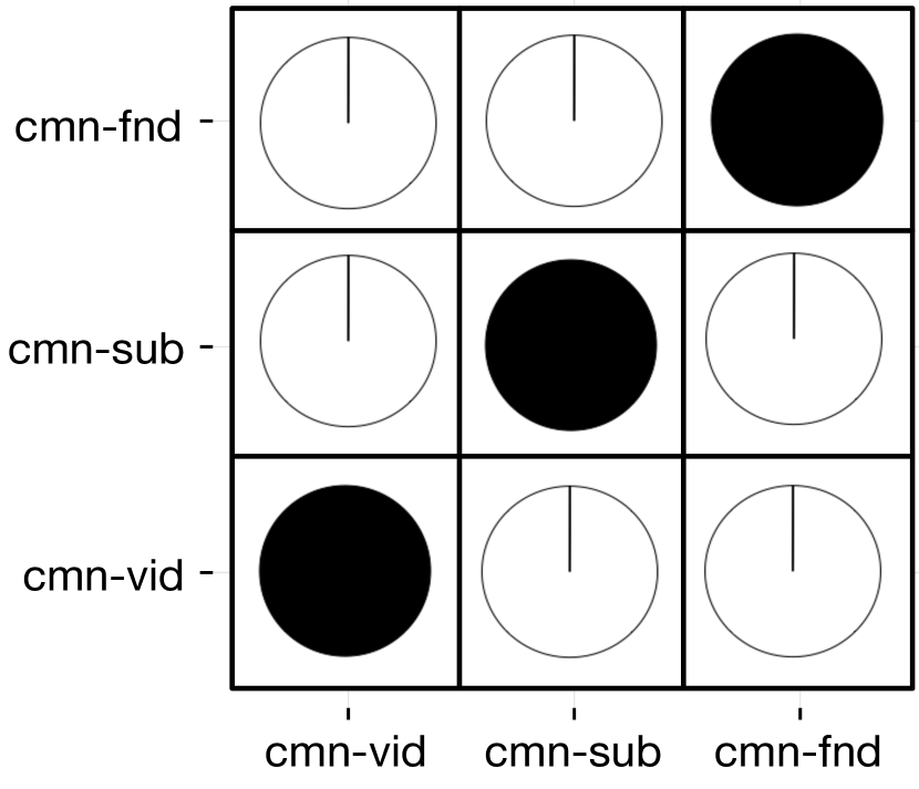
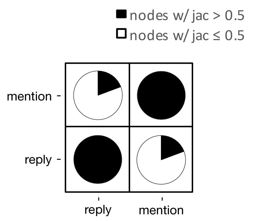
As presented in Figure 2, little agreement exists between each pair of different views on YouTube. As a result, it is not surprising that collaboration among different views is not as needed as preservation. On the other hand, a substantial portion of nodes has Jaccard coefficient greater than over different views on Twitter – not surprising to see modeling collaboration brings about more benefits than modeling preservation.
5 The mvn2vec Models
In the previous section, preservation and collaboration are identified as important objectives for multi-view network embedding. In the extreme cases, where only preservation is needed – each view carries a distinct semantic meaning – or only collaboration is needed – all views carry the same semantic meaning – simply choosing between independent and one-space may be enough to generate satisfactory results. However, it is of more interest to study the scenario where both preservation and collaboration co-exist in a multi-view network. Therefore, we are motivated to (i) study how varied extent of preservation and collaboration can impact embedding learning and (ii) explore the feasibility of achieving better embedding by simultaneously modeling both objectives. To this end, we propose two methods that capture both objectives, while not over-complicating the model or requiring additional supervision. These two approaches are named mvn2vec-con and mvn2vec-reg, where mvn2vec is short for multi-view network to vector, while con and reg stand for constrained and regularized.
As with the notation convention in Section 4, we denote and the center and context embedding, respectively, of node for view . Further given the network view , i.e., , we use an intra-view loss function to measure how well the current embedding can represent the original network view
| (3) |
We defer the detailed definition of this loss function to a later point of this section. We let for all out of convenience for model design. To further incorporate multiple views with the intention to model both preservation and collaboration, two approaches are proposed as follows.
mvn2vec-con. The mvn2vec-con model does not enforce further design on the center embedding in the hope of preserving the semantics of each individual view. To reflect collaboration, mvn2vec-con enforce constraints on the context embedding for parameter sharing across different views, so they are required to have the form
| (4) |
where and is a hyperparameter controlling the extend to which model parameters are shared. The greater the value of , the more the model enforces parameter sharing and thereby encouraging more collaboration across different views. The mvn2vec-con model solves the following optimization problem
| (5) |
After model learning, the final embedding for node is given by . We note that in the extreme case when is set to be , the model will be identical to the independent model in Section 4. To further distinguish the importance of different views, one can replace in Eq. (4) with a view-specific parameter , we defer the study of which to future work.
mvn2vec-reg. Instead of setting hard constraints on how parameters are shared across different views, the mvn2vec-reg model regularizes the embedding across different views and solves the following optimization problem
| (6) |
where is a hyperparameter, , , and is the - norm. This model captures preservation again by letting and to reside in the embedding subspace specific to view , while each of these subspaces are distorted via cross-view regularization to model collaboration. Similar to the mvn2vec-con model, the greater the value of the hyperparameter , the more the collaboration is encouraged, and the model is identical to the independent model when . To distinguish the importance of different views, one can replace in the formulation of with , and revise similarly. We also defer this study to future work for simplicity.
Intra-view loss function. There are many possible approaches to formulate the intra-view loss function in Eq. (3). In our framework, we adopt the random walk plus skip-gram approach, which is one of the most common in the literature [7, 8, 11]. Specifically, for each view , multiple rounds of random walks are sampled starting from each node in . In any random walk, a node and a neighboring node constitute one random walk pair, and a list of random walk pairs can thereby be derived. We will describe the detailed description of the generation of later in this section. The intra-view function is then given by
| (7) |
where .
Model inference. To optimize the objectives in Eq. (5) and (6), we opt to asynchronous stochastic gradient descent (ASGD) [49] following existing skip-gram–based algorithms [7, 8, 11, 9, 20]. In this regard, from all views are joined and shuffled to form a new list of random walk pairs for all views. Then each step of ASGD draws one random walk pair from and updates corresponding model parameters with one-step gradient descent. Negative sampling is adopted as in other skip-gram–based methods [7, 8, 11, 9, 20], which approximates in Eq. (7) by where is the sigmoid function, is the negative sampling rate, is the noise distribution, and is the number of occurrences of node in [20].
With negative sampling, the objective function involving one walk pair from view in mvn2vec-con is
On the other hand, the objective function involving from view in mvn2vec-reg is
The gradients of the above two objective function used for ASGD are provided as follows.
mvn2vec-con :
| (8) | ||||
| (9) |
| (10) |
mvn2vec-reg :
| (11) | ||||
| (12) |
| (13) |
Note that in implementation, should be the number of views in which is associated with at least one edge.
Random walk pair generation. Without additional supervision, we assume the equal importance of different network views and sample the same number of random walks from each view. To determine , we denote the number of nodes that are not isolated from the rest of the network in view , , and let , where is a hyperparameter to be specified. Given a network view , we generate random walk pairs following existing studies [8, 7, 11], where the transition probabilities from a node are proportional to the weights of all its outgoing edges. Specifically, each random walk is of length , and or random walks are sampled from each non-isolated node in view , yielding a total of random walks. For each node in any random walk, this node and any other node within a window of size form a random walk pair that is then added to .
Complexity analysis. For every view, random walks are generated independently by existing method [8, 7, 11]. An analysis similar to that in related work [7] can show the overall complexity is , which is linear to the number of views . For model inference, the number of ASGD steps is , linear to , , and . Each ASGD step computes gradients provided in Eq. (8)–(13), which is again linear to . Therefore, the overall complexity of model inference is quadratic to the number of views .
We summarize both the mvn2vec-con algorithm and the mvn2vec-reg algorithm in Algorithm 1.
6 Experiments
In this section, we further corroborate the intuition of preservation and collaboration, and demonstrate the feasibility of simultaneously model these two objectives. We first perform a case study on a series of synthetic multi-view networks that have varied extent of preservation and collaboration. Next, we introduce the real-world datasets, baselines, and experiment setting for more comprehensive quantitative evaluations. Lastly, we analyze the evaluation results and provide further discussion.
6.1 Case Study – Varied preservation and collaboration on Synthetic Data
To directly study the relative performance of different models on networks with varied extent of preservation and collaboration, we design a series of synthetic networks and conduct a multi-class classification task.
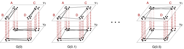
We denote each of these synthetic networks by , where is referred to as the intrusion probability. Each has nodes and views – and . Furthermore, each node is associated to one of the class labels – A, B, C, or D – and each class has exactly nodes. Before introducing the more general , we first describe the process for generating as follows:
-
1.
generate one random network over all nodes with label A or B, and another over all nodes with label C or D; put all edges in these two random networks into view ;
-
2.
generate one random network over all nodes with label A or C, and another over all nodes with label B or D; put all edges in these two random networks into view .
To generate each of the four aforementioned random networks, we adopt the widely used preferential attachment process with one edge to attach from a new node to existing nodes, where the preferential attachment process is a widely used method for generating networks with power-law degree distribution. With this design, view carries the information that nodes labeled A or B should be treated differently from nodes labeled C or D, while reflects that nodes labeled A or C are different from nodes labeled B or D. More generally, are generated with the following tweak from : when putting an edge into one of the two views, with probability , the edge is put into the other view instead of the view specified in the generation process.
It is worth noting that greater favors more collaboration, while smaller favors more preservation. In the extreme case where , only collaboration is needed in the network embedding process. This is because every edge has equal probability to fall into view or view of , and there is hence no information carried specifically by either view that should be preserved.
For each , independent, one-space, mvn2vec-con, and mvn2vec-reg are tested. Atop the embedding learned by each model, we apply logistic regression with cross-entropy to carry out the multi-class evaluation tasks. Parameters are tuned on a validation dataset sampled from the class labels. Classification accuracy and cross-entropy on a different test dataset are reported in Figure 4.
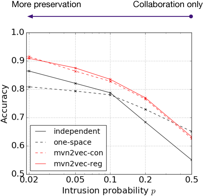
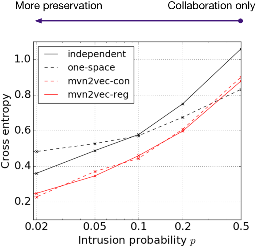
Observations. From Figure 4, we make three observations. (i) independent performs better than one-space in case is small – when preservation is the dominating objective in the network – and one-space performs better than independent in case is large – when collaboration is dominating. (ii) The two proposed mvn2vec models perform better than both independent and one-space except when is close to , which implies it is indeed possible for mvn2vec to achieve better performance by simultaneously modeling preservation and collaboration. (iii) When is close to , one-space performs the best. This is expected because no preservation is needed in , and any attempts to additionally model preservation shall not boost, if not impair, the performance.
6.2 Data Description and Evaluation Tasks
We perform further quantitative evaluations on three real-world multi-view networks: Snapchat, YouTube, and Twitter. The key statistics are summarized in Table III, and we describe these datasets as follows.
YouTube. YouTube is a video-sharing website. We use the YouTube dataset made publicly available by the Social Computing Data Repository [50]111http://socialcomputing.asu.edu/datasets/YouTube. From this dataset, a network with three views is constructed, where each node is a core user, and the edges in the three views represent the number of common friends, the number of common subscribers, and the number of common favorite videos, respectively. Note that the core users are those from which the author of the dataset crawled the data, and their friends can fall out of the scope of the set of core users. Without user label available for classification, we perform only link prediction task on top of the user embedding. This task aims at inferring whether two core users are friends, which has also been used for evaluation by existing research [27]. Each core user forms positive pairs with his or her core friends, and we randomly select times as many non-friend core users to form negative examples. Records are split into training, validation, and test sets as in the link prediction task on YouTube.
Twitter. Twitter is an online news and social networking service. We use the Twitter dataset made publicly available by the Social Computing Data Repository [51]222https://snap.stanford.edu/data/higgs-twitter.html. From this dataset, a network with two views is constructed, where each node is a user, and the edges in the two views represent the number of replies and the number of mentions, respectively. Again, we evaluate using a link prediction task that infers whether two users are friends as in existing research [27]. Negative examples generation and training–validation–test split method are the same as in the YouTube dataset.
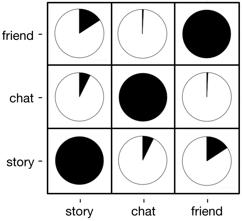
Snapchat. Snapchat is a multimedia social networking service. On the Snapchat multi-view social network, each node is a user, and the three views correspond to friendship, chatting, and story viewing333https://support.snapchat.com/en-US/a/view-stories. We perform experiments on the sub-network consisting of all users from Los Angeles. The data used to construct the network are collected from two consecutive weeks in the Spring of 2017. Additional data for downstream evaluation tasks are collected from the following week (week 3). We perform a multi-label classification task, and a link prediction task on top of the same user embedding learned from each network. For classification, we classify whether or not a user views each of the most popular discover channels444https://support.snapchat.com/en-US/a/discover-how-to according to the user viewing history in week 3, which aims at inferring users’ preference and thereby guide product design in content serving. For each channel, the users who view this channel are labeled positive, and we randomly select times as many users who do not view this channel as negative examples. These records are then randomly split into training, validation, and test sets. This is a multi-label classification problem that aims at inferring users’ preference on different discover channels and can therefore guide product design in content serving. For link prediction, we predict whether two users would view the stories posted by each other in week 3, which aims to estimate the likelihood of story viewing between friends, so as to re-rank stories accordingly. Negative examples are the users who are friends but do not have story viewing in the same week. It is worth noting that this definition yields more positive examples than negative examples, which is the cause of a relatively high AUPRC score observed in experiments. These records are then randomly split into training, validation, and test sets with the constraint that a user appears as the viewer of a record in at most one of the three sets. This task aims to estimate the likelihood of story viewing between friends so that the application can rank stories accordingly.
We also provide the Jaccard coefficient based measurement on Snapchat in Figure 5. It can be seen that the cross-view agreement between each pair of views in the Snapchat network falls in between YouTube and Twitter as presented previously in Section 2.
For each evaluation task on all three networks, training, validation, and test sets are derived in a shuffle split manner with an –– ratio. We split the data and repeat the experiments times to compute the mean and its standard error under each metric. Furthermore, a node is excluded from evaluation if it is isolated from other nodes in at least one of the multiple views. This processing ensures every node has a valid representation when embedding only one network view.
| Dataset | # views | # nodes | # edges |
|---|---|---|---|
| Snapchat | 3 | 7,406,859 | 131,729,903 |
| YouTube | 3 | 14,900 | 7,977,881 |
| 2 | 116,408 | 183,341 |
6.3 Baselines and Experimental Setup
In this section, we describe the baselines as well as experimental setup for both embedding learning and downstream evaluation tasks.
Baselines. Quantitative evaluation results are obtained by applying downstream learner upon embedding learned by a given embedding method. Therefore, for fair comparisons, we use the same downstream learner in the same evaluation task. We experiment with both in-house baselines and external baselines from related work. Since our study aims at understanding the objectives of multi-view network embedding, we build the following in-house embedding methods from the same random work plus skip-gram approach with the same model inference method as described in Section 5. Independent – As introduced in Section 4, the independent model is equivalent to mvn2vec-con when , and to mvn2vec-reg when . It preserves the information embodied in each view, but do not allow collaboration across different views in the embedding process. One-space – Also introduced in Section 4, the one-space enables different views to collaborate in learning a unified embedding, but do not preserve information specifically carried by each view. View-merging – The view-merging model first merges all network views into one unified view, and then learn the embedding of this single unified view. To comply with the assumed equal importance of all network views, we rescale the weights of edges proportionally in each view to the same total weight. This method serves as an alternate approach to one-space in modeling collaboration. The difference between view-merging and one-space essentially lies in whether or not random walks can cross different views. We note that just like one-space, view-merging does not model preservation. Single-view – For each network view, the single-view model learns embedding from only one view as a sanity check to verify whether introducing more than one view does bring in informative signals in each evaluation task. In other words, it is identical to embedding only one of the multiple network views using the DeepWalk algorithm [8], or equivalently node2vec with both return parameter and in-out parameter set to [7]. This baseline is used to as a sanity check to verify whether introducing more than one view does bring in informative signals in each evaluation task.
We also experiment with two external baselines that have executable implementation released by the original authors and can be applied to our experiment setting with minimal tweaks. Note that the primary observations and conclusions made in the experiments would still hold without comparing to these external baselines. MVE [27] – An attention-based semi-supervised method for multi-view network embedding. The released implementation supports supervision from classification tasks. For fair comparison, in our unsupervised link prediction experiments, we assign the same dummy class label to randomly selected nodes. We have observed that the percentage of nodes receiving such dummy supervision does not significantly affect the evaluation results in additional experiments. DMNE [28] – A deep learning architecture for multi-network embedding, where the multi-network is a more general concept than the multi-view network. As a more complex model, the released DMNE implementation takes significantly more time to train on our datasets, and we hence use only the default hyperparameters. The authors commented in the original paper that this implementation can be further sped up with additional parallelization. We experiment with two external baselines on the smaller YouTube and Twitter dataset for scalability reason.
Downstream learners. For fair comparisons, we apply the same downstream learner onto the features derived from each embedding method. Specifically, we use the scikit-learn555http://scikit-learn.org/stable/ implementation of logistic regression with -2 regularization and the SAG solver for both classification and link prediction tasks. Regularization coefficient in the logistic regression is always tuned to the best on the validation set. Following existing research [9], each embedding vector is post-processed by projecting onto the unit -2 sphere. In multi-label classification tasks, the feature is simply the embedding of each node, and an independent logistic regression model is trained for for each label. In link prediction tasks, features of node pairs are derived by the Hadamard product of the embedding vectors of the two involved node as suggested by previous work [7].
Hyperparameters. For independent, mvn2vec-con, and mvn2vec-reg, we set embedding space dimension . For single-view, we set . For all other methods, we experiment with both and , and report the better result. To generate random walk pairs, we set and . For Snapchat, we set due to its large scale and set for all other datasets. The negative sampling rate is set to be for all models, and each model is trained for epoch. In Figure 4, Table IV, Table V, and Figure 6, and in the mvn2vec models are also tuned on the validation dataset. The impact of and on model performance is further discussed in Section 6.5.
Metrics. For link prediction tasks, we use two widely used metrics: the area under the receiver operating characteristic curve (ROC-AUC) and the area under the precision-recall curve (PRC-AUC). The receiver operating characteristic curve (ROC) is derived from plotting true positive rate against false positive rate as the threshold varies, and the precision-recall curve (PRC) is created by plotting precision against recall as the threshold varies. Higher values are preferable for both metrics. For multi-label classification tasks, we also compute the ROC-AUC and the PRC-AUC for each label and report the mean value averaged across all labels.
| Dataset | YouTube | |||
|---|---|---|---|---|
| Metric | ROC-AUC | PRC-AUC | ROC-AUC | PRC-AUC |
| worst single-view | 0.831 (0.002) | 0.515 (0.004) | 0.597 (0.001) | 0.296 (0.001) |
| best single-view | 0.904 (0.002) | 0.678 (0.004) | 0.715 (0.001) | 0.428 (0.001) |
| independent | 0.931 (0.001) | 0.745 (0.003) | 0.724(0.001) | 0.447 (0.001) |
| one-space | 0.914 (0.001) | 0.702 (0.004) | 0.737 (0.001) | 0.466 (0.001) |
| view-merging | 0.912 (0.001) | 0.699 (0.004) | 0.741 (0.001) | 0.469 (0.001) |
| MVE [27] | 0.918 (0.001) | 0.714 (0.001) | 0.727 (0.001) | 0.451 (0.001) |
| DMNE [28] | 0.749 (0.001) | 0.311 (0.001) | — | — |
| mvn2vec-con | 0.932 (0.001) | 0.746 (0.001) | 0.727 (0.000) | 0.453 (0.001) |
| mvn2vec-reg | 0.934 (0.001) | 0.754 (0.003) | 0.754 (0.001) | 0.478 (0.001) |
| Dataset | Snapchat | |||
|---|---|---|---|---|
| Task | Link prediction | Classification | ||
| Metric | ROC-AUC | PRC-AUC | ROC-AUC | PRC-AUC |
| worst single-view | 0.587 (0.001) | 0.675 (0.001) | 0.634 (0.001) | 0.252 (0.001) |
| best single-view | 0.592 (0.001) | 0.677 (0.002) | 0.667 (0.002) | 0.274 (0.002) |
| independent | 0.617 (0.001) | 0.700 (0.001) | 0.687 (0.001) | 0.293 (0.002) |
| one-space | 0.603 (0.001) | 0.688 (0.002) | 0.675 (0.001) | 0.278 (0.001) |
| view-merging | 0.611 (0.001) | 0.693 (0.002) | 0.672 (0.001) | 0.279 (0.001) |
| mvn2vec-con | 0.626 (0.001) | 0.709 (0.001) | 0.693 (0.001) | 0.298 (0.001) |
| mvn2vec-reg | 0.638 (0.001) | 0.712 (0.002) | 0.690 (0.001) | 0.296 (0.002) |
6.4 Quantitative Evaluation Results on Real-World Datasets
The main quantitative evaluation results are presented in Table IV and Table V. Among the in-house baselines and the proposed mvn2vec models, all models leveraging multiple views outperformed those using only one view, which justifies the necessity of using multi-view networks. Moreover, one-space and view-merging had comparable performance on each dataset. This is an expected outcome because they both only model collaboration and differ from each other merely in whether random walks are performed across network views.
In case the need for either collaboration or preservation prevails. On YouTube, the proposed mvn2vec models perform as good but do not significantly exceed the baseline independent model. Recall that the need for preservation in the YouTube network is overwhelmingly dominating as discussed in Section 4. As a result, it is not surprising to see that additionally modeling collaboration does not bring about significant performance boost in such extreme case. On Twitter, collaboration plays a more important role than preservation, as confirmed by the better performance of one-space than independent. Furthermore, mvn2vec-reg achieved better performance than all baselines, while mvn2vec-con outperformed independent by further modeling collaboration, but failed to exceed one-space. This phenomenon can be explained by the fact that in mvn2vec-con are set to be independent regardless of its hyperparameter , and mvn2vec-con’s capability of modeling collaboration is bounded by this design.
In case both collaboration and preservation are indispensable. The Snapchat network used in our experiments lies in between YouTube and Twitter in terms of the need for preservation and collaboration. The proposed two mvn2vec models both outperformed all baselines under all metrics. In other words, this experiment result shows the feasibility of gaining performance boost by simultaneously model preservation and collaboration without over-complicating the model or adding supervision.
The multi-label classification results on Snapchat are presented in Table V. As with the previous link prediction results, the two mvn2vec model both outperformed all baselines under all metrics, with a difference that mvn2vec-con performed better in this classification task, while mvn2vec-reg outperformed better in the previous link prediction task. Overall, while mvn2vec-con and mvn2vec-reg may have different advantages in different tasks, they both outperformed all baselines by simultaneously modeling preservation and collaboration on the Snapchat network, where both preservation and collaboration co-exist.
External baeslines. MVE underperformed mvn2vec models on YouTube. We interpret this outcome as MVE is a collaboration framework that does not explicitly model preservation, which has been shown to be needed in the YouTube datasets. Meanwhile, MVE did not get performance boost from its attention mechanism since the experiment setting forbids it from consuming informative supervision as discussed in Section 6.3. Without additional optimization, the released DMNE implementation did not finish training on the Twitter dataset after two days on a machine with 40 cores of Intel(R) Xeon(R) CPU E5-2680 v2 @ 2.80GHz. The comparatively worse performance of DMNE on YouTube should partially attribute to the use of default hyperparameters as described in Section 6.3. Another possible explanation is that DMNE is designed for the more general multi-networks, not optimized for multi-view networks.
These observations in combine demonstrated the feasibility of gaining performance boost by simultaneously modeling preservation and collaboration without over-complicating the model or requiring additional supervision.
6.5 Hyperparameter Study
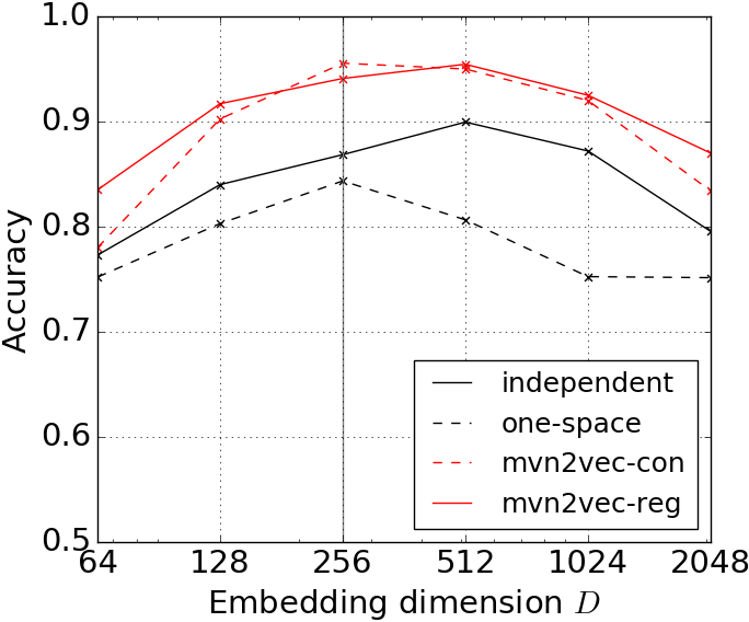
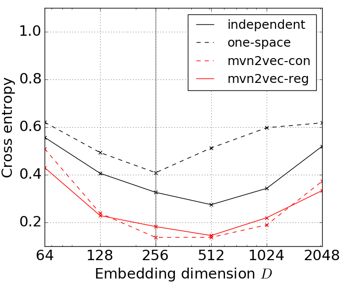
Impact of embedding dimension. To rule out the possibility that one-space could actually preserve the view-specific information as long as the embedding dimension were set to be large enough, we study the impact of embedding dimension. Particularly, we carry out the multi-class classification task on under varied embedding dimensions. Note that is used in this experiment because it has the need for modeling preservation as discussed in Section 6.1. As presented in Figure 6, one-space achieves its best performance at , which is worse than independent at , let alone the best performance of independent at . Therefore, one cannot expect one-space to preserve the information carried by different views by employing embedding space with large enough dimension.
Besides, all four models achieve their best performance with around 256512. Particularly, one-space uses the smallest embedding dimension to reach peak performance. This is expected since one-space does not divide the embedding space to suit multiple views and have more freedom in exploiting an embedding space with given dimension.
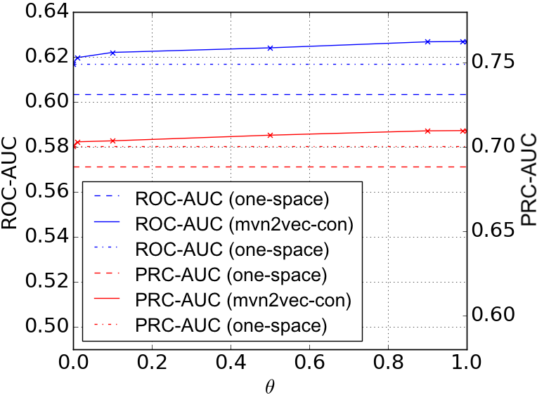
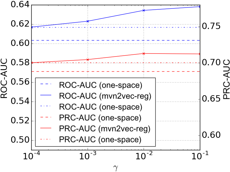
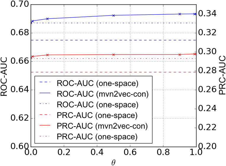
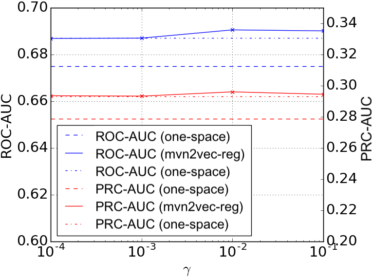
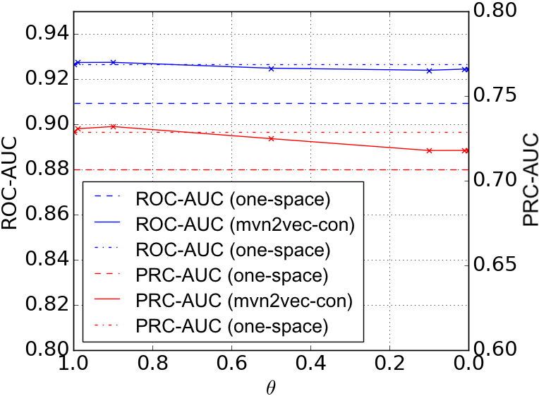
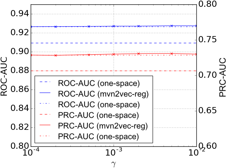
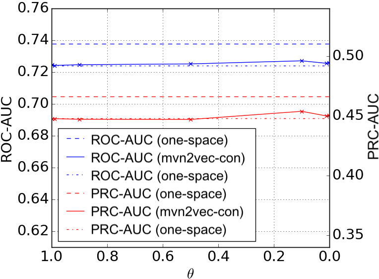
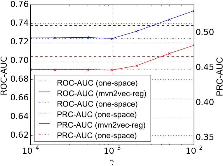
Impact of for mvn2vec-con and for mvn2vec-reg. We also study the impact of for mvn2vec-con and for mvn2vec-reg, which corroborated the observations in Section 6.4. With results presented in Figure 7, we first focus on the Snapchat network. Starting from , where only preservation was modeled, mvn2vec-reg performed progressively better as more collaboration kicked in by increasing . The peak performance was reached between and . On the other hand, the performance of mvn2vec-con improved as grew. Recall that even in case , mvn2vec-con still have independent in each view. This prevented mvn2vec-con from promoting more collaboration.
On YouTube, the mvn2vec models did not significantly outperform independent no matter how and varied due to the dominant need for preservation as discussed in Section 4 and 6.4.
On Twitter, mvn2vec-reg outperformed one-space when was large, while mvn2vec-con could not beat one-space for reasons discussed in Section 6.4. This also echoed mvn2vec-con’s performance on Snapchat as discussed in the first paragraph of this section.
7 Conclusion and Future Work
We identified and studied the objectives that are specific and important to multi-view network embedding, i.e. preservation and collaboration. We then explored the feasibility of better embedding by simultaneously modeling both objectives, and proposed two multi-view network embedding methods. Experiments with various downstream tasks were conducted on a series of synthetic networks and three real-world multi-view networks from distinct sources, including two public datasets and a large-scale internal Snapchat dataset. The results corroborated the validity and importance of preservation and collaboration as two optimization objectives, and demonstrated the effectiveness of the proposed mvn2vec methods.
Knowing the existence of the identified objectives, future works include modeling different extent of preservation and collaboration for different pairs of views in multi-view embedding. It is also rewarding to explore supervised methods for task-specific multi-view network embedding that jointly model preservation and collaboration.
Acknowledgments. This work was sponsored in part by U.S. Army Research Lab. under Cooperative Agreement No. W911NF-09-2-0053 (NSCTA), DARPA under Agreement No. W911NF-17-C-0099, National Science Foundation IIS 16-18481, IIS 17-04532, and IIS-17-41317, DTRA HDTRA11810026, and grant 1U54GM114838 awarded by NIGMS through funds provided by the trans-NIH Big Data to Knowledge (BD2K) initiative (www.bd2k.nih.gov). Any opinions, findings, and conclusions or recommendations expressed in this document are those of the author(s) and should not be interpreted as the views of any U.S. Government. The U.S. Government is authorized to reproduce and distribute reprints for Government purposes notwithstanding any copyright notation hereon.
References
- [1] A. Kumar, P. Rai, and H. Daume, “Co-regularized multi-view spectral clustering,” in NIPS, 2011, pp. 1413–1421.
- [2] D. Zhou and C. J. Burges, “Spectral clustering and transductive learning with multiple views,” in ICML, 2007.
- [3] V. Sindhwani and P. Niyogi, “A co-regularized approach to semi-supervised learning with multiple views,” in ICML Workshop on Learning with Multiple Views, 2005.
- [4] J. Pei, D. Jiang, and A. Zhang, “On mining cross-graph quasi-cliques,” in KDD. ACM, 2005, pp. 228–238.
- [5] O. Frank and K. Nowicki, “Exploratory statistical analysis of networks,” Annals of Discrete Mathematics, vol. 55, 1993.
- [6] P. Pattison and S. Wasserman, “Logit models and logistic regressions for social networks: II. multivariate relations,” BJMSP, vol. 52, no. 2, pp. 169–194, 1999.
- [7] A. Grover and J. Leskovec, “node2vec: Scalable feature learning for networks,” in KDD, 2016.
- [8] B. Perozzi, R. Al-Rfou, and S. Skiena, “Deepwalk: Online learning of social representations,” in KDD, 2014.
- [9] J. Tang, M. Qu, M. Wang, M. Zhang, J. Yan, and Q. Mei, “Line: Large-scale information network embedding,” in WWW, 2015.
- [10] D. Wang, P. Cui, and W. Zhu, “Structural deep network embedding,” in KDD, 2016.
- [11] B. Perozzi, V. Kulkarni, H. Chen, and S. Skiena, “Don’t walk, skip! online learning of multi-scale network embeddings,” in ASONAM, 2017.
- [12] M. Ou, P. Cui, J. Pei, Z. Zhang, and W. Zhu, “Asymmetric transitivity preserving graph embedding.” in KDD, 2016.
- [13] J. P. Alston, “Wa, guanxi, and inhwa: Managerial principles in japan, china, and korea,” Business Horizons, vol. 32, no. 2, 1989.
- [14] M. Belkin and P. Niyogi, “Laplacian eigenmaps and spectral techniques for embedding and clustering,” in NIPS, vol. 14, no. 14, 2001, pp. 585–591.
- [15] S. T. Roweis and L. K. Saul, “Nonlinear dimensionality reduction by locally linear embedding,” Science, vol. 290, no. 5500, pp. 2323–2326, 2000.
- [16] J. B. Tenenbaum, V. De Silva, and J. C. Langford, “A global geometric framework for nonlinear dimensionality reduction,” Science, 2000.
- [17] S. Yan, D. Xu, B. Zhang, H.-J. Zhang, Q. Yang, and S. Lin, “Graph embedding and extensions: A general framework for dimensionality reduction,” PAMI, 2007.
- [18] M. Zhang and Y. Chen, “Weisfeiler-lehman neural machine for link prediction,” in KDD, 2017, pp. 575–583.
- [19] L. F. Ribeiro, P. H. Saverese, and D. R. Figueiredo, “struc2vec: Learning node representations from structural identity,” in KDD, 2017.
- [20] T. Mikolov, I. Sutskever, K. Chen, G. S. Corrado, and J. Dean, “Distributed representations of words and phrases and their compositionality,” in NIPS, 2013.
- [21] M. Niepert, M. Ahmed, and K. Kutzkov, “Learning convolutional neural networks for graphs,” in ICML, 2016.
- [22] P. Veličković, G. Cucurull, A. Casanova, A. Romero, P. Liò, and Y. Bengio, “Graph attention networks,” in ICLR, 2018.
- [23] T. N. Kipf and M. Welling, “Semi-supervised classification with graph convolutional networks,” in ICLR, 2017.
- [24] F. Battiston, V. Nicosia, and V. Latora, “Structural measures for multiplex networks,” Physical Review E, 2014.
- [25] M. De Domenico, A. Solé-Ribalta, E. Cozzo, M. Kivelä, Y. Moreno, M. A. Porter, S. Gómez, and A. Arenas, “Mathematical formulation of multilayer networks,” Physical Review X, 2013.
- [26] M. Berlingerio, M. Coscia, F. Giannotti, A. Monreale, and D. Pedreschi, “Multidimensional networks: foundations of structural analysis,” World Wide Web, 2013.
- [27] M. Qu, J. Tang, J. Shang, X. Ren, M. Zhang, and J. Han, “An attention-based collaboration framework for multi-view network representation learning,” in CIKM, 2017.
- [28] J. Ni, S. Chang, X. Liu, W. Cheng, H. Chen, D. Xu, and X. Zhang, “Co-regularized deep multi-network embedding,” in WWW, 2018.
- [29] I. Gollini and T. B. Murphy, “Joint modelling of multiple network views,” JCGS, 2014.
- [30] D. Greene and P. Cunningham, “Producing a unified graph representation from multiple social network views,” in Web Science Conference, 2013.
- [31] G. Ma, L. He, C.-T. Lu, W. Shao, P. S. Yu, A. D. Leow, and A. B. Ragin, “Multi-view clustering with graph embedding for connectome analysis,” in CIKM, 2017.
- [32] H. Zhang, L. Qiu, L. Yi, and Y. Song, “Scalable multiplex network embedding.” in IJCAI, 2018.
- [33] W. Liu, P.-Y. Chen, S. Yeung, T. Suzumura, and L. Chen, “Principled multilayer network embedding,” in ICDM Workshops, 2017.
- [34] N. Ning, B. Wu, and C. Peng, “Representation learning based on influence of node for multiplex network,” in DSC, 2018.
- [35] Y. Cen, X. Zou, J. Zhang, H. Yang, J. Zhou, and J. Tang, “Representation learning for attributed multiplex heterogeneous network,” in KDD, 2019.
- [36] D. Greene and P. Cunningham, “A matrix factorization approach for integrating multiple data views,” Machine Learning and Knowledge Discovery in Databases, pp. 423–438, 2009.
- [37] A. P. Singh and G. J. Gordon, “Relational learning via collective matrix factorization,” in Proceedings of the 14th ACM SIGKDD international conference on Knowledge discovery and data mining. ACM, 2008, pp. 650–658.
- [38] J. Liu, C. Wang, J. Gao, and J. Han, “Multi-view clustering via joint nonnegative matrix factorization,” in SDM, vol. 13. SIAM, 2013, pp. 252–260.
- [39] J. Tang, M. Qu, and Q. Mei, “Pte: Predictive text embedding through large-scale heterogeneous text networks,” in KDD. ACM, 2015.
- [40] S. Chang, W. Han, J. Tang, G.-J. Qi, C. C. Aggarwal, and T. S. Huang, “Heterogeneous network embedding via deep architectures,” in KDD, 2015.
- [41] T.-y. Fu, W.-C. Lee, and Z. Lei, “Hin2vec: Explore meta-paths in heterogeneous information networks for representation learning,” in CIKM, 2017.
- [42] Y. Dong, N. V. Chawla, and A. Swami, “metapath2vec: Scalable representation learning for heterogeneous networks,” in KDD, 2017.
- [43] H. Dai, B. Dai, and L. Song, “Discriminative embeddings of latent variable models for structured data,” in ICML, 2016.
- [44] H. Gui, J. Liu, F. Tao, M. Jiang, B. Norick, and J. Han, “Large-scale embedding learning in heterogeneous event data,” in ICDM, 2016.
- [45] X. Li, H. Hong, L. Liu, and W. K. Cheung, “A structural representation learning for multi-relational networks,” in IJCAI, 2017.
- [46] A. Bordes, N. Usunier, A. Garcia-Duran, J. Weston, and O. Yakhnenko, “Translating embeddings for modeling multi-relational data,” in NIPS, 2013.
- [47] Z. Wang, J. Zhang, J. Feng, and Z. Chen, “Knowledge graph embedding by translating on hyperplanes,” in AAAI, 2014.
- [48] Y. Lin, Z. Liu, M. Sun, Y. Liu, and X. Zhu, “Learning entity and relation embeddings for knowledge graph completion,” in AAAI, 2015.
- [49] B. Recht, C. Re, S. Wright, and F. Niu, “Hogwild: A lock-free approach to parallelizing stochastic gradient descent,” in NIPS, 2011.
- [50] R. Zafarani and H. Liu, “Social computing data repository at ASU,” 2009. [Online]. Available: http://socialcomputing.asu.edu
- [51] J. Leskovec and A. Krevl, “SNAP Datasets: Stanford large network dataset collection,” http://snap.stanford.edu/data, Jun. 2014.