Persistent Homology of Morse Decompositions in Combinatorial Dynamics

Abstract.

We investigate combinatorial dynamical systems on simplicial complexes considered as finite topological spaces. Such systems arise in a natural way from sampling dynamics and may be used to reconstruct some features of the dynamics directly from the sample. We study the homological persistence of Morse decompositions of such systems as a tool for validating the reconstruction. Our approach may be viewed as a step toward applying the classical persistence theory to data collected from a dynamical system. We present experimental results on two numerical examples.

1. Introduction

The aim of this research is to provide a tool for studying the topology of Morse decompositions of sampled dynamics, that is dynamics known only from a sample. Morse decomposition of the phase space of a dynamical system consists of a finite collection of isolated invariant sets, called Morse sets, such that the dynamics outside the Morse sets is gradient-like. This fundamental concept introduced in 1978 by Conley [9] generalizes classical Morse theory to non-gradient dynamics. It has become an important tool in the study of the asymptotic behavior of flows, semi-flows and multivalued flows (see [7, 10, 29] and the references therein). Morse decompositions and the associated Conley-Morse graphs [3, 8] provide a global descriptor of dynamics. This makes them an excellent object for studying the dynamics of concrete systems. In particular, they have been recently applied in such areas as mathematical epidemiology [18], mathematical ecology [3, 8, 17] or visualization [30, 31].

Unlike the case of theoretical studies, the methods of classical mathematics do not suffice in most problems concerning concrete dynamics. This is either because there is no analytic solution to the differential equation describing the system or, even worse, the respective equation is only vaguely known or not known at all. In the first case the dynamics is usually studied by numerical experiments. In some cases this may suffice to make mathematically rigorous claims about the system [22]. In the latter case one can still get some insight into the dynamics by collecting data from physical experiments or observations, for instance as a time series [1, 17, 23]. In both cases the study is based on a finite and not precise sample, typically in the form of a data set. The inaccuracy in the data may be caused by noise, experimental error, or numerical error. Consequently, it may distort the information gathered from the data, raising the question whether the information is trustworthy. One of possible remedies is to study the stability of the information with respect to perturbation of the data. This approach to Morse decompositions constructed from samples is investigated in [30] in the setting of piecewise constant vector fields on triangulated manifold surfaces. The outcome of the algorithm proposed in [30] is the Morse merge tree which encodes the zero-dimensional persistence under perturbations of individual Morse sets in the Morse decomposition.

In this paper we study general persistence of Morse decompositions in combinatorial dynamics, not necessarily related to perturbations. To this end, we define a homological persistence of the Morse decomposition over a sequence of combinatorial dynamics. By combinatorial dynamics we mean a multivalued map acting on a simplicial complex treated as a finite topological space. This general setting may be applied either to a finite sample of the action of a map on a subspace of $\mbox{$\mathbb{R}$}^{d}$ [5, 12] or to a combinatorial vector field [15] and its generalization multivector field [25]. The persistence is obtained by linking the homology of topologies induced by Morse decompositions and Alexandrov topology in the sequence of combinatorial dynamical systems connected with continuous maps in zig-zag order.

On the theoretical level, the results presented in this paper may be generalized to arbitrary finite $T_{0}$ topological spaces. From the viewpoint of applications, the finite topological space may be a collection of cells of a simplicial, cubical, or general cellular complex approximating a cloud of sampled points. The multivalued map may be constructed either from the action of a given map on the set of a sample points or from the available vectors of a sampled vector field. The framework for persistence of Morse decompositions in the combinatorial setting developed in this paper is general and may be applied to many different problems.

The language of finite topological spaces (see Section 2.1) enables us to emphasize differences between the classical and combinatorial dynamics. These differences matter when the available data set is sparse and is difficult to be enriched. In particular, in the classical setting the phase space has Hausdorff topology ($T_{2}$ topology) and the Morse sets are compact. Hence, Morse sets are isolated since they are always disjoint. To achieve such isolation in sampled dynamics, one needs data not only in the Morse sets but also between the Morse sets. This may be a problem if the available data set is sparse and cannot be enhanced. Fortunately, the finite topological spaces in general are not $T_{2}$. Every set is compact but compactness does not imply closedness. Consequently, Morse sets need not be closed and may be adjacent to one another. By allowing adjacent Morse sets we can detect finer Morse decompositions. We still can disconnect them by modifying slightly the topology of the space without changing the topology of the Morse sets.

The organization of the paper is as follows. In Section 2 we recall preliminary material and notation needed in the paper. In Section 3 we introduce the concept of a combinatorial dynamical system, define solutions and invariant sets of a combinatorial dynamical system and present two methods for constructing combinatorial dynamical systems from data. In Section 4 we define the concepts of isolating neighborhood, isolated invariant set and Morse decomposition of a combinatorial dynamical system. In Section 5 we define homological persistence of Morse decompositions in the setting of combinatorial dynamical systems. In Section 6 we discuss computational aspects of the theory and provide a geometric interpretation of the Alexandrov topology of subsets of a simplicial complexes. In Section 7 we present two numerical examples.

2. Preliminaries

In this section we recall some definitions and results needed in the paper and establish some notations.

2.1. Finite topological spaces

We recall that a topology on a set $X$ is a family $\mathcal{T}$ of subsets of $X$ which is closed under finite intersection and arbitrary union and satisfies $\varnothing,X\in\text{$\mathcal{T}$}$. The sets in $\mathcal{T}$ are called open. The interior of $A$, denoted $\operatorname{int}A$, is the union of open subsets of $A$. A set $A\subseteq X$ is closed if $X\setminus A$ is open. The closure of $A$, denoted $\operatorname{cl}A$, is the intersection of all closed supersets of $A$. Topology $\mathcal{T}$ is $T_{2}$ or Hausdorff if for any $x,y\in X$ where $x\neq y$, there exist disjoint sets $U,V\in\text{$\mathcal{T}$}$ such that $x\in U$ and $y\in V$. It is $T_{0}$ or Kolmogorov if for any $x,y\in X$ such that $x\neq y$ there exists a $U\in\text{$\mathcal{T}$}$ containing precisely one of $x$ and $y$.

A topological space is a pair $(X,\text{$\mathcal{T}$})$ where $\mathcal{T}$ is a topology on $X$. It is a finite topological space if $X$ is finite. Finite topological spaces differ from general topological spaces because the only Hausdorff topology on a finite topological space $X$ is the discrete topology consisting of all subsets of $X$.

Given two topological spaces $(X,\text{$\mathcal{T}$})$ and $(X^{\prime},\text{$\mathcal{T}$}^{\prime})$ we say that a map $f:(X,\text{$\mathcal{T}$})\to(X^{\prime},\text{$\mathcal{T}$}^{\prime})$ is continuous if $U\in\text{$\mathcal{T}$}^{\prime}$ implies $f^{-1}(U)\in\text{$\mathcal{T}$}$.

A remarkable feature of finite topological spaces is the following theorem.

Theorem 2.1.

(P. Alexandrov, [2]) For a partial order $\leq$ on a finite set $X$, there is a $T_{0}$ topology $\text{$\mathcal{T}$}_{\leq}$ on $X$ whose open sets are upper sets with respect to $\leq$ that is sets $T\subseteq X$ such that $x\in T$, $x\leq y$ implies $y\in T$. For a $T_{0}$ topology $\mathcal{T}$ on $X$, there is a partial order $\leq_{\text{$\mathcal{T}$}}$ where $x\leq_{\text{$\mathcal{T}$}}y$ if and only if $x$ is in the closure of $y$ with respect to $\mathcal{T}$. The correspondences $\text{$\mathcal{T}$}\mapsto\leq_{\text{$\mathcal{T}$}}$ and $\leq\mapsto\text{$\mathcal{T}$}_{\leq}$ are mutually inverse. They transform continuous maps into an order-preserving maps and vice versa.

The space $X$ is $\mathcal{T}$-disconnected if there exist disjoint, non-empty sets $U,V\in\text{$\mathcal{T}$}$ such that $X=U\cup V$. The space $X$ is $\mathcal{T}$-connected if it is not $\mathcal{T}$-disconnected. A subset $A\subseteq X$ is $\mathcal{T}$-connected if it is connected as a space with induced topology $\text{$\mathcal{T}$}_{A}$. The connected component of $x\in X$, denoted $[x]_{\text{$\mathcal{T}$}}$, is the union of all connected subsets of $X$ containing $x$. Note, that $[x]_{\text{$\mathcal{T}$}}$ is a connected set and $\{\,[x]_{\text{$\mathcal{T}$}}\mid x\in X\,\}$ is a partition of $X$.

A fence in a poset $X$ is a sequence $x_{0},x_{1},\ldots,x_{n}$ of points in $X$ such that any two consecutive points are comparable. $X$ is order-connected if for any two points $x,y\in X$ there exists a fence starting in $x$ and ending in $y$.

Proposition 2.2.

([4, Proposition 1.2.4]) Let $(X,\text{$\mathcal{T}$})$ be a finite topological space. Then, the following conditions are equivalent:

• $X$ is a connected topological space.

• $X$ is order-connected with the preorder $\leq_{\text{$\mathcal{T}$}}$.

• $X$ is a path-connected topological space.

∎

2.2. Simplicial complexes as finite topological spaces

Let $K$ be a finite simplicial complex, either a geometric simplicial complex in $\mbox{$\mathbb{R}$}^{d}$ (see [27, Section 1.2]) or an abstract simplicial complex (see [27, Section 1.3]). We consider $K$ as a poset $(K,\preceq)$ with $\sigma\preceq\tau$ if and only if $\sigma$ is a face of $\tau$ (also phrased $\tau$ is a coface of $\sigma$). We define an interval between $\sigma$ and $\sigma^{\prime}$, denoted by $[\sigma,\sigma^{\prime}]$, as a set $\{\tau\in K\mid\sigma\preceq\tau\preceq\sigma^{\prime}\}$. The poset structure of $K$ provides, via Theorem 2.1 (Alexandrov Theorem), a $T_{0}$ topology on $K$. We denote it $\text{$\mathcal{T}$}_{K}$ and we refer to $\text{$\mathcal{T}$}_{K}$ as the Alexandrov topology of $K$. We note that $\text{$\mathcal{T}$}_{K}$ is non-Hausdorff unless $K$ consists of vertices only. However, $\text{$\mathcal{T}$}_{K}$ is always $T_{0}$.

It is easy to see that a set $A\subseteq K$ is closed in the Alexandrov topology if and only if all faces of any element of $A$ are also in $A$. Hence, the closure of $A$ is the collection of all faces of elements in $A$.

The non-Hausdorff topology $\text{$\mathcal{T}$}_{K}$ of a simplicial complex $K$ should not be confused with the topology of the polytope $|K|$ of $K$. In the case of a geometric simplicial complex, the polytope $|K|$ is just the union of all simplices in $K$. In the case of an abstract simplicial complex, the polytope $|K|$ is defined up to a homeomorphism as the polytope of a geometric realization of $K$ (see [27, Sec. 1.2,1.3]). Polytope $|K|$ is a subset of the Euclidean space with metric topology, therefore its topology is Hausdorff.

An open cell $\stackrel{{\scriptstyle\circ}}{{\sigma}}$ associated with a simplex $\sigma\in K$ is the set of points $x$ in the polytope $|K|$ whose barycentric coordinates $t_{v}(x)$ are strictly positive for every vertex $v\in\sigma$. The solid of a set of simplices $A\subseteq K$ is $|A|:=\bigcup\mbox{$\{\,\mbox{$\stackrel{{\scriptstyle\circ}}{{\sigma}}$}\mid\sigma\in A\,\}$}$. Note that $A$ is a subcomplex of $K$ if and only if $A$ is closed in the Alexandrov topology of $K$ and then the solid of $A$ coincides with the polytope of $A$. This is why we use $|\cdot|$ to denote both solids and polytopes. It is not difficult to verify that $A\subseteq K$ is open (respectively closed) in the Alexandrov topology if and only if its solid is open (respectively closed) in $|K|$.

In the case of a geometric simplicial complex we say that a set of simplices $A\subseteq K$ is convex if its solid $|A|$ is a convex set in $\mbox{$\mathbb{R}$}^{d}$. If the geometric simplicial complex $K$ is convex and $A\subseteq K$ we define the convex hull of $A$ as the intersection of all convex supersets of $A$ in $K$. We denote the convex hull of $A$ by $\operatorname{co}A$.

2.3. Multivalued maps and multivalued dynamics

Recall that a multivalued map $F:X\multimap Y$ is a map which assigns to every point $x\in X$ a non-empty set $F(x)\subseteq Y$. Given $A\subseteq X$, the image of $A$ under $F$ is

$$F(A):=\bigcup_{x\in A}F(x).$$

For the sake of this paper we define a multivalued dynamical system in a topological space $X$ as a multivalued map $F:X\times\mbox{$\mathbb{N}$}\multimap X$ such that

(1) $$F(F(x,m),n)=F(x,n+m).$$

Typically, one also assumes that $F$ is continuous in some sense but we do not need such an assumption in this paper.

Let $F$ be a multivalued dynamical system. Consider the multivalued map $F^{n}:X\multimap X$ given by $F^{n}(x):=F(x,n)$. We call $F^{1}$ the generator of the dynamical system $F$. It follows from (1) that the multivalued dynamical system $F$ is uniquely determined by the generator. Thus, it is natural to identify a multivalued dynamical system with its generator. In particular, we consider any multivalued map $F:X\multimap X$ as a multivalued dynamical system $F:X\times\mbox{$\mathbb{N}$}\multimap X$ defined recursively by

$$F(x,1) := F(x)$$

$$F(x,n+1) := F(F(x,n)).$$

3. Combinatorial dynamics

In this section we introduce the concept of a combinatorial dynamical system and define solutions and invariant sets of a combinatorial dynamical system. We also present two cases for constructing combinatorial dynamical systems from data.

3.1. Combinatorial dynamical systems

The central object of interest of this paper is given by the following definition.

Definition 3.1.

By a combinatorial dynamical system we mean a multivalued dynamical system generated by a multivalued map $F:X\multimap X$ from a finite topological space $X$ to itself.

In the sequel we identify the combinatorial dynamical system with its generator. Although in this paper we restrict the considered examples to the case of combinatorial dynamical systems generated by multivalued maps on the collection of simplexes of a simplicial complex with its Alexandrov topology, the theoretical results apply to the general setting of finite topological spaces. The general setting of finite topological space is useful, because there are methods to represent combinatorially subsets of $\mbox{$\mathbb{R}$}^{d}$ other than the polytope of a simplicial complex, for instance a cubical complex or a more general cellular complex. All these cases lead to a finite topological space. As we already mentioned in Section 2.3, we do not require any continuity conditions on $F$. Surprisingly, although such conditions are needed to define the Conley index (see [26]), they are not needed to define the isolating neighborhood and Morse decomposition.

3.2. Solutions and invariant sets

A solution of $F$ in $A\subseteq K$ is a partial map $\rho:\mbox{$\mathbb{Z}$}\nrightarrow A$ whose domain, denoted $\operatorname{dom}\rho$, is either the set of all integers or a finite interval of integers and for any $i,i+1\in\operatorname{dom}\rho$ the inclusion $\rho(i+1)\in F(\rho(i))$ holds. The solution $\rho$ is full if $\operatorname{dom}\rho=\mbox{$\mathbb{Z}$}$, otherwise it is partial. In the latter case, if $\operatorname{dom}\rho=\mbox{$\mathbb{Z}$}\cap[m,n]$ for some $m,n\in\mbox{$\mathbb{Z}$}$, then $\rho(m)$ and $\rho(n)$ are called respectively the left and right endpoint of $\rho$. The solution passes through $\sigma\in K$ if $\sigma=\rho(i)$ for some $i\in\operatorname{dom}\rho$. The set $A$ is invariant if for every $\sigma\in A$ there exists a full solution in $A$ passing through $\sigma$.

3.3. A combinatorial dynamical system from a sampled map

Assume $K$ is a convex simplicial complex in $\mbox{$\mathbb{R}$}^{d}$ and consider a map $f:|K|\to|K|$ on the polytope of $K$. Moreover, assume we know only a noisy sample of $f$ that is a non-empty collection of pairs $\mbox{$\{\,(x_{i},y_{i})\,\}$}_{i=1,n}$ satisfying $x_{i},y_{i}\in|K|$ and $y_{i}$ equals $f(x_{i})$ perturbed by some noise. Our goal is to investigate the dynamical system generated by $f$ on $|K|$ by studying a multivalued dynamical system induced on the finite collection of simplexes of $K$ by a multivalued map $F:K\multimap K$ constructed from the sample. In order to construct $F$ recall that a maximal simplex or toplex in $K$ is a simplex which is not a proper face of another simplex in $K$. Denote by $K_{top}$ the family of all toplexes in $K$ and assume that each toplex is $d$-dimensional. For toplexes $\tau,\tau^{\prime}$ let $n_{\tau,\tau^{\prime}}$ denote the number of pairs $(x_{i},y_{i})$ such that $x_{i}\in\operatorname{cl}|\tau|$ and $y_{i}\in\operatorname{cl}|\tau^{\prime}|$. Set $n_{max}:=\max\mbox{$\{\,n_{\tau,\tau^{\prime}}\mid\tau,\tau^{\prime}\in K_{top}\,\}$}$ and let

$$\bar{n}_{\tau,\tau^{\prime}}:=\frac{n_{\tau,\tau^{\prime}}}{n_{max}}$$

denote the relative frequency. We first assign to each toplex $\tau$ the family

$$A_{\mu,\tau}:=\mbox{$\{\,\tau^{\prime}\in K_{top}\mid\bar{n}_{\tau,\tau^{\prime}}\geq\mu\,\}$}$$

that is the collection of toplexes $\tau^{\prime}$ for which the relative frequency $\bar{n}_{\tau,\tau^{\prime}}$ exceeds the threshold $\mu$. Note that when the map $f$ is strongly expanding and the number of sample points in $\tau$ is small, it may happen that some or even all toplexes in $A_{\mu,\tau}$ are disjoint. This is in contrast to the fact that a continuous map sends a connected set to a connected set. We remedy the problem by replacing $A_{\mu,\tau}$ with $\operatorname{co}A_{\mu,\tau}$, the convex hull of $A_{\mu,\tau}$. Next, we extend the definition to a multivalued map $F_{\mu}:K\multimap K$ for an arbitrary simplex $\sigma\in K$ (not necessarily a toplex) by setting

$$F_{\mu}(\sigma):=\operatorname{co}\bigcup\mbox{$\{\,A_{\mu,\tau}\mid\text{ $\sigma$ is a face of a toplex $\tau$}\,\}$}.$$

The multivalued map $F:=F_{\mu}$ is an example of the generator of a combinatorial dynamical system on the set of simplexes of the simplicial complex $K$.

   

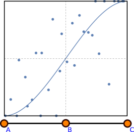
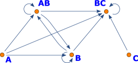
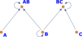
Figure 1. Bottom left: A simplicial complex in $\mathbb{R}$ whose polytope is the interval $[0,1]$. Left: A map $f:[0,1]\ni x\mapsto 3x^{2}-2x^{3}\in[0,1]$ and a sample of $f$ with large Gaussian noise. Middle and right: The constructed combinatorial dynamical system $F_{\mu}$ with threshold $\mu=0.3$ (middle) and $\mu=0.4$ (right).

3.4. A digraph interpretation of a combinatorial dynamical system

A combinatorial dynamical system $F$ may be viewed as a digraph $G_{F}$ whose vertices are simplices in $K$ with a directed edge from $\sigma$ to $\tau$ if and only if $\tau\in F(\sigma)$. An example is presented in Figure 1. The polytope is the interval $[0,1]\subseteq\mbox{$\mathbb{R}$}$. The simplicial complex $K$ (see Figure 1(bottom left)) consists of two toplexes $\mathbf{A}$$\mathbf{B}$ and $\mathbf{B}$$\mathbf{C}$ and three vertices $\mathbf{A}$, $\mathbf{B}$, $\mathbf{C}$ where $\mathbf{A}$, $\mathbf{B}$, $\mathbf{C}$ are points in $\mathbb{R}$ with coordinates $0$, $\frac{1}{2}$ and $1$ respectively. A map $f:[0,1]\to[0,1]$ and a noisy sample of this map are presented in Figure 1(left). The relative freqencies are $\bar{n}_{AB,AB}=\frac{11}{12}$, $\bar{n}_{AB,BC}=\frac{4}{12}$, $\bar{n}_{BC,AB}=\frac{3}{12}$ and $\bar{n}_{BC,BC}=1$. Figure 1(middle) and Figure 1(right) show digraph presentations of two combinatorial dynamical systems on $K$ respectively for thresholds $\mu=0.3$ and $\mu=0.4$. In order to explain the presence of the loop at vertex $\mathbf{B}$ notice that $\mathbf{B}$ is a face of two toplexes: $\mathbf{A}$$\mathbf{B}$ and $\mathbf{B}$$\mathbf{C}$. For thresholds $\mu\in\{0.3,0.4\}$ we have $\text{$\mathbf{A}$}\text{$\mathbf{B}$}\in A_{\mu,\text{$\mathbf{A}$}\text{$\mathbf{B}$}}$ and $\text{$\mathbf{B}$}\text{$\mathbf{C}$}\in A_{\mu,\text{$\mathbf{B}$}\text{$\mathbf{C}$}}$. Therefore, $F_{\mu}(\text{$\mathbf{B}$})=\operatorname{co}\{\text{$\mathbf{A}$}\text{$\mathbf{B}$},\text{$\mathbf{B}$}\text{$\mathbf{C}$}\}=\{\text{$\mathbf{A}$}\text{$\mathbf{B}$},\text{$\mathbf{B}$},\text{$\mathbf{B}$}\text{$\mathbf{C}$}\}$. But, an analogous computation for vertex $\mathbf{A}$ gives $F_{\mu}(\text{$\mathbf{A}$})=\operatorname{co}\{\text{$\mathbf{A}$}\text{$\mathbf{B}$}\}=\{\text{$\mathbf{A}$}\text{$\mathbf{B}$}\}$, which means that there is no loop at vertex $\mathbf{A}$. Similarly, we see that there is no loop at vertex $\mathbf{C}$.

The digraph interpretation of a combinatorial dynamical system means that some concepts in dynamics may be translated into concepts in digraphs and vice versa. In this translation a solution to $F$ in $A\subseteq K$ corresponds to a walk in $G_{F}$ through vertices in $A$ and the set $A$ is invariant if every vertex in $A$ is incident to a bi-infinite walk in $G_{F}$ through vertices in $A$. For instance, in Figure 1(middle), the set $\{\text{$\mathbf{A}$}\text{$\mathbf{B}$},\text{$\mathbf{B}$},\text{$\mathbf{B}$}\text{$\mathbf{C}$}\}$ is invariant. Actually, all its subsets are also invariant because of the presence of loops at $\mathbf{A}$$\mathbf{B}$, $\mathbf{B}$ and $\mathbf{B}$$\mathbf{C}$. The same comment applies to Figure 1(right).

We emphasize that, despite the convenience of the language of digraphs, the combinatorial dynamical system $F$ is more than just the digraph $G_{F}$, because the collection of simplices $K$, that is the set of vertices of $G_{F}$, is a $T_{0}$ topological space. In particular, the concept of isolating neighborhood which we define in Section 4.1, cannot be formulated in the language of digraphs only.

3.5. A combinatorial dynamical system from a sampled vector field

When the dynamics which is sampled constitutes a flow, that is when time is continuous as in the case of a differential equation, the sampled data often consists of a cloud of points with a vector attached to every point. In this case the construction of combinatorial dynamical system is done in two steps. In the first step the cloud of vectors is transformed into a combinatorial vector field in the sense of Forman [14, 15] or its generalized version of combinatorial multivector field [25]. We discuss one of the possible algorithms for the first step in Section 7.2. In the second step, the combinatorial multivector field is transformed into a combinatorial dynamical system. In order to explain the second step, we introduce some definitions. Let $K$ be a simplicial complex. We say that $A\subseteq K$ is orderly convex if for any $\sigma_{1},\sigma_{2}\in A$ and $\tau\in K$ the relations $\sigma_{1}\preceq\tau$ and $\tau\preceq\sigma_{2}$ imply $\tau\in A$. We define a multivector as an orderly convex subset of $K$ and a combinatorial multivector field on $K$ (combinatorial multivector field in short) as a partition $\mathcal{V}$ of $K$ into multivectors. Note that this definition of a combinatorial multivector field is less restrictive than the one in [25]. Both definitions encompass the combinatorial vector field of Forman as a special case. The definition of combinatorial multivector field in [25] additionally requires that multivectors have a unique maximal element. This is not needed here.

Given a combinatorial multivector field $\mathcal{V}$, we denote by $[\sigma]_{\text{$\mathcal{V}$}}$ the unique $V$ in $\mathcal{V}$ such that $\sigma\in V$. We associate with $\mathcal{V}$ a combinatorial dynamical system $F_{\text{$\mathcal{V}$}}:K\multimap K$ given by $F_{\text{$\mathcal{V}$}}(\sigma):=\operatorname{cl}\sigma\cup[\sigma]_{\text{$\mathcal{V}$}}.$ Note that $F_{\text{$\mathcal{V}$}}$ in general admits more solutions than $\Pi_{\text{$\mathcal{V}$}}$ defined in [25, Section 5.4]. In particular, each $\sigma\in K$ is a fixed point of $F_{\text{$\mathcal{V}$}}$, that is, $\sigma\in F_{\text{$\mathcal{V}$}}(\sigma)$. This may look like a drawback but actually it simplifies the theory and allows detecting and eliminating spurious fixed points by the triviality of their Conley index [19].

         

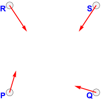
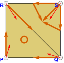
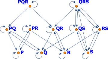
Figure 2. Left: A cloud of vectors. Middle: A possible combinatorial multivector field representation of the cloud of vectors. Right: The associated combinatorial dynamical system represented as a digraph.

Figure 2(left) presents a toy example of a cloud of vectors. It consists of four vectors marked red at four points $\mathbf{P}$, $\mathbf{Q}$, $\mathbf{R}$, $\mathbf{S}$. One of possible geometric simplicial complexes with vertices at points $\mathbf{P}$, $\mathbf{Q}$, $\mathbf{R}$, $\mathbf{S}$ is the simplicial complex $K$ consisting of triangles $\mathbf{P}$$\mathbf{Q}$$\mathbf{R}$, $\mathbf{Q}$$\mathbf{R}$$\mathbf{S}$ and its faces. A possible multivector field $\mathcal{V}$ on $K$ constructed from the cloud of vectors consists of multivectors $\{\text{$\mathbf{P}$},\text{$\mathbf{P}$}\text{$\mathbf{R}$}\}$, $\{\text{$\mathbf{R}$},\text{$\mathbf{Q}$}\text{$\mathbf{R}$}\}$, $\{\text{$\mathbf{Q}$},\text{$\mathbf{P}$}\text{$\mathbf{Q}$}\}$, $\{\text{$\mathbf{P}$}\text{$\mathbf{Q}$}\text{$\mathbf{R}$}\}$,$\{\text{$\mathbf{S}$},\text{$\mathbf{R}$}\text{$\mathbf{S}$},\text{$\mathbf{Q}$}\text{$\mathbf{S}$},\text{$\mathbf{Q}$}\text{$\mathbf{R}$}\text{$\mathbf{S}$}\}$. It is indicated in Figure 2(middle) by orange arrows between centers of mass of simplices. Note that in order to keep the figure legible, only arrows in the direction increasing the dimension are marked. The singleton $\{\text{$\mathbf{P}$}\text{$\mathbf{Q}$}\text{$\mathbf{R}$}\}$ is marked with an orange circle. The associated combinatorial dynamical system $F_{\text{$\mathcal{V}$}}$ presented as a digraph is in Figure 2(right). Note that in general $K$ and $\mathcal{V}$ are not uniquely determined by the cloud of vectors. One possible method for constructing combinatorial multivector fields from a cloud of vectors is discussed in Section 7.2.

4. Isolated invariant sets and Morse decompositions

In this section we consider a combinatorial dynamical system $F:X\multimap X$ and define for $F$ the concepts of isolating neighborhood, isolated invariant set and Morse decomposition.

4.1. Isolated invariant sets

The closed set $N\subseteq K$ is an isolating neighborhood for an invariant set $S\subseteq K$ if $S$ is contained in $N$ and any partial solution in $N$ with endpoints in $S$ has all values in $S$. If such an isolating neighborhood for $S$ exists, we say that $S$ is an isolated invariant set. We emphasize that, unlike the classical theory, the same set $N$ may be an isolating neighborhood for more than one isolated invariant set.

The invariant set $\{\text{$\mathbf{A}$}\text{$\mathbf{B}$}\}$ in Figure 1(middle) is not an isolated invariant set, because for any closed set $N$ containing $\{\text{$\mathbf{A}$}\text{$\mathbf{B}$}\}$ the partial solution $(\text{$\mathbf{A}$}\text{$\mathbf{B}$},\text{$\mathbf{B}$},\text{$\mathbf{A}$}\text{$\mathbf{B}$})$ is contained in $N$ and has endpoints in $\{\text{$\mathbf{A}$}\text{$\mathbf{B}$}\}$. The invariant sets $\{\text{$\mathbf{B}$}\text{$\mathbf{C}$}\}$ and $\{\text{$\mathbf{A}$}\text{$\mathbf{B}$},\text{$\mathbf{B}$}\}$ are both isolated invariant sets and $\{\text{$\mathbf{A}$},\text{$\mathbf{A}$}\text{$\mathbf{B}$},\text{$\mathbf{B}$},\text{$\mathbf{B}$}\text{$\mathbf{C}$},\text{$\mathbf{C}$}\}$ is an isolating neighborhood for both.

Since we have a loop at every vertex of the digraph of the combinatorial dynamical system in Figure 2(right), every set is invariant. In particular, every singleton is invariant. However, the only singleton which is an isolated invariant set is $\{\text{$\mathbf{P}$}\text{$\mathbf{Q}$}\text{$\mathbf{R}$}\}$. Its isolating neighborhood is $\operatorname{cl}\{\text{$\mathbf{P}$}\text{$\mathbf{Q}$}\text{$\mathbf{R}$}\}=\{\text{$\mathbf{P}$},\text{$\mathbf{Q}$},\text{$\mathbf{R}$},\text{$\mathbf{P}$}\text{$\mathbf{Q}$},\text{$\mathbf{P}$}\text{$\mathbf{R}$},\text{$\mathbf{Q}$}\text{$\mathbf{R}$},\text{$\mathbf{P}$}\text{$\mathbf{Q}$}\text{$\mathbf{R}$}\}$. Another isolated invariant set with the same isolating neighborhood is $\{\text{$\mathbf{P}$}\text{$\mathbf{Q}$},\text{$\mathbf{P}$}\text{$\mathbf{R}$},\text{$\mathbf{Q}$}\text{$\mathbf{R}$}\}$.

The maximal invariant set of $F$, denoted $S(F)$, is the set of all simplices $\sigma\in K$ such that there exists a full solution of $F$ in $K$ passing through $\sigma$. It is straightforward to observe that $S(F)$ is invariant and $K$ is an isolating neighborhood for $S(F)$. Therefore, $S(F)$ is an isolated invariant set. Note that the maximal invariant set $S(F_{\text{$\mathcal{V}$}})$ for a combinatorial multivector field $\mathcal{V}$ is always the whole $K$, because for each $\sigma\in K$ we have $\sigma\in\operatorname{cl}\sigma\subseteq F_{\text{$\mathcal{V}$}}(\sigma)$. This is visible in Figure 2(right) as a loop at every vertex. In contrast, $\mathbf{A}$ does not belong to the maximal invariant set in Figure 1(right).

4.2. Morse decompositions

A connection from an isolated invariant set $S_{1}$ to an isolated invariant set $S_{2}$ is a partial solution with left endpoint in $S_{1}$ and right endpoint in $S_{2}$. A family $\mathcal{M}$ consisting of mutually disjoint, non-empty isolated invariant subsets of an isolated invariant set $S$ is a Morse decomposition of $S$ if $\mathcal{M}$ admits a partial order $\leq$ such that any connection between elements in $\mathcal{M}$ either has all values in a single element of $\mathcal{M}$ or it originates in $M\in\text{$\mathcal{M}$}$ and terminates in $M^{\prime}$ such that $M>M^{\prime}$. If $S$ is not mentioned explicitly, we mean a Morse decomposition of the maximal invariant set $S(F)$. The elements of $\mathcal{M}$ are called Morse sets. Although the definitions of isolated invariant set and Morse decomposition require topology, there is an important case when they correspond to purely graph-theoretic concepts. An isolated invariant set is minimal if it admits no non-trivial Morse decomposition that is no Morse decomposition consisting of more than one Morse set. A Morse decomposition is minimal if each of its Morse sets is minimal. The following theorem shows that the minimal Morse decomposition of $F$, denoted as $\text{$\mathcal{M}$}(F)$, is unique and consists of the strongly connected components of $G_{F}$.

Theorem 4.1.

The family of all strongly connected components of $G_{F}$ is the unique minimal Morse decomposition of $S(F)$.

Proof:  Let $\mathcal{S}$ be the family of all strongly connected components of $G_{F}$. We will show that $K$ is an isolating neighborhood for any $S\in\text{$\mathcal{S}$}$. Obviously, $K$, as the whole space is closed. Therefore, $S\subseteq K$. Moreover, any partial solution with endpoints in $S$ must have all values in $S$, because $S$ is a strongly connected component of $G_{F}$. Hence, each $S\in\text{$\mathcal{S}$}$ is an isolated invariant set. Clearly, it is a minimal isolated invariant set. For $S_{1},S_{2}\in\text{$\mathcal{S}$}$ we write $S_{1}\geq S_{2}$ if the there exists a connection from $S_{1}$ to $S_{2}$. Since $\mathcal{S}$ consists of strongly connected components, this defines a partial order on $\mathcal{S}$. Let $\rho$ be a connection from $S_{1}$ to $S_{2}$ whose values are not contained in a single element of $\mathcal{S}$. Then, $S_{1}>S_{2}$. This proves that $\mathcal{S}$ is a Morse decomposition. Obviously, a strongly connected component cannot have a non-trivial Morse decomposition. Thus, $\mathcal{S}$ is a minimal Morse decomposition. Assume that $\text{$\mathcal{S}$}^{\prime}$ is another minimal Morse decomposition and $S^{\prime}\in\text{$\mathcal{S}$}^{\prime}$. We claim that $S^{\prime}$ is strongly connected as a subgraph of $G_{F}$. Indeed, if not, then, according to what we already proved, the strongly connected components of $S^{\prime}$ would constitute a non-trivial Morse decomposition of $S^{\prime}$, contradicting the assumption that $S^{\prime}$ is a minimal invariant set. Hence, $S^{\prime}$ is contained in a Morse set $S\in\text{$\mathcal{S}$}$. By a symmetric argument every $S\in\text{$\mathcal{S}$}$ is contained in a Morse set $S^{\prime}\in\text{$\mathcal{S}$}^{\prime}$. This shows that $\text{$\mathcal{S}$}=\text{$\mathcal{S}$}^{\prime}$ and proves the uniqueness. ∎

Figure 3. Left: The minimal Morse decomposition of the combinatorial dynamical system in Figure 1(middle) consisting of $\{\text{$\mathbf{A}$}\text{$\mathbf{B}$},\text{$\mathbf{B}$}\}$ (green) and $\{\text{$\mathbf{B}$}\text{$\mathbf{C}$}\}$ (blue). Middle: The minimal Morse decomposition of the combinatorial dynamical system in Figure 1(right) consisting of $\{\text{$\mathbf{A}$}\text{$\mathbf{B}$}\}$ (green), $\{\text{$\mathbf{B}$}\}$ (yellow) and $\{\text{$\mathbf{B}$}\text{$\mathbf{C}$}\}$ (blue). Right: The minimal Morse decomposition of the combinatorial dynamical system in Figure 2(right) consisting of $\{\text{$\mathbf{P}$},\text{$\mathbf{Q}$},\text{$\mathbf{R}$},\text{$\mathbf{P}$}\text{$\mathbf{Q}$},\text{$\mathbf{P}$}\text{$\mathbf{R}$},\text{$\mathbf{Q}$}\text{$\mathbf{R}$}\}$ (yellow), $\{\text{$\mathbf{S}$},\text{$\mathbf{R}$}\text{$\mathbf{S}$},\text{$\mathbf{Q}$}\text{$\mathbf{S}$},\text{$\mathbf{Q}$}\text{$\mathbf{R}$}\text{$\mathbf{S}$}\}$ (green) and $\{\text{$\mathbf{P}$}\text{$\mathbf{Q}$}\text{$\mathbf{R}$}\}$ (blue).

Consider the combinatorial dynamical system in Figure 1(middle). Its minimal Morse decomposition consists of two Morse sets: $\{\text{$\mathbf{A}$}\text{$\mathbf{B}$},\text{$\mathbf{B}$}\}$ and $\{\text{$\mathbf{B}$}\text{$\mathbf{C}$}\}$ with $\{\text{$\mathbf{A}$}\text{$\mathbf{B}$},\text{$\mathbf{B}$}\}>\{\text{$\mathbf{B}$}\text{$\mathbf{C}$}\}$. The minimal Morse decomposition of the combinatorial dynamical system in Figure 1(right) consists of three Morse sets: $\{\text{$\mathbf{A}$}\text{$\mathbf{B}$}\}$, $\{\text{$\mathbf{B}$}\}$ and $\{\text{$\mathbf{B}$}\text{$\mathbf{C}$}\}$ with $\{\text{$\mathbf{B}$}\}>\{\text{$\mathbf{B}$}\text{$\mathbf{C}$}\}$ and $\{\text{$\mathbf{B}$}\}>\{\text{$\mathbf{A}$}\text{$\mathbf{B}$}\}$. The minimal Morse decomposition of the combinatorial dynamical system in Figure 2(right) consists of three isolated invariant sets: $M_{1}:=\{\text{$\mathbf{P}$},\text{$\mathbf{Q}$},\text{$\mathbf{R}$},\text{$\mathbf{P}$}\text{$\mathbf{Q}$},\text{$\mathbf{P}$}\text{$\mathbf{R}$},\text{$\mathbf{Q}$}\text{$\mathbf{R}$}\}$, $M_{2}:=\{\text{$\mathbf{S}$},\text{$\mathbf{R}$}\text{$\mathbf{S}$},\text{$\mathbf{Q}$}\text{$\mathbf{S}$},\text{$\mathbf{Q}$}\text{$\mathbf{R}$}\text{$\mathbf{S}$}\}$ and $M_{3}:=\{\text{$\mathbf{P}$}\text{$\mathbf{Q}$}\text{$\mathbf{R}$}\}$ with $M_{3}>M_{1}$ and $M_{2}>M_{1}$. These minimal Morse decompositions are illustrated in Figure 3.

5. Persistence of Morse decompositions.

In this section we define homological persistence of Morse decompositions in the setting of combinatorial dynamical systems.

5.1. Disconnecting topology.

In the case of a classical Morse decomposition consisting of more than one Morse set, the union of all Morse sets is always disconnected in the topology induced from the space. This is because Morse sets are always disjoint and in this case also compact. In particular, the space between the Morse sets is filled with solutions connecting the Morse sets. But, in finite topological spaces the Morse sets need not be closed and solutions may jump directly from one Morse set to another Morse set. Consequently, the union of Morse sets generally is not disconnected. Thus, we need a method to disconnect Morse sets. Fortunately, in this case we do not need space between the Morse sets. We achieve the separation by purely topological methods. To explain this, we need the following terminology, notation and theorem.

Assume $\mathcal{A}$ is a finite family of mutually disjoint non-empty sets and $\mathcal{T}$ is a topology on $\bigcup\text{$\mathcal{A}$}$. We say that $\mathcal{A}$ is disconnected in $\mathcal{T}$ if each set $A\in\text{$\mathcal{A}$}$ is open in the topology $\mathcal{T}$.

Given a family $\mathcal{A}$ of subsets of a set $X$, we use the notation $\text{$\mathcal{A}$}^{*}:=\{\bigcup\text{$\mathcal{A}$}^{\prime}:\text{$\mathcal{A}$}^{\prime}\subseteq\text{$\mathcal{A}$}\}$ for the smallest family of sets in $X$, containing $\mathcal{A}$ and closed under summation. If $\mathcal{B}$ is another such family, we write $\text{$\mathcal{A}$}\mathbin{\bar{\cap}}\text{$\mathcal{B}$}$ for the family of intersections of every set in $\mathcal{A}$ with every set in $\mathcal{B}$. We say that $\mathcal{A}$ is inscribed in $\mathcal{B}$ and write $\text{$\mathcal{A}$}\sqsubset\text{$\mathcal{B}$}$ if for every $A\in\text{$\mathcal{A}$}$, there exists a $B\in\text{$\mathcal{B}$}$ such that $A\subseteq B$.

In order to shorten the notation we will also write $\langle\text{$\mathcal{A}$}\rangle$ for the union $\bigcup\text{$\mathcal{A}$}$ of all the sets in $\mathcal{A}$. Note that if $A\subseteq X$ and $\mathcal{T}$ is a topology on $X$, then the topology induced by $\mathcal{T}$ on $A$ is $A\mathbin{\bar{\cap}}\text{$\mathcal{T}$}:=\{A\}\mathbin{\bar{\cap}}\text{$\mathcal{T}$}$.

Theorem 5.1.

Assume $(X,\text{$\mathcal{T}$})$ is an arbitrary topological space and $\mathcal{A}$ is a finite family of mutually disjoint, non-empty subsets of $X$. Then $\text{$\mathcal{T}$}_{\text{$\mathcal{A}$}}:=\left(\text{$\mathcal{A}$}\mathbin{\bar{\cap}}\text{$\mathcal{T}$}\right)^{*}$ is a topology on $\langle\text{$\mathcal{A}$}\rangle$. Moreover,

• if $\mathcal{T}$ is a $T_{0}$ topology, then so is $\text{$\mathcal{T}$}_{\text{$\mathcal{A}$}}$,

• for every $A\in\text{$\mathcal{A}$}$, the topology induced on $A$ by $\mathcal{T}$ coincides with the topology induced on $A$ by $\text{$\mathcal{T}$}_{\text{$\mathcal{A}$}}$,

• the family $\mathcal{A}$ is $\text{$\mathcal{T}$}_{\text{$\mathcal{A}$}}$-disconnected,

• if additionally $\langle\text{$\mathcal{A}$}\rangle=X$ and each set in $\mathcal{A}$ is $\mathcal{T}$-connected, then the connected components with respect to $\text{$\mathcal{T}$}_{\text{$\mathcal{A}$}}$ coincide with the sets in $\mathcal{A}$.

Proof:  We will show that $\text{$\mathcal{A}$}\mathbin{\bar{\cap}}\text{$\mathcal{T}$}$ is a basis (see [28, Section 13]) for some topology on $\langle\text{$\mathcal{A}$}\rangle$. Let $x\in\langle\text{$\mathcal{A}$}\rangle$. There exists an $A\in\text{$\mathcal{A}$}$ such that $x\in A$. Hence, $x\in A=A\cap X\in\text{$\mathcal{A}$}\mathbin{\bar{\cap}}\text{$\mathcal{T}$}$. Assume that $x\in(A\cap U)\cap(B\cap V)$ for some $A,B\in\text{$\mathcal{A}$}$ and $U,V\in\text{$\mathcal{T}$}$. Then $A=B$ and consequently $(A\cap U)\cap(B\cap V)=A\cap(U\cap V)\in\text{$\mathcal{A}$}\mathbin{\bar{\cap}}\text{$\mathcal{T}$}$. This shows that $\text{$\mathcal{A}$}\mathbin{\bar{\cap}}\text{$\mathcal{T}$}$ is indeed a basis. By [28, 13.1] it follows that $\text{$\mathcal{T}$}_{\text{$\mathcal{A}$}}$ is a topology. Consider $x,y\in\langle\text{$\mathcal{A}$}\rangle$, $x\neq y$. Without loss of generality we can assume that there exists an open neighbourhood $U\in\text{$\mathcal{T}$}$ of $y$ such that $x\not\in U$. Let $A\in\text{$\mathcal{A}$}$ be such that $y\in A$. Then $y\in U\cap A$ and $x\not\in U\cap A$, hence (i) holds. To prove (ii) we need to show that $A\mathbin{\bar{\cap}}\text{$\mathcal{T}$}=A\mathbin{\bar{\cap}}\text{$\mathcal{T}$}_{\text{$\mathcal{A}$}}$. Obviously $A\mathbin{\bar{\cap}}\text{$\mathcal{T}$}\subseteq A\mathbin{\bar{\cap}}\text{$\mathcal{T}$}_{\text{$\mathcal{A}$}}$. To prove the opposite inclusion take a $V\in A\mathbin{\bar{\cap}}\text{$\mathcal{T}$}_{\text{$\mathcal{A}$}}$. This means that there is a $U\in\text{$\mathcal{T}$}_{\text{$\mathcal{A}$}}$ such that $V=A\cap U$. Then $U=\bigcup_{i\in I}(A_{i}\cap U_{i})$ for some $U_{i}\in\text{$\mathcal{T}$}$ and $A_{i}\in\text{$\mathcal{A}$}$. Hence $V=A\cap U=A\cap\bigcup_{i\in I}(A_{i}\cap U_{i})=A\cap\bigcup_{i\in I_{A}}U_{i}\in A\mathbin{\bar{\cap}}\text{$\mathcal{T}$}$ where $I_{A}=\{i\in I:A_{i}=A\}$ and (ii) is proved. Property (iii) is obvious, because $A\in\text{$\mathcal{A}$}$ implies $A=A\cap X\in\text{$\mathcal{T}$}_{\text{$\mathcal{A}$}}$. To prove (iv) assume $A$ is $\mathcal{T}$-connected. It follows from (ii) that $A$ is $\text{$\mathcal{T}$}_{\text{$\mathcal{A}$}}$-connected. Let $x\in A$. Then $A$ is contained in $[x]_{\text{$\mathcal{T}$}_{\text{$\mathcal{A}$}}}$, the $\text{$\mathcal{T}$}_{\text{$\mathcal{A}$}}$-connected component of $x$. This means that $[x]_{\text{$\mathcal{T}$}_{\text{$\mathcal{A}$}}}=\bigcup\text{$\mathcal{A}$}^{\prime}$ for some $\text{$\mathcal{A}$}^{\prime}\subseteq\text{$\mathcal{A}$}$. Since every set in $\mathcal{A}$ is open in $\text{$\mathcal{T}$}_{\text{$\mathcal{A}$}}$, the family $\text{$\mathcal{A}$}^{\prime}$ must contain precisely one element. Consequently $A=[x]_{\text{$\mathcal{T}$}_{\text{$\mathcal{A}$}}}$ and (iv) holds. ∎

We note that given a Morse decomposition $\mathcal{M}$ of a combinatorial dynamical system $F$ on a finite simplicial complex $K$, in general the union $\langle\text{$\mathcal{M}$}\rangle$ is not a subcomplex of the simplicial complex $K$. Therefore, we cannot take simplicial homology of $\langle\text{$\mathcal{M}$}\rangle$. Moreover, we are interested in the special topology $\text{$\mathcal{T}$}_{\text{$\mathcal{M}$}}$ on $\langle\text{$\mathcal{M}$}\rangle$ where $\mathcal{T}$ is the Alexandrov topology of $K$. The topology $\text{$\mathcal{T}$}_{\text{$\mathcal{M}$}}$ separates the Morse sets due to Theorem 5.1(iii). Fortunately, the singular homology makes sense for any topological space, in particular we can consider $H(\langle\text{$\mathcal{M}$}\rangle,\text{$\mathcal{T}$}_{\text{$\mathcal{M}$}})$. In Section 6 we use McCord’s Theorem [21] to show that $H(\langle\text{$\mathcal{M}$}\rangle,\text{$\mathcal{T}$}_{\text{$\mathcal{M}$}})$ may be computed as simplicial homology of a subcomplex of the barycentric subdivision of $K$.

5.2. Persistence and zig-zag persistence of Morse decompositions

Consider two simplicial complexes $K$ and $K^{\prime}$ with combinatorial dynamical systems $F$ on $K$ and $F^{\prime}$ on $K^{\prime}$ and a map $f:K\to K^{\prime}$ continuous with respect to Alexandrov topologies $\mathcal{T}$ on $K$ and $\text{$\mathcal{T}$}^{\prime}$ on $K^{\prime}$. By Theorem 2.1 (Alexandrov Theorem) the map $f$ is continuous if and only if it preserves the face relation in $K$ and $K^{\prime}$. In particular, every simplicial map is continuous.

The following theorem lets us define homomorphisms in homology needed to set up persistence of Morse decompositions.

Theorem 5.2.

Let $\mathcal{M}$ and $\text{$\mathcal{M}$}^{\prime}$ be Morse decompositions respectively for $F$ and $F^{\prime}$. Assume that continuous map $f:K\to K^{\prime}$ respects $\mathcal{M}$ and $\text{$\mathcal{M}$}^{\prime}$ that is $f(\text{$\mathcal{M}$})\sqsubset\text{$\mathcal{M}$}^{\prime}$ where $f(\text{$\mathcal{M}$}):=\mbox{$\{\,f(M)\mid M\in\text{$\mathcal{M}$}\,\}$}$. Then, the map $f_{\text{$\mathcal{M}$},\text{$\mathcal{M}$}^{\prime}}:(\langle\text{$\mathcal{M}$}\rangle,\text{$\mathcal{T}$}_{\text{$\mathcal{M}$}})\ni\sigma\mapsto f(\sigma)\in(\langle\text{$\mathcal{M}$}^{\prime}\rangle,\text{$\mathcal{T}$}^{\prime}_{\text{$\mathcal{M}$}^{\prime}})$ is well defined and continuous.

Proof:  Let $\sigma\in\langle\text{$\mathcal{M}$}\rangle$. Then $\sigma\in M$ for some $M\in\text{$\mathcal{M}$}$. Since $f$ respects $\mathcal{M}$ and $\text{$\mathcal{M}$}^{\prime}$, there is an $M^{\prime}\in\text{$\mathcal{M}$}^{\prime}$ such that $f(M)\subseteq M^{\prime}$. It follows that $f(\sigma)\in\langle\text{$\mathcal{M}$}^{\prime}\rangle$. Hence, $f_{\text{$\mathcal{M}$},\text{$\mathcal{M}$}^{\prime}}$ is well defined. Since $\text{$\mathcal{M}$}^{\prime}\mathbin{\bar{\cap}}\text{$\mathcal{T}$}^{\prime}$ is a basis of topology $\text{$\mathcal{T}$}^{\prime}_{\text{$\mathcal{M}$}^{\prime}}$, in order to prove continuity it suffices to show that for any $M^{\prime}\in\text{$\mathcal{M}$}^{\prime}$ and $T^{\prime}\in\text{$\mathcal{T}$}^{\prime}$ the set $f_{\text{$\mathcal{M}$},\text{$\mathcal{M}$}^{\prime}}^{-1}(M^{\prime}\cap T^{\prime})$ is open in $\text{$\mathcal{T}$}_{\text{$\mathcal{M}$}}$. Let $\text{$\mathcal{M}$}_{M^{\prime}}:=\mbox{$\{\,M\in\text{$\mathcal{M}$}\mid f(M)\subseteq M^{\prime}\,\}$}$. Then $f^{-1}(M^{\prime})\cap\langle\text{$\mathcal{M}$}\rangle=\langle\text{$\mathcal{M}$}_{M^{\prime}}\rangle$. By continuity of $f$ we have $f^{-1}(T^{\prime})\in\text{$\mathcal{T}$}$. Therefore, $f_{\text{$\mathcal{M}$},\text{$\mathcal{M}$}^{\prime}}^{-1}(M^{\prime}\cap T^{\prime})=f^{-1}(M^{\prime})\cap f^{-1}(T^{\prime})\cap\langle\text{$\mathcal{M}$}\rangle=f^{-1}(T^{\prime})\cap\langle\text{$\mathcal{M}$}_{M^{\prime}}\rangle=\bigcup\{M\cap f^{-1}(T^{\prime})\mid M\in\text{$\mathcal{M}$}_{M^{\prime}}\}\in(\text{$\mathcal{M}$}\mathbin{\bar{\cap}}\text{$\mathcal{T}$})^{*}=\text{$\mathcal{T}$}_{\text{$\mathcal{M}$}},$ which completes the proof. ∎

For a minimal Morse decomposition, denoted by $\text{$\mathcal{M}$}(F)$, we have the following corollary.

Corollary 5.3.

The map $f_{\text{$\mathcal{M}$}(F),\text{$\mathcal{M}$}(F^{\prime})}:(\langle\text{$\mathcal{M}$}(F)\rangle,\text{$\mathcal{T}$}_{\text{$\mathcal{M}$}(F)})\to(\langle\text{$\mathcal{M}$}(F^{\prime})\rangle,\text{$\mathcal{T}$}^{\prime}_{\text{$\mathcal{M}$}(F^{\prime})})$ is continuous under the assumption that $f\circ F\subseteq F^{\prime}\circ f$ that is $f(F(\sigma))\subseteq F^{\prime}(f(\sigma))$ for any $\sigma\in K$.

Proof:  By Theorem 5.2, it suffices to show that $f$ respects $\text{$\mathcal{M}$}(F)$ and $\text{$\mathcal{M}$}(F^{\prime})$. Let $M\in\text{$\mathcal{M}$}(F)$. By Theorem 4.1, the Morse set $M$ is a strongly connected component of $G_{F}$. Let $\sigma,\tau\in M$ and let $\rho$ be a partial solution in $M$ with endpoints $\sigma$ and $\tau$. It follows from the assumption that $f\circ\rho$ is a solution in $f(M)$ with endpoints $f(\sigma)$ and $f(\tau)$. Since $\sigma,\tau\in M$ are arbitrary, the set $f(M)$ must be contained in one strongly connected component of $G_{F^{\prime}}$, that is $f(M)\subseteq M^{\prime}$ for some $M^{\prime}\in\text{$\mathcal{M}$}^{\prime}$. ∎

Assume now that for $i=1,2,\ldots n$, we have a simplicial complex $K_{i}$ with Alexandrov topology $\text{$\mathcal{T}$}^{i}$, a combinatorial dynamical system $F_{i}$ on $K_{i}$, and a Morse decomposition $\text{$\mathcal{M}$}_{i}$ of $F_{i}$. Let $\{f_{i}:K_{i}\to K_{i+1}\}_{i=1,n-1}$ be a sequence of continuous maps such that $f_{i}\circ F_{i}\subseteq F_{i+1}\circ f_{i}$ and $f_{i}(\text{$\mathcal{M}$}_{i})\sqsubset\text{$\mathcal{M}$}_{i+1}$. Note that by Corollary 5.3 the latter condition may be dropped if $\text{$\mathcal{M}$}_{i}=\text{$\mathcal{M}$}(F_{i})$. It follows from Theorem 5.2 that the maps $\bar{f}_{i}:=(f_{i})_{\text{$\mathcal{M}$}_{i},\text{$\mathcal{M}$}_{i+1}}:(\langle\text{$\mathcal{M}$}_{i}\rangle,\text{$\mathcal{T}$}^{i}_{\text{$\mathcal{M}$}_{i}})\to(\langle\text{$\mathcal{M}$}_{i+1}\rangle,\text{$\mathcal{T}$}^{i+1}_{\text{$\mathcal{M}$}_{i+1}})$ are continuous. Thus, we have homomorphisms induced in singular homology $H(\bar{f}_{i}):H(\langle\text{$\mathcal{M}$}_{i}\rangle,\text{$\mathcal{T}$}^{i}_{\text{$\mathcal{M}$}_{i}})\to H(\langle\text{$\mathcal{M}$}_{i+1}\rangle,\text{$\mathcal{T}$}^{i+1}_{\text{$\mathcal{M}$}_{i+1}})$. This yields a persistence module

(2)

We refer to the persistence diagram of this module as the persistence diagram of Morse decompositions. We note that zig-zag persistence diagram of Morse decompositions may be obtained analogously by replacing, whenever appropriate, inclusions $f_{i}\circ F_{i}\subseteq F_{i+1}\circ f_{i}$ by $f_{i}\circ F_{i}\supseteq F_{i+1}\circ f_{i}$ and respectively $\bar{f}_{i}(\text{$\mathcal{M}$}_{i})\sqsubset\text{$\mathcal{M}$}_{i+1}$ by $\text{$\mathcal{M}$}_{i}\sqsupset\bar{f}_{i}(\text{$\mathcal{M}$}_{i+1})$.

5.3. Persistence in combinatorial multivector fields

Let $\mathcal{V}$ be a combinatorial multivector field on a simplicial complex $K$. We say that $\mathcal{M}$ is a Morse decomposition of $\mathcal{V}$ if it is a Morse decomposition of the associated combinatorial dynamical system $F_{\text{$\mathcal{V}$}}$. We extend this terminology to minimal Morse decompositions. We denote the minimal Morse decomposition of $\mathcal{V}$ by $\text{$\mathcal{M}$}(\text{$\mathcal{V}$}):=\text{$\mathcal{M}$}(F_{\text{$\mathcal{V}$}})$ and the topology of this Morse decomposition by $\text{$\mathcal{T}$}_{\text{$\mathcal{V}$}}:=\text{$\mathcal{T}$}_{\text{$\mathcal{M}$}(\text{$\mathcal{V}$})}$.

Theorem 5.4.

Morse decompositions of combinatorial multivector fields have the following properties.

• The minimal Morse decomposition of a combinatorial multivector field $\mathcal{V}$ on $K$ is a partition of $K$. In particular, $\langle\text{$\mathcal{M}$}\rangle=K$.

• Given $\mathcal{W}$, another combinatorial multivector field on $K$, the family $\text{$\mathcal{V}$}\mathbin{\bar{\cap}}\text{$\mathcal{W}$}$ is a combinatorial multivector field on $K$. It is inscribed both in $\mathcal{V}$ and $\mathcal{W}$. Moreover, If $\text{$\mathcal{V}$}\sqsubset\text{$\mathcal{W}$}$, then $F_{\text{$\mathcal{V}$}}\subseteq F_{\text{$\mathcal{W}$}}$.

• If $\text{$\mathcal{V}$}^{\prime}$ is a combinatorial multivector field on a simplicial complex $K^{\prime}$ and $f:K\to K^{\prime}$ is continuous, then $f^{*}(\text{$\mathcal{V}$}^{\prime}):=\mbox{$\{\,f^{-1}(V^{\prime})\mid V^{\prime}\in\text{$\mathcal{V}$}^{\prime}\,\}$},$ called the pullback of $\text{$\mathcal{V}$}^{\prime}$, is a combinatorial multivector field on $K$.

• The maps $\kappa:=\operatorname{id}_{\text{$\mathcal{V}$}\mathbin{\bar{\cap}}f^{*}(\text{$\mathcal{V}$}^{\prime}),\text{$\mathcal{V}$}}:(K,\text{$\mathcal{T}$}_{\text{$\mathcal{V}$}\mathbin{\bar{\cap}}f^{*}(\text{$\mathcal{V}$}^{\prime})})\to(K,\text{$\mathcal{T}$}_{\text{$\mathcal{V}$}})$ induced by identity and $\lambda:=f_{\text{$\mathcal{V}$}\mathbin{\bar{\cap}}f^{*}(\text{$\mathcal{V}$}^{\prime}),\text{$\mathcal{V}$}^{\prime}}:(K,\text{$\mathcal{T}$}_{\text{$\mathcal{V}$}\mathbin{\bar{\cap}}f^{*}(\text{$\mathcal{V}$}^{\prime})})\to(K^{\prime},\text{$\mathcal{T}$}^{\prime}_{\text{$\mathcal{V}$}^{\prime}})$ induced by $f$ are continuous.

Proof:  Note that by Theorem 4.1, the Morse sets in the minimal Morse decomposition are the strongly connected components of $G_{F_{\text{$\mathcal{V}$}}}$. Hence, to prove (i) it suffices to observe that every $\sigma\in K$ belongs to a strongly connected component. This is obvious because $\sigma\in\operatorname{cl}\sigma\subseteq F_{\text{$\mathcal{V}$}}(\sigma)$ for any $\sigma\in K$. Thus, (i) is proved. Since the intersection of two orderly convex sets is easily seen to be orderly convex, each element of $\text{$\mathcal{V}$}\mathbin{\bar{\cap}}\text{$\mathcal{W}$}$ is orderly convex. Obviously, $\text{$\mathcal{V}$}\mathbin{\bar{\cap}}\text{$\mathcal{W}$}$ is a partition of $K$ and is inscribed in $\mathcal{V}$ and $\mathcal{W}$. Take $\sigma\in K$. Assumption $\text{$\mathcal{V}$}\sqsubset\text{$\mathcal{W}$}$ implies that $[\sigma]_{\text{$\mathcal{V}$}}\subseteq[\sigma]_{\text{$\mathcal{W}$}}$. It follows that $F_{\text{$\mathcal{V}$}}(\sigma)=\operatorname{cl}\sigma\cup[\sigma]_{\text{$\mathcal{V}$}}\subseteq\operatorname{cl}\sigma\cup[\sigma]_{\text{$\mathcal{W}$}}=F_{\text{$\mathcal{W}$}}(\sigma)$. Thus, (ii) is also proved. Obviously, $f^{*}(\text{$\mathcal{V}$}^{\prime})$ is a partition of $K$. To show that for every $V^{\prime}\in\text{$\mathcal{V}$}^{\prime}$ the set $f^{-1}(V^{\prime})$ is orderly convex, take $\sigma,\sigma^{\prime}\in f^{-1}(V^{\prime})$ and $\tau\in K$ such that $\sigma\preceq\tau\preceq\sigma^{\prime}$. Then $f(\sigma),f(\sigma^{\prime})\in V^{\prime}$, $f(\sigma)\preceq f(\tau)\preceq f(\sigma^{\prime})$, and since $V^{\prime}$ is orderly convex, we get $f(\tau)\in V^{\prime}$. It follows that $\tau\in f^{-1}(V^{\prime})$ and $f^{-1}(V^{\prime})$ is orderly convex. This proves (iii). To prove (iv), we verify that the maps $\kappa$ and $\lambda$ satisfy the assumption of Corollary 5.3. It follows from (ii) that $\operatorname{id}\circ F_{\text{$\mathcal{V}$}\mathbin{\bar{\cap}}f^{*}(\text{$\mathcal{V}$}^{\prime})}=F_{\text{$\mathcal{V}$}\mathbin{\bar{\cap}}f^{*}(\text{$\mathcal{V}$}^{\prime})}\subseteq F_{\text{$\mathcal{V}$}}=F_{\text{$\mathcal{V}$}}\circ\operatorname{id}$ which proves that $\kappa$ is continuous. Similarly, we get $f\circ F_{\text{$\mathcal{V}$}\mathbin{\bar{\cap}}f^{*}(\text{$\mathcal{V}$}^{\prime})}\subseteq f\circ F_{f^{*}(\text{$\mathcal{V}$}^{\prime})}.$ Thus, it suffices to prove that $f\circ F_{f^{*}(\text{$\mathcal{V}$}^{\prime})}\subseteq F_{\text{$\mathcal{V}$}^{\prime}}\circ f$. Indeed, for $\sigma\in K$ we get from the continuity of $f$ and the definition of $f^{*}(\text{$\mathcal{V}$}^{\prime})$ that $(f\circ F_{f^{*}(\text{$\mathcal{V}$}^{\prime})})(\sigma)=f(F_{f^{*}(\text{$\mathcal{V}$}^{\prime})}(\sigma))=f(\operatorname{cl}\sigma\cup[\sigma]_{f^{*}(\text{$\mathcal{V}$}^{\prime})})=f(\operatorname{cl}\sigma)\cup f([\sigma]_{f^{*}(\text{$\mathcal{V}$}^{\prime})})\subseteq\operatorname{cl}f(\sigma)\cup[f(\sigma)]_{\text{$\mathcal{V}$}^{\prime}}=F_{\text{$\mathcal{V}$}^{\prime}}(f(\sigma))=(F_{\text{$\mathcal{V}$}^{\prime}}\circ f)(\sigma).$ ∎

We use the diagram of continuous maps referred to as the comparison diagram of combinatorial multivector fields $\mathcal{V}$ and $\text{$\mathcal{V}$}^{\prime}$, to define the persistence of Morse decompositions for combinatorial multivector fields. To this end, assume that, for $i=1,2,\ldots n$, we have a combinatorial multivector field $\text{$\mathcal{V}$}_{i}$ on a simplicial complex $K_{i}$. Moreover, assume that we have a sequence of continuous maps $f_{i}:K_{i}\to K_{i+1}$. Putting together the comparison diagrams of $\text{$\mathcal{V}$}_{i}$ and $\text{$\mathcal{V}$}_{i+1}$ and applying the singular homology functor we obtain the following zig-zag persistence module

(3) $$\lx@xy@svg{\hbox{\raise 0.0pt\hbox{\kern 23.85556pt\hbox{\ignorespaces\ignorespaces\ignorespaces\hbox{\vtop{\kern 0.0pt\offinterlineskip\halign{\entry@#!@&&\entry@@#!@\cr&&&\crcr}}}\ignorespaces{\hbox{\kern-23.85556pt\raise 0.0pt\hbox{\hbox{\kern 0.0pt\raise 0.0pt\hbox{\hbox{\kern 3.0pt\raise 0.0pt\hbox{$\textstyle{H(K_{1},\text{$\mathcal{T}$}^{1}_{\text{$\mathcal{V}$}_{1}})}$}}}}}}}{\hbox{\kern 47.85556pt\raise 0.0pt\hbox{\hbox{\kern 0.0pt\raise 0.0pt\hbox{\hbox{\kern 3.0pt\raise 0.0pt\hbox{$\textstyle{H(K_{1},\text{$\mathcal{T}$}^{1}_{\text{$\mathcal{V}$}_{1}\mathbin{\bar{\cap}}f^{*}(\text{$\mathcal{V}$}_{2})})\ignorespaces\ignorespaces\ignorespaces\ignorespaces\ignorespaces\ignorespaces\ignorespaces\ignorespaces}$}}}}}}}\ignorespaces\ignorespaces\ignorespaces\ignorespaces{}{\hbox{\lx@xy@droprule}}\ignorespaces\ignorespaces\ignorespaces{\hbox{\kern 23.92303pt\raise 6.5pt\hbox{{}\hbox{\kern 0.0pt\raise 0.0pt\hbox{\hbox{\kern 3.0pt\hbox{\hbox{\kern 0.0pt\raise-1.75pt\hbox{$\scriptstyle{H(\kappa_{1})}$}}}\kern 3.0pt}}}}}}\ignorespaces{\hbox{\kern 23.85556pt\raise 0.0pt\hbox{\hbox{\kern 0.0pt\raise 0.0pt\hbox{\lx@xy@tip{1}\lx@xy@tip{-1}}}}}}{\hbox{\lx@xy@droprule}}{\hbox{\lx@xy@droprule}}\ignorespaces\ignorespaces\ignorespaces\ignorespaces{}{\hbox{\lx@xy@droprule}}\ignorespaces\ignorespaces\ignorespaces{\hbox{\kern 95.60904pt\raise 6.5pt\hbox{{}\hbox{\kern 0.0pt\raise 0.0pt\hbox{\hbox{\kern 3.0pt\hbox{\hbox{\kern 0.0pt\raise-1.75pt\hbox{$\scriptstyle{H(\lambda_{1})}$}}}\kern 3.0pt}}}}}}\ignorespaces{\hbox{\kern 119.56668pt\raise 0.0pt\hbox{\hbox{\kern 0.0pt\raise 0.0pt\hbox{\lx@xy@tip{1}\lx@xy@tip{-1}}}}}}{\hbox{\lx@xy@droprule}}{\hbox{\lx@xy@droprule}}{\hbox{\kern 119.56668pt\raise 0.0pt\hbox{\hbox{\kern 0.0pt\raise 0.0pt\hbox{\hbox{\kern 3.0pt\raise 0.0pt\hbox{$\textstyle{H(K_{2},\text{$\mathcal{T}$}^{2}_{\text{$\mathcal{V}$}_{2}})}$}}}}}}}{\hbox{\kern 191.2778pt\raise 0.0pt\hbox{\hbox{\kern 0.0pt\raise 0.0pt\hbox{\hbox{\kern 3.0pt\raise 0.0pt\hbox{$\textstyle{\ldots\ignorespaces\ignorespaces\ignorespaces\ignorespaces}$}}}}}}}\ignorespaces\ignorespaces\ignorespaces\ignorespaces{}{\hbox{\lx@xy@droprule}}\ignorespaces\ignorespaces\ignorespaces{\hbox{\kern 167.34528pt\raise 6.5pt\hbox{{}\hbox{\kern 0.0pt\raise 0.0pt\hbox{\hbox{\kern 3.0pt\hbox{\hbox{\kern 0.0pt\raise-1.75pt\hbox{$\scriptstyle{H(\kappa_{2})}$}}}\kern 3.0pt}}}}}}\ignorespaces{\hbox{\kern 167.2778pt\raise 0.0pt\hbox{\hbox{\kern 0.0pt\raise 0.0pt\hbox{\lx@xy@tip{1}\lx@xy@tip{-1}}}}}}{\hbox{\lx@xy@droprule}}{\hbox{\lx@xy@droprule}}\ignorespaces}}}}\ignorespaces\\ \lx@xy@svg{\hbox{\raise 0.0pt\hbox{\kern 6.75pt\hbox{\ignorespaces\ignorespaces\ignorespaces\hbox{\vtop{\kern 0.0pt\offinterlineskip\halign{\entry@#!@&&\entry@@#!@\cr&&\crcr}}}\ignorespaces{\hbox{\kern-6.75pt\raise 0.0pt\hbox{\hbox{\kern 0.0pt\raise 0.0pt\hbox{\hbox{\kern 3.0pt\raise 0.0pt\hbox{$\textstyle{\ldots}$}}}}}}}{\hbox{\kern 30.75pt\raise 0.0pt\hbox{\hbox{\kern 0.0pt\raise 0.0pt\hbox{\hbox{\kern 3.0pt\raise 0.0pt\hbox{$\textstyle{H(K_{n-1},\text{$\mathcal{T}$}^{n-1}_{\text{$\mathcal{V}$}_{n-1}\mathbin{\bar{\cap}}f^{*}(\text{$\mathcal{V}$}_{n})})\ignorespaces\ignorespaces\ignorespaces\ignorespaces\ignorespaces\ignorespaces\ignorespaces\ignorespaces}$}}}}}}}\ignorespaces\ignorespaces\ignorespaces\ignorespaces{}{\hbox{\lx@xy@droprule}}\ignorespaces\ignorespaces\ignorespaces{\hbox{\kern 6.617pt\raise 6.5pt\hbox{{}\hbox{\kern 0.0pt\raise 0.0pt\hbox{\hbox{\kern 3.0pt\hbox{\hbox{\kern 0.0pt\raise-1.75pt\hbox{$\scriptstyle{H(\kappa_{n})}$}}}\kern 3.0pt}}}}}}\ignorespaces{\hbox{\kern 6.75pt\raise 0.0pt\hbox{\hbox{\kern 0.0pt\raise 0.0pt\hbox{\lx@xy@tip{1}\lx@xy@tip{-1}}}}}}{\hbox{\lx@xy@droprule}}{\hbox{\lx@xy@droprule}}\ignorespaces\ignorespaces\ignorespaces\ignorespaces{}{\hbox{\lx@xy@droprule}}\ignorespaces\ignorespaces\ignorespaces{\hbox{\kern 88.75897pt\raise 6.5pt\hbox{{}\hbox{\kern 0.0pt\raise 0.0pt\hbox{\hbox{\kern 3.0pt\hbox{\hbox{\kern 0.0pt\raise-1.75pt\hbox{$\scriptstyle{H(\lambda_{n})}$}}}\kern 3.0pt}}}}}}\ignorespaces{\hbox{\kern 112.91708pt\raise 0.0pt\hbox{\hbox{\kern 0.0pt\raise 0.0pt\hbox{\lx@xy@tip{1}\lx@xy@tip{-1}}}}}}{\hbox{\lx@xy@droprule}}{\hbox{\lx@xy@droprule}}{\hbox{\kern 112.91708pt\raise 0.0pt\hbox{\hbox{\kern 0.0pt\raise 0.0pt\hbox{\hbox{\kern 3.0pt\raise 0.0pt\hbox{$\textstyle{H(K_{n},\text{$\mathcal{T}$}^{n}_{\text{$\mathcal{V}$}_{n}}).}$}}}}}}}\ignorespaces}}}}\ignorespaces \textstyle{H(K_{1},\text{$\mathcal{T}$}^{1}_{\text{$\mathcal{V}$}_{1}})} \textstyle{H(K_{1},\text{$\mathcal{T}$}^{1}_{\text{$\mathcal{V}$}_{1}\mathbin{\bar{\cap}}f^{*}(\text{$\mathcal{V}$}_{2})})\ignorespaces\ignorespaces\ignorespaces\ignorespaces\ignorespaces\ignorespaces\ignorespaces\ignorespaces} \scriptstyle{H(\kappa_{1})} \scriptstyle{H(\lambda_{1})} \textstyle{H(K_{2},\text{$\mathcal{T}$}^{2}_{\text{$\mathcal{V}$}_{2}})} \textstyle{\ldots\ignorespaces\ignorespaces\ignorespaces\ignorespaces} \scriptstyle{H(\kappa_{2})} \textstyle{\ldots} \textstyle{H(K_{n-1},\text{$\mathcal{T}$}^{n-1}_{\text{$\mathcal{V}$}_{n-1}\mathbin{\bar{\cap}}f^{*}(\text{$\mathcal{V}$}_{n})})\ignorespaces\ignorespaces\ignorespaces\ignorespaces\ignorespaces\ignorespaces\ignorespaces\ignorespaces} \scriptstyle{H(\kappa_{n})} \scriptstyle{H(\lambda_{n})} \textstyle{H(K_{n},\text{$\mathcal{T}$}^{n}_{\text{$\mathcal{V}$}_{n}}).} \textstyle{H(K_{1},\text{$\mathcal{T}$}^{1}_{\text{$\mathcal{V}$}_{1}})} \textstyle{H(K_{1},\text{$\mathcal{T}$}^{1}_{\text{$\mathcal{V}$}_{1}\mathbin{\bar{\cap}}f^{*}(\text{$\mathcal{V}$}_{2})})\ignorespaces\ignorespaces\ignorespaces\ignorespaces\ignorespaces\ignorespaces\ignorespaces\ignorespaces} \scriptstyle{H(\kappa_{1})} \scriptstyle{H(\lambda_{1})} \textstyle{H(K_{2},\text{$\mathcal{T}$}^{2}_{\text{$\mathcal{V}$}_{2}})} \textstyle{\ldots\ignorespaces\ignorespaces\ignorespaces\ignorespaces} \scriptstyle{H(\kappa_{2})} \textstyle{\ldots} \textstyle{H(K_{n-1},\text{$\mathcal{T}$}^{n-1}_{\text{$\mathcal{V}$}_{n-1}\mathbin{\bar{\cap}}f^{*}(\text{$\mathcal{V}$}_{n})})\ignorespaces\ignorespaces\ignorespaces\ignorespaces\ignorespaces\ignorespaces\ignorespaces\ignorespaces} \scriptstyle{H(\kappa_{n})} \scriptstyle{H(\lambda_{n})} \textstyle{H(K_{n},\text{$\mathcal{T}$}^{n}_{\text{$\mathcal{V}$}_{n}}).}$$

We refer to the persistence diagram of this module as the persistence diagram of Morse decompositions of the sequence of combinatorial multivector fields $\text{$\mathcal{V}$}_{i}$.

6. Computational considerations and a geometric interpretation

In this section we discuss computational aspects of the theory and provide a geometric interpretation of the Alexandrov topology of subsets of a simplicial complexes.

6.1. Computational considerations

Singular homology is not very amenable to computations. Therefore, to compute the persistence module (possibly zigzag) in (2) and (3) efficiently, we take a more combinatorial approach. We take the help of Theorem 6.2 (McCord’s Theorem) in order to convert (2) and (3) to a persistence module where the objects are simplicial homology groups.

Let $(X,\text{$\mathcal{T}$})$ be a finite $T_{0}$ topological space and let $\leq_{\text{$\mathcal{T}$}}$ be the partial order associated with $\mathcal{T}$ by Theorem 2.1 (Alexandrov). The nerve of this partial order, that is, the collection of subsets linearly ordered by $\leq_{\text{$\mathcal{T}$}}$ called chains, forms an abstract simplicial complex. We denote it $N(X,\text{$\mathcal{T}$})$ or briefly $N(X)$ if $\mathcal{T}$ is clear from the context. Also by Alexandrov Theorem, a continuous map $f:(X,\text{$\mathcal{T}$})\to(X^{\prime},\text{$\mathcal{T}$}^{\prime})$ of two finite topological $T_{0}$ spaces preserves the partial orders $\leq_{\text{$\mathcal{T}$}}$ and $\leq_{\text{$\mathcal{T}$}}^{\prime}$. Therefore, it induces a simplicial map $N(f):N(X,\text{$\mathcal{T}$})\to N(X^{\prime},\text{$\mathcal{T}$}^{\prime})$. Recall that every continuous and hence simplicial map $f:K\to K^{\prime}$ of simplicial complexes extends linearly to a continuous map $|f|:|K|\to|K^{\prime}|$ on the polytopes of $K$ and $K^{\prime}$ (cf. [27, Lemma 2.7]). The following proposition is straightforward.

Proposition 6.1.

If $K$ is a simplicial complex, then the barycentric subdivision (cf. [27, Sec. 2.15]) of a geometric realization of $K$ is a geometric realization of $N(K)$. In particular, $|K|=|N(K)|$. Moreover, if $f:K\to K^{\prime}$ is continuous, then $|f|=|N(f)|$.

Consider the map $\mu_{(X,\text{$\mathcal{T}$})}:|N(X,\text{$\mathcal{T}$})|\ni x\mapsto\min\sigma_{x}\in X,$ where $\sigma_{x}$ denotes the unique simplex $\sigma\in N(X,\text{$\mathcal{T}$})$ such that $x\in\mbox{$\stackrel{{\scriptstyle\circ}}{{\sigma}}$}$ and the minimum is taken with respect to the partial order $\leq_{\text{$\mathcal{T}$}}$.

Theorem 6.2.

(M. C. McCord, [21]) The map $\mu_{(X,\text{$\mathcal{T}$})}$ is continuous and a weak homotopy equivalence. Moreover, if $f:(X,\text{$\mathcal{T}$})\to(X^{\prime},\text{$\mathcal{T}$}^{\prime})$ is a continuous map of two finite $T_{0}$ topological spaces, then the following diagrams commute.

By McCord’s Theorem above, there is a continuous map $\mu_{(X,\text{$\mathcal{T}$})}:|N(X,\text{$\mathcal{T}$})|\to X$ which induces an isomorphism $H(\mu_{(X,\text{$\mathcal{T}$})}):H(|N(X,\text{$\mathcal{T}$})|)\to H(X,\text{$\mathcal{T}$})$ of singular homologies. Moreover, the map $(X,\text{$\mathcal{T}$})\mapsto H(\mu_{(X,\text{$\mathcal{T}$})})$ is a natural transformation, that is for any continuous map $f:(X,\text{$\mathcal{T}$})\to(X^{\prime},\text{$\mathcal{T}$}^{\prime})$ of finite $T_{0}$ topological spaces $H(\mu_{(X^{\prime},\text{$\mathcal{T}$}^{\prime})})\circ H(|N(f)|)=H(f)\circ H(\mu_{(X,\text{$\mathcal{T}$})}).$ Applying McCord’s Theorem to every homology group in (2) we obtain the following proposition.

Proposition 6.3.

Persistence module (2) is isomorphic to the persistence module

(5)

where $f_{i}^{N}:=H(|N(\bar{f}_{i})|)$.

Persistence module (5) is not yet simplicial, but the map which sends each simplex in $K$ to the associated linear singular simplex in $|K|$ induces an isomorphism between the simplicial homology of $K$ and singular homology of $|K|$. Moreover, this isomorphism commutes with the maps induced in simplicial and singular homology by simplicial maps (see [27, Theorems 34.3, 34.4]). Thus, we obtain the following corollary. It facilitates the algorithmic computations of persistence diagrams for Morse decompositions of combinatorial dynamical systems.

Corollary 6.4.

The persistence diagram of (2) is the same as the persistence diagram of the persistence module

(6)

where $H^{\triangle}$ denotes simplicial homology and $f_{i}^{\triangle}:=H^{\triangle}(N(\bar{f}_{i}))$. Moreover, an analogous statement holds for the zig-zag persistence module (3).

For computing the persistence diagram of the module in  (6), we identify the Morse sets in linear time by computing strongly connected components in $G_{F_{i}}$. The nerve of these Morse sets can also be easily computed in time linear in input mesh size (assuming the dimension of the complex to be constant). Finally, one can use the persistence algorithm in [11], specifically designed for computing the persistence diagram of simplicial maps that take the simplices of the nerve to the adjacent complexes in the sequence (5).

6.2. Geometric interpretation

Proposition 6.3 provides means to interpret the Alexandrov topology of subsets of simplicial complexes in the persistence module of Morse decompositions by the metric topology of their solids in the Euclidean space. Recall that the solid of a subset $A\subseteq K$ of a simplicial complex is $|A|:=\bigcup\mbox{$\{\,\mbox{$\stackrel{{\scriptstyle\circ}}{{\sigma}}$}\mid\sigma\in A\,\}$}$. Let simplicial complexes $K_{i}$, combinatorial dynamical systems $F_{i}$ and Morse decompositions $\text{$\mathcal{M}$}_{i}$ for $i=1,2,\ldots n$ be such as in Section 4. Moreover, assume $f_{i}:K_{i}\to K_{i+1}$ for $i=1,2,\ldots n$ are simplicial maps. Let $\text{$\mathcal{O}$}^{i}$ denote the metric topology of the polytope $|K_{i}|$. Denote by $\text{$\mathcal{M}$}^{\shortparallel}_{i}:=\mbox{$\{\,|M|\mid M\in\text{$\mathcal{M}$}_{i}\,\}$}$ the family of solids of Morse sets in $\text{$\mathcal{M}$}_{i}$. Consider the map $\nu_{i}:\langle\text{$\mathcal{M}$}^{\shortparallel}_{i}\rangle\ni x\mapsto|f_{i}|(x)\in\langle\text{$\mathcal{M}$}^{\shortparallel}_{i+1}\rangle$, which is continuous with respect to topologies $\text{$\mathcal{O}$}^{i}_{\text{$\mathcal{M}$}^{\shortparallel}_{i}}$ and $\text{$\mathcal{O}$}^{i+1}_{\text{$\mathcal{M}$}^{\shortparallel}_{i+1}}$.

Theorem 6.5.

The persistence diagram of (2) is the same as the persistence diagram of the persistence module

(7)

Proof: By Proposition 6.3 it suffices to prove that the diagrams of (5) and (7) are isomorphic. By Theorem 5.1(iii), any two Morse sets in $\text{$\mathcal{M}$}_{i}$ are disconnected. Hence, it follows from Proposition 2.2 that the nerve $N(\langle\text{$\mathcal{M}$}_{i}\rangle,\text{$\mathcal{T}$}^{i}_{\text{$\mathcal{M}$}_{i}})$ splits as the disjoint union $\bigcup_{M\in\text{$\mathcal{M}$}_{i}}N(M,\text{$\mathcal{T}$}^{i}_{M})$. In consequence, the whole diagram (6) splits as the direct sum of diagrams for individual Morse sets. Again by Theorem 5.1(iii), any two sets in $\text{$\mathcal{M}$}^{\shortparallel}_{i}$ are $\text{$\mathcal{O}$}^{i}_{\text{$\mathcal{M}$}^{\shortparallel}_{i}}$-disconnected. Therefore, diagram (7) also splits as the direct sum of diagrams for individual sets in $\text{$\mathcal{M}$}^{\shortparallel}_{i}$. Thus, it suffices to prove that the respective diagrams for individual Morse sets are isomorphic. This follows easily from Proposition 6.6 below. $\Box$

Note that, without loss of generality, given a simplicial complex $K$, we may fix a geometric realization of $K$ and take its barycentric subdivision as the geometric realization of $N(K)$. Then, for any set of simplices $M\subseteq K$ we have $|N(M)|\subseteq|M|$.

Proposition 6.6.

The inclusion map $\iota_{M}:|N(M)|\to|M|$ is a homotopy equivalence. Moreover, if $f:K\to K^{\prime}$ is a simplicial map, then the map $\iota_{M}$ and the map $\iota_{f(M)}:|N(f(M))|\to|f(M)|$ commute with the restrictions $|N(f)|_{\mid|f(M)|}$ and $|f|_{\mid|M|}$, that is $\iota_{f(M)}\circ|N(f)|_{\mid|f(M)|}=|f|_{\mid|M|}\circ\iota_{M}$.

Proof: To prove that $\iota_{M}$ is a homotopy equivalence, it suffices to show that $|N(M)|$ is a deformation retract of $|M|$. To this end, order the simplices $\sigma_{1},\ldots,\sigma_{n}$ in $\operatorname{cl}M\setminus M$ so that if $\sigma_{j}\preceq\sigma_{k}$, then $k\leq j$. Let $M_{i}=\operatorname{cl}M\setminus\{\sigma_{1},\ldots,\sigma_{i}\}$ and consider the sequence $\operatorname{cl}M=M_{0}\supseteq M_{1}\supseteq\ldots\supseteq M_{n}=M.$ We prove by induction on $n$ that $|M|$ deformation retracts to $|N(M)|$. Observe that the poset nerve $N(M_{0})=N(\operatorname{cl}M)$ coincides with the barycentric subdivision of $\operatorname{cl}M$ and thus $|M_{0}|=|\operatorname{cl}M|=|N(M_{0})|$. Therefore, for $n=0$, the claim is satisfied trivially.

Inductively assume that $|M_{i-1}|$ deformation retracts to $|N(M_{i-1})|$ for all $i\in[1,n]$. We observe the following:

(1): In general $N(M_{i})=N(M_{i-1})\setminus C(\sigma_{i})$ where $C(\sigma_{i})$ denotes the set of all chains containing $\sigma_{i}$ in the poset $(N(M_{i-1}),\preceq)$. If $\sigma_{i}^{*}$ denotes the vertex corresponding to $\sigma_{i}$ in $N(M_{i-1})$, then $C(\sigma_{i})$ is the star ${\operatorname{St}\,}\sigma_{i}^{*}$ in $N(M_{i-1})$. Also, $|\sigma^{*}|$ is the barycenter $b(\mbox{$\stackrel{{\scriptstyle\circ}}{{\sigma}}$})$.

(2): Let $Y\subseteq{\operatorname{St}\,}\sigma_{i}^{*}$ be any set of simplices in $N(M_{i-1})$ including $\sigma_{i}^{*}$. Then, $|N(M_{i-1})|\setminus|Y|$ deformation retracts to $|N(M_{i})|$. This follows from the fact that $|{\operatorname{St}\,}\sigma_{i}^{*}|\setminus|\sigma_{i}^{*}|=|{\operatorname{St}\,}\sigma_{i}^{*}|\setminus b(\mbox{$\stackrel{{\scriptstyle\circ}}{{\sigma_{i}}}$})$ retracts to the link of $\sigma_{i}^{*}$ along the segments that connect $\sigma_{i}^{*}$ to the points in the link and the restriction of this retraction to points in ${\operatorname{St}\,}\sigma_{i}^{*}\setminus|Y|$ provides the necessary deformation retraction.

For induction, observe that $|N(M_{i-1})|$ contains a subdivision of $|\sigma_{i}|=\mbox{$\stackrel{{\scriptstyle\circ}}{{\sigma_{i}}}$}$ because $M_{i-1}$ contains $\sigma_{i}$ and all its faces by definition of $M_{i}$s. Let $Y$ denote the set of simplices that subdivide $\stackrel{{\scriptstyle\circ}}{{\sigma_{i}}}$. Then, according to (2), $|N(M_{i-1})|\setminus\mbox{$\stackrel{{\scriptstyle\circ}}{{\sigma_{i}}}$}$ deformation retracts to $|N(M_{i})|$. We construct a deformation retraction of $|M_{i}|$ to $|N(M_{i})|$ by first retracting $|M_{i-1}|$ to $|N(M_{i-1})|$ by the inductive hypothesis and then retracting $|N(M_{i-1})|\setminus\mbox{$\stackrel{{\scriptstyle\circ}}{{\sigma_{i}}}$}$ to $|N(M_{i})|$. The remaining part of the lemma is an immediate consequence of Proposition 6.1. $\Box$

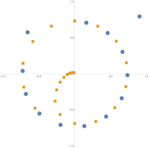
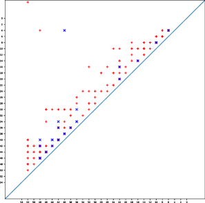
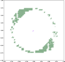
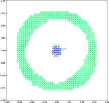
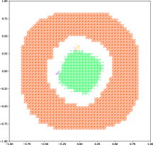
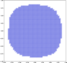
Figure 4. Upper left: two trajectories of (8) with starting points at $(-0.01,0.01)$ (squares) and $(0.9,0.8)$ (circles). Upper right: persistence diagram for a noisy sampling of (8). Red pluses and blue crosses indicate homology generators in dimension zero and one, respectively. Bottom from left to right: Morse sets in selected filtration steps for threshold values $\mu=\frac{48}{148}$ , $\mu=\frac{30}{148}$ , $\mu=\frac{6}{148}$ and $\mu=\frac{4}{148}$ , respectively.

7. Examples

In this section we present two numerical examples. The first example concerns the persistence of the Morse decompositions of a noisy sample of Kuznetsov map with respect to a frequency parameter. The second example concerns the persistence of the Morse decompositions of combinatorial multivector fields with respect to an angle parameter of the algorithm constructing the fields from a cloud of vectors.

7.1. Kuznetsov map.

Let us consider the following planar map analyzed by Kuznetsov in the context of the Neimark-Sacker bifurcation  [20, Subsection 4.6].

(8) $$N\bigg{(}\begin{bmatrix}x_{1}\\ x_{2}\end{bmatrix}\bigg{)}:=\begin{bmatrix}\cos(\theta)&-\sin(\theta)\\ \sin(\theta)&\cos(\theta)\end{bmatrix}\bigg{(}(1+\alpha)\begin{bmatrix}x_{1}\\ x_{2}\end{bmatrix}+(x_{1}^{2}+x_{2}^{2})\begin{bmatrix}a&-b\\ b&a\end{bmatrix}\begin{bmatrix}x_{1}\\ x_{2}\end{bmatrix}\bigg{)}.$$

For parameters $\theta=\pi/17$, $\alpha=0.5$, $a=-1$ and $b=0.5$ the system restricted to square $[-1,1]\times[-1,1]\subseteq\mathbb{R}^{2}$ admits a Morse decomposition consisting of an unstable fixed point and an attracting invariant circle. (see Figure 4, upper left). We want to detect this Morse decomposition just from a finite sample of the map and in the presence of Gaussian noise. The setup is similar to the toy example in Section 3.

Let $x\in\mbox{$\mathbb{R}$}^{2}$ and $\epsilon_{X},\epsilon_{Y}\in\mbox{$\mathbb{R}$}^{2}$ be random vectors chosen from normal distribution centered at zero, with standard deviation $\sigma_{X}$ and $\sigma_{Y}$ respectively. Let

(9) $$\tilde{N}(x):=N(x+\epsilon_{X})+\epsilon_{Y}$$

be a noisy version of the map (8). Consider a triangulation $K$ of the square $Q:=[-1,1]\times[-1,1]\subseteq\mathbb{R}^{2}$ obtained by splitting $Q$ into a $48\times 48$ uniform grid of squares of size $r=1/24$ and dividing every square into two triangles. Then, the set of toplexes $K_{top}$ consists of $4608$ 2-simplices. The $\sigma_{X}$, $\sigma_{Y}$ are taken to be proportional to the grid size $r$, that is $\sigma_{X}=r/4$ and $\sigma_{Y}=r$. A noisy sample $\Gamma=\{(x_{i},y_{i})\}_{i}$ of the map $N$ is generated by taking an uniformly distributed sequence of points $x_{i}$ in $Q$ and its disturbed images $y_{i}:=\tilde{N}(x_{i})$. Pairs $(x_{i},y_{i})\in\Gamma$ such that $y_{i}\not\in Q$ has been rejected from a sample. The combinatorial dynamical system $F_{\mu}$ is constructed in the same way as in Section 3, namely

(10) $$F_{\mu}(\sigma):=\operatorname{co}\bigcup_{\tau\in K_{top},\,\sigma\preceq\tau}\mbox{$\{\,\bar{\tau}\in K_{top}\mid\frac{n_{\tau,\bar{\tau}}}{n_{max}}\geq\mu\,\}$},$$

where $n_{\tau,\bar{\tau}}$ denotes the number of pairs in $\Gamma$ connecting two toplexes $\tau,\bar{\tau}\in K_{top}$, that is

(11) $$n_{\tau,\bar{\tau}}:=\#\{(x_{i},y_{i})\mid x_{i}\in\operatorname{cl}|\tau|\text{ and }y_{i}\in\operatorname{cl}|\bar{\tau}|\}$$

and $n_{max}$ is maximal of these values. For this particular experiment $n_{max}=148$. Note that construction of $F_{\mu}$ (10) is also well defined for lower dimensional simplices.

The parameter $\mu$ in (10) describes the minimal frequency of an edge to be present in the combinatorial dynamical system $F_{\mu}$. The family of Morse sets $\mathcal{M}(F_{\mu})$ at given level $\mu$ consists of all strongly connected components of an associated graph. The set of considered frequency levels $1=\mu_{74}>\mu_{73}>...>\mu_{0}=0$, where $\mu_{i}=\frac{2i}{148}$, leads to the sequence of Morse decompositions such that $\mathcal{M}(F_{\mu_{i}})\sqsubseteq\mathcal{M}(F_{\mu_{i-1}})$. The persistence diagram at Figure 4(upper right), for clarity, shows only results for $\mu\leq\mu_{27}=\frac{54}{148}$, since this is a level where Morse sets start to emerge.

Results are presented in Figure 4. As expected, the persistence diagram (Figure 4, upper right) indicates the presence of two 0-dimensional and one 1-dimensional homology generators with high persistence. Bottom row at Figure 4 shows Morse sets for selected frequency levels. For lower thresholds, both invariant sets eventually merge together creating the only strongly connected component. In the case without noise, fixed point at the origin and attracting invariant set remains separated for all values of $\mu$.

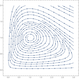
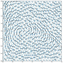
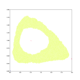
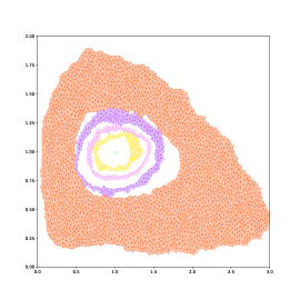
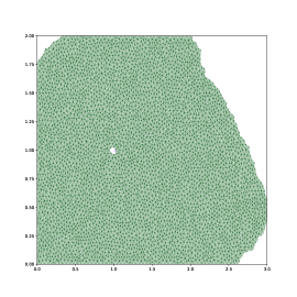
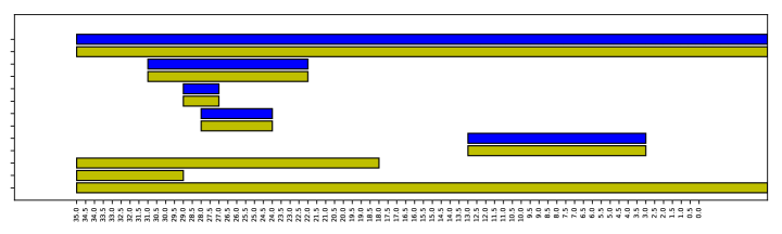
Figure 5. Top: A streamline plot and a cloud of vectors on a triangular grid for LV model. Middle from left to right: Morse decompositions of combinatorial dynamical systems constructed from the cloud for $\alpha=35^{\circ}$, $\alpha=28^{\circ}$ and $\alpha=0^{\circ}$, respectively. The mesh used contains $4756$ points and $9300$ triangles. Bottom: The respective persistence barcode. Yellow bars represents generators in dimension $0$ and blue bars in dimension $1$. The bars are ordered by average size of the Morse sets (biggest on the top).

7.2. Lotka Volterra model.

Consider the Lotka-Volterra (LV) model:

(12) $$\frac{\partial x}{\partial t}=x\left(1-\frac{x}{k}\right)-\frac{(a_{1}xy)}{b+x},\qquad\frac{\partial y}{\partial t}=\frac{a_{2}xy}{b+x}-gy,$$

where $k=3.5$, $b=1$, $g=0.5$, $a_{1}=(1-\frac{1}{k})(b+1)$, $a_{2}=g(b+1)$ (see  [6, Chapter 2, Eq. 2.13 and 2.14]). The system has a Morse decomposition consisting of a repelling stationary point and an attracting periodic orbit. We want to observe this Morse decomposition in a combinatorial dynamical system constructed from a finite sample of the vector field. In Table 1 we present an algorithm for constructing a combinatorial multivector field from a sampled vector field. The algorithm requires an angle parameter $\alpha$. The constructed combinatorial multivector field and hence its combinatorial dynamical system depend on this parameter. We execute the algorithm for varying $\alpha$ and construct the zigzag filtration (3). Since the supporting simplicial complex (mesh) remains fixed, we obtain zigzag persistence under inclusion maps. Experiments with varying mesh, utilizing non-inclusion maps, are in progress. The outcome for the LV model is presented in Figure 5. We note that the trivial Morse sets that is Morse sets consisting of just one multivector $V$ such that $H(\operatorname{cl}V,\operatorname{cl}V\setminus V)=0$ are excluded from the presentation of Morse decompositions and from the barcode, because such Morse sets are considered spurious due to the triviality of their Conley index (see [25]).

The input to the algorithm $\mathrm{CVCMF}$ in Table 1 that computes a multivector field from a cloud of vectors consists of:

• a simplicial mesh $K$ with vertices in a cloud of points $P=\{p_{i}\mid i=1,2,\ldots,n\}\subseteq\mathbb{R}^{d}$,

• the associated cloud of vectors $V:=\{\vec{v_{i}}\mid i=1,2,\ldots,n\}\subseteq\mbox{$\mathbb{R}$}^{d}$ such that vector $\vec{v_{i}}$ originates from point $p_{i}$,

• an angular parameter $\alpha$.

1:procedure CVCMF($K$, $V$, $\alpha$)

2:     $m\leftarrow$ an identity map $K\to K$.

3:     for all $\sigma\in K$ do

4:         $m[\sigma]\leftarrow$ any toplex in the star of $\sigma$ pointed by mean of $\{\,\vec{v_{i}}\in V\mid p_{i}\preceq\sigma\,\}$      

5:     for all $i=1,2,\ldots,n$ do $\triangleright$ Aligns vectors

6:         $S\leftarrow$ $\{\,(\dim\sigma,\measuredangle(\sigma,\vec{v_{i}}),\sigma)\mid\sigma\in K\text{ and }p_{i}\preceq\sigma\text{ and }\measuredangle(\sigma,\vec{v_{i}})\leq\alpha\,\}$

7:         $S^{\prime}\leftarrow$ sort $S$ using lexicographical order on first two positions $\triangleright$ $(\dim,\measuredangle,\_)$

8:         $(\_,\_,\sigma)\leftarrow$ first element of $S^{\prime}$

9:         $m[p_{i}]\leftarrow\sigma$      

10:     for all $\sigma\in K$ in descending dimension do $\triangleright$ Remove convexity conflicts

11:         while exists $\tau\preceq\sigma$ s.t. $[\tau,m[\tau]]\cap[\sigma,m[\sigma]]\neq\varnothing$ and $m[\tau]\neq m[\sigma]$ do

12:              $m[\tau]\leftarrow\sigma$ and $m[\sigma]\leftarrow\sigma$               

13:     $\text{$\mathcal{V}$}\leftarrow$ build a partition of $K$ using nonempty pre-images of $m$

14:     return $\mathcal{V}$.

Table 1. An algorithm constructing a combinatorial multivector field from a sampled vector field

For each simplex $\sigma\in K$ and a vector $\vec{v_{i}}$ originating from vertex $p_{i}$ of $\sigma$ we measure the angle between $\vec{v_{i}}$ and the affine subspaces spanned by the vertices of $\sigma$. We assume the angle to be zero when the vector has length zero or the simplex is just a vertex. For a toplex $\sigma$, we assume that the angle is zero when $\vec{v_{i}}$ points inward $\sigma$ and $\infty$ otherwise. When the angle is smaller than $\alpha$, we project $\vec{v_{i}}$ onto $\sigma$. Intuitively, it aligns the vectors to the lower dimensional simplices. After this alignment, a multivector field is constructed by removing the convexity conflicts. Obviously, the output depends on the parameter $\alpha$. We measure changes in the multivector field $\mathcal{V}$ via persistence of its Morse decomposition. To compute such persistence we use Dionysus software [24].

References

- [1] Z. Alexander, E. Bradley, J.D. Meiss, and N. Sanderson. Simplicial Multivalued Maps and the Witness Complex for Dynamical Analysis of Time Series, SIAM Journal on applied dynamical systems 14(2015), 1278–1307.
- [2] P.S. Alexandrov. Diskrete Räume, Mathematiceskii Sbornik (N.S.) 2 (1937), 501–518.
- [3] Z. Arai, W. Kalies, H. Kokubu, K. Mischaikow, H. Oka and P. Pilarczyk. A Database Schema for the Analysis of Global Dynamics of Multiparameter Systems, SIAM J. Applied Dyn. Syst. 8(2009), 757–789.
- [4] J.A. Barmak. Algebraic Topology of Finite Topological Spaces and Applications, Lecture Notes in Mathematics 2032, Springer-Verlag, 2011.
- [5] U. Bauer, H. Edelsbrunner, G. Jabłoński, M. Mrozek. Persistence in sampled dynamical systems faster, arXiv:1709.04068 (2017).
- [6] N. Boccara. Modeling Complex Systems, Springer, New York, NY 2004, ISBN 978-0-387-40462-2, https://doi.org/10.1007/b97378.
- [7] M.C. Bortolan, T. Caraballo, ,A.N. Carvalho, J.A. Langa. Skew product semiflows and Morse decomposition, J. Differential Equations 255(2013), 2436–2462.
- [8] J. Bush, M. Gameiro, S. Harker, H. Kokubu, K. Mischaikow, I. Obayashi and P. Pilarczyk. Combinatorial-topological framework for the analysis of global dynamics, Chaos 22(2012), 047508.
- [9] C. Conley. Isolated Invariant Sets and the Morse Index, American Mathematical Society, Providence, RI, 1978.
- [10] H.B. da Costa, J. Valero. Morse Decompositions with Infinite Components for Multivalued Semiflows, Set-Valued Var. Anal 25(2017), 25–41.
- [11] T. K. Dey, F. Fan, Y. Wang. Computing topological persistence for simplicial maps, Proc. 30th Annu. Sympos. Comput. Geom. (2014).
- [12] H. Edelsbrunner, G. Jabłoński, M. Mrozek. The Persistent Homology of a Self-map, Foundations of Computational Mathematics, 15(2015), 1213–1244. DOI: 10.1007/s10208-014-9223-y.
- [13] H. Edelsbrunner, D. Letscher, A. Zomorodian. Topological Persistence and Simplification, Discrete and Computational Geometry 28(2002), 511–533.
- [14] R. Forman. Morse theory for cell complexes, Advances in Mathematics, 134 (1998), 90–145.
- [15] R. Forman. Combinatorial vector fields and dynamical systems, Mathematische Zeitschrift 228 (1998), 629–681.
- [16] J. Garland, E. Bradley, J.D. Meiss. Exploring the topology of dynamical reconstructions, Physica D 334(2016), 49–59.
- [17] G. Guerrero, J.A. Langa and A. Suárez. Architecture of attractor determines dynamics on mutualistic complex networks, Nonlinear Analysis: Real World Applications 34(2017), 17–40.
- [18] D.H. Knipl, P. Pilarczyk and G.Röst. Rich Bifurcation Structure in a Two-Patch Vaccination Model, SIAM J. Applied Dynamical Systems 14(2015), 980–1017.
- [19] J. Kubica. M. Lipiński, M. Mrozek, Th. Wanner. Conley-Morse-Forman theory for generalized combinatorial multivector fields, in preparation.
- [20] Y.A. Kuznetsov. Elements of Applied Bifurcation Theory, Springer-Verlag, 1995.
- [21] M.C. McCord. Singular homology and homotopy groups of finite spaces, Duke Math. J. 33(1966), 465–474.
- [22] K. Mischaikow, M. Mrozek. Chaos in Lorenz equations: a computer assisted proof, Bull. AMS (N.S.), 33(1995), 66-72.
- [23] K. Mischaikow, M. Mrozek, J. Reiss, A. Szymczak. Construction of Symbolic Dynamics from Experimental Time Series Physical Review Letters 82(1999), p. 1144–1147.
- [24] G. Carlsson, V. de Silva, D. Morozov. Zigzag persistent homology and real-valued functions, In Proceedings of the twenty-fifth annual symposium on Computational geometry (2009), ACM, New York, NY, USA, 247-256. http://dx.doi.org/10.1145/1542362.1542408
- [25] M. Mrozek. Conley-Morse-Forman theory for combinatorial multivector fields on Lefschetz complexes, Foundations of Computational Mathematics, 17(2017), 1585–1633. DOI: 10.1007/s10208-016-9330-z.
- [26] M. Mrozek, Th. Wanner. Conley index theory for multivalued maps on finite topological spaces, in preparation.
- [27] J. Munkres. Elements of Algebraic Topology, Addison-Wesley, 1984.
- [28] J. Munkres. Topology, Prentice Hall, 1975.
- [29] J.A. Souza. On Morse decompositions of control systems, International Journal of Control, 85(2012), 815–821.
- [30] A. Szymczak. Hierarchy of Stable Morse Decompositions, IEEE Transactions on Visualization and Computer Graphics 19(2013), 799–810.
- [31] Wentao Wang, Wenke Wang, Sikun Li. From numerics to combinatorics: a survey of topological methods for vector field visualization, Journal of Visualization 19(2016) 727–752.