A Smeary Central Limit Theorem for Manifolds with Application to High Dimensional Spheres

Abstract

The (CLT) central limit theorems for generalized Fréchet means (data descriptors assuming values in stratified spaces, such as intrinsic means, geodesics, etc.) on manifolds from the literature are only valid if a certain empirical process of Hessians of the Fréchet function converges suitably, as in the proof of the prototypical BP-CLT (Bhattacharya and Patrangenaru (2005)). This is not valid in many realistic scenarios and we provide for a new very general CLT. In particular this includes scenarios where, in a suitable chart, the sample mean fluctuates asymptotically at a scale $n^{\alpha}$ with exponents $\alpha<1/2$ with a non-normal distribution. As the BP-CLT yields only fluctuations that are, rescaled with $n^{1/2}$, asymptotically normal, just as the classical CLT for random vectors, these lower rates, somewhat loosely called smeariness, had to date been observed only on the circle (Hotz and Huckemann (2015)). We make the concept of smeariness on manifolds precise, give an example for two-smeariness on spheres of arbitrary dimension, and show that smeariness, although “almost never” occurring, may have serious statistical implications on a continuum of sample scenarios nearby. In fact, this effect increases with dimension, striking in particular in high dimension low sample size scenarios.

1 Introduction

The BP-CLT

The celebrated central limit theorem (CLT) for intrinsic sample means on manifolds by Bhattacharya and Patrangenaru (2005), and many subsequent generalizations (e.g. Bhattacharya and Bhattacharya (2008); Huckemann (2011a); Bhattacharya and Patrangenaru (2013); Ellingson et al. (2013); Patrangenaru and Ellingson (2015); Bhattacharya and Lin (2017)), rests on a Taylor expansion

$$\sqrt{n}\,\mbox{\rm grad}|_{x=x_{0}}F_{n}(x)=\sqrt{n}\,\mbox{\rm grad}|_{x=0}F_{n}(x)+\mbox{\rm Hess\,}|_{x=\widetilde{x}}F_{n}(x)\sqrt{n}x_{0}$$ (1)

(with suitable $\widetilde{x}$ between $0$ and $x_{0}$) and a generalized strong law ($n\to\infty$ and $x_{0}\to 0$)

$$\mbox{\rm Hess\,}|_{x=\widetilde{x}}F_{n}(x)\operatorname{\stackrel{{\scriptstyle\mathbb{P}}}{{\to}}}\mbox{\rm Hess\,}|_{x=0}F(x)\,.$$ (2)

Here, $X_{1},\ldots,X_{n}\operatorname{\stackrel{{\scriptstyle i.i.d.}}{{\sim}}}X$ is a sample on a smooth manifold $M$,

$$F_{n}(x)=\frac{1}{n}\,\sum_{j=1}^{n}d(X_{j},\phi(x)\big{)}^{2}\,,\quad F(x)=\,\mathbb{E}[d(X,\phi(x))^{2}]$$

are the sample and population Fréchet functions with a smooth distance $d$ on $M$ and $\phi$ denotes a local smooth chart. By definition, as a minimizer of the sample Fréchet function, for the preimage $x_{0}=x_{n}$ under $\phi$ of any sample Fréchet mean, the l.h.s. of Equation (1) vanishes. If $X$ features a density near the relevant cut loci, Equation (1) is a.s. valid for deterministic points $x_{0}$ near the preimage $0$ of the population Fréchet mean, if existent (i.e. if the population Fréchet function has a unique minimizer). Further, if the empirical process on the l.h.s. of Equation (2), deterministically indexed in $\widetilde{x}$, is well defined, and not only a.s. well defined, the convergence in Equation (2) is valid also for $x_{0}=x_{n}$, and since the properly rescaled sum of i.i.d. random variables $\sqrt{n}\,\mbox{\rm grad}|_{x=0}F_{n}(x)$ converges to a Gaussian, this strain of argument gives the BP-CLT

$$\sqrt{n}x_{n}\operatorname{\stackrel{{\scriptstyle{\mathcal{D}}}}{{\to}}}{\mathcal{N}}(0,\Sigma)\,,$$ (3)

with suitable covariance matrix $\Sigma$, if the Hessian on the r.h.s of Equation (2) is invertible.

Beyond the BP-CLT

Recently in Hotz and Huckemann (2015, Example 1), an example on the circle with log coordinates $x\in[-\pi,\pi)$ has been provided, with population Fréchet mean at $x=0$ and a local density $f$ near the antipodal $-\pi$. For $x>0$ sufficiently small, the rescaled sample Fréchet function takes the value

$$nF_{n}(x) =\sum_{x-\pi\leq X_{j}}(X_{j}-x)^{2}+\sum_{X_{j}<x-\pi}(X_{j}+2\pi-x)^{2}$$

$$=\sum_{j=1}^{n}(X_{j}-x)^{2}+4\pi\sum_{X_{j}<x-\pi}(X_{j}-x+\pi)$$

so that the l.h.s. of Equation (2) is only a.s. well defined with value $\mbox{\rm Hess\,}|_{x}F_{n}(x)=2$ a.s. (as in the Euclidean case). The r.h.s., however, assume the value $\mbox{\rm Hess\,}|_{x=0}F(x)=2-4\pi f(-\pi)$. Hence, in case of $f(-\pi)\neq 0$, the convergence (2) is no longer valid, making the above strain of argument no longer viable. Still, as shown in McKilliam et al. (2012); Hotz and Huckemann (2015), as long as $2\pi f(-\pi)<1$, the BP-CLT (3) remains valid.

Further, in Hotz and Huckemann (2015) it was shown that $1=2\pi f(-\pi)$ is possible, so that the BP-CLT (3), which, under square integrability, holds universally for Euclidean spaces, is wrong for such 2D vectors confined to a circle, by giving examples in which the fluctuations may asymptotically scale with $n^{\alpha}$ with exponents $\alpha$ strictly lower than one-half.

This new phenomenon has, somewhat loosely, been called smeariness, it can only manifest in a non-Euclidean geometry. Examples beyond the circle were not known to date.

A General CLT

Making the concept of smeariness on manifolds precise, using Donsker Theory (e.g. from van der Vaart (2000)) and avoiding the sample Taylor expansion (1) as well as the non generally valid convergence condition (2), we provide for a general CLT on manifolds that requires no assumptions other than a unique population mean and a sufficiently well behaved distance. With the degree of smeariness $\kappa\geq 0$ our general CLT takes the form

$$\sqrt{n}x^{\kappa+1}_{n}\operatorname{\stackrel{{\scriptstyle{\mathcal{D}}}}{{\to}}}{\mathcal{N}}(0,\Sigma)\,,$$ (4)

where $x_{n}^{\kappa+1}$ is defined componentwise. Then, $x_{n}$ scales with $n^{\alpha}$, $\alpha={\frac{1}{2(\kappa+1)}}$, and $\kappa=0$ corresponds to the usual CLT valid on Euclidean spaces, and to the BP-CLT (3).

We phrase our general CLT in terms of sufficiently well behaved generalized Fréchet means, e.g. geodesic principal components (Huckemann and Ziezold (2006); Huckemann et al. (2010)) or principal nested spheres (Jung et al. (2012, 2011)). While we discuss some intricacies in Remark 8, their details are beyond the scope of this paper and left for future research. In general, generalized Fréchet means are random object descriptors (e.g. Marron and Alonso (2014)) that take values in a stratified space and for our general CLT we require only

1. a law of large numbers for a unique generalized Fréchet mean $\mu$,

2. a local chart at $\mu$, sufficiently smooth,

3. an a.s. Lipschitz condition and an a.s. differentiable distance between $\mu$ and data, and

4. a population Fréchet function, sufficiently smooth at $\mu$.

Further, we give an example for two-smeariness on spheres of arbitrary dimension, and show that smeariness, although “almost never” occurring, may have serious statistical implications on a continuum of sample scenarios nearby. Remarkably, this effect increases with dimension, striking in particular in high dimension low sample size scenarios.

2 A General Central Limit Theorem

In a typical scenario of non-Euclidean statistics, a two-sample test is applied to two groups of manifold-valued data or more generally to data on a manifold-stratified space. Such a test can be based on certain data descriptors such as intrinsic means (e.g. Bhattacharya and Patrangenaru (2005); Munk et al. (2008); Patrangenaru and Ellingson (2015)), best approximating geodesics (e.g. Huckemann (2011b)), best approximating subspaces within a given family of subspaces and entire flags thereof (cf. Huckemann and Eltzner (2017)), and asymptotic confidence regions can be constructed from a suitable CLT for such descriptors. In this section we first introduce the setting of generalized Fréchet means along with standard assumptions, we then recollect and expand some Donsker Theory from van der Vaart (2000) and state and prove our general CLT.

2.1 Generalized Fréchet Means and Assumptions

Fréchet functions and Fréchet means have been first introduced by Fréchet (1948) for squared metrics $\widetilde{\rho}:Q\times Q\to[0,\infty)$ on a topological space $Q$ and later extended to squared quasimetrics by Ziezold (1977). Generalized Fréchet means as follows have been introduced by Huckemann (2011b). A simple setting is given when $P=Q$ is a Riemannian manifold and $\widetilde{\rho}=d^{2}$ is the squared geodesic intrinsic distance. Then a generalized Fréchet mean is a minimizer with respect to squared distance, often called a barycenter.

Notation 1.

Let $P$ and $Q$ be separable topological spaces, $Q$ is called the data space and $P$ is called the descriptor space, linked by a continuous map $\widetilde{\rho}:P\times Q\to[0,\infty)$ reflecting distance between a data descriptor $p\in P$ and a datum $q\in Q$. Further, with a silently underlying probability space $(\Omega,\mathfrak{A},\mathbb{P})$, let $X_{1},\ldots,X_{n}\operatorname{\stackrel{{\scriptstyle i.i.d.}}{{\sim}}}X$ be random elements on $Q$, i.e. they are Borel-measurable mappings $\Omega\to Q$. They give rise to generalized population and generalized sample Fréchet functions,

$$\widetilde{F} :p\mapsto\mathbb{E}[\widetilde{\rho}(p,X)]\,, \widetilde{F}_{n} :p\mapsto\frac{1}{n}\sum_{j=1}^{n}\limits\widetilde{\rho}(p,X_{j})]\,,$$

respectively, and their generalized population and generalized sample Fréchet means

$$\widetilde{E} =\left\{p\in P:\widetilde{F}(p)=\inf_{p\in P}\limits\widetilde{F}(p)\right\}\,, \widetilde{E}_{n} =\left\{p\in P:\widetilde{F}_{n}(p)=\inf_{p\in P}\limits\widetilde{F}_{n}(p)\right\}\,,$$

respectively. Here the former set is empty if the expected value is never finite.

With Assumption 2.3 further down, $P$ is a manifold locally near $\mu$, so that convergence in probability in the following assumption is well defined.

Assumption 2 (Unique Mean with Law of Large Numbers).

In fact, we assume that $\widetilde{E}$ is not empty but contains a single descriptor $\mu\in P$ and that for every measurable selection $\mu_{n}\in\widetilde{E}$,

$$\mu_{n}\operatorname{\stackrel{{\scriptstyle\mathbb{P}}}{{\to}}}\mu\,.$$

Assumption 3 (Local Manifold Structure).

With $2\leq r\in\mathbb{N}$ assume that there is a neighborhood $\widetilde{U}$ of $\mu$ that is an $m$-dimensional Riemannian manifold, $m\in\mathbb{N}$, such that with a neighborhood $U$ of the origin in $\mathbb{R}^{m}$ the exponential map $\exp_{\mu}:U\to\widetilde{U}$, $\exp_{\mu}(0)=\mu$, is a $C^{r}$-diffeomorphism, and we set for $p=\exp_{\mu}(x),p^{\prime}=\exp_{\mu}(x^{\prime})\in\widetilde{U}$ and $q\in Q$,

$$\rho :(x,q)\mapsto\widetilde{\rho}(\exp_{\mu}(x),q)\,,$$

$$F :x\mapsto\widetilde{F}(\exp_{\mu}(x))\,, F_{n} :x\mapsto\widetilde{F}_{n}(\exp_{\mu}(x))\,.$$

It will be convenient to extend $F_{n}$ to all of $\mathbb{R}^{m}$ via $F_{n}(x)=F_{n}(0)$ for $x\in\mathbb{R}^{m}\setminus U$.

Assumption 4 (Almost Surely Locally Lipschitz and Differentiable at Mean).

Further assume that

1. the gradient $\dot{\rho}_{0}(X):=\mbox{\rm grad}_{x}\rho(x,X)|_{x=0}$ exists almost surely;

2. there is a measurable function $\dot{\rho}:Q\to\mathbb{R}$ satisfying $\mathbb{E}[\dot{\rho}(X)^{2}]<\infty$ for all $x\in U$ and that the following Lipschitz condition

   $$|\rho(x_{1},X)-\rho(x_{2},X)|\leq\dot{\rho}(X)\|x_{1}-x_{2}\|\mbox{\rm~{}a.s.}$$

   holds for all $x_{1},x_{2}\in U$.

Assumption 5 (Smooth Fréchet Function).

With $2\leq r\in\mathbb{N}$ and a non-vanishing tensor $T=(T_{j_{1},\ldots,j_{r}})_{1\leq j_{1}\leq\ldots\leq j_{r}\leq m}$, assume that the Fréchet function admits the power series expansion

$$F(x) =F(0)+\sum_{1\leq j_{1}\leq\ldots\leq j_{r}\leq m}x_{j_{1}}\ldots x_{j_{r}}T_{j_{1},\ldots,j_{r}}+o(\|x\|^{r})\,.$$ (5)

The tensor in $T$ in (5) can be very complicated. As is well known, for $r=2$, every symmetric tensor is diagonalizable ($m(m+1)/2$ parameters involved), which is, however, not true in general. For simplicity of argument, however, we assume that $T$ is diagonalizable with non-zero diagonal elements so that Assumption 5 rewrites as follows. In this formulation, we can also drop our assumption that $r\in\mathbb{N}$.

Assumption 6.

With $2\leq r\in\mathbb{R}$, a rotation matrix $R\in SO(m)$ and $T_{1},\ldots,T_{m}\neq 0$ assume that the Fréchet function admits the power series expansion

$$F(x) =F(0)+\sum_{j=1}^{m}\limits T_{j}|(Rx)_{j}|^{r}+o(\|x\|^{r})\,.$$ (6)

Remark 7 (Typical Scenarios).

Let us briefly recall typical scenarios. In many applications, $Q$ is

1. globally a complete smooth Riemannian manifold, e.g. a sphere (cf. Mardia and Jupp (2000) for directional data), a real or complex projective space (cf. Kendall (1984); Mardia and Patrangenaru (2005) for certain shape spaces) or the space of positive definite matrices (cf. Dryden et al. (2009) for diffusion tensors),

2. a non-manifold shape space which is a quotient of a Riemannian manifold under an isometric group action with varying dimensions of isotropy groups (e.g..Dryden and Mardia (1998); Kendall et al. (1999), for spaces of three- and higher-dimensional shapes),

3. a general stratified space where all strata are manifolds with compatible Riemannian structures, e.g. phylogenetic tree spaces (cf. Billera et al. (2001); Moulton and Steel (2004), for varying geometries).

On these spaces,

• in most of the above applications, $P=Q$ and intrinsic means are considered where $\widetilde{\rho}$ is the squared geodesic distance induced from the Riemannian structure.

• In other examples, $P=\Gamma$, the space of geodesics on $Q$ is considered, in view of PCA-like dimension reduction methods (e.g. Fletcher and Joshi (2004); Huckemann and Ziezold (2006); Huckemann et al. (2010)), or

• $P$ is a family of subspaces of $Q$, or even a space of nested subspheres in Jung et al. (2012, 2011); more general families have been recently considered in generic dimension reduction methods, e.g. Sommer (2016); Pennec (2017).

Remark 8.

Of the above assumptions some are harder to prove in real examples than others.

1. Of all above assumptions, uniqueness (first part of Assumption 2) seems most challenging to verify. To date, only for intrinsic means on the circle the entire picture is known, cf. Hotz and Huckemann (2015, p. 182 ff.). For complete Riemannian manifolds, uniqueness for intrinsic means has been shown if the support is sufficiently concentrated (cf. Karcher (1977); Kendall (1990); Le (2001); Groisser (2005); Afsari (2011)) and intrinsic sample means are unique a.s. if from a distribution absolutely continous w.r.t. Riemannian measure, cf. Bhattacharya and Patrangenaru (2003, Remark 2.6) (for the circle) and Arnaudon and Miclo (2014, Theorem 2.1) (in general).

2. For the above typical scenarios, we anticipate that the other assumptions are often valid in concrete applications.

   For instance, Assumption 3 is also true on non-manifold shape spaces, due to the manifold stability theorem Huckemann (2012, Corollary 1). It may be not be valid, however, on arbitrary stratified spaces, cf. Hotz et al. (2013); Huckemann et al. (2015).

3. Moreover, Assumption 4 is only slightly stronger than uniform coercivity (condition (2) in Huckemann (2011b, p. 1118)) which suffices for the strong law (second part of Assumption 2), cf. Huckemann (2011b, Theorem A4) and Huckemann and Eltzner (2017, Theorem 4.1), and this has been established for principal nested spheres in Huckemann and Eltzner (2017, Theorem 3.8) and for geodesics with nested mean on Kendall’s shape spaces in Huckemann and Eltzner (2017, Theorem 3.9). In consequence of Lemma 20 below, we have that Assumption 4 holds for intrinsic means of distributions on spheres which feature a density near the antipodal of the intrinsic population mean.

A more detailed analysis is beyond the scope of this paper and left for future research.

2.2 General CLT

For the following, fix a measurable selection $\mu_{n}\in\widetilde{E}_{n}$. Due to $\mu_{n}\operatorname{\stackrel{{\scriptstyle\mathbb{P}}}{{\to}}}\mu$ from Assumption 2, we have $\mathbb{P}\{\mu_{n}\in\widetilde{U}\}\to 1$, and in accordance with the convention in Assumption 3, setting

$$x_{n}:=\left\{\begin{array}[]{cl}\exp^{-1}_{\mu}(\mu_{n})&\mbox{ if }\mu_{n}\in\widetilde{U}\\ 0&\mbox{ else}\end{array}\right.\,,$$

note that

$$F_{n}(0)\geq F_{n}(x_{n})=\widetilde{F}_{n}(\mu_{n})+o_{p}(1)\,,$$ (7)

because $\mathbb{P}\{F_{n}(x_{n})-\widetilde{F}_{n}(\mu_{n})>\epsilon\}=\mathbb{P}\{\mu_{n}\not\in\widetilde{U}\}\to 0$ for all $\epsilon>0$.

The following is a direct consequence of van der Vaart (2000, Lemma 5.52), replacing maxima with minima, where, due to continuity of $\widetilde{\rho}$, we have no need for outer measure and outer expectation, and, due to our setup, no need for approximate minimizers.

Lemma 9.

Assume that for fixed constants $C$ and $\alpha>\beta$ for every $n$ and for sufficiently small $\delta$

$$\sup_{\|x\|<\delta}\limits\left|F(x)-F(0)\right| \leq C\delta^{\alpha}\,,$$ (8)

$$\mathbb{E}\left[n^{1/2}\sup_{\|x\|<\delta}\limits\big{|}F_{n}(x)-F(x)-F_{n}(0)+F(0)\big{|}\right] \leq C\delta^{\beta}\,.$$ (9)

Then, any a random sequence $\mathbb{R}^{m}\ni y_{n}\operatorname{\stackrel{{\scriptstyle\mathbb{P}}}{{\to}}}0$ that satisfies $F_{n}(y_{n})\leq F_{n}(0)$ also satisfies $n^{1/(2\alpha-2\beta)}y_{n}=\mathcal{O}_{P}(1)$.

As a first step, the following generalization of van der Vaart (2000, Corollary 5.53, only treating the case $r=2$) gives a bound for the scaling rate in the general CLT, so that also in case of $r\geq 2$, $\sqrt{n}x_{n}=o_{p}(1)$.

Corollary 10.

Under Assumptions 2, 3 and 4, as well as Assumption 5 or 6,

$$n^{1/(2r-2)}x_{n}=\mathcal{O}_{P}(1)\,.$$

Proof.

By Assumption 2 and definition, $x_{n}\operatorname{\stackrel{{\scriptstyle\mathbb{P}}}{{\to}}}0$ with $F_{n}(x_{n})\leq F_{n}(0)$, cf. (7). Hence, Lemma 9 yields the assertion, because for $\alpha=r$, (8) follows at once from (5) or from (6), and under Assumption 4, (9), for $\beta=1$ follows word by word from the proof of van der Vaart (2000, Corollary 5.53). ∎

As the second step, the following Theorem, which is a generalization and adaption of van der Vaart (2000, Theorem 5.23), shows that under Assumption 6 the above bound gives the exact scaling rate, including the explicit limiting distribution.

Theorem 11 (General CLT for Generalized Fréchet Means).

Under Assumptions 2, 3, 4 and 6, we have

$$n^{1/2}\left((Rx_{n})_{1}|(Rx_{n})_{1}|^{r-2},\ldots,(Rx_{n})_{m}|(Rx_{n})_{m}|^{r-2}\right)^{T}$$

$$\operatorname{\stackrel{{\scriptstyle{\mathcal{D}}}}{{\to}}}\quad {\mathcal{N}}\left(0,\frac{1}{r^{2}}T^{-1}\mbox{\rm Cov}[\mbox{\rm grad}|_{x=0}\rho(x,X)]T^{-1}\right)\,$$

with $T=\mbox{\rm diag}(T_{1},\ldots,T_{m})$. In particular for every coordinate $j=1,\ldots,m$,

$$n^{\frac{1}{2r-2}}(R^{T}x_{n})_{j}\operatorname{\stackrel{{\scriptstyle{\mathcal{D}}}}{{\to}}}{\cal H}_{j}$$

where $(\operatorname{sign}({\cal H}_{1}){\cal H}_{1}^{r-1},\ldots,\operatorname{sign}({\cal H}_{1}){\cal H}_{m}^{r-1})$ has the above multivariate Gaussian limiting distribution.

Proof.

For $z\in U$ and $2(r-1)=1/s$, let us abbreviate

$$\tau_{n}(z,X) :=n^{s}(\rho(zn^{-s},X)-\rho(0,X))-z^{T}\dot{\rho}_{0}(X)$$

$$G_{n} :=n^{1/2}\left(\frac{1}{n}\sum_{j=1}^{n}\dot{\rho}_{0}(X_{j})-\mathbb{E}\left[\dot{\rho}_{0}(X)\right]\right)\,,$$

where we set $\rho(zn^{-s},X)=\rho(0,X)$ if $zn^{-s}\not\in U$. Then, due to Assumptions 4 and 6, and $1/2+s-sr=0$,

$$n^{1/2}\left(\frac{1}{n}\sum_{j=1}^{n}\limits\left(\tau_{n}(z,X_{j})\right)-\mathbb{E}\left[\tau_{n}(z,X)\right]\right)$$

$$= n^{1/2+s}\Big{(}F_{n}(zn^{-s})-F_{n}(0)-F(zn^{-s})+F(0)\Big{)}-z^{T}G_{n}$$

$$= n^{1/2+s}\Big{(}F_{n}(zn^{-s})-F_{n}(0)\Big{)}-\sum_{j=1}^{m}\limits T_{j}|(Rz)_{j}|^{r}-z^{T}G_{n}+o(\|z\|^{r})$$

is a sequence of stochastic processes, indexed in $z\in U$, with zero expectation and variance converging to zero. By argument from the proof of van der Vaart (2000, Lemma 19.31), due to Assumption 4, $z$ can be replaced with any random sequence $z_{n}=O_{p}(1)$, cf. also the proof of van der Vaart (2000, Lemma 5.23) for $r=2$, yielding,

$$n^{1/2+s}\Big{(}F_{n}(z_{n}n^{-s})-F_{n}(0)\Big{)}=\sum_{j=1}^{m}\limits T_{j}|(Rz_{n})_{j}|^{r}+z_{n}^{T}G_{n}+o_{P}(1)\,.$$ (10)

By Corollary 10, $z_{n}=x_{n}n^{s}$ is a valid choice in equation (10). Comparison with any other $z_{n}=O_{P}(1)$, because $\mu_{n}$ is a minimizer for $\widetilde{F}_{n}$ and $F_{n}(x_{n})$ deviates only up to $o_{p}(1)$ from $\widetilde{F}_{n}(\mu_{n})$, due to (7), reveals,

$$n^{1/2+s}\Big{(}F_{n}(x_{n})-F_{n}(0)\Big{)}\leq n^{1/2+s}\Big{(}F_{n}(z_{n}n^{-s})-F_{n}(0)\Big{)}+o_{P}(1)\,.$$

This asserts that $Rx_{n}n^{s}$ is a minimizer, up to $o_{P}(1)$, of the right hand side of (10), i.e. of

$$f:w \mapsto f(w):=\sum_{j=1}^{m}\limits T_{j}|(w)_{j}|^{r}+w^{T}RG_{n}\,.$$

This function, however, has a unique minimizer, given on the component level ($j=1,\ldots,m$) by

$$rT_{j}\operatorname{sign}((w_{n})_{j})|(w_{n})_{j}|^{r-1}=-(RG_{n})_{j}\quad\mbox{ i.e. }\quad(w_{n})_{j}|(w_{n})_{j}|^{r-2}=-\frac{(RG_{n})_{j}}{rT_{j}}\,,$$

yielding

$$\sqrt{n}(Rx_{n})_{j}|(Rx_{n})_{j}|^{r-2} =-\frac{(RG_{n})_{j}}{rT_{j}}+o_{P}(1)\,.$$

Now the classical CLT gives the first assertion. The second also follows from the above display, since for $z=(Rx_{n})_{j}$ and $H=-(RG_{n})_{j}/rT_{j}$, the equation $\sqrt{n}\operatorname{sign}(z)|z|^{r-1}=H$ implies $\operatorname{sign}(z)=\operatorname{sign}(H)$ and hence

$$n^{\frac{1}{2r-2}}z=n^{\frac{1}{2r-2}}\operatorname{sign}(z)|z|=\operatorname{sign}(H)|H|^{\frac{1}{r-1}}\,.$$

∎

Remark 12.

The above arguments rely among others on the fact that due to Assumption 4, a specific convergence, different from (2), that can be easily verified for empirical processes indexed in a deterministic bounded variable, are also valid if the index varies randomly, bounded in probability. This can be weakened to the requirement, that the function class $\rho(x,\cdot)$ possesses the Donsker property, cf. van der Vaart (2000, Chapter 19).

3 Smeariness

Recall from Huckemann (2015) that a sequence of random vectors $X_{n}$ is $k$-th order smeary if $n^{\frac{1}{2(k+1)}}X_{n}$ has a non-trivial limiting distribution as $n\to\infty$.

With this notion, the classical central limit theorem in particular asserts for random vectors with existing second moments that the fluctuation of sample means around the population mean is $0$-th order smeary, also called nonsmeary.

It has been shown in Hotz and Huckemann (2015) that the fluctuation of random directions on the circle of sample means around the population mean may feature smeariness of any given positive integer order. It has been unknown to date, however, whether the phenomenon of smeariness extends to higher dimensions, in particular, to positive curvature.

To this end, we now make the concept of smeariness on manifolds precise.

Definition 13.

Let $(\Omega,\mathfrak{A},\mathbb{P})$ be a probability space, $X:\Omega\to\mathbb{R}^{m}$ a non-deterministic random vector and $k>-1$. Then a sequence of Borel measurable mappings $X_{n}:\Omega_{n}\to\mathbb{R}^{m}$ ($n\in\mathbb{N}$) with $\Omega_{n}\in\mathfrak{A}$, $\mathbb{P}(\Omega_{n})\to 1$ ($n\to\infty$) is $k$-smeary with limiting distribution of $X$ if

$$\mathbb{P}\left\{n^{\frac{1}{2(k+1)}}X_{n}\in B|\Omega_{n}\right\} \to\mathbb{P}\{X\in B\}\mbox{ as }n\to\infty\mbox{ for all Borel sets }B\subset\mathbb{R}^{m}\,.$$

In this case we write $n^{\frac{1}{2(k+1)}}X_{n}\operatorname{\stackrel{{\scriptstyle{\mathcal{D}}}}{{\to}}}X$.

Note that $-1<k$-smeariness implies that $\mathbb{P}\{X_{n}\in B|\Omega_{n}\}\to 1_{0\in B}$ for all Borel $B\subset\mathbb{R}^{m}$. As usual, we abbreviate this with $X_{n}\operatorname{\stackrel{{\scriptstyle\mathbb{P}}}{{\to}}}0$.

Lemma 14.

Let $X_{n}:\Omega_{n}\to\mathbb{R}^{m}$ be Borel measurable with $\mathbb{P}(\Omega_{n})\to 1$ and $X_{n}\operatorname{\stackrel{{\scriptstyle\mathbb{P}}}{{\to}}}0$, consider a continuously differentiable local bijection $\Phi:U\to V$ preserving the origin $0\in U,V$ open $\subset\mathbb{R}^{m}$, set $Y_{n}=\Phi(X_{n}):\Omega_{n}\cap\{X_{n}\in U\}\to\mathbb{R}^{m}$ and let $k>-1$. Then

$X_{n}$ is $k$-smeary $\Leftrightarrow$ $Y_{n}$ is $k$-smeary.

In particular, if $X$ has the limiting distribution of $n^{\frac{1}{2(k+1)}}X_{n}$, then $D\Phi(0)X$ has the limiting distribution of $n^{\frac{1}{2(k+1)}}Y_{n}$. Here $D\Phi(x)$ denotes the differential of $\Phi$ at $x\in U$ and $\det\big{(}D\Phi(0)\big{)}\neq 0$ due to invertibility of $\Phi$.

Proof.

The implication “$\Rightarrow$” is a direct consequence of a Taylor expansion and the continuity theorem with a suitable point $\widetilde{X}_{n}\operatorname{\stackrel{{\scriptstyle\mathbb{P}}}{{\to}}}0$ between the origin and $X_{n}$ as follows

$$\mathbb{P}\left\{n^{\frac{1}{2(k+1)}}Y_{n}\in B|\Omega_{n}\cap\{X_{n}\in U\}\right\} =\mathbb{P}\left\{n^{\frac{1}{2(k+1)}}D\Phi(\widetilde{X}_{n})X_{n}\in B|\Omega_{n}\cap\{X_{n}\in U\}\right\}$$

$$\to\mathbb{P}\left\{D\Phi(0)X\in B\right\}$$

because $\mathbb{P}\{X_{n}\in U\}\to 1$ due to $X_{n}\operatorname{\stackrel{{\scriptstyle\mathbb{P}}}{{\to}}}0$.

Similarly, the implication “$\Leftarrow$” follows. Suppose that $Y$ has the limiting distribution of $n^{\frac{1}{2(k+1)}}Y_{n}$. Then

$$\mathbb{P}\left\{n^{\frac{1}{2(k+1)}}X_{n}\in B|\Omega_{n}\right\} =\mathbb{P}\left\{n^{\frac{1}{2(k+1)}}D\Phi(\widetilde{X}_{n})^{-1}Y_{n}\in B|\Omega_{n}\cap\{X_{n}\in U\}\right\}$$

$$\hskip 56.9055pt+\mathbb{P}\left\{n^{\frac{1}{2(k+1)}}X_{n}\in B|\Omega_{n}\cap\{X_{n}\not\in U\}\right\}$$

$$\to\mathbb{P}\left\{D\Phi(0)^{-1}Y\in B\right\}\,,$$

again due to the hypothesis $X_{n}\operatorname{\stackrel{{\scriptstyle\mathbb{P}}}{{\to}}}0$. ∎

In consequence of Lemma 14, we have the following general definition.

Definition 15.

A sequence $\mu_{n}\operatorname{\stackrel{{\scriptstyle\mathbb{P}}}{{\to}}}\mu$ of random variables on a $m$-dimensional manifold $M$ is $k$-smeary if in one – and hence in every – continuously differentiable chart $\phi^{-1}:\widetilde{U}\to\mathbb{R}^{m}$ around $\mu\in\widetilde{U}\subset M$ the sequence of vectors $\phi^{-1}(\mu_{n})-\phi^{-1}(\mu):\{\mu_{n}\in\widetilde{U}\}\to\mathbb{R}^{m}$ is $k$-smeary.

Remark 16.

In particular, the order of smeariness is independent of the chart chosen.

4 An Example of Two-Smeariness on Spheres

4.1 Setup

Consider a random variable $X$ distributed on the $m$-dimensional unit sphere ${{\mathbb{S}}^{m}}$ ($m\geq 2$) that is uniformly distributed on the lower half sphere ${\mathbb{L}}^{m}=\{q\in{{\mathbb{S}}^{m}}:q_{2}\leq 0\}$ with total mass $0<\alpha<1$ and assuming the north pole $\mu=(0,1,0,\ldots,0)^{T}$ with probability $1-\alpha$. Then we have the Fréchet function

$$\widetilde{F}:{{\mathbb{S}}^{m}}\to[0,\infty),~{}p\mapsto\int_{{\mathbb{S}}^{m}}\widetilde{\rho}(p,q)\,d\mathbb{P}^{X}(q)$$

involving the squared spherical distance $\widetilde{\rho}(p,q)=\arccos\langle p,q\rangle^{2}$ based on the standard inner product $\langle\cdot,\cdot\rangle$ of $\mathbb{R}^{m+1}$. Every minimizer $p^{*}\in{{\mathbb{S}}^{m}}$ of $F$ is called an intrinsic Fréchet population mean of $X$.

With the volume of ${{\mathbb{S}}^{m}}$ given by

$$v_{m}={\mbox{\rm vol}}({{\mathbb{S}}^{m}})=\frac{2\pi^{\frac{m+1}{2}}}{\Gamma\left(\frac{m+1}{2}\right)}$$

define

$$\gamma_{m}=\frac{v_{m+1}}{2v_{m}}=\frac{\sqrt{\pi}}{2}\,\frac{\Gamma\left(\frac{m+1}{2}\right)}{\Gamma\left(\frac{m+2}{2}\right)}\,.$$

Moreover, we have the exponential chart centered at $\mu\in{{\mathbb{S}}^{m}}$ with inverse

$$\exp_{\mu}^{-1}(p)=(e_{1},e_{3},\ldots,e_{m+1})^{T}\big{(}p-\langle p,\mu\rangle\mu\big{)}\frac{\arccos\langle p,\mu\rangle}{\|p-\langle p,\mu\rangle\mu\|}=x\in\mathbb{R}^{m}\,$$

where $e_{1},\ldots,e_{m+1}$ are the standard unit column vectors in $\mathbb{R}^{m+1}$. Note that $\exp_{\mu}^{-1}$ has continuous derivatives of any order in $\widetilde{U}={{\mathbb{S}}^{m}}\setminus\{-\mu\}$ and recall that $e_{2}=\mu$.

4.2 Derivatives of the Fréchet Function

Lemma 17.

With the above notation, the function $F=\widetilde{F}\circ\exp_{\mu}$ has derivatives of any order for $x\in\exp_{\mu}^{-1}(\widetilde{U})$ with $\|x\|<\pi/2$. For $\alpha=1/(1+\gamma_{m})$ the north pole $\mu$ gives the unique intrinsic Fréchet mean with $\mbox{\rm Hess\,}|_{x=0}F\circ\exp_{\mu}(x)=0$. Moreover, for any choice of $0<\alpha<1$,

$$\partial_{i}\partial_{k}\partial_{l}|_{x=0}F =0$$

$$\partial_{i}\partial_{k}\partial_{l}\partial_{s}|_{x=0}F =c_{m}\delta_{i,k,l,s}$$

for every $1\leq i,k,l,s\leq m$ with the constant $c_{m}=\frac{2\gamma_{m}}{1+\gamma_{m}}\,\frac{m-1}{m+2}>0$.

Proof.

For convenience we choose polar coordinates $\theta_{1},\ldots,\theta_{m-1}\in[-\pi/2,\pi/2]$ and $\phi\in[-\pi,\pi)$ in the non-standard way

$$q=\begin{pmatrix}q_{1}\\ q_{2}\\ \vdots\\ q_{m-1}\\ q_{m}\\ q_{m+1}\end{pmatrix}=\begin{pmatrix}-\left(\prod_{j=1}^{m-1}\cos\theta_{j}\right)\cos\phi\\ -\left(\prod_{j=1}^{m-1}\cos\theta_{j}\right)\sin\phi\\ \vdots\\ -\cos\theta_{1}\,\cos\theta_{2}\,\sin\theta_{3}\\ -\cos\theta_{1}\,\sin\theta_{2}\ \\ \sin\theta_{1}\end{pmatrix}\,,$$

such that the north pole $\mu$ has coordinates $(0,\ldots,0,-\pi/2)$. In fact, we have chosen these coordinates so that w.l.o.g. we may assume that the arbitrary but fixed point $p\in{{\mathbb{S}}^{m}}$ has coordinates $(0,0,\ldots,0,-\pi/2+\delta)$ with suitable $\delta\in[0,\pi]$. Setting $\Theta=[-\pi/2,\pi/2]$, with the function

$$g:\Theta^{m-1}\to[0,1],~{}\theta=(\theta_{1},\ldots,\theta_{m-1})\mapsto\prod_{j=1}^{m-1}\cos^{m-j}\theta_{j}$$

we have the spherical volume element $g(\theta)\,d\theta\,d\phi$. Additionally defining

$$h(\theta)=\prod_{j=1}^{m-1}\cos\theta_{j}\,,$$

we have that

$$\widetilde{F}(p) =\widetilde{F}(\mu)+\frac{2\alpha}{v_{m}}\big{(}C_{+}(\delta)-C_{-}(\delta)\big{)}+\delta^{2}(1-\alpha)=:G(\delta)$$

with the two “crescent” integrals

$$C_{+}(\delta) =\int_{\Theta^{m-1}}\limits d\theta\,g(\theta)\,\int_{-\delta}^{0}\limits d\phi\,\widetilde{\rho}(\mu,q)^{2}=\int_{\Theta^{m-1}}\limits d\theta\,g(\theta)\,\int^{\delta}_{0}\limits\Big{(}\arccos\big{(}h(\theta)\,\sin\phi)\big{)}\Big{)}^{2}\,d\phi$$

$$C_{-}(\delta) =\int_{\Theta^{m-1}}\limits d\theta\,g(\theta)\,\int_{\pi-\delta}^{\pi}\limits d\phi\,\widetilde{\rho}(\mu,q)^{2}=\int_{\Theta^{m-1}}\limits d\theta\,g(\theta)\,\int_{0}^{\delta}\limits\Big{(}\arccos\big{(}-h(\theta)\,\sin\phi)\big{)}\Big{)}^{2}\,d\phi$$

cf. Figure 1, because the spherical measure of ${\mathbb{L}}^{m}$ is $v_{m}/2$.

Since for $a\in[0,1]$,

$$\big{(}\arccos(a\big{)})^{2}-\big{(}\arccos(-a)\big{)}^{2} =\big{(}\arccos(a)+\arccos(-a)\big{)}\big{(}\arccos(a)-\arccos(-a)\big{)}$$

$$=2\pi\left(\frac{\pi}{2}-\arccos(a)\right)=-2\pi\arcsin(a)\,,$$

which has arbitrary derivatives if $-1<a<1$, we have that

$$\widetilde{F}\circ\exp_{\mu}(x)=G(\delta)=G(0)-\frac{4\pi\alpha}{v_{m}}\int_{\Theta^{m-1}}\limits d\theta\,g(\theta)\,\int^{\delta}_{0}\limits\arcsin\big{(}h(\theta)\,\sin\phi\big{)}\,d\phi+\delta^{2}(1-\alpha)$$ (11)

for every $x\in\exp_{\mu}^{-1}(\widetilde{U})$ with $\|x\|=\delta$, yielding the first assertion of the Lemma.

For the second assertion we use the Taylor expansion

$$\arcsin\big{(}h(\theta)\,\sin\phi\big{)}=\phi\,h(\theta)+\frac{\phi^{3}}{6}\big{(}h(\theta)^{3})-h(\theta)\big{)}+O(\phi^{5})$$ (12)

and compute for $k=0,1,\ldots$,

$$\int_{\Theta^{m-1}}\limits g(\theta)\,h(\theta)^{k}\,d\theta =\int_{\Theta^{m-1}}\prod_{j=1}^{m-1}\left(\cos^{m-j+k}\theta_{j}\,d\theta_{j}\right)$$

$$=\int_{\Theta^{m+k-1}}\prod_{j=1}^{m+k-1}\left(\cos^{m+k-j}\theta_{j}\,d\theta_{j}\right)\Big{/}\int_{\Theta^{k}}\prod_{j=1}^{k}\left(\cos^{j}\theta_{j}\,d\theta_{j}\right)$$

$$=\frac{v_{m+k}}{v_{k+1}}\,,$$ (13)

to obtain, in conjunction with (11),

$$G(\delta) =G(0)+\delta^{2}\left(1-\alpha\left(1+\frac{v_{m+1}}{2v_{m}}\right)\right)+\frac{\delta^{4}}{24}\,\frac{\alpha v_{m+1}}{v_{m}}\,\frac{m-1}{m+2}+\ldots$$

which yields that for any choice of $\alpha\in[0,1]$ we have $G^{\prime}(0)=0=G^{\prime\prime\prime}(0)$, as well as $G^{\prime\prime}(0)\geq 0$ for $1\geq\alpha\left(1+\gamma_{m}\right)$ with equality for $\alpha=1/\left(1+\gamma_{m}\right)$. Since $G^{\prime\prime\prime\prime}(0)=\frac{\alpha v_{m+1}}{v_{m}}\,\frac{m-1}{m+2}=c_{m}>0$ for all $\alpha\in(0,1)$, this guarantees a local minimum for $\alpha=1/(1+\gamma_{m})$.

In order to see that $\mu$ gives the global minimum in case of $\alpha=1/\left(1+\frac{v_{m+1}}{2v_{m}}\right)$ we consider the derivatives

$$G^{\prime}(\delta) =-\frac{4\pi\alpha}{v_{m}}\int_{\Theta^{m-1}}\limits g(\theta)\,\arcsin\big{(}h(\theta)\,\sin\delta\big{)}\,d\theta+2\delta(1-\alpha)\,,$$

$$G^{\prime\prime}(\delta) =-\frac{4\pi\alpha}{v_{m}}\int_{\Theta^{m-1}}\limits g(\theta)\,h(\theta)\,\frac{\cos\delta}{\sqrt{1-h(\theta)^{2}\,\sin^{2}\delta}}\,d\theta+2(1-\alpha)$$ (14)

$$\geq-\frac{4\pi\alpha}{v_{m}}\int_{\Theta^{m-1}}\limits g(\theta)\,h(\theta)\,d\theta+2(1-\alpha)=2-\alpha\left(2+\frac{v_{m+1}}{v_{m}}\right)=0\,,$$

where the inequality is strict for $\delta\neq 0,\pi$, i.e. $p\neq\pm\mu$, due to $0<h(\theta)<1$ for all $\theta\in(-\pi/2,\pi/2)^{m-1}$. Hence we infer that $G^{\prime}(\delta)$ is strictly increasing in $\delta$ from $G^{\prime}(0)=0$, yielding that there is no stationary point for $F$ other than $p=\mu$.

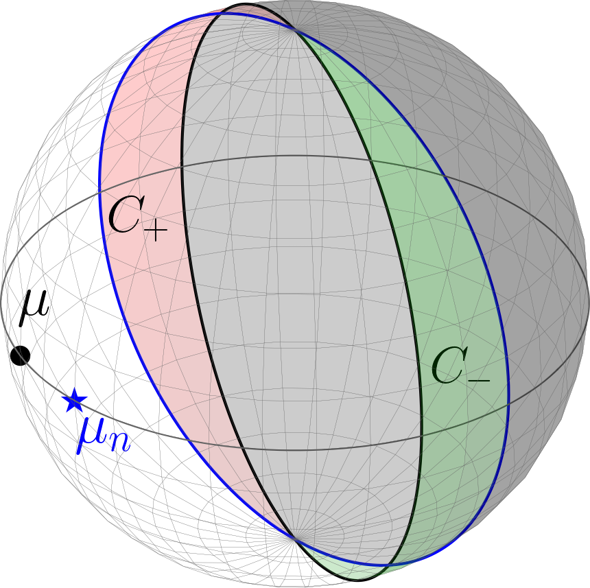
Figure 1: Depicting the two crescents $C_{+}=C_{+}(\delta)$ and $C_{-}=C_{-}(\delta)$ for $\delta=\arccos\langle\mu,\mu_{n}\rangle$ on ${{\mathbb{S}}^{m}}$ for $m=2$ with north pole $\mu$ and nearby sample Fréchet mean $\mu_{n}$ .

∎

Remark 18.

1. Note that the result of Bhattacharya and Lin (2017, Proposition 3.1) is not applicable to our setup as they have shown that on an arbitrary dimensional sphere the Fréchet function is twice differentiable, if the random direction has a density that is twice differentiable w.r.t. spherical measure. For the theorem to follow, we require fourth derivatives.

2. Note that $O(\phi^{5})$ in the Taylor expansion (12) stands for

   $$\sum_{j=2}^{\infty}\phi^{2j+1}\sum_{r=0}^{j}a_{2r+1,2j+1}h(\theta)^{2r+1}$$

   with suitable coefficients $a_{2r+1,2j+1}\in\mathbb{R}$. Moreover, due to (13) we have

   $$\frac{1}{v_{m}}\int_{\Theta^{m-1}}\limits g(\theta)\,h(\theta)^{2r+1}\,d\theta =\frac{1}{v_{2r+2}}\frac{v_{m+2r+1}}{v_{m}}$$

   $$=\left\{\begin{array}[]{ll}\frac{1}{v_{2}}\frac{v_{m+1}}{v_{m}}&\mbox{ for }r=0\,,\\ \frac{1}{v_{2}}\frac{v_{m+1}}{v_{m}}\prod_{k=1}^{r}\frac{2k}{m+2k-1}&\mbox{ for }r>0\,.\end{array}\right\}=O\left(\frac{1}{\sqrt{m}}\right)\,,$$

   due to Stirling’s formula $\Gamma(z)=\sqrt{\frac{2\pi}{z}}\left(\frac{z}{e}\right)^{z}\left(1+O\left(\frac{1}{z}\right)\right)$. In consequence, cf. (14), $G^{(k)}(0)=0$ for odd $k\in\mathbb{N}$ and $G^{(k)}(0)=O\left(\frac{1}{\sqrt{m}}\right)$ for even $4\leq k\in\mathbb{N}$, as $m\to\infty$.

4.3 A Two-Smeary Central Limit Theorem

For a sample $X_{1},\ldots,X_{n}$ on ${{\mathbb{S}}^{m}}$ recall the empirical Fréchet function

$$\widetilde{F}_{n}:{{\mathbb{S}}^{m}}\to[0,\infty),~{}p\mapsto\frac{1}{n}\sum_{j=1}^{n}\widetilde{\rho}(p,X_{j})^{2}\,,$$

where every minimizer $\mu_{n}\in{{\mathbb{S}}^{m}}$ of $\widetilde{F}_{n}$ is called an intrinsic Fréchet sample mean or short just a sample mean.

Theorem 19.

Let $X_{1},\ldots,X_{n}$ be a sample from $X$ as introduced in the setup Section 4.1 with $\alpha=1/(1+\gamma_{m})$. Then, every measurable selection of sample means

$$\mu_{n} \in\operatorname*{\mbox{\rm argmin}}_{p\in{{\mathbb{S}}^{m}}}\widetilde{F}_{n}(p)$$

is two-smeary. More precisely, with the exponential chart $\exp_{\mu}$ at the north pole, there is a full rank $m\times m$ matrix $\Sigma$ such that

$$\sqrt{n}\big{(}\exp^{-1}_{\mu}(\mu_{n})\big{)}^{3}\to{\mathcal{N}}(0,\Sigma)$$

where the third power is taken component-wise.

Proof.

From Lemma 17 we infer that $\mu$ is the unique intrinsic Fréchet mean and hence by the strong law of Bhattacharya and Patrangenaru (2003, Theorem 2.3) we have that $\mu_{n}\to\mu$ almost surely yielding that Assumption 2 holds. Since ${{\mathbb{S}}^{m}}$ is an analytic Riemannian manifold also Assumption 3 holds for arbitrary $r\in\mathbb{N}$. With the exponential chart $\exp_{\mu}^{-1}:\widetilde{U}\to\mathbb{R}^{m}$ we have $\exp_{\mu}^{-1}(\mu)=0$ and we set $\exp_{\mu}^{-1}(\mu_{n})=Z_{n}$ on $\{\mu_{n}\neq-\mu\}$ with $\mathbb{P}\{\mu_{n}\neq-\mu\}\to 1$ and $Z_{n}\operatorname{\stackrel{{\scriptstyle a.s.}}{{\to}}}0$.

Further, due to Lemma 20, the family of functions

$$\rho(z,X)=\widetilde{\rho}\big{(}\exp_{\mu}(z),X\big{)}^{2},~{}z\in U$$

has a.s. derivatives $\mbox{\rm grad}_{z}\rho(z,X)$, which are bounded, and on a compact set, are square integrable, so that Assumption 4 holds.

Recalling the function $G(\delta)$ from the proof of Lemma 17 with its Taylor expansion, we have with $\delta=\widetilde{\rho}\big{(}\exp_{\mu}(z),\mu\big{)}=\|z\|$ that

$$\mathbb{E}[g_{z}(X)]=G(\delta)=G(0)-\delta^{4}\,\frac{c_{m}}{24}+\ldots$$

and in consequence, Assumption 6 holds with $r=4$, Thus, Theorem 11 is applicable.

In particular, for the covariance we have

$$\Sigma =\frac{36}{c^{2}_{m}}\mbox{\rm Cov}\big{[}\mbox{\rm grad}_{z}|_{z=0}\,\widetilde{\rho}(\exp_{\mu}(z),X)^{2}\big{]}\,,$$

which has full rank because in the exponential chart, rotational symmetry is preserved. This yields the assertion.

∎

Lemma 20.

For $x\in{{\mathbb{S}}^{m}}$ and $z\in\mathbb{R}^{m}\setminus\{\exp_{\mu}^{-1}(-x)\}$, $\|z\|<\pi$,

$$\mbox{\rm grad}_{z}\Big{(}\widetilde{\rho}\big{(}\exp_{\mu}(z),x\big{)}\Big{)}$$

is well defined and has bounded directional limits as $z\to\exp_{\mu}^{-1}(-x)$ or $\|z\|\to\pi$.

Proof.

Recalling that $\widetilde{\rho}\big{(}\exp_{\mu}(z),x\big{)}=\mbox{\rm~{}acos~{}}\!\langle x,\exp_{\mu}(z)\rangle^{2}$, we have

$$\mbox{\rm grad}_{z}\Big{(}\widetilde{\rho}\big{(}\exp_{\mu}(z),x\big{)}\Big{)} =-2\,\frac{\mbox{\rm grad}_{z}\langle x,\exp_{\mu}(z)\rangle}{\sqrt{1-\langle x,\exp_{\mu}(z)\rangle^{2}}}~{}\mbox{\rm~{}acos~{}}\!\langle x,\exp_{\mu}(z)\rangle\,.$$ (15)

In case of $x\neq 0$ this is bounded for $\|z\|\to\pi$. As we now show boundedness of (15) also for $z\to\exp_{\mu}^{-1}(-x)$ for arbitrary $x\in{{\mathbb{S}}^{m}}$, also the boundedness in case of $x=0$ and $\|z\|\to\pi$ follows at once.

To this end let $z$ be near $\exp_{\mu}^{-1}(-x)$ such that $z=\exp_{\mu}^{-1}(-x)+w$ with $w=(w_{1},\ldots,w_{m})\in\mathbb{R}^{m}$ small. Then the asserted boundedness of (15) follows from

$$\langle x,\exp_{\mu}(z)\rangle=\langle x,\exp_{\mu}(\exp_{\mu}^{-1}(-x)+w)\rangle=-1+w^{T}Bw+\mathcal{O}(\|w\|^{3})$$ (16)

with a symmetric matrix $B$, because then

$$\frac{\mbox{\rm grad}_{z}\langle x,\exp_{\mu}(z)\rangle}{\sqrt{1-\langle x,\exp_{\mu}(z)\rangle^{2}}}=\frac{2Bw+\mathcal{O}(w^{2})}{\sqrt{2w^{T}Bw+\mathcal{O}(w^{3})}}\,,$$

which is bounded for $w\to 0$ with any (possibly vanishing) symmetric $B$.

Finally, in order to see that the gradient w.r.t. $w$ of the l.h.s. of (16) vanishes at $w=0$ , w.l.o.g. assume that $\exp_{\mu}^{-1}(x)=(\theta,0,\ldots,0)^{T}$ for some $\theta\in[0,\pi]$, such that $x=(\sin\theta,\cos\theta,0,\dots,0)^{T}$ and $\exp_{\mu}^{-1}(-x)=(\pi-\theta,0,\ldots,0)^{T}$. Moreover, verify that

$$\exp_{\mu}(z) =\left(\frac{-\pi+\theta+w_{1}}{\|z\|}\,\sin\|z\|,\cos\|z\|,*,\ldots,*\right)$$

which, in conjunction with $\|z\|=\sqrt{(\pi-\theta)^{2}-2w_{1}(\pi-\theta)+\|w\|^{2}}$, and hence, $\mbox{\rm grad}_{w}|_{w=0}\|z\|=-e_{1}$, yields that

$$\mbox{\rm grad}_{w} \langle x,\exp_{\mu}(\exp_{\mu}^{-1}(-x)+w)\rangle$$

$$=\left((-\pi+\theta+w_{1})\sin\theta\left(\frac{\cos\|z\|}{\|z\|}-\frac{\sin\|z\|}{\|z\|^{2}}\right)-\cos\theta\sin\|z\|\right)\mbox{\rm grad}_{w}\|z\|$$

$$\hskip 227.62204pt+\sin\theta\frac{\sin\|z\|}{\|z\|}e_{1}\,,$$

giving

$$\mbox{\rm grad}_{w}|_{w=0}\langle x,\exp_{\mu}(\exp_{\mu}^{-1}(-x)+w)\rangle$$

$$=\Big{(}\sin\theta\,\big{(}\textnormal{sinc}(\pi-\theta)-\textnormal{sinc}(\pi-\theta)-\cos(\pi-\theta)\big{)}-\cos\theta\sin(\pi-\theta)\Big{)}e_{1}$$

$$=-\sin\pi\,e_{1}=0\,,$$

which proves the claim (16). ∎

5 High Dimension Low Sample Size Effects Near Smeariness

We illustrate the relevance of our result by simulations of the variance $V=\widetilde{F}(\mu)$ (the Fréchet function at the point mass at the north pole $\mu$) from the above in the setup Section 4.1 introduced distributions parametrized in $\alpha=\alpha_{\text{crit}}+\beta\in[0,1]$, on $\mathbb{S}^{m}$, for dimensions $m=2$, $10$ and $100$. Here the critical value $\alpha_{\text{crit}}=\frac{1}{1+\gamma_{m}}$ is $0.56$, $0.72$ and $0.89$, respectively.

We consider sample sizes ranging from $30$ to $10^{6}$ data points. For every sample size, we draw $1000$ samples, determine the spherical mean for each sample and then determine their empirical Fréchet function at $\mu$, i.e. the sum of squared distances of the means from the north pole. As we have a non-unique circular minimum of the Fréchet function for $\beta>0$, we expect in this case that the variance $V$ approaches a finite value, namely the squared radius of the circular mean set. For $\beta\leq 0$ we have a unique minimum, where for $\beta=0$ we expect a slow decay of $V$ with rate approaching $n^{-\frac{1}{3}}$, due to Theorem 19, and for $\beta<0$ we expect the decay rate to approach $n^{-1}$.

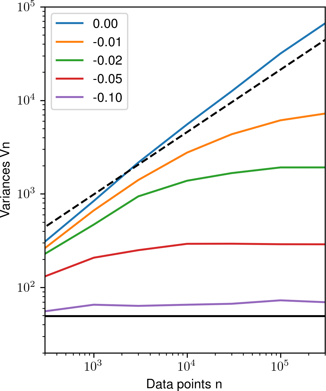
(a) $m=2$

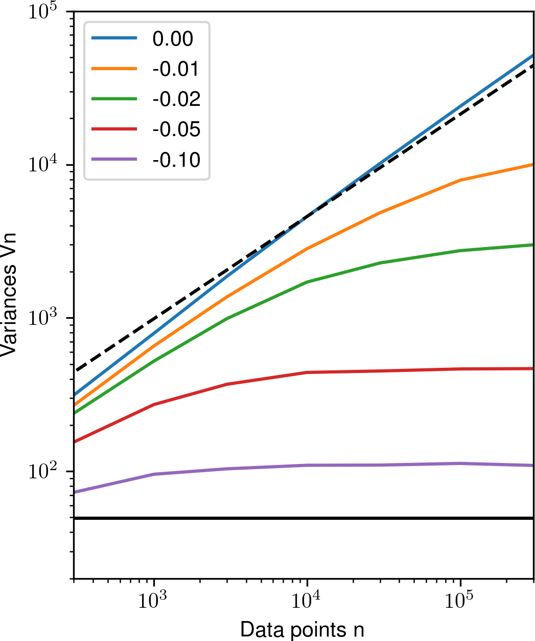
(b) $m=10$

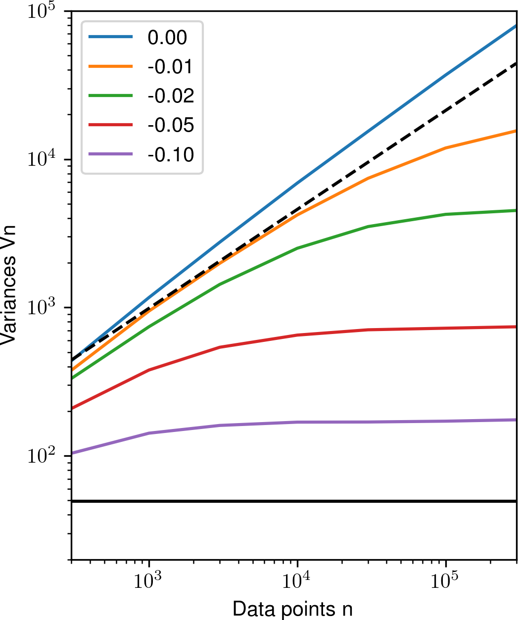
(c) $m=100$

Figure 2: Simulated variances $V$ times $n$ for different values of $\beta$ for dimensions $m=2$, $10$ and $100$. Black lines $V\propto n^{-1}$ (solid) and $V\propto n^{-\frac{1}{3}}$ (dashed) for reference.

The results of our simulation are displayed in Figure 2. The asymptotic rates are clearly in agreement with our considerations based on the asymptotic theory. Strikingly, however, for $\beta<0$ very close to $0$, the decay rate stays close to $n^{-\frac{1}{3}}$ until very large sample sizes and only then settles into the asymptotic rate of $n^{-1}$. This illustrates that the slow convergence to the mean is an issue, which does not only plague the distribution with $\beta=0$ but also sufficiently adjacent distributions for finite sample size.

Even more strikingly, Figure 2 shows that this phenomenon increases with dimension $m$. Indeed, due to Remark 18 (ii), in the limit $m\to\infty$, all derivatives of $G$ vanish with a uniform rate, so that we approach a situation of infinite smeariness.

References

- Afsari (2011) Afsari, B. (2011). Riemannian center of mass: existence, uniqueness, and convexity. Proceedings of the American Mathematical Society 139, 655–773.
- Arnaudon and Miclo (2014) Arnaudon, M. and L. Miclo (2014). Means in complete manifolds: uniqueness and approximation. ESAIM: Probability and Statistics 18, 185–206.
- Bhattacharya and Bhattacharya (2008) Bhattacharya, A. and R. Bhattacharya (2008). Statistics on riemannian manifolds: asymptotic distribution and curvature. Proc. Amer. Math. Soc., 2959–2967.
- Bhattacharya and Lin (2017) Bhattacharya, R. and L. Lin (2017). Omnibus CLT for Fréchet means and nonparametric inference on non-euclidean spaces. to appear.
- Bhattacharya and Patrangenaru (2003) Bhattacharya, R. N. and V. Patrangenaru (2003). Large sample theory of intrinsic and extrinsic sample means on manifolds I. The Annals of Statistics 31(1), 1–29.
- Bhattacharya and Patrangenaru (2005) Bhattacharya, R. N. and V. Patrangenaru (2005). Large sample theory of intrinsic and extrinsic sample means on manifolds II. The Annals of Statistics 33(3), 1225–1259.
- Bhattacharya and Patrangenaru (2013) Bhattacharya, R. N. and V. Patrangenaru (2013). Statistics on manifolds and landmark based image analysis: A nonparametric theory with applications.
- Billera et al. (2001) Billera, L., S. Holmes, and K. Vogtmann (2001). Geometry of the space of phylogenetic trees. Advances in Applied Mathematics 27(4), 733–767.
- Dryden et al. (2009) Dryden, I., A. Koloydenko, and D. Zhou (2009). Non-euclidean statistics for covariance matrices, with applications to diffusion tensor imaging. Annals of Applied Statistics 3(3), 1102–1123.
- Dryden and Mardia (1998) Dryden, I. L. and K. V. Mardia (1998). Statistical Shape Analysis. Chichester: Wiley.
- Ellingson et al. (2013) Ellingson, L., V. Patrangenaru, and F. Ruymgaart (2013). Nonparametric estimation of means on Hilbert manifolds and extrinsic analysis of mean shapes of contours. Journal of Multivariate Analysis 122, 317–333.
- Fletcher and Joshi (2004) Fletcher, P. T. and S. C. Joshi (2004). Principal geodesic analysis on symmetric spaces: Statistics of diffusion tensors. ECCV Workshops CVAMIA and MMBIA, 87–98.
- Fréchet (1948) Fréchet, M. (1948). Les éléments aléatoires de nature quelconque dans un espace distancié. Annales de l’Institut de Henri Poincaré 10(4), 215–310.
- Groisser (2005) Groisser, D. (2005). On the convergence of some Procrustean averaging algorithms. Stochastics: Internatl. J. Probab. Stochstic. Processes 77(1), 51–60.
- Hotz and Huckemann (2015) Hotz, T. and S. Huckemann (2015). Intrinsic means on the circle: Uniqueness, locus and asymptotics. Annals of the Institute of Statistical Mathematics 67(1), 177–193.
- Hotz et al. (2013) Hotz, T., S. Huckemann, H. Le, J. S. Marron, J. Mattingly, E. Miller, J. Nolen, M. Owen, V. Patrangenaru, and S. Skwerer (2013). Sticky central limit theorems on open books. Annals of Applied Probability 23(6), 2238–2258.
- Huckemann (2011a) Huckemann, S. (2011a). Inference on 3D Procrustes means: Tree boles growth, rank-deficient diffusion tensors and perturbation models. Scandinavian Journal of Statistics 38(3), 424–446.
- Huckemann (2011b) Huckemann, S. (2011b). Intrinsic inference on the mean geodesic of planar shapes and tree discrimination by leaf growth. The Annals of Statistics 39(2), 1098–1124.
- Huckemann (2012) Huckemann, S. (2012). On the meaning of mean shape: Manifold stability, locus and the two sample test. Annals of the Institute of Statistical Mathematics 64(6), 1227–1259.
- Huckemann (2015) Huckemann, S. (2015). (Semi-)intrinsic statistical analysis on non-Euclidean spaces. In Advances in Complex Data Modeling and Computational Methods in Statistics. Springer.
- Huckemann et al. (2010) Huckemann, S., T. Hotz, and A. Munk (2010). Intrinsic shape analysis: Geodesic principal component analysis for Riemannian manifolds modulo Lie group actions (with discussion). Statistica Sinica 20(1), 1–100.
- Huckemann et al. (2015) Huckemann, S., J. C. Mattingly, E. Miller, and J. Nolen (2015). Sticky central limit theorems at isolated hyperbolic planar singularities. Electronic Journal of Probability.
- Huckemann and Ziezold (2006) Huckemann, S. and H. Ziezold (2006). Principal component analysis for Riemannian manifolds with an application to triangular shape spaces. Advances of Applied Probability (SGSA) 38(2), 299–319.
- Huckemann and Eltzner (2017) Huckemann, S. F. and B. Eltzner (2017). Backward nested descriptors asymptotics with inference on stem cell differentiation. Annals of Statistics. accepted, arXiv preprint arXiv:1609.00814.
- Jung et al. (2012) Jung, S., I. L. Dryden, and J. S. Marron (2012). Analysis of principal nested spheres. Biometrika 99(3), 551–568.
- Jung et al. (2011) Jung, S., M. Foskey, and J. S. Marron (2011). Principal arc analysis on direct product manifolds. The Annals of Applied Statistics 5, 578–603.
- Karcher (1977) Karcher, H. (1977). Riemannian center of mass and mollifier smoothing. Communications on Pure and Applied Mathematics XXX, 509–541.
- Kendall (1984) Kendall, D. G. (1984). Shape manifolds, Procrustean metrics and complex projective spaces. Bull. Lond. Math. Soc. 16(2), 81–121.
- Kendall et al. (1999) Kendall, D. G., D. Barden, T. K. Carne, and H. Le (1999). Shape and Shape Theory. Chichester: Wiley.
- Kendall (1990) Kendall, W. S. (1990). Probability, convexity, and harmonic maps with small image I: Uniqueness and fine existence. Proceedings of the London Mathematical Society 61, 371–406.
- Le (2001) Le, H. (2001). Locating Fréchet means with an application to shape spaces. Advances of Applied Probability (SGSA) 33(2), 324–338.
- Mardia and Patrangenaru (2005) Mardia, K. and V. Patrangenaru (2005). Directions and projective shapes. The Annals of Statistics 33, 1666–1699.
- Mardia and Jupp (2000) Mardia, K. V. and P. E. Jupp (2000). Directional Statistics. New York: Wiley.
- Marron and Alonso (2014) Marron, J. S. and A. M. Alonso (2014). An overview of object oriented data analysis. Biometrical Journal. to appear.
- McKilliam et al. (2012) McKilliam, R. G., B. G. Quinn, and I. V. L. Clarkson (2012). Direction estimation by minimum squared arc length. IEEE Transactions on Signal Processing 60(5), 2115–2124.
- Moulton and Steel (2004) Moulton, V. and M. Steel (2004). Peeling phylogenetic ’oranges’. Advances in Applied Mathematics 33(4), 710–727.
- Munk et al. (2008) Munk, A., R. Paige, J. Pang, V. Patrangenaru, and F. Ruymgaart (2008). The one- and multi-sample problem for functional data with application to projective shape analysis. Journal of Multivariate Analysis (99), 815–833.
- Patrangenaru and Ellingson (2015) Patrangenaru, V. and L. Ellingson (2015). Nonparametric statistics on manifolds and their applications to object data analysis. CRC Press.
- Pennec (2017) Pennec, X. (2017). Barycentric subspace analysis on manifolds. The Annals of Statistics. accepted, arXiv:1607.02833.
- Sommer (2016) Sommer, S. (2016). Anisotropically weighted and nonholonomically constrained evolutions on manifolds. Entropy 18(12), 425.
- van der Vaart (2000) van der Vaart, A. (2000). Asymptotic statistics. Cambridge Univ. Press.
- Ziezold (1977) Ziezold, H. (1977). Expected figures and a strong law of large numbers for random elements in quasi-metric spaces. Transaction of the 7th Prague Conference on Information Theory, Statistical Decision Function and Random Processes A, 591–602.