Observer-based boundary control of the sine-Gordon model energy

Abstract

In this paper the output feedback energy control problem for the sine-Gordon model is studied. An observer for the sine-Gordon equation and a speed-gradient boundary control law for solving this problem are analysed. Explicit inequalities on system’s parameters ensuring the exponential decay of the estimation error are obtained. Under an additional assumption the achievement of the control goal is proved. The results of numerical experiments demonstrate that the transient time in energy is close to the transient time in observation error.

1 Introduction

This paper is devoted to control of oscillations in nonlinear distributed systems. As the example the celebrated sine-Gordon model was chosen. The sine-Gordon equation is a semilinear wave equation used to model many physical phenomena like Josephson junctions, seismic events including earthquakes, slow slip and after-slip processes, dislocation in solids, etc.[1]. Though control of oscillatory modes is one of conventional areas of control theory, most works in the past were dealing with linear models and regulation or tracking as control objectives. It was motivated by practical problems such as vibration suppression, vibration isolation, etc. [2]. Some of the methods were extended to distributed systems and allowed one to stabilize wave motion [3, 4, 5]. By the beginning of the new century quite a number of control methods for distributed (PDE) systems were proposed for the regulation and tracking problems including optimal control, robust control, adaptive control, etc. [6, 7, 8]. In a number of publications a powerful backstepping method was developed (see [9] and the references therein).

In the 1990s an interest in new problems, related to oscillations shaping and synchronization rather than their suppression was growing [10, 11, 12]. An efficient approach to such problems based on the system speed-gradient and energy control was developed in [13, 14]. Energy is a fundamental characteristics of a physical system which is conserved if the losses can be neglected. Changing the desired level of energy allows one to specify various desired properties of oscillations and describe various system modes. However an approach to energy control proposed in [13, 14] based on the speed-gradient method was not extended to distributed systems and to control of waves until recent. The reason is in that the desired energy level set may be a complex unbounded set with complex geometry.

Perhaps the first attempt to study energy control approach for distributed systems was made in [15] where a possibility of controlling travelling waves in the sine-Gordon model was demonstrated by simulation. In [16] two energy control algorithms were studied rigorously: one provides spatially distributed control action while another one provides a uniform over the space one. Both algorithms, however have some drawbacks. To improve the proposed approach it would be desirable to study the boundary control problem.

The first boundary control algorithms for the sine-Gordon equation were proposed in [17, 18, 19]. In these papers, however, only the stabilization problem was considered. In [20] the boundary control of the sine-Gordon system energy was studied. However the solution proposed in [20] requires measurements of the system velocity which may be not available apart from the boundary of the domain.

In this paper the observer-based solution to the problem of the sine-Gordon model energy boundary control is proposed. The Luenberger-type observer to evaluate velocities required for evaluation of the system energy is proposed. To design the energy control algorithm the speed-gradient method [11] is employed. To analyze the system well-posedness and partial stability an energy-based Lyapunov functional is used. The closed loop dynamics are illustrated by simulation.

The paper is structured as follows. In Section 2 the problem is formulated and necessary notations and definitions are introduced. Control algorithm is designed in Section 3. Section 4 is devoted to studying the properties of the designed control system. Numerical evaluation results are presented in Section 5.

2 Problem Formulation

Consider the one-dimensional sine-Gordon equation with the following initial and boundary conditions

$$z_{tt}(t,x)-kz_{xx}(t,x)+\beta\sin z(t,x)=0,\quad t\geq 0,\quad x\in(0,1)$$ (1)

$$z(0,x)=z^{0}(x),\quad z_{t}(0,x)=z^{1}(x),\quad x\in(0,1),$$ (2)

$$z(t,0)=0,\quad z_{x}(t,1)=u(t),\quad t\geq 0,$$ (3)

$$y(t)=z_{t}(t,1)\quad t\geq 0,$$ (4)

where $\beta>0$ and $k>0$ are given parameters, $u(t)$ is a control input, $y(t)$ is the output, and $z^{0},z^{1}\colon[0,1]\to\mathbb{R}$ are given functions. Denote by

$$H(z)=\int_{0}^{1}\left(\frac{z_{t}^{2}}{2}+k\frac{z_{x}^{2}}{2}+\beta(1-\cos z)\right)\,dx$$

the Hamiltonian for the sine-Gordon equation. One can easily verify that the Hamiltonian $H(z)$ is preserved along solutions of the unforced system. Furthermore, $H(z)$ is a non-negative function, and $H(z)=0$ if and only if $z=0$. Therefore $H(z(t))$ can be viewed as the energy of a solution $z(t,x)$ of equation (1) (or system’s energy) at time $t$.

We pose the following control problem: find a control law $u(t)$, which ensures the control objective

$$H(z(t))\to H^{*}\text{~{}as~{}}t\to+\infty,$$ (5)

where, $z(t)$ is a solution of (1)–(4), and $H^{*}\geq 0$ is prespecified. Thus, the control objective is to reach the desired energy level $H^{*}$ in the system (1)–(4).

Remark 1.

It should be noted that all results below can be easily extended to the case

$$z_{t}(t,1)=u(t),\quad y(t)=z_{x}(t,1)\quad t\geq 0,$$

(i.e. one can swap the input and the output), since the derivatives $z_{t}(t,1)$ and $z_{x}(t,1)$ enter all expressions below almost identically with the only difference being the coefficient $k>0$ before $z_{x}(t,1)$.

3 Speed-Gradient Control Law and Luenberger Type Observer

Let us utilize the Speed-Gradient algorithm in order to design a control law solving the boundary energy control problem posed above. Introduce the goal function

$$Q(z)=\frac{1}{2}\big{(}H(z)-H^{*}\big{)}$$

that measures the difference between the current and the desired energies. The derivative of this function along solutions of the system (1)–(4) has the form

$$\frac{d}{dt}Q(z(t))=(H(z(t))-H^{*})\int_{0}^{1}\Big{(}z_{t}z_{tt}+kz_{x}z_{xt}+\beta\sin zz_{t}\Big{)}\,dx.$$

Substituting $z_{tt}$ for $kz_{xx}-\beta\sin z$ (recall that $z(t)$ is a solution of (1)), and integrating the term $z_{x}z_{xt}$ by parts one obtains

$$\frac{d}{dt}Q(z(t))=(H(z(t))-H^{*})\Bigg{[}\int_{0}^{1}\big{(}z_{t}(kz_{xx}-\beta\sin z)-kz_{xx}z_{t}+\beta\sin zz_{t}\big{)}\,dx\\ +kz_{x}(t,1)z_{t}(t,1)-kz_{x}(t,0)z_{t}(t,0)\Bigg{]}.$$

Hence with the use of the boundary condition $z(t,0)=0$ one finally gets that

$$\frac{d}{dt}Q(z(t))=k(H(z(t))-H^{*})u(t)y(t)$$

Then according to the Speed-Gradient algorithm one defines the control law as follows:

$$u_{0}(t)=-\gamma\frac{\partial}{\partial u}\frac{dQ(z)}{dt}=-\gamma(H(z(t))-H^{*})ky(t),$$

where $\gamma>0$ is a scalar gain. Below, we consider the more general control algorithm of the form

$$u_{0}(t)=-\gamma\psi(H(z(t))-H^{*})y(t),$$ (6)

where $\psi\colon\mathbb{R}\to\mathbb{R}$ is a continuous function such that $\psi(0)=0$ and $\psi(s)s>0$ for any $s\neq 0$.

Note that control law (6) defined with the use of the Speed-Gradient algorithm depends on the current energy of the system $H(z(t))$ that is not available from the measurements. Therefore we need to design an observer. Being inspired by the ideas of [21], we propose a Luenberger-type observer of the form:

$$\widehat{z}_{tt}(t,x)-k\widehat{z}_{xx}(t,x)+\beta\sin\widehat{z}(t,x)=0,\quad t\geq 0,\quad x\in(0,1)$$ (7)

$$\widehat{z}(0,x)=\widehat{z}^{0}(x),\quad\widehat{z}_{t}(0,x)=\widehat{z}^{1}(x),\quad x\in(0,1),$$ (8)

$$\widehat{z}(t,0)=0,\quad\widehat{z}_{x}(t,1)=u(t)+\alpha\big{(}y(t)-\widehat{z}_{t}(t,1)\big{)},\quad t\geq 0,$$ (9)

where $\widehat{z}^{0},\widehat{z}^{1}\colon[0,1]\to\mathbb{R}$ are given functions, and $\alpha>0$ is an observer gain. Now, with the use of the above observer we define the control law as follows:

$$u(t)=-\gamma\psi\Big{(}H(\widehat{z}(t))-H^{*}\Big{)}y(t).$$ (10)

In the following section, we demonstrate that under some additional assumptions control law (10) solves the energy control problem (5).

Remark 2.

Let us note that the observer (7)–(9) can be designed with the use of the Speed-Gradient algorithm as well. Namely, consider the model of the system (1)–(4) of the form

$$\widehat{z}_{tt}(t,x)-k\widehat{z}_{xx}(t,x)+\beta\sin\widehat{z}(t,x)=0,\quad t\geq 0,\quad x\in(0,1)$$

$$\widehat{z}(0,x)=\widehat{z}^{0}(x),\quad\widehat{z}_{t}(0,x)=\widehat{z}^{1}(x),\quad x\in(0,1),$$

$$\widehat{z}(t,0)=0,\quad\widehat{z}_{x}(t,1)=u(t)+\widehat{u}(t),\quad t\geq 0,$$

$$\widehat{y}(t)=\widehat{z}_{t}(t,1).\quad t\geq 0,$$

where $\widehat{u}(t)$ is a control input, and $\widehat{y}(t)$ is the output of the model. Define the goal function

$$\widehat{Q}(\widehat{z})=\int_{0}^{1}\left(\frac{(z_{t}-\widehat{z}_{t})^{2}}{2}+k\frac{(z_{x}-\widehat{z}_{x})^{2}}{2}\right)\,dx,$$

i.e. the goal function is a weighted estimation error. Then one can easily check that applying the Speed-Gradient algorithm in this case we arrive at the control law $\widehat{u}(t)=\alpha(y(t)-\widehat{y}(t))$, which coincides with the one used in (9).

4 Properties of the Designed Control System

Let us study the performance of the system (1)–(4) with control law (10) and observer (7)–(9). The closed-loop system has the from

$$z_{tt}(t,x)-kz_{xx}(t,x)+\beta\sin z(t,x)=0,\quad t\geq 0,\quad x\in(0,1)$$ (11)

$$\widehat{z}_{tt}(t,x)-k\widehat{z}_{xx}(t,x)+\beta\sin\widehat{z}(t,x)=0,\quad t\geq 0,\quad x\in(0,1)$$ (12)

$$z(0,x)=z^{0}(x),\quad z_{t}(0,x)=z^{1}(x),\quad x\in(0,1),$$ (13)

$$\widehat{z}(0,x)=\widehat{z}^{0}(x),\quad\widehat{z}_{t}(0,x)=\widehat{z}^{1}(x),\quad x\in(0,1),$$ (14)

$$z(t,0)=0,\quad z_{x}(t,1)=u(t),\quad t\geq 0,$$ (15)

$$\widehat{z}(t,0)=0,\quad\widehat{z}_{x}(t,1)=u(t)+\alpha\big{(}z_{t}(t,1)-\widehat{z}_{t}(t,1)\big{)},\quad t\geq 0,$$ (16)

$$u(t)=-\gamma\psi\Big{(}H(\widehat{z}(t))-H^{*}\Big{)}z_{t}(t,1)\quad t\geq 0.$$ (17)

Let us introduce an assumption on the well-posedness of this system.

Assumption 1.

There exists a nonempty set $\mathcal{W}_{0}\subseteq W^{2}_{2}(0,1)\times W^{1}_{2}(0,1)$ of “sufficiently smooth” initial data such that for any $(z^{0},z^{1})\in\mathcal{W}_{0}$ and $(\widehat{z}^{0},\widehat{z}^{1})\in\mathcal{W}_{0}$ there exists a unique “sufficiently regular” solution $(z(t,x),\widehat{z}(t,x))$ of the system (11)–(17) such that

1. $(z(t),\widehat{z}(t))$ is defined on a maximal interval of existence $[0,T_{\max})$, and if $T_{\max}<+\infty$, then $H(z(t))+H(\widehat{z}(t))\to+\infty$ as $t\to T_{\max}$,

2. the functions $H(z(\cdot))$ and $H(\widehat{z}(\cdot))$ are locally absolutely continuous.

Remark 3.

Note that for the main results of this paper to hold true it is sufficient (but not necessary) to suppose that

$$z,\widehat{z}\in C\Big{(}[0,T_{\max});W^{2}_{2}(0,1)\Big{)}\cap C^{1}\Big{(}[0,T_{\max});W^{1}_{2}(0,1)\Big{)}\cap C^{2}\Big{(}[0,T_{\max});L_{2}(0,1)\Big{)},$$

where, as in the assumption above, $W^{m}_{p}(0,1)$ is the Sobolev space.

Remark 4.

Let us point out the difficulties in the proof of existence and uniqueness theorem for the initial-boundary value problem (11)–(17). At first, note that this problem cannot be rewritten (without some nontrivial trasformations) as a Lipschitz perturbation of a linear evolution equation of the form

$$\frac{dw}{dt}=\mathcal{A}w+f(w),$$

where $\mathcal{A}$ is an unbounded linear operator in a Banach space $X$. The interested reader can check that regardless of the choice of the space $X$ either the operator $\mathcal{A}$ is not an infinitesimal generator of a $C_{0}$-semigroup or the nonlinear operator $f$ is not locally Lipschitz continuous or $f$ is not defined on the entire space $X$ (or not in the domain of $\mathcal{A}$, so that such results as [22], Theorem 6.1.7 are not applicable). One can consider the problem (11)–(17) as a nonlinear evolution equation, but the corresponding nonlinear operator does not possess any standard properties. It is neither accretive (dissipative) nor compact. Similarly, all other general methods for proving the existence of solutions of nonlinear hyperbolic partial differential equations known to the authors cannot be directly applied to the problem under consideration. Therefore we pose the above assumption on the well-posedness of the system (11)–(17) as a challenging problem for future research. It should be noted that the main difficulty in a proof of this assumption consists in the fact that dynamic boundary conditions (15)–(17) are nondissipative and nonlinearly depend on the derivative $z_{t}(t,1)$.

4.1 Exponential Decay of the Estimation Error

We start our analysis of the control law (10) by showing that under some additional assumptions the equation for the estimation error $e=z-\widehat{z}$ is globally exponentially stable.

Observe that the function $e(t,x)$ is a solution of the following boundary value problem:

$$e_{tt}(t,x)-ke_{xx}(t,x)+\beta\Big{(}\sin z(t,x)-\sin\widehat{z}(t,x)\Big{)}=0,$$ (18)

$$e(0,x)=z^{0}(x)-\widehat{z}^{0}(x),\quad e_{t}(0,x)=z^{1}(x)-\widehat{z}^{1}(x),$$ (19)

$$e(t,0)=0,\quad e_{x}(t,1)=-\alpha e_{t}(t,1),$$ (20)

where $t\geq 0$ and $x\in[0,1]$. Denote by

$$E(t)=\frac{1}{2}\int_{0}^{1}\Big{(}e_{t}^{2}+ke_{x}^{2}\Big{)}\,dx$$

the weighted quadratic error. Our aim is to show that $E(t)$ decays exponentially, provided the parameters $k$ and $\beta$ satisfy certain conditions. In order to conveniently express these conditions, denote

$$\eta(\beta,k)=\max\left\{\beta,\frac{4\beta}{\pi^{2}k-(\pi^{2}+4)\beta}\right\},$$ (21)

and introduce the following assumption.

Assumption 2.

The parameters $k>0$ and $\beta>0$ of the system (1)–(3) satisfy the following inequalities:

$$\left(1+\frac{4}{\pi^{2}}\right)\beta<k,\quad\eta(\beta,k)<\min\big{\{}1,k\big{\}}.$$

One can easily verify that assumption 2 is valid iff

$$\begin{cases}\beta<1,&\text{in the case }k>\dfrac{\pi^{2}+8}{\pi^{2}}\approx 1.81,\\ \beta<\dfrac{\pi^{2}k}{\pi^{2}+8},&\text{in the case }1\leq k\leq\dfrac{\pi^{2}+8}{\pi^{2}},\\ \beta<\dfrac{\pi^{2}k^{2}}{(\pi^{2}+4)k+4},&\text{in the case }0<k<1.\end{cases}$$

Note that for assumption 2 to hold true it is necessary that $\beta<1$.

Theorem 1.

Let Assumptions 1 and 2 be valid. Then for any $\varepsilon>0$ such that $\eta(\beta,k)<\varepsilon<\min\{1,k\}$, and for all $\alpha>0$ satisfying the inequality

$$\frac{\varepsilon k}{2}\alpha^{2}-k\alpha+\frac{\varepsilon}{2}\leq 0$$ (22)

there exist $\delta>0$ and $M>0$ such that for any initial conditions $(z^{0},z^{1})\in\mathcal{W}_{0}$ and $(\widehat{z}^{0},\widehat{z}^{1})\in\mathcal{W}_{0}$, and for all $\gamma>0$ one has

$$E(t)\leq ME(0)e^{-\delta t}\quad\forall t\in[0,T_{\max}).$$

Proof.

For any $\varepsilon>0$ introduce the Lyapunov function

$$V(t)=E(t)+\varepsilon\int_{0}^{1}xe_{t}e_{x}\,dx.$$

(cf. [19], Section 4; [21], Section 2.2). From the inequalities

$$\Big{|}\int_{0}^{1}xe_{t}e_{x}\,dx\Big{|}\leq\int_{0}^{1}|e_{t}||e_{x}|\,dx\leq\frac{1}{2}\int_{0}^{1}e_{t}^{2}\,dx+\frac{1}{2}\int_{0}^{1}e_{x}^{2}\,dx\leq\max\left\{1,\frac{1}{k}\right\}E(t),$$

it follows that for any $\varepsilon<\min\{1,k\}$ one has

$$0\leq(1-k_{0}\varepsilon)E(t)\leq V(t)\leq(1+k_{0}\varepsilon)E(t),\quad(1-k_{0}\varepsilon)>0,$$ (23)

where $k_{0}=\max\{1,1/k\}$. Thus, in particular, for any $0<\varepsilon<\min\{1,k\}$ one has $V(t)\geq 0$.

For any $t\in[0,T_{\max})$ one has

$$\frac{d}{dt}V(t)=\frac{d}{dt}E(t)+\varepsilon\frac{d}{dt}\int_{0}^{1}xe_{t}e_{x}\,dx\\ =\int_{0}^{1}\Big{(}e_{t}e_{tt}+ke_{x}e_{tx}\Big{)}\,dx+\varepsilon\int_{0}^{1}\Big{(}x(e_{tt}e_{x}+e_{t}e_{tx})\Big{)}\,dx.$$ (24)

Taking into account (18) and (20), and integrating by parts one obtains that

$$\frac{d}{dt}E(t)=\int_{0}^{1}\Big{(}e_{t}e_{tt}+ke_{x}e_{tx}\Big{)}\,dx=\int_{0}^{1}\Big{(}e_{t}\big{(}ke_{xx}-\beta\sin z+\beta\sin\widehat{z}\big{)}-ke_{t}e_{xx}\Big{)}\,dx\\ +ke_{x}(t,1)e_{t}(t,1)-ke_{x}(t,0)e_{t}(t,0)=-\alpha ke_{t}(t,1)^{2}+\beta\int_{0}^{1}e_{t}\big{(}\sin\widehat{z}-\sin z\big{)}\,dx.$$

Applying the fact that the function $y\to\sin y$ is globally Lipschitz continuous with the Lipschitz constant $L=1$ one gets that

$$\Big{|}\int_{0}^{1}e_{t}\big{(}\sin\widehat{z}-\sin z\big{)}\,dx\Big{|}\leq\int_{0}^{1}|e_{t}||e|\,dx\leq\frac{1}{2}\int_{0}^{1}e_{t}^{2}\,dx+\frac{1}{2}\int_{0}^{1}e^{2}\,dx.$$

Hence with the use of Wirtinger’s inequality (see, e.g., [23]) one obtains that

$$\frac{d}{dt}E(t)\leq-\alpha ke_{t}(t,1)^{2}+\frac{\beta}{2}\int_{0}^{1}e_{t}^{2}\,dx+\frac{2\beta}{\pi^{2}}\int_{0}^{1}e_{x}^{2}\,dx.$$ (25)

Now, let us consider the second term in (24). At first, note that

$$\int_{0}^{1}xe_{t}e_{tx}\,dx=\frac{1}{2}\int_{0}^{1}\Big{(}\frac{d}{dx}\big{(}xe_{t}^{2}\big{)}-e_{t}^{2}\Big{)}\,dx=\frac{1}{2}e_{t}(t,1)^{2}-\frac{1}{2}\int_{0}^{1}e_{t}^{2}\,dx$$ (26)

At second, applying (18) and (20) one finds that

$$\int_{0}^{1}xe_{x}e_{tt}\,dx=\int_{0}^{1}xe_{x}\Big{(}ke_{xx}-\beta\sin z+\beta\sin\widehat{z}\Big{)}\,dx\\ \leq\frac{k}{2}\int_{0}^{1}\Big{(}\frac{d}{dx}\big{(}xe_{x}^{2}\big{)}-e_{x}^{2}\Big{)}\,dx+\beta\int_{0}^{1}x|e_{x}||e|\,dx\\ \leq-\frac{k}{2}\int_{0}^{1}e_{x}^{2}\,dx+\frac{k}{2}e_{x}^{2}(t,1)+\frac{\beta}{2}\int_{0}^{1}e_{x}^{2}\,dx+\frac{\beta}{2}\int_{0}^{1}e^{2}\,dx\\ \leq\left(-\frac{k}{2}+\frac{\beta}{2}+\frac{2\beta}{\pi^{2}}\right)\int_{0}^{1}e_{x}^{2}\,dx+\frac{k}{2}\alpha^{2}e_{t}^{2}(t,1).$$ (27)

Combining (24)–(27) one gets that for any $t\in[0,T_{\max})$ the following inequality holds true

$$\frac{d}{dt}V(t)\leq\left(-\frac{\varepsilon}{2}+\frac{\beta}{2}\right)\int_{0}^{1}e_{t}^{2}\,dx+\left(-\frac{\varepsilon k}{2}+\frac{2\beta}{\pi^{2}}+\frac{\varepsilon\beta}{2}+\frac{2\varepsilon\beta}{\pi^{2}}\right)\int_{0}^{1}e_{x}^{2}\,dx\\ +\Big{(}-\alpha k+\frac{\varepsilon}{2}+\frac{\varepsilon k}{2}\alpha^{2}\Big{)}e_{t}^{2}(t,1).$$

Denote

$$\delta_{1}(\varepsilon)=-\frac{\varepsilon}{2}+\frac{\beta}{2},\quad\delta_{2}(\varepsilon)=-\frac{\varepsilon k}{2}+\frac{2\beta}{\pi^{2}}+\frac{\varepsilon\beta}{2}+\frac{2\varepsilon\beta}{\pi^{2}},$$ (28)

$$\delta_{3}(\varepsilon,\alpha)=-\alpha k+\frac{\varepsilon}{2}+\frac{\varepsilon k}{2}\alpha^{2}.$$ (29)

Then the above inequality can be rewritten as follows

$$\frac{d}{dt}V(t)\leq\delta_{1}(\varepsilon)\int_{0}^{1}e_{t}^{2}\,dx+\delta_{2}(\varepsilon)\int_{0}^{1}e_{x}^{2}\,dx+\delta_{3}(\varepsilon,\alpha)e_{t}^{2}(t,1).$$

Our aim is to show that under the assumptions of the theorem for any $\varepsilon>0$ and $\alpha>0$ satisfying the inequalities

$$\eta(\beta,k)<\varepsilon<\min\{1,k\},\quad\delta_{3}(\varepsilon,\alpha):=\frac{\varepsilon k}{2}\alpha^{2}-k\alpha+\frac{\varepsilon}{2}\leq 0$$

one has $\delta_{1}(\varepsilon)<0$ and $\delta_{2}(\varepsilon)<0$. Then for any such $\varepsilon$ and $\alpha$ one has

$$\frac{d}{dt}V(t)\leq-\min\left\{2|\delta_{1}(\varepsilon)|,\frac{2|\delta_{2}(\varepsilon)|}{k}\right\}E(t).$$

Consequently, applying (23) one gets that

$$\frac{d}{dt}V(t)\leq-\delta(\varepsilon)V(t),\quad\delta(\varepsilon)=\min\left\{\frac{2|\delta_{1}(\varepsilon)|}{1+k_{0}\varepsilon},\frac{2|\delta_{2}(\varepsilon)|}{k(1+k_{0}\varepsilon)}\right\}>0,$$

which yeilds $V(t)\leq V(0)e^{-\delta(\varepsilon)t}$ for all $t\in[0,T_{\max})$. Hence and from (23) it follows that

$$E(t)\leq\frac{1+k_{0}\varepsilon}{1-k_{0}\varepsilon}E(0)e^{-\delta(\varepsilon)t}\quad\forall t\in[0,T_{\max}),$$ (30)

which implies the required result.

Thus, it remains to show that for any $\varepsilon>0$ and $\alpha>0$ such that

$$\eta(\beta,k)<\varepsilon<\min\{1,k\},\quad\delta_{3}(\varepsilon,\alpha)\leq 0$$

one has $\delta_{1}(\varepsilon)<0$ and $\delta_{2}(\varepsilon)<0$. From (28) it follows that $\varepsilon\in(0,\min\{1,k\})$ such that $\delta_{1}(\varepsilon)<0$ and $\delta_{2}(\varepsilon)<0$ exists if and only if

$$\min\{1,k\}>\beta,\quad-k+\left(1+\frac{4}{\pi^{2}}\right)\beta<0,\quad\min\{1,k\}>\frac{4\beta}{\pi^{2}k-(\pi^{2}+4)\beta}$$

or, equivalently, $(1+4/\pi^{2})\beta<k$ and $\eta(\beta,k)<\min\{1,k\}$ (see (21)). The above inequalities are valid due to assumption 2. Therefore for any $\varepsilon>0$ such that $\eta(\beta,k)<\varepsilon<\min\{1,k\}$ one has $\delta_{1}(\varepsilon)<0$ and $\delta_{2}(\varepsilon)<0$. Choosing $\alpha>0$ such that $\delta_{3}(\varepsilon,\alpha)\leq 0$ (note that such $\alpha$ exists, if $\varepsilon<k$; see (22)) one obtains the required result. ∎

Remark 5.

The same observer as (7)–(9) was studied in [21] for the uncontrolled system of the form (1)–(4). It should be noted that sufficient conditions for the exponential decay of the weighted quadratic error $E(t)$ were formulated in [21] in terms of the feasibility of certain LMIs simultaneously depending on system’s parameters $k$ and $\beta$, and the observer gain $\alpha$. In contrast, in this paper explicit inequalities on system’s parameters $k$ and $\beta$ and the observer gain $\alpha$ ensuring the exponential decay of $E(t)$ are obtained. The region of admissible (i.e. satisfying assumption 2) parameters $k$ and $\beta$ is shown on Fig. 1.

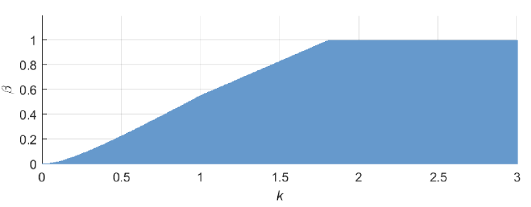
Figure 1: The region of admissible parameters $k$ and $\beta$.

Note that for any $k$ and $\beta$ from this region one can choose the observer gain $\alpha$ for which the weighted quadratic error $E(t)$ decays exponentially.

4.2 Global Well-Posedness of the Closed-Loop System

At the second step, let us show that a solution $(z(t),\widehat{z}(t))$ of the system (11)–(17) is defined on $[0,+\infty)$, i.e. $T_{\max}=+\infty$. With the use of this result we will show that $|H(\widehat{z}(t))-H(z(t))|\to 0$ as $t\to\infty$.

Theorem 2.

Let Assumptions 1 and 2 be valid. Then for any $\varepsilon>0$ such that $\eta(\beta,k)<\varepsilon<\min\{1,k\}$, for all $\alpha>0$ satisfying (22), for all $\gamma>0$, and for any initial conditions $(z^{0},z^{1})\in\mathcal{W}_{0}$ and $(\widehat{z}^{0},\widehat{z}^{1})\in\mathcal{W}_{0}$ there exists $H_{\max}>0$ such that

$$H(z(t))\leq H_{\max},\quad H(\widehat{z}(t))\leq H_{\max}\quad\forall t\in[0,T_{\max}),$$ (31)

which implies that the system is forward complete $(\text{i.e.~{}}T_{\max}=+\infty)$.

Proof.

Denote by $\|\cdot\|$ the standard norm in $L_{2}(0,1)$, and let $(z(t),\widehat{z}(t))$ be a solution of (11)–(17). For any $t\in[0,T_{\max})$ one has

$$\|z_{t}(t)\|\leq\|z_{t}(t)-\widehat{z}_{t}(t)\|+\|\widehat{z}_{t}(t)\|\leq\sqrt{2E(t)}+\sqrt{2H(\widehat{z}(t))}.$$

Hence and from Theorem 1 it follows that there exist $M>0$ and $\delta>0$ such that for any $t\in[0,T_{\max})$ the following inequality holds true:

$$\|z_{t}(t)\|^{2}\leq 4E(t)+4H(\widehat{z}(t))\leq 4ME(0)e^{-\delta t}+4H(\widehat{z}(t)).$$

Similarly, for any $t\in[0,T_{\max})$ one has

$$\|z_{x}(t)\|^{2}\leq\frac{4}{k}ME(0)e^{-\delta t}+\frac{4}{k}H(\widehat{z}(t)).$$

Therefore for all $t\in[0,T_{\max})$ one has

$$H(z(t))\leq\frac{1}{2}\|z_{t}(t)\|^{2}+\frac{k}{2}\|z_{x}(t)\|^{2}+2\beta\leq C_{1}+C_{2}H(\widehat{z}(t)),$$ (32)

where $C_{1}=2\beta+4ME(0)$ and $C_{2}=4$. Arguing in the same way one can easily verify that

$$H(\widehat{z}(t))\leq C_{1}+C_{2}H(z(t))\quad\forall t\in[0,T_{\max}).$$ (33)

Let $t_{0}\in[0,T_{\max})$ be arbitrary. If $H(\widehat{z}(t_{0}))\leq H^{*}$, then $H(z(t_{0}))\leq C_{1}+C_{2}H^{*}$ due to (32). Suppose, now, that $H(\widehat{z}(t_{0}))>H^{*}$. If $H(\widehat{z}(t))>H^{*}$ for all $t\in[0,t_{0}]$, then $H(z(t))\leq H(z(0))$ for any $t\in[0,t_{0}]$ and $H(\widehat{z}(t_{0}))\leq C_{1}+C_{2}H(z(0))$ due to (33) and the fact that

$$\frac{d}{dt}H(z(t))=-\gamma k\psi(H(\widehat{z}(t))-H^{*})z_{t}(t,1)^{2}\leq 0$$ (34)

for all $t\in[0,t_{0})$ (see the definition of $\psi(s)$).

On the other hand, if $H(\widehat{z}(t_{0}))>H^{*}$, but there exists $t\in[0,t_{0}]$ such that $H(\widehat{z}(t_{0}))\leq H^{*}$, then denote $\tau=\sup\{t\in[0,t_{0}]\mid H(\widehat{z}(t))=H^{*}\}$. Observe that $\tau$ is correctly defined and $\tau<t_{0}$ due to the fact that the function $H(\widehat{z}(t))$ is continuous by our assumptions on the well-posedness of the closed-loop system. Furthermore, for any $t\in[\tau,t_{0}]$ one has $H(\widehat{z}(t))>H^{*}$. Taking into account (32), (34) and the definition of $\tau$ one gets that $H(z(t))\leq H(z(\tau))\leq C_{1}+C_{2}H^{*}$ for any $t\in[\tau,t_{0}]$, which with the use of (33) implies that

$$H(\widehat{z}(t_{0}))\leq C_{1}+C_{2}H(z(t_{0}))\leq C_{1}+C_{1}C_{2}+C_{2}^{2}H^{*}.$$

Since $t_{0}\in[0,T_{\max})$ was chosen arbitrarily, one obtains that $H(z(t))\leq H_{\max}$ and $H(\widehat{z}(t))\leq H_{\max}$ for all $t\in[0,T_{\max})$, where

$$H_{\max}=\max\Big{\{}H^{*},H(z(0)),C_{1}+C_{2}H^{*},C_{1}+C_{2}H(z(0)),C_{1}+C_{1}C_{2}+C_{2}^{2}H^{*}\Big{\}}.$$

It remains to note that the boundedness of $H(z(t))$ and $H(\widehat{z}(t))$ implies that $T_{\max}=+\infty$ by virtue of our assumption on the well-posedness of the closed-loop system. ∎

Corollary 1.

Let Assumptions 1 and 2 be valid. Then for any $\varepsilon>0$ such that $\eta(\beta,k)<\varepsilon<\min\{1,k\}$, for all $\alpha>0$ satisfying (22), for all $\gamma>0$, and for any initial conditions $(z^{0},z^{1})\in\mathcal{W}_{0}$ and $(\widehat{z}^{0},\widehat{z}^{1})\in\mathcal{W}_{0}$ there exist $C$ and $\delta>0$ such that

$$\big{|}H(z(t))-H(\widehat{z}(t))\big{|}\leq C\sqrt{E(0)}e^{-\delta t/2}\quad\forall t\geq 0.$$ (35)

Proof.

Let $H_{\max}>0$ be from the theorem above. Then for any $t\geq 0$ one has

$$\max\Big{\{}\|z_{t}(t)\|,\|z_{x}(t)\|,\|\widehat{z}_{t}(t)\|,\|\widehat{z}_{x}(t)\|\Big{\}}\leq C_{1}:=\sqrt{\max\left\{2,\frac{2}{k}\right\}H_{\max}}.$$

Hence applying the fact that the function $f(s)=s^{2}/2$ is Lipschitz continuous on $[-C_{1},C_{1}]$ with the Lipschitz constant $L=C_{1}$ one obtains that

$$\left|\frac{1}{2}\|z_{t}(t)\|^{2}-\frac{1}{2}\|\widehat{z}_{t}(t)\|^{2}\right|\leq C_{1}\|z_{t}(t)-\widehat{z}_{t}(t)\|\leq C_{1}\sqrt{2E(t)}\quad\forall t\geq 0,$$ (36)

and

$$\left|\frac{k}{2}\|z_{x}(t)\|^{2}-\frac{k}{2}\|\widehat{z}_{x}(t)\|^{2}\right|\leq C_{1}k\|z_{x}(t)-\widehat{z}_{x}(t)\|\leq C_{1}\sqrt{\frac{2}{k}E(t)}\quad\forall t\geq 0.$$ (37)

Note that since $z(t,0)=\widehat{z}(t,0)=0$, for any $x\in(0,1)$ one has

$$|z(t,x)-\widehat{z}(t,x)|=\Big{|}\int_{0}^{x}\big{(}z_{x}(t,y)-\widehat{z}_{x}(t,y)\big{)}\,dy\Big{|}\leq\|z_{x}(t)-\widehat{z}_{x}(t)\|.$$

Hence and from the fact that the function $f(s)=1-\cos(s)$ is Lipschitz continuous with the Lipschitz constant $L=1$ it follows that

$$\Big{|}\int_{0}^{1}\big{(}\beta(1-\cos z(t,x))-\beta(1-\cos\widehat{z}(t,x))\big{)}\,dx\Big{|}\\ \leq\beta\int_{0}^{1}|z(t,x)-\widehat{z}(t,x)|\,dx\leq\beta\|z_{x}(t)-\widehat{z}_{x}(t)\|\leq\beta\sqrt{\frac{2}{k}E(t)}.$$

Combining (36), (37) and the inequality above one gets that there exists $C_{2}>0$ such that $|H(z(t))-H(\widehat{z}(t))|\leq C_{2}\sqrt{E(t)}$ for all $t\geq 0$. Now, applying Theorem 1 we arrive at the required result. ∎

4.3 Performance of the Control System

Now, we are ready to prove that control law (10) indeed solves the energy control problem (5).

Theorem 3.

Let Assumptions 1 and 2 be valid. Then for all $H^{*}>0$ and $\gamma>0$, for any $\varepsilon>0$ such that $\eta(\beta,k)<\varepsilon<\min\{1,k\}$, for all $\alpha>0$ satisfying (22), and for any initial conditions $(z^{0},z^{1})\in\mathcal{W}_{0}$ and $(\widehat{z}^{0},\widehat{z}^{1})\in\mathcal{W}_{0}$ such that $H(z(0))\neq 0$ and $H(z(t))\neq 0$ for all $t\geq 0$ one has $H(z(t))\to H^{*}$ as $t\to\infty$.

Proof.

For any $\varepsilon>0$ introduce the Lyapunov-like function

$$V(t)=H(z(t))+\varepsilon\operatorname{sign}(H(z(t))-H^{*})g(t),\quad g(t)=\int_{0}^{1}xz_{t}z_{x}\,dx.$$

With the use of the inequalities

$$\Big{|}\int_{0}^{1}xz_{t}z_{x}\,dx\Big{|}\leq\int_{0}^{1}|z_{t}z_{x}|\,dx\\ \leq\frac{1}{2}\int_{0}^{1}z_{t}^{2}\,dx+\frac{1}{2}\int_{0}^{1}z_{x}^{2}\,dx,$$

one gets that

$$0\leq(1-\varepsilon k_{0})H(z(t))\leq V(t)\leq(1+\varepsilon k_{0})H(z(t))$$ (38)

for all $t\geq 0$ and $\varepsilon<\min\{1,k\}$, where $k_{0}=\max\{1,1/k\}$.

Fix arbitrary $t\geq 0$ such that $H(z(t))\neq H^{*}$. One has

$$\frac{d}{dt}g(t)=\int_{0}^{1}\big{(}xz_{tt}z_{x}+xz_{t}z_{tx}\big{)}\,dx=\int_{0}^{1}\big{(}x(kz_{xx}-\beta\sin z)z_{x}+xz_{t}z_{tx}\big{)}\,dx.$$

Note that

$$\int_{0}^{1}xz_{t}z_{tx}\,dx=\frac{1}{2}\int_{0}^{1}x(z_{t}^{2})_{x}\,dx=\frac{1}{2}z_{t}(t,1)^{2}-\frac{1}{2}\int_{0}^{1}z_{t}^{2}\,dx$$

and

$$\int_{0}^{1}xz_{xx}z_{x}\,dx=\frac{1}{2}\int_{0}^{1}x(z_{x}^{2})_{x}\,dx=\frac{1}{2}z_{x}(t,1)^{2}-\frac{1}{2}\int_{0}^{1}z_{x}^{2}\,dx.$$

Observe also that

$$-\int_{0}^{1}x\sin zz_{x}\,dx=\int_{0}^{1}x(\cos z)_{x}\,dx=\cos z(t,1)-\int_{0}^{1}\cos z\,dx\\ \leq\int_{0}^{1}(1-\cos z)\,dx\leq\frac{1}{2}\int_{0}^{1}z^{2}\,dx\leq\frac{2}{\pi^{2}}\int_{0}^{1}z_{x}^{2}\,dx.$$

Here we used Wirtinger’s inequality (see [23]). Hence for any $\sigma>0$ one has

$$\frac{d}{dt}g(t)\leq-\int_{0}^{1}\left(\frac{z_{t}^{2}}{2}+k\frac{z_{x}^{2}}{2}\right)\,dx+\frac{1}{2}z_{t}^{2}(t,1)+\frac{k}{2}z_{x}^{2}(t,1)\\ +\beta\int_{0}^{1}(1-\cos z)\,dx\leq-\frac{1}{2}\int_{0}^{1}z_{t}^{2}\,dx-\frac{k}{2}\left(1-\frac{4(1+\sigma)\beta}{k\pi^{2}}\right)\int_{0}^{1}z_{x}^{2}\,dx\\ -\sigma\beta\int_{0}^{1}(1-\cos z)\,dx+\frac{1}{2}z_{t}^{2}(t,1)+\frac{k}{2}z_{x}^{2}(t,1).$$

Since $0\leq\beta<k\pi^{2}/4$ by virtue of Assumption 2, there exists $\sigma>0$ such that

$$C_{0}:=\min\left\{\sigma,1-\frac{4(1+\sigma)\beta}{k\pi^{2}}\right\}>0.$$

Thus, one gets

$$\frac{d}{dt}g(t)\leq-C_{0}H(z(t))+\frac{1}{2}z_{t}^{2}(t,1)+\frac{k}{2}z_{x}^{2}(t,1).$$ (39)

Observe also that

$$\frac{d}{dt}V(t)=-\gamma k\psi(H(\widehat{z}(t))-H^{*})z_{t}^{2}(t,1)+\varepsilon\operatorname{sign}(H(z(t))-H^{*})\frac{d}{dt}g(t)$$ (40)

for any $t\geq 0$ such that $H(z(t))\neq H^{*}$.

Fix an arbitrary $\Delta>0$. Let us show that for any $T>0$ there exists $t\geq T$ such that $|H(z(t))-H^{*}|<\Delta$. Indeed, arguing by reductio ad absurdum, suppose that there exists $T>0$ such that for any $t\geq T$ one has $|H(z(t))-H^{*}|\geq\Delta$. Let us first consider the case when $H(z(t))\geq H^{*}+\Delta$ for all $t\geq T$.

From Corollary 1 it follows that there exists $\tau\geq T$ such that

$$\big{|}H(z(t))-H(\widehat{z}(t))\big{|}\leq\frac{\Delta}{2}\quad\forall t\geq\tau,$$

which implies that $H(\widehat{z}(t))\geq H^{*}+\Delta/2$ for all $t\geq\tau$. Define

$$\psi_{\Delta}=\min\left\{\psi(s)\Bigm{|}s\in\left[\frac{\Delta}{2},K\right]\right\}>0,$$

$$\Psi_{\Delta}=\max\left\{\psi(s)\Bigm{|}s\in\left[\frac{\Delta}{2},K\right]\right\}<+\infty,$$

where $K>0$ is a sufficiently large constant such that $H(\widehat{z}(t))\leq H^{*}+K$ for all $t\geq 0$ that exists by virtue of Theorem 2. By the definitions of $\tau$, $\psi_{\Delta}$ and $\Psi_{\Delta}$ one has $0<\psi_{\Delta}\leq\psi(H(\widehat{z}(t))-H^{*})\leq\Psi_{\Delta}<+\infty$ for all $t\geq\tau$. Applying (39), (40) and the above inequality one obtains that for any $t\geq\tau$ the following inequality holds true

$$\frac{d}{dt}V(t)\leq-\varepsilon C_{0}H(z(t))-\gamma k\psi_{\Delta}z_{t}^{2}(t,1)+\frac{\varepsilon}{2}z_{t}^{2}(t,1)+\frac{\varepsilon k}{2}\gamma^{2}\Psi_{\Delta}^{2}z_{t}^{2}(t,1).$$

Choosing $\varepsilon>0$ sufficiently small and taking into account (38) one gets that

$$\frac{d}{dt}V(t)\leq-\varepsilon C_{0}H(z(t))\leq-C_{\varepsilon}V(t)\quad\forall t\geq\tau,$$

where $C_{\varepsilon}=\varepsilon C_{0}/(1+\varepsilon k_{0})$. Therefore $V(t)\leq V(\tau)e^{-C_{\varepsilon}(t-\tau)}$ for any $t\geq\tau$, which, due to (38), implies that

$$H(z(t))\leq\frac{V(\tau)}{1-\varepsilon k_{0}}e^{-C_{\varepsilon}(t-\tau)}\quad\forall t\geq\tau.$$

Thus, $H(z(t))\to 0$ as $t\to\infty$, which contradicts our assumption that $H(z(t))\geq H^{*}+\Delta$ for any $t\geq T$.

Suppose, now, that $H(z(t))<H^{*}-\Delta$ for all $t\geq T$. Arguing in a similar way to the case $H(z(t))>H^{*}+\Delta$, and applying (39) and (40) one can verify that for any sufficiently small $\varepsilon>0$ there exist $\tau\geq T$ and $C_{\varepsilon}>0$ such that $V(t)\geq V(\tau)e^{C_{\varepsilon}(t-\tau)}$ for any $t\geq\tau$. Hence with the use of (38) one gets that

$$H(z(t))\geq\frac{1-\varepsilon k_{0}}{1+\varepsilon k_{0}}H(z(\tau))e^{-C_{\varepsilon}t}\quad\forall t\geq\tau.$$

By our assumption $H(z(\tau))>0$. Consequently, $H(z(t))\to+\infty$ as $t\to\infty$, which contradicts the assumption that $H(z(t))<H^{*}-\Delta$ for all $t\geq T$. Thus, for any $T>0$ there exists $t\geq T$ such that $|H(z(t))-H^{*}|<\Delta$.

Let $\tau>0$ be such that $|H(z(t))-H(\widehat{z}(t))|\leq\Delta/2$ for all $t\geq\tau$ (see Corollary 1). As we have just proved, there exists $t_{0}\geq\tau$ such that $|H(z(t_{0}))-H^{*}|<\Delta$. Let us verify that

$$\big{|}H(z(t))-H^{*}\big{|}\leq\Delta\quad\forall t\geq t_{0}.$$ (41)

Then one can conclude that $H(z(t))\to H^{*}$ as $t\to\infty$. Arguing by reductio ad absurdum, suppose that there exists $T\geq t_{0}$ such that $|H(z(T))-H^{*}|>\Delta$. Let us consider the case $H(z(T))>H^{*}+\Delta$ first. Define

$$\theta=\sup\Big{\{}t\in[t_{0},T]\Bigm{|}H(z(t))=H^{*}+\Delta\Big{\}}.$$

Note that $\theta$ is correctly defined, and $\theta\in(t_{0},T)$, since $H(z(t))$ is continuous by our assumption. From the definition of $\tau$ and $\theta$ it follows that $H(\widehat{z}(t))\geq H^{*}+\Delta/2$ for any $t\in[\theta,T]$. Therefore

$$\frac{d}{dt}H(z(t))=-\gamma k\psi\big{(}H(\widehat{z}(t))-H^{*}\big{)}z_{t}^{2}(t,1)\leq 0\quad\forall t\in[\theta,T].$$

Consequently, $H(z(T))\leq H(z(\theta))=H^{*}+\Delta$, which condtradicts the definition of $T$.

Suppose, now, that $H(z(T))<H^{*}-\Delta$. Define

$$\theta=\sup\Big{\{}t\in[t_{0},T]\Bigm{|}H(z(t))=H^{*}-\Delta\Big{\}}.$$

Taking into account the definition of $\tau$ and the fact that $t_{0}\geq\tau$ one gets that $H(\widehat{z}(t))\leq H^{*}-\Delta/2$ for any $t\in[\theta,T]$, which implies that

$$\frac{d}{dt}H(z(t))=-\gamma k\psi\big{(}H(\widehat{z}(t))-H^{*}\big{)}z_{t}^{2}(t,1)\geq 0\quad\forall t\in[\theta,T].$$

Therefore, $H(z(T))\geq H(z(\theta))=H^{*}-\Delta$, which contradicts the definition of $T$. Thus, (41) holds true, and $H(z(t))\to H^{*}$ as $t\to\infty$ due to the fact that $\Delta>0$ was chosen arbitrarily. ∎

Remark 6.

In the theorem above we utilized the assumption that $H(z(t))\neq 0$ for all $t\geq 0$ (which, in essence, means that $z(0)\neq 0\implies z(t)\neq 0$ for all $t\geq 0$). With the use of Corollary 1 one can verify that this assumption is satisfied, in particular, if the initial conditions of the observer $(\widehat{z}^{0},\widehat{z}^{1})$ are sufficiently close to the initial conditions $(z^{0},z^{1})$. However, both of these assumptions seem artificial. Note that the implication $H(z(0))\neq 0\implies H(z(t))\neq 0$ for all $t\geq 0$ can be easily established if, in particular, solutions of the closed-loop system (11)–(17) are locally unique. Furthermore, even if the local existence and uniqueness theorem is not available (which is the case), it seems unnatural to expect the control law $u(t)=-\gamma\psi(H(\widehat{z}(t))-H^{*})z_{t}(t,1)$, with $H(\widehat{z}(t))$ being bounded, to steer the state of the system (1)–(4) to the origin in finite time. However, the authors were unable to prove this result rigorously.

5 Numerical evaluation results

The closed-loop energy control system with plant model (2)–(4), observer (7)–(9) and controller (10) was numerically studied by the simulation in MATLAB/Simulink software environment. The computation method and simulation results are described below.

5.1 Computation method

The PDE equations of the plant model (1)–(4) and observer (7)–(9) are approximately represented as ODE systems by discretization on a spatial variable $x$ and implemented by two separate Simulink blocks.

Consider the discretization procedure for plant model (2)–(4). The procedure for observer (7)–(9) is a similar one with the exception of the boundary conditions.

In the numerical study, the partial differential equation (2) is discretized in the spatial variable $x\in\mathbb{R}^{1}$ by uniformly splitting the segment $[0,1]$ into $N$ sub-intervals. The resulting system of $N-1$ ordinary differential equations (ODEs) of the second order is solved over a time interval $[0,T]$ by applying the variable step Runge–Kutta Method [24], performed with the standard MATLAB routine ode45.

At the discretization nodes $x_{i}=i\cdot h$, $i=1,\dots,N-1$, the second-order spatial derivatives of $z(t,x)$ are approximately computed as

$$\begin{array}[]{l}z_{xx}(t,x_{i})=\dfrac{z(t,x_{i+1})-2z(t,x_{i})+z(t,x_{i-1})}{h^{2}},\quad\text{for}~{}~{}2\leq i\leq N-2,\\ z_{xx}(t,x_{1})=\dfrac{z(t,x_{2})-2z(t,x_{1})+z(t,x_{0})}{h^{2}},\\ z_{xx}(t,x_{N-1})=\dfrac{z(t,x_{N})-2z(t,x_{N-1})+z(t,x_{N-2})}{h^{2}},\end{array}$$ (45)

where $h=1/N$ is the discretization step; $z(t,x_{0})$ and $z(t,x_{N})$ correspond to the boundary values of the PDEs and are calculated outside the ODE solver procedure. The value of $z(t,x_{0})$ is taken in accordance with (3) as $z(t,x_{0})=z(t,0)=0$. The value of $z(t,x_{N})$ includes the boundary control $u(t)$ and, as follows from (3), is calculated as $z(t,x_{N})=z(t,x_{N-1})+h\,u(t)$. The plant output $y(t)$ is found in accordance with (4) as $y(t)=z_{t}(t,x_{N-1})$. The remaining values $z(t,x_{1})$, …, $z(t,x_{N-1})$ are computed by numerical solving the following $(N-1)$ ODE equations of the second order:

$$z_{tt}(t,x_{i})=kz_{xx}(t,x_{i})-\beta\sin\big{(}z(t,x_{i})\big{)},\quad 1\leq i\leq N-1$$ (46)

with the given initial (2) and boundary (3) conditions.

The similar procedure is used for ODE representation of the observer equation (7) with the exception that boundary value $\widehat{z}(t,x_{N})$ is found as $\widehat{z}(t,x_{N})=\widehat{z}(t,x_{N-1})+h\left(u(t)+\alpha\big{(}y(t)-\widehat{z}_{t}(t,x_{N-1}\big{)}\right)$, see (9), and the initial conditions are defined by (8).

Simulink blocks for plant (2)–(4) and observer (7)–(9) models are connected by the measurement relation $y(t)=z_{t}(t,x_{N-1})$ and controller (10) equation.

5.2 Simulation results

The following parameters were used in the simulation: $k=0.12$, $\beta=0.02$ and $\alpha=20$. Initial conditions (3) were set to: $z^{0}(x)=5(1-\cos(2\pi x))$, $z^{1}(x)=0$. For observer (7)–(9) zero initial conditions were taken. The desirable energy level was chosen as $H^{*}=10$. The simulation time was confined to $50$. For simulations, the system of PDEs was uniformly discretized in the spacial variable $x$ on $N=1000$ intervals.

The simulation results are depicted in Figs. 2–7. The observer behaviour is illustrated by Figs. 2–5. The spatial-temporal plot of the observation error $e(t,x)=z(t,x)-\widehat{z}(t,x)$ is shown in Fig. 2. Fig. 3 demonstrates observer weighted quadratic error $E(t)$ time history. As is seen from the plots, the observation error decays exponentially with the transient time about $30$ time units.

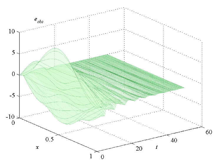
Figure 2: The spatial-temporal plot of the observation error $e(t,x)$.

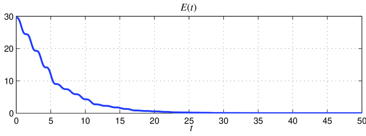
Figure 3: Weighted quadratic error $E(t)$ time history.

Figures 4, 5 demonstrate the estimation of $z(t,x)$, $z_{t}(t,x)$ for the particular point $x=0.5$ (the middle of the spatial interval $x\in[0,1]$). The plots show that the transient response time of the observation error is the same.

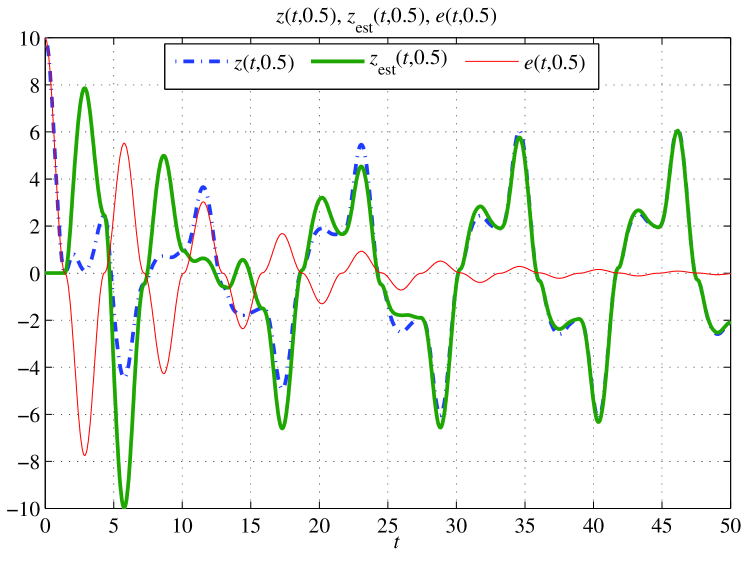
Figure 4: Process of $z(t,x)$ estimation for $x=0.5$. $z(t,0.5)$ and $\hat{z}(t,0.5)$ time histories.

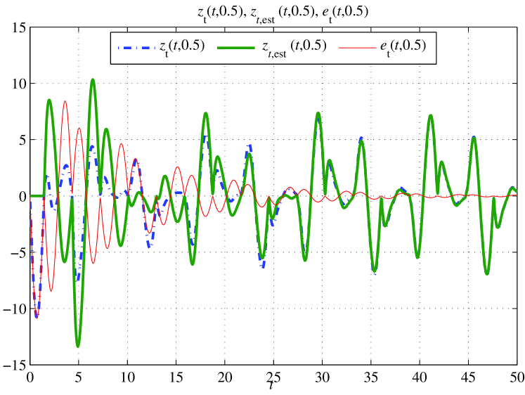
Figure 5: Process of $z_{t}(t,x)$ estimation for $x=0.5$. $z_{t}(t,0.5)$ and $\hat{z}_{t}(t,0.5)$ time histories.

The closed-loop plant-observer-controller (2)–(4), (7)–(9), (10) system behavior is illustrated by Figs. 6 and 7. Control action $u(t)$ time history is shown in Fig. 6 (upper plot), system’s energy $H(t)$ and energy estimate $\widehat{H}(t)$ time histories are demonstrated in Fig. 6 (lower plot). As is seen from the $H(t)$ time history, it achieves the prescribed reference value $H^{*}=10$ simultaneously with vanishing of the energy estimation error $H(t)-\widehat{H}(t)$, and the transient time is about $40$ time units, which is close to that of the observer.

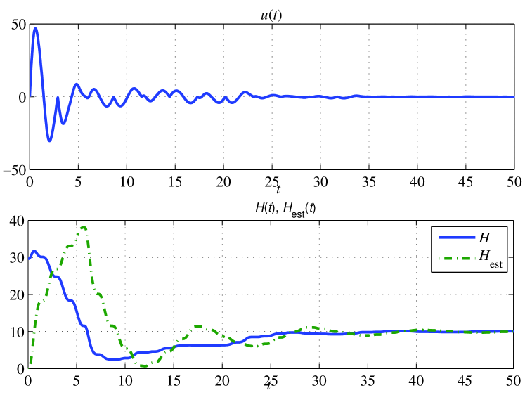
Figure 6: Control action $u(t)$ (upper plot), system’s energy $H(t)$ and energy estimate $\widehat{H}(t)$ (lower plot) time histories.

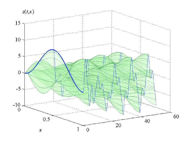
Figure 7: The spatial-temporal plot of $z(t,x)$.

6 Conclusions

In this paper the problem of observer-based boundary control of the sine-Gordon model energy is posed for the first time. A Luenberger-type observer for the sine-Gordon equation is analysed, and explicit inequalities on equation’s parameters ensuring the exponential decay of the estimation error are obtained. With the use of this observer a speed-gradient control law for solving the energy control problem is proposed. Under the assumption that system’s energy does not vanish in finite time the achievement of the control goal is proved. The results of numerical experiments demonstrate that the transient time in energy is close to the transient time in observation error, i.e. the closed-loop system has a reasonable performance.

References

References

- [1] J. Cuevas-Maraver, P. Kevrekidis, F. Williams (Eds.), The sine-Gordon Model and its Applications. From Pendula and Josephson Junctions to Gravity and High-energy Physics, Springer International Publishing, Cham, 2014.
- [2] C. Fuller, S. Elliot, P. Nelson, Active Control of Vibration, Academic Press, London, 1996.
- [3] E. Zuazua, Uniform stabilization of the wave equation by nonlinear boundary feedback, SIAM J. Control Optim. 28 (2) (1990) 466–477.
- [4] I. Lasiecka, R. Triggiani, Uniform stabilization of the wave equation with Dirichlet or Neumann feedback control without geometric conditions, Appl. Math. Optim. 25 (1992) 189–224.
- [5] O. Morgul, A dynamic control law for the wave-equation, Automatica 30 (11) (1994) 1785–1792.
- [6] F. Tröltzsch, Optimal Control of Partial Differential Equations: Theory, Methods and Applications, American Mathematical Society, Providence, 2010.
- [7] P. Christofides, Nonlinear and Robust Control of PDE Systems, Birkhäuser, Boston, 2001.
- [8] A. Smyshlyaev, M. Krstic, Adaptive Control of PDEs, Princeton University Press, Princeton, 2010.
- [9] M. Krstic, A. Smyshlyaev, Boundary control of PDEs: A course on backstepping designs, SIAM, Philadelphia, 2008.
- [10] T. Yang, L. Chua, Impulsive stabilization for control and synchronization of chaotic systems: Theory and application to secure communication, IEEE Trans. Circuits Syst. 44 (10) (1997) 976–988.
- [11] A. Fradkov, A. Pogromsky, Introduction to control of oscillations and chaos, World Scientific Publishers, Singapore, 1998.
- [12] A. Pikovsky, M. Rosenblum, J. Kurths, Synchronization: A Universal Concept in Nonlinear Sciences, Cambridge University Press, New York, 2001.
- [13] A. Fradkov, Swinging control of nonlinear oscillations, Intern. J. Control 64 (1996) 1189–1202.
- [14] A. Shiriaev, A. Fradkov, Stabilization of invariant sets for nonlinear non-affine systems, Automatica 36 (11) (2000) 1709–1715.
- [15] A. Porubov, A. L. Fradkov, B. Andrievsky, Feedback control for some solutions of the sine-Gordon equation, Applied Mathematics and Computation 269 (2015) 17–22.
- [16] Y. Orlov, A. L. Fradkov, B. Andrievsky, Energy control of distributed parameter systems via speed-gradient method: Case study of string and sine-Gordon benchmark models, Intern. J. of Control 90 (11) (2017) 2554–2566.
- [17] T. Kobayashi, Boundary feedback stabilization of the sine-Gordon equation without velocity feedback, J. Sound and Vibration 266 (2003) 775–784.
- [18] M. Petcu, R. Temam, Control for the sine-Gordon equation, ESAIM-Control Optimisation And Calculus Of Variations 10 (4) (2004) 553–573.
- [19] T. Kobayashi, Adaptive stabilization of the sine-Gordon equation by boundary control, Mathematical Methods in the Applied Sciences 27 (8) (2004) 957–970.
- [20] M. Dolgopolik, A. L. Fradkov, B. Andrievsky, Boundary energy control of the sine-Gordon equation, IFAC-PapersOnLine 48 (14) (2016) 148–153.
- [21] E. Fridman, M. Terushkin, New stability and exact observability conditions for semilinear wave equations, Automatica 63 (2016) 1–10.
- [22] A. Pazy, Semigroups of Linear Operators and Applications to Partial Differential Equations, Springer-Verlag, New York, 1983.
- [23] G. H. Hardy, J. E. Littlewood, G. Pólya, Inequalities, Cambridge University Press, Cambridge, 1952.
- [24] J. R. Dormand, P. J. Prince, A family of embedded Runge-Kutta formulae, J. Comp. Appl. Math. 6 (1980) 19–26.