Abstract

We consider the problem of the annual mean temperature prediction. The years taken into account and the corresponding annual mean temperatures are denoted by $0,\ldots,n$ and $t_{0}$, $\ldots$, $t_{n}$, respectively. We propose to predict the temperature $t_{n+1}$ using the data $t_{0}$, $\ldots$, $t_{n}$. For each $0\leq l\leq n$ and each parametrization $\Theta^{(l)}$ of the Euclidean space $\mathbb{R}^{l+1}$ we construct a list of weights for the data $\{t_{0},\ldots,t_{l}\}$ based on the rows of $\Theta^{(l)}$ which are correlated with the constant trend. Using these weights we define a list of predictors of $t_{l+1}$ from the data $t_{0}$, $\ldots$, $t_{l}$. We analyse how the parametrization affects the prediction, and provide three optimality criteria for the selection of weights and parametrization. We illustrate our results for the annual mean temperature of France and Morocco.

Keyword: Parametrization, basis, cubic spline, climate change detection.

1 Motivation

We consider the problem of the annual mean temperature prediction. The years taken into account and the corresponding annual mean temperatures are denoted by $0,\ldots,n$ and $t_{0}$, $\ldots$, $t_{n}$, respectively. We model the behavior of the temperature $i\to t_{i}:=s(i)$ by the column vector $\mathbf{s}^{(n)}=(s(0),\ldots,s(n))^{\top}\in\mathbb{R}^{n+1}$. The aim is to predict the temperature $s(n+1)$ at the year $n+1$.

For each $0\leq l\leq n$ and each parametrization $\Theta^{(l)}=(\theta_{ji}^{(l)}:\quad i,j=0,\ldots,l)$ of the Euclidean space $\mathbb{R}^{l+1}$ we construct a list of weights for the data $\{t_{0},\ldots,t_{l}\}$ based on the row $\theta_{j}^{(l)}$ of $\Theta^{(l)}$ which is correlated with the constant trend $\{{\bf 1}^{(l)}\}^{\top}=(1,\ldots,1)$, i.e., $\theta_{j}^{(l)}{\bf 1}^{(l)}\neq 0$. We analyze how the parametrization $\Theta^{(l)}$ affects the prediction. We also propose a list of criteria for selecting optimal parametrization and weights. We illustrate our results for the annual mean temperature of France and Morocco.

The present paper is the first part of a list of works in preparation. These works are directly related to [5], [6] and [7], see also [3], [4], [8].

2 Parametrization

Let $0\leq l\leq n$ be an integer and $\Theta^{(l)}$ be any invertible $(l+1)\times(l+1)$ real matrix. Its $j$-th row is denoted by $\theta_{j}^{(l)}$ and then its entry $(j,i)$ is equal to $\theta_{ji}^{(l)}$, with $i,j=0,\ldots,l$. Its inverse $\{\Theta^{(l)}\}^{-1}$ is denoted by $\mathbf{B}^{(l)}$. The $j$-th column of $\mathbf{B}^{(l)}$ is denoted by $\mathbf{b}_{j}^{(l)}$ and then its entry $(i,j)$ is equal to $b_{ij}^{(l)}$. Let $\mathbf{s}^{(l)}=(s(0),\ldots,s(l))^{\top}\in\mathbb{R}^{l+1}$ be any column vector. The equality

$$\mathbf{s}^{(l)}=\mathbf{B}^{(l)}\Theta^{(l)}\mathbf{s}^{(l)}$$

tells us that

$$\mathbf{s}^{(l)}=\sum_{j=0}^{l}\theta_{j}^{(l)}\mathbf{s}^{(l)}\,\mathbf{b}_{j}^{(l)}.$$ (2.1)

Hence the columns $[\mathbf{b}_{0}^{(l)},\ldots,\mathbf{b}_{l}^{(l)}]$ of the matrix $\mathbf{B}^{(l)}$ form a basis of $\mathbb{R}^{l+1}$, and $(\theta_{0}^{(l)}\mathbf{s}^{(l)},\ldots,\theta_{l}^{(l)}\mathbf{s}^{(l)})$ are the coordinates of the vector $\mathbf{s}^{(l)}$ in the basis $\mathbf{B}^{(l)}$.

Proposition 2.1.

Let ${\bf 1}^{(l)}=(1,\ldots,1)^{\top}\in\mathbb{R}^{l+1}$ denotes the constant trend written as column vector, and $I(l)=\{j:\quad\theta_{j}^{(l)}{\bf 1}^{(l)}\neq 0\}$. We have for $i=0,\ldots,l$,

$$\sum_{j\in I(l)}\theta_{j}^{(l)}{\bf 1}^{(l)}b_{ij}^{(l)}=1,$$

$$s(i)=\sum_{j\in I(l)}\theta_{j}^{(l)}\mathbf{s}^{(l)}\,b_{ij}^{(l)}+\sum_{j\notin I(l)}\theta_{j}^{(l)}\mathbf{s}^{(l)}\,b_{ij}^{(l)}.$$

Proof.

It is the consequence of the equality

$$1=\sum_{j=0}^{l}\theta_{j}^{(l)}{\bf 1}^{(l)}\,b_{ij}^{(l)}$$

$$=\sum_{j\in I(l)}\theta_{j}^{(l)}{\bf 1}^{(l)}\,b_{ij}^{(l)},$$

with $i=0,\ldots,l$. ∎

If $s(i)$ oscillates around some constant $c$, then $\sum_{j\notin I(l)}\theta_{j}^{(l)}\mathbf{s}^{(l)}\,b_{ij}^{(l)}$ oscillates around 0. Hence the component $\sum_{j\in I(l)}\theta_{j}^{(l)}\mathbf{s}^{(l)}\,b_{ij}^{(l)}$ seems to be the bulk component of $s(i)$, and $\sum_{j\notin I(l)}\theta_{j}^{(l)}\mathbf{s}^{(l)}\,b_{ij}^{(l)}$ its residual component. Roughly speaking, the most important coordinates are those correlated with the constant trend ${\bf 1}^{(l)}$, i.e., $(\theta_{j}^{(l)}:\quad j\in I(l))$.

3 Conservative rows and selection criteria

3.1 Conservative rows

The row $\mathbf{p}=(p_{0},\ldots,p_{l})\in\mathbb{R}^{l+1}$ is conservative if

$$\sum_{i=0}^{l}p_{i}=1.$$

If $p_{i}\geq 0$ for all $i$, then $\mathbf{p}$ is a probability distribution on the set $\{0,\ldots,l\}$. The set of conservative rows is denoted by

$$M_{1}(\{0,\ldots,l\})=\{\mathbf{p}\in\mathbb{R}^{l+1}:\quad\sum_{i=0}^{l}p_{i}=1\}.$$

The mean and the variance of $\mathbf{s}^{(l)}$ w.r.t. to $\mathbf{p}$ are defined respectively by

$$m_{1}(\mathbf{p})=\mathbf{p}\mathbf{s}^{(l)}=\sum_{i=0}^{l}p_{i}s(i),$$

$$\mbox{var}(\mathbf{p})=\sum_{i=0}^{l}p_{i}|s(i)-m_{1}(\mathbf{p})|^{2}.$$

We have the famous equality

$$\sum_{i=0}^{l}p_{i}x_{i}^{2}=m_{1}^{2}(\mathbf{p})+\mbox{var}(\mathbf{p}).$$

Observe also as in the probabilistic case, the minimizer

$$\arg\min\{\sum_{i=0}^{l}p_{i}|s(i)-a|^{2}:\quad a\in\mathbb{R}\}=m_{1}(\mathbf{p}),$$

and the error

$$\min\{\sum_{i=0}^{l}p_{i}|s(i)-a|^{2}:\quad a\in\mathbb{R}\}=\mbox{var}(\mathbf{p}).$$

3.2 Selection criterion

The set $\mathcal{P}$ contains a finite number of parametrizations of the Euclidean spaces $(\mathbb{R}^{2},\ldots,\mathbb{R}^{n+1})$. An element of $\mathcal{P}$ is a parametrization $\Theta:=(\Theta^{(1)},\ldots,\Theta^{(n)})$ of the Euclidean spaces $(\mathbb{R}^{2},\ldots,\mathbb{R}^{n+1})$.

Let us give for each $1\leq l\leq n$ and each parametrization $\Theta^{(l)}$ a finite subset $W(\Theta^{(l)})$ of the set of conservative rows $M_{1}(\{0,\ldots,l\})$. We get the subset $W(\Theta):=W(\Theta^{(1)})\times\ldots\times W(\Theta^{(n)})$ of $M_{1}(\{0,1\})\times\ldots\times M_{1}(\{0,\ldots,n\})$.

A selection criterion $S$ picks a unique element

$$SW(\Theta)=(SW(\Theta^{(1)}),\ldots,SW(\Theta^{(n)}))\in M_{1}(\{0,1\})\times\ldots\times M_{1}(\{0,\ldots,n\})$$

from the set $W(\Theta)$.

3.3 Prediction cost

We propose for each $l=1,\ldots,n$,

$$SW(\Theta^{(l)})\mathbf{s}^{(l)}$$

as a prediction of $s(l+1)$. The cost of these predictors for $q=1,2,+\infty$, and $L<n$ fixed, is measured by

$$\mbox{Cost}(SW(\Theta),q)=\frac{\sum_{l=L}^{n-1}|s(l+1)-SW(\Theta^{(l)})\mathbf{s}^{(l)}|^{q}}{n-L},\quad q=1,2,$$

$$:=\max\{|s(l+1)-SW(\Theta^{(l)})\mathbf{s}^{(l)}|:\quad L\leq l\leq n-1\},\quad q=+\infty.$$

Let $\mathcal{S}$ be a finite set of selection criteria. The optimal selection criterion $S^{*}W(\Theta^{*},q)$ is the minimizer

$$S^{*}W(\Theta^{*},q)=\arg\min\{\mbox{Cost}(SW(\Theta),q):\quad\Theta\in\mathcal{P},\quad S\in\mathcal{S}\}.$$

In this work we consider the sets

$$W(\Theta^{(l)})=\left\{\frac{\theta_{j}^{(l)}}{\theta_{j}^{(l)}{\bf 1}^{(l)}}:\,\,0\leq j\leq l,\,\,\theta_{j}^{(l)}{\bf 1}^{(l)}\neq 0\right\},$$

with $l=1,\ldots,n$. We recall that $I(l)=\{0\leq j\leq l:\quad\theta_{j}^{(l)}{\bf 1}^{(l)}\neq 0\}$. Observe that for each parametrization $\Theta^{(l)}$, the set $I(l)$ is not empty.

For simplicity we denote for each selection criterion $S$

$$S(\Theta^{(l)}):=SW(\Theta^{(l)}),\quad l=1,\ldots,n.$$

Now, we are going to define our selection criteria.

3.4 The selection criterion $S_{u}$

Let $I(l)=\{j(0),\ldots,j(card(I(l))-1)\}$ be the elements of the set $I(l)$ with $j(0)<\ldots<j(card(I(l))-1)$. We define for each $u\leq n$ fixed the selection criterion

$$S_{u}(\Theta^{(l)})=\frac{\theta_{j(\min(u,card(I(l))-1))}^{(l)}}{\theta_{j(\min(u,card(I(l))-1))}^{(l)}{\bf 1}^{(l)}}.$$

If $u=0$, then

$$S_{0}(\Theta^{(l)})=\frac{\theta_{j(0)}^{(l)}}{\theta_{j(0)}^{(l)}{\bf 1}^{(l)}}.$$

If $u=n$, then

$$S_{n}(\Theta^{(l)})=\frac{\theta_{j(card(I(l))-1)}^{(l)}}{\theta_{j(card(I(l))-1)}^{(l)}{\bf 1}^{(l)}}.$$

3.5 The winning conservative rows $S_{u(q,\Theta)}(\Theta)$

Given $\Theta$ and $q=1,2,+\infty$, the optimal selection criterion among $(S_{u}:\quad u=0,\ldots,n)$ is given by the minimizer

$$u(q,\Theta)=\arg\min\{\mbox{Cost}(S_{u}(\Theta),q):\quad u=0,\ldots,n\}.$$

Hence $S_{u(q,\Theta)}(\Theta)$ is the optimal conservative rows among the set $(S_{u}(\Theta):\quad u=0,\ldots,n)$ of conservative rows.

3.6 The selection criterion $S_{\mbox{\small{mean}}}$

For $1\leq l\leq n$, we consider the selection criterion

$$S_{\mbox{\small{mean}}}(\Theta^{(l)})=\sum_{j\in I(l)}\frac{\theta_{j}^{(l)}}{card(I(l))\theta_{j}^{(l)}{\bf 1}^{(l)}}.$$

Observe that for the canonical parametrization $\Theta^{(l)}=(\delta_{i}^{j}:0\leq i,j\leq l)$, we have

$$S_{\small{\mbox{\small{mean}}}}(\Theta^{(l)})=(\frac{1}{l+1},\ldots,\frac{1}{l+1}).$$

3.7 The winning conservative rows $S_{1,q}(\Theta)$

Given $\Theta$ and $q=1,2,+\infty$, the optimal conservative rows among $S_{u(q,\Theta)}(\Theta)$ and $S_{\mbox{\small{mean}}}(\Theta)$ is the minimizer

$$S_{1,q}(\Theta):=\arg\min\{\mbox{Cost}(S_{u(q,\Theta)}(\Theta),q),\mbox{Cost}(S_{\mbox{\small{mean}}}(\Theta),q)\}.$$

3.8 The selection criterion $S_{u\mbox{\small{tail1}}}$

For a fixed $u\leq n$ the set

$$J_{1}(l,u)=\arg\max\{\sum_{i=\min(u,l)}^{l}\frac{\theta_{ji}^{(l)}}{\theta_{j}^{(l)}{\bf 1}^{(l)}}:\quad j\in I(l)\}$$

may be not a singleton. It furnishes the selection criterion

$$S_{\mbox{\small{tail1}}}(\Theta^{(l)})=\sum_{j\in J_{1}(l,u)}\frac{\theta_{j}^{(l)}}{card(J_{1}(l,u))\theta_{j}^{(l)}{\bf 1}^{(l)}}.$$

As a simple example, if $\Theta^{(l)}$ is the canonical parametrization and $u=n$, then

$$J_{1}(l,n)=l.$$

If $u=n-1$, then $J_{1}(l,n-1)=l$ for $l\leq n-1$, and $J_{1}(n,n-1)=\{n-1,n\}$.

3.9 The winning conservative rows $S_{u(q,\Theta)\mbox{\small{tail1}}}(\Theta)$

The optimal selection criterion among $(S_{u\mbox{\small{tail1}}}:\quad u=0,\ldots,n)$ is the minimizer of

$$S_{u(q,\Theta)\mbox{\small{tail1}}}=\arg\min\{\mbox{Cost}(\Theta,S_{u\mbox{\small{tail1}}}(\Theta),q):\quad u=0,\ldots,n\}.$$

3.10 The winning conservative rows $S_{2,q}(\Theta)$

The winner for each $q=1,2,+\infty$ fixed, among $S_{u(q,\Theta)\mbox{\small{tail1}}}(\Theta)$ and $S_{1,q}(\Theta)$ is the minimizer

$$S_{2,q}(\Theta):=\arg\min\{\mbox{Cost}(S_{u(q,\Theta)\mbox{\small{tail1}}}(\Theta),q),\mbox{Cost}(S_{1,q}(\Theta),q)\}.$$

3.11 The selection criterion $S_{u\mbox{\small{tail2}}}$

For a fixed $u\leq n$ the set

$$J_{2}(l,u)=\arg\max\{\max\{\frac{\theta_{ji}^{(l)}}{\theta_{j}^{(l)}{\bf 1}^{(l)}}:\quad\min(u,l)\leq i\leq l\}:\quad j\in I(l)\},$$

may be not a singleton. It furnishes the selection criterion

$$S_{\mbox{\small{tail2}}}(\Theta^{(l)})=\sum_{j\in J_{2}(l,u)}\frac{\theta_{j}^{(l)}}{card(J_{2}(l,u))\theta_{j}^{(l)}{\bf 1}^{(l)}}.$$

3.12 The winning conservative rows $S_{u(q,\Theta)\mbox{\small{tail2}}}(\Theta)$

The optimal selection criterion among $(S_{u\mbox{\small{tail2}}}:\quad u=0,\ldots,n)$ is the minimizer of

$$S_{u(q,\Theta)\mbox{\small{tail2}}}=\arg\min\{\mbox{Cost}(S_{u\mbox{\small{tail2}}}(\Theta),q):\quad u=0,\ldots,n\}.$$

3.13 The winning conservative rows $S_{3,q}(\Theta)$

The winner for each $q=1,2,+\infty$ fixed, among $S_{u(q,\Theta)\mbox{\small{tail2}}}(\Theta)$ and $S_{2,q}(\Theta)$ is the minimizer

$$S_{3,q}(\Theta):=\arg\min\{\mbox{Cost}(S_{u(q,\Theta)\mbox{\small{tail2}}}(\Theta),q),\mbox{Cost}(S_{2,q}(\Theta),q)\}.$$

3.14 The selection criterion $S_{\small{maxcor}}$

The set

$$J_{3}(l)=\arg\max\{\frac{|\theta_{j}^{(l)}{\bf 1}^{(l)}|}{\sqrt{l+1}\|\theta_{j}^{(l)}\|}:\quad j\in I(l)\}$$

of the coordinates $\theta_{j}^{(l)}$ highly correlated with the constant trend ${\bf 1}^{(l)}$, furnishes the selection criterion

$$S_{\mbox{\small{maxcor}}}(\Theta^{(l)})=\sum_{j\in J_{3}(l)}\frac{\theta_{j}^{(l)}}{card(J_{3}(l))\theta_{j}^{(l)}{\bf 1}^{(l)}}.$$

3.15 The winning conservative rows $S_{4,q}(\Theta)$

The winner for each $q=1,2,+\infty$ fixed, among $S_{\mbox{maxcor}}(\Theta)$ and $S_{3,q}(\Theta)$ is the minimizer

$$S_{4,q}(\Theta):=\arg\min\{\mbox{Cost}(S_{\mbox{maxcor}}(\Theta),q),\mbox{Cost}(S_{3,q}(\Theta),q)\}.$$

3.16 The selection criterion $S_{q\mbox{\small{nearU}}}$

We consider the set

$$J_{4}(l,q)=\arg\min\{\|\frac{\theta_{j}^{(l)}}{\theta_{j}^{(1)}{\bf 1}^{(l)}}-(\frac{1}{l+1},\ldots,\frac{1}{l+1})\|_{q}:\quad j\in I(l)\}$$

of the nearest conservative rows $\frac{\theta_{j}^{(l)}}{\theta_{j}^{(1)}{\bf 1}^{(l)}}$ to the uniform conservative row $(\frac{1}{l+1},\ldots,\frac{1}{l+1})$, and the corresponding selection criterion

$$S_{q\mbox{\small{nearU}}}(\Theta^{(l)})=\sum_{j\in J_{4}(l,q)}\frac{\theta_{j}^{(l)}}{card(J_{4}(l,q))\theta_{j}^{(l)}{\bf 1}^{(l)}}.$$

Here $\|\cdot\|_{q}$ denotes the $l(q)$-norm with $q=1,2,+\infty$.

3.17 The winning conservative rows $S_{q(\Theta)\mbox{\small{nearU}}}(\Theta)$

For each $q=1,2,+\infty$ fixed let us denote by

$$q(\Theta)=\arg\min\{\mbox{Cost}(S_{q_{1}\mbox{\small{nearU}}}(\Theta),q):\quad q_{1}=1,2,+\infty\},$$

and then we obtain the winning conservative rows $S_{q(\Theta)\mbox{\small{nearU}}}(\Theta)$ among the three conservative rows $(S_{q_{1}\mbox{\small{nearU}}}(\Theta):\quad q_{1}=1,2,+\infty)$.

3.18 The winning conservative rows $S_{5,q}(\Theta)$

For each $q=1,2,+\infty$ fixed, the winner among $S_{q(\Theta)\mbox{\small{nearU}}}(\Theta)$ and $S_{4,q}(\Theta)$ is the minimizer

$$S_{5,q}(\Theta):=\arg\min\{\mbox{Cost}(S_{q(\Theta)\mbox{\small{nearU}}}(\Theta),q),\mbox{Cost}(S_{4,q}(\Theta),q)\}.$$

3.19 The selection criterion $S_{u\mbox{\small{var}}}$

For each $j\in I(l)$ the variance of the data $\mathbf{s}^{(l)}$ w.r.t. to the conservative row $\frac{\theta_{j}^{(l)}}{\theta_{j}^{(l)}{\bf 1}^{(l)}}$ is denoted by $var(l,j)$. We define the one-to-one map $\sigma^{(l)}$ from $\{0,\ldots,card(I(l))-1\}$ to $I(l)$ as follows. The integer $\sigma^{(l)}(0)$ is the first element of

$$\arg\min\{\mbox{var}(l,j):\quad j\in I(l)\}.$$

By induction for $k<card(I(l))-1$ the integer $\sigma^{(l)}(k+1)$ is the first element of

$$\arg\min\{\mbox{var}(l,j):\quad j\in I(l)\setminus\{\sigma^{(l)}(0),\ldots,\sigma^{(l)}(k)\}\}.$$

We define for a fixed $u\leq n$ the index

$$j(l,u)=\sigma^{(l)}(\min(u,card(I(l))-1)),$$

and the selection criterion

$$S_{u\mbox{\small{var}}}(\Theta^{(l)})=\frac{\theta_{j(l,u)}^{(l)}}{\theta_{j(l,u)}^{(l)}{\bf 1}^{(l)}}.$$

If $u=n$, then $j(l,n)=\sigma^{(l)}(card(I(l))-1)$ is the index of the largest variance. If $u=0$, then $j(l,0)=\sigma^{(l)}(0)$ is the index of the smallest variance.

3.20 The winning conservative rows $S_{u(q,\Theta)\mbox{\small{var}}}(\Theta)$

The optimal selection criterion among $(S_{u\mbox{\small{var}}}:\quad u=0,\ldots,n)$ is the minimizer of

$$S_{u(q,\Theta)\mbox{\small{var}}}=\arg\min\{\mbox{Cost}(\Theta,S_{u\mbox{\small{var}}}(\Theta),q):\quad u=0,\ldots,n\}.$$

3.21 The winning conservative sequence $S_{6,q}(\Theta)$

The winner for each $q=1,2,+\infty$ fixed, among $S_{u(q,\Theta)\mbox{\small{var}}}(\Theta)$ and $S_{5,q}(\Theta)$ is the minimizer

$$S_{6,q}(\Theta):=\arg\min\{\mbox{Cost}(\Theta,S_{u(q,\Theta)\mbox{\small{var}}}(\Theta),q),\mbox{Cost}(\Theta,S_{5,q}(\Theta),q)\}.$$

3.22 The selection criterion $S_{uv\small{fd}}$

We define for each fixed $\tilde{l}\leq l$ the permutation $\sigma^{(l,\tilde{l})}$ of the set $I(l)$ as follows. The integer $\sigma^{(l,\tilde{l})}(0)$ is the first element of

$$\arg\min\{|\frac{\theta_{j}^{(l)}\mathbf{s}^{(l)}}{\theta_{j}^{(l)}{\bf 1}^{(l)}}-s(\tilde{l})|:\quad j\in I(l)\}.$$

By induction for $k<card(I(l))-1$, $\sigma^{(l,\tilde{l})}(k+1)$ is the first element of

$$\arg\min\{|\frac{\theta_{j}^{(l)}\mathbf{s}^{(l)}}{\theta_{j}^{(l)}{\bf 1}^{(l)}}-s(\tilde{l})|:\quad j\in I(l)\setminus\{\sigma^{(l,\tilde{l})}(0),\ldots,\sigma^{(l,\tilde{l})}(k)\}\}.$$

Let $0\leq u\leq n$, $0\leq v\leq n$ fixed. The selection criterion

$$j(l,u,v)=\sigma^{(l,\min(l,u))}(\min(v,card(I(l))-1))$$

furnishes the selection criterion

$$S_{uvfd}(\Theta)=\frac{\theta_{j(l,u,v)}^{(l)}}{\theta_{j(l,u,v)}^{(l)}{\bf 1}^{(l)}}.$$

If $u=v=n$, then $j(l,n,n)=\sigma^{(l,l)}(card(I(l))-1)$ is the index of the farest element $\frac{\theta_{j}^{(l)}\mathbf{s}^{(l)}}{\theta_{j}^{(l)}{\bf 1}^{(l)}}$ from $s(l)$. If $u=0,v=n$, then $j(l,0,n)=\sigma^{(l,0)}(card(I(l))-1)$ is the index of the farest element $\frac{\theta_{j}^{(l)}\mathbf{s}^{(l)}}{\theta_{j}^{(l)}{\bf 1}^{(l)}}$ from $s(0)$. If $u=v=0$, then $j(l,0,0)=\sigma^{(l,0)}(0)$ is the index of the nearest element $\frac{\theta_{j}^{(l)}\mathbf{s}^{(l)}}{\theta_{j}^{(l)}{\bf 1}^{(l)}}$ from $s(0)$.

3.23 The winning conservative rows $S_{u(q,\Theta)v(q,\Theta)\small{fd}}(\Theta)$

Given $\Theta$ and $q=1,2,+\infty$, the optimal conservatrice sequence $S_{u(q,\Theta)v(q,\Theta)\small{fd}}(\Theta)$ among $(S_{uv\small{fd}}(\Theta):\quad u,v=0,\ldots,n)$ is given by the minimizer

$$(u(q,\Theta),v(q,\Theta))=\arg\min\{\mbox{Cost}(S_{uv\small{fd}}(\Theta),q):\quad u,v=0,\ldots,n\}.$$

3.24 The winning conservative rows $S_{7,q}(\Theta)$

Given $\Theta$ and $q=1,2,+\infty$, the optimal conservative rows $S_{7,q}(\Theta)$ among $S_{u(q,\Theta)v(q,\Theta)\mbox{fd}}(\Theta)$ and $S_{6,q}(\Theta)$ is the minimizer

$$\arg\min\{\mbox{Cost}(S_{u(q,\Theta)v(q,\Theta)\mbox{fd}}(\Theta),q,L),\mbox{Cost}(S_{6,q}(\Theta),q)\}.$$

4 The winning conservative rows $S_{7}(\Theta(q))$

We constructed for $q=1,2,+\infty$ fixed and each parametrization $\Theta$ the optimal conservative rows $S_{7,q}(\Theta)$. Assume that we have a finite set $\mathcal{P}$ of parametrizations. The minimizer $\Theta^{*}(q)$ of the map

$$\Theta\to\mbox{Cost}(S_{7,q}(\Theta),q)$$

furnishes the optimal selection criterion $S_{7}(\Theta(q)):=S_{7,q}(\Theta(q))$.

5 Application to parametrizations given by the energy of the spline

We identify for the integer $l\geq 1$ the space $\mathbb{R}^{l+1}$ with the space of the natural cubic splines $S_{3,nat}(0,\ldots,l)$ having the knots $0,\ldots,l$. Let us denote $S_{3}(0,\ldots,l)$ the set of cubic splines having the knots $0,\ldots,l$. We recall that an element $s\in S_{3}$ is a $C^{2}$ map on $[0,l]$ and is a polynomial of degree three on each interval $[i,i+1)$ for $i=0$,…, $l-1$. More precisely, let

$$p_{0}=s(0),\ldots,p_{l}=s(l),\quad q_{0}=s^{\prime}(0),\ldots,q_{l}=s^{\prime}(l),$$

$$u_{0}=s^{\prime\prime}(0),\ldots,u_{l}=s^{\prime\prime}(l),\quad v_{0}=s^{\prime\prime\prime}(0+),\ldots,v_{l-1}=s^{\prime\prime\prime}(l-1+)$$

be respectively the values of $s$ and its derivatives up to order three on the knots. We have for $i=0,\ldots,l-1$,

$$s(t)=p_{i}+q_{i}(t-i)+(t-i)^{2}u_{i}/2+(t-i)^{3}v_{i}/6,\quad t\in[i,i+1).$$

The following constraint guarantees the hypothesis that $s$ is $C^{2}$:

$$p_{i}+q_{i}+u_{i}/2+v_{i}/6=p_{i+1},\quad$$ (5.1)

$$q_{i}+u_{i}+v_{i}/2=q_{i+1},\quad$$ (5.2)

$$v_{i}=s^{(3)}(t_{i})=u_{i+1}-u_{i}.\quad$$ (5.3)

It is well known [2] that $S_{3}(0,\ldots,l)$ has the dimension $l+3$, see also [1] and [9]. Hence an element $s\in S_{3}(0,\ldots,l)$ is completely defined by $l+3$ independent parameters. Moreover, the set of natural cubic splines $S_{3,nat}(0,\ldots,l)$ is the set of cubic spline $s$ with $s^{\prime\prime}(0)=s^{\prime\prime}(l)=0$. Hence the dimension of $S_{3,nat}(0,\ldots,l)$ is equal to $l+1$. Now we are ready to define our parametrizations of $\mathbb{R}^{l+1}$.

There exist for each $l$ fixed a unique non symmetric matrix $\mathbf{M}^{(l)}$ and a unique symmetric matrix $\mathbf{S}^{(l)}$ such that

$$\int_{0}^{l}|s(t)|^{2}dt=\{\mathbf{s}^{(l)}\}^{\top}\mathbf{M}^{(l)}\mathbf{s}^{(l)}=\{\mathbf{s}^{(l)}\}^{\top}\mathbf{S}^{(l)}\mathbf{s}^{(l)},$$

for all $s\in S_{3,nat}(0,\ldots,l)$.

We consider the following six parametrization matrices $\Theta^{(l)}=\mathbf{M}^{(l)}$, $\{\mathbf{M}^{(l)}\}^{\top}$, $\{\mathbf{M}^{(l)}\}^{-1}$, $\{\{\mathbf{M}^{(l)}\}^{-1}\}^{\top}$, $\mathbf{S}^{(l)}$, $\{\mathbf{S}^{(l)}\}^{-1}$.

Figure 1: Represantation of the basis $\mathbf{B}^{(l)}=\mathbf{M}^{(l)}$ with $l=7$.

Figure 2: Representation of the basis $\mathbf{B}^{(l)}=\mathbf{S}^{(l)}$ with $l=7$.

5.1 Real data application

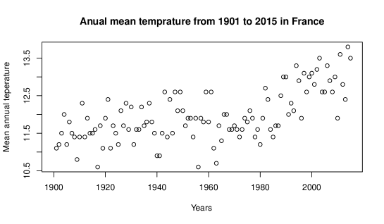
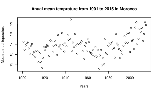
In the temperature prediction problem we are interested in the annual mean temperature observed in France and Morocco from 1901 to 2015. Data $\mathbf{s}^{(n)}=(s(0),\ldots,s(n))^{\top}$ with $n=114$ respectively for France and Morocco are presented in Figure(3). Observe that $s(n)$ denotes the temperature of the year $n+1$.

Figure 3: Annual mean temperatures in France and Morocco from 1901 to 2015

5.1.1 Predictors

Our set of parametrizations $\mathcal{P}$ contains

$$\mathbf{M}=(\mathbf{M}^{(l)}:\quad l=1,\ldots,n),$$

$$\mathbf{M}^{\top}=(\{\mathbf{M}^{(l)}\}^{\top}:\quad l=1,\ldots,n),$$

$$\mathbf{M}^{-1}=(\{\mathbf{M}^{(l)}\}^{-1}:\quad l=1,\ldots,n),$$

$$\{\mathbf{M}^{-1}\}^{\top}=(\{\{\mathbf{M}^{(l)}\}^{-1}\}^{\top}:\quad l=1,\ldots,n),$$

$$\mathbf{S}=(\mathbf{S}^{(l)}:\quad l=1,\ldots,n),$$

$$\mathbf{S}^{-1}=(\{\mathbf{S}^{(l)}\}^{-1}:\quad l=1,\ldots,n).$$

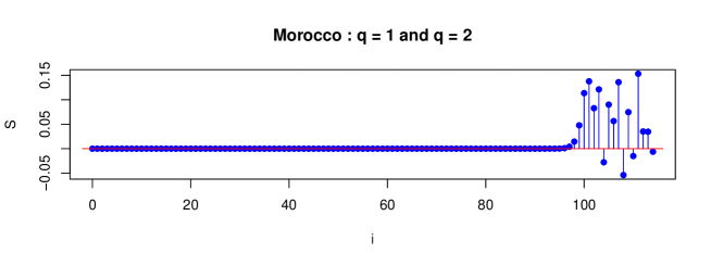
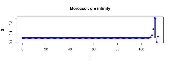
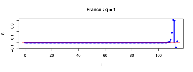
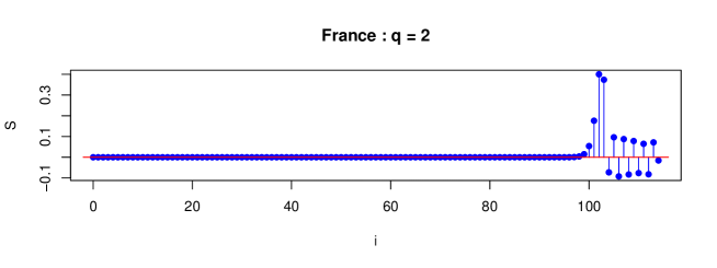
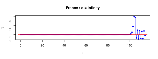
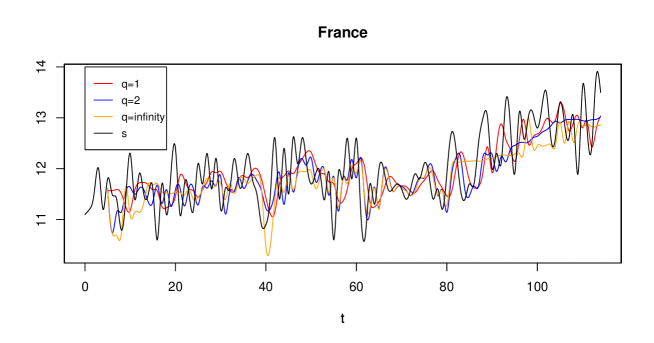
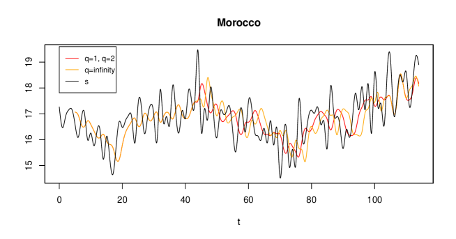
Table (1) shows that for each $q=1,2,+\infty$ and the lag $L=4$ the optimal parametrization $\Theta(q)=\mathbf{M}^{-1}$ for both France and Morocco, but the optimal conservative rows $S_{7}(\Theta(q))$ do not coincide. The optimal conservative rows $S_{7}(\Theta^{(114)}(q))$ are plotted in Figures (4) and (5). The predictors of the temperature $s(114)$ (the temperature at the year 2015) and the true temperature is given in Table (2). The predictors of the temperature $s(115)$ (the temperature at the year 2016) is given in Table (3). Splines of the true temperature and its optimal predictors are represented in Figure (6).

Table 1: The optimal choice $\Theta(q)$ and $S_{7}(\Theta(q))$.

Country	France
$q$	1	2	$\infty$
$\Theta(q)$	$\mathbf{M}^{-1}$	$\mathbf{M}^{-1}$	$\mathbf{M}^{-1}$
$S_{7}(\Theta(q))$	$S_{u\mbox{\small{tail2}}}$ $(u=86)$	$S_{uv\small{fd}}$ $(u=93,v=5)$	$S_{uv\small{fd}}$ $(u=81,v=8)$
cost	0.4233063	0.2784530	1.220770
Country	Morocco
$q$	1	2	$\infty$
$\Theta(q)$	$\mathbf{M}^{-1}$	$\mathbf{M}^{-1}$	$\mathbf{M}^{-1}$
$S_{7}(\Theta(q))$	$S_{u\mbox{\small{tail1}}}$ $(u=73)$		$S_{u\mbox{\small{tail2}}}$ $(u=41)$
cost	0.6183125	0.6027288	1.917094

Table 2: The best prediction of $s(114)$ using the optimal parametrization $\Theta(q)=\mathbf{M}^{-1}$ and the optimal conservative rows $S_{7}(\Theta(q))$.

Country	France
$q$	1	2	$\infty$
True temperature	13.8
Prediction	13.03396	13.01986	12.86248
Country	Morocco
$q$	1	2	$\infty$
True temperature	19.20845
Prediction	18.17489	18.17489	18.06860

Table 3: The best prediction of $s(115)$ (the temperature at the year 2016) using the optimal parametrization $\Theta(q)=\mathbf{M}^{-1}$ and the optimal conservative rows $S_{7}(\Theta(q))$.

Country	France
$q$	1	2	$\infty$
Prediction	12.66792	13.06234	12.82844
Country	Morocco
$q$	1	2	$\infty$
Prediction	17.53958	17.53958	17.76148

Figure 4: The optimal conservative row $S_{7}(\Theta^{(114)}(q))$, $q=1,2,\infty$ for Morocco.

Figure 5: The optimal conservative row $S_{7}(\Theta^{(114)}(q))$, $q=1,2,\infty$ for France.

Figure 6: The splines of $\mathbf{s}^{(n)}$ and its optimal predictors, with $n=114$.

Conclusion. Having a time series $s(0)$, $\ldots$, $s(n)$ with values in $\mathbb{R}$, we showed how to predict the value $s(n+1)$ from each parametrization of the set $\mathbb{R}^{n+1}$. We also provided optimality criteria to select the best predictor. This work can be extended to time series $s(i)\in K$ with $K$ is any field or vector space.

References

• [1] P. Craven, G. Wahba, Smoothing noisy data with spline functions, Numer. Math. 31 (4) (1978) 377–390.
• [2] C. deBoor, A Practical Guide to Spline, Springer (1978) Springer.
• [3] A. Dermoune, B. Djehiche, N. Rahmania, A consistent estimator of the smoothing parameter in the Hodrick-Prescott filter J. Japan Statist. Soc., 38 (2) (2008) 225–241.
• [4] A. Dermoune, B. Djehiche, N. Rahmania, Multivariate Extension of the Hodrick-Prescott Filter- Optimality and Characterization, Studies in NonLinear dynamics and Econometrics, 13 (3) (2009) Article 4.
• [5] A. Dermoune, C. Preda, Estimation of noisy cubic spline using a natural basis, Annals of the University of Craiova, Mathematics and Computer Science Series 43 (1) (2016) 33–52.
• [6] A. Dermoune, C. Preda, Parametrizations, fixed and random effects, Journal of Multivariate Analysis 154 (2017) 162-176.
• [7] A. Dermoune, N. Rahmania, T. Wei, General Linear mixed model and signal extraction problem with constraint, Journal of Multivariate Analysis, 105 (1) (2012) 311–321.
• [8] A. Dermoune, T. Wei, FastICA algorithm: Five criteria for the optimal choice of the nonlinearity function, IEEE transactions on signal processing 61 (8), 2078-2087 (27) 2013.
• [9] G. Wahba, Spline models for observational data. Society for Industrial and Applied Mathematics (SIAM) (1990).