Nonrelativistic hydrodynamics from quantum field theory:

Abstract

We provide a complete derivation of hydrodynamic equations for nonrelativistic systems based on quantum field theories of spinless Schrödeinger fields, assuming that an initial density operator takes a special form of the local Gibbs distribution. The constructed optimized/renormalized perturbation theory for real-time evolution enables us to separately evaluate dissipative and nondissipative parts of constitutive relations. It is shown that the path-integral formula for local thermal equilibrium together with the symmetry properties of the resulting action— the nonrelativistic diffeomorphism and gauge symmetry in the thermally emergent Newton-Cartan geometry—provides a systematic way to derive the nondissipative part of constitutive relations. We further show that dissipative parts are accompanied with the entropy production operator together with two kinds of fluctuation theorems by the use of which we derive the dissipative part of constitutive relations and the second law of thermodynamics. After obtaining the exact expression for constitutive relations, we perform the derivative expansion and derive the first-order hydrodynamic (Navier-Stokes) equation with the Green-Kubo formula for transport coefficients.

1 Introduction and Summary

1.1 Introduction

Hydrodynamics is one of the most established theoretical framework by the use of which we can describe real-time dynamics of many-body systems. To be more precise, hydrodynamics captures the macroscopic spacetime evolution of the conserved charge densities such as the energy and momentum densities Landau:Fluid . One most important feature of hydrodynamics is that it provides universal description of any many-body system: We can apply it to air and water in our daily life, strongly correlated electron systems in condensed matter physics, nuclear matter inside the neutron stars in astrophysics, the quark-gluon plasma in high-energy physics, and also active matters in biological systems. Hydrodynamic analysis including precise numerical simulations is now indispensable tool to investigate real-time dynamics in many fields of science.

Nevertheless, compared to its successful applications, foundation of hydrodynamics based on underlying microscopic theories—in particular, quantum field theories—remains unclear. In fact, although this problem has been pursued for a long time in development of nonequilibrium (classical) statistical mechanics Nakajima ; Mori1 ; McLennan ; McLennan1 ; Zubarev:1979 ; Zubarev1 ; Zubarev2 ; PhysRevA.8.2048 , it was just recent that a much greater understanding of hydrodynamics has been promoted from the modern viewpoint of nonequilibrium statistical mechanics and quantum field theory. On the one hand, a considerable technique has been developed in the quantum field-theoretical side, which enables us to construct the generating functional of relativistic hydrodynamics for the hydrostatic situations Banerjee:2012iz ; Jensen:2012jh . In these works, the curved spacetime technique together with symmetry consideration are fully utilized to clarify the possible form of the hydrostatic generating functional for relativistic hydrodynamics. On the other hand, based on the recent development of nonequilibrium statistical mechanics, one simplest derivation of the nonrelativistic hydrodynamic equations from the classical Hamiltonian description of systems is given in Ref. sasa:2013 . The key idea in that work is an efficient use of the nonequilibrium identity, or the variant of the so-called fluctuation theorem YamadaKawasaki ; Jarzynski1 ; Evans ; Gallavotti ; Kurchan ; Maes ; Lebowitz ; Crooks ; Jarzynski2 ; Seifert . This treatment is generalized to systems composed of relativistic quantum fields, which brings about relativistic hydrodynamic equations Hayata:2015lga . In addition, it is also clarified that the same curved spacetime structure as the hydrostatic situations naturally emerges when we consider a partition functional of systems in local thermal equilibrium Hongo:2016mqm .

In spite of these interesting development, there remain two unsatisfactory points for the field theoretical derivation of nonrelativistic hydrodynamics. Firstly, the above quantum field-theoretical technique has been mainly applied to not nonrelativistic hydrodynamics but relativistic hydrodynamics except for a few works Gromov:2014vla ; Jensen:2014aia ; Jensen:2014ama . This is partially because the geometric structure is rather complicated in the nonrelativistic situation compared to relativistic one. In fact, instead of using a familiar pseudo-Riemannian (relativistic) geometry, we have to use an unfamiliar Newton-Cartan (nonrelativistic) geometry in order to discuss the nonrelativistic hydrodynamics Son:2013rqa ; Geracie:2014nka ; Bergshoeff:2014uea ; Geracie:2015dea . This exotic geometric language looks unnecessarily complicated at first glance, but it provides a considerably efficient way to clearly specify spacetime symmetries for nonrelativistic systems inescapably tied to hydrodynamic equations. Secondly, compared to the clear formulation of the nondissipative part, dissipative part of transport phenomena are often handled in a phenomenological way Jensen:2014ama ; Geracie:2015xfa , in which they assume the local version of the second law of thermodynamics, or the existence of the entropy current $s^{\mu}$ satisfying $\partial_{\mu}s^{\mu}\geq 0$. However, this local second law of thermodynamics should not be assumed but be derived based on a certain assumption from the viewpoint of nonequilibrium statistical mechanics. Indeed, due to the phenomenological aspect of the entropy current analysis, transport coefficients are not calculable within their formalism, and considered as physical constants taking positive values dependent on microscopic constituents of the fluid.

Then, it’s time to clarify a complete derivation of nonrelativistic hydrodynamic equations based on recent developments of both nonequilibrium statistical mechanics and quantum field theory with the help of the geometric language for nonrelativistic systems. The purpose of this paper is thus to derive nonrelativistic hydrodynamic equations based on quantum field-theoretical description of nonrelativistic systems composed of interacting Bosonic or Fermionic spinless Schrödinger fields. To accomplish this purpose, we first develop a canonical generalization of imaginary-time (Matsubara) formalism Matsubara ; AGD for local thermal equilibrium based on the Newton-Cartan geometry, which enables us to describe the nondissipative transports, e.g. given by convective and hall transport terms. Furthermore, we construct the optimized/renormalized perturbation theory (See e.g. Kleinert2009path ; Jakovac2015resummation and references therein for references of optimized perturbation theory) for real-time dynamics and derive the dissipative transport together with the Green-Kubo formula for the transport coefficients Green ; Nakano ; Kubo . This completes the derivation of conventional normal nonrelativistic hydrodynamic equations without thermal fluctuations.

1.2 Summary of result

We here briefly summarize our result along with the introductory remarks on the basic structure of conventional hydrodynamics. Hydrodynamic equations are based on (covariant) conservation laws, whose microscopic parents are given by the following operator identities: $(\nabla_{\mu}-\mathcal{G}_{\mu})\hat{\mathcal{J}}^{\mu}_{~{}a}(x)=\hat{\mathcal{S}}_{a}(x)$. Here $\nabla_{\mu}$ and $\mathcal{G}_{\mu}$ denote the covariant derivative and the possible torsional contribution to the conservation laws, and $\hat{\mathcal{J}}^{\mu}_{~{}a}(x)\equiv\{\hat{\mathcal{T}}^{\mu}_{~{}\nu}(x),\hat{J}_{M}^{\mu}(x),\hat{J}_{Q}^{\mu}\}$ conserved current operators like the mass current, $\hat{\mathcal{S}}_{a}(x)$ source terms like the Lorentz force, respectively. We note that the source terms $\hat{\mathcal{S}}_{a}(x)$ are written in terms of the conserved currents $\hat{\mathcal{J}}^{\mu}_{~{}a}(x)$ and the external fields $j(x)$ under consideration. We will provide the detailed description of them in the subsequent section. In order to derive the macroscopic hydrodynamic equation, we need to take the average of conservation laws over some density operator:

$$(\nabla_{\mu}-\mathcal{G}_{\mu})\langle\hat{\mathcal{J}}^{\mu}_{~{}a}(x)\rangle=\langle\hat{\mathcal{S}}_{a}(x)\rangle,$$ (1)

where we employed the Heisenberg picture and introduced the average $\langle\hat{\mathcal{O}}\rangle\equiv\mathop{\mathrm{Tr}}(\hat{\rho}_{0}\hat{\mathcal{O}})$ with the initial density operator $\hat{\rho}_{0}$. Although these macroscopic continuity equations serve as basic equations of hydrodynamics, we cannot solve them unless we express the spatial part of $\langle\hat{\mathcal{J}}^{\mu}_{~{}a}(x)\rangle$ in terms of the time component:

$$\langle\hat{\mathcal{J}}^{\mu}_{~{}a}(x)\rangle=\mathcal{J}^{\mu}_{~{}a}[\langle\hat{\mathcal{J}}^{{\bar{0}}}_{~{}a}\rangle].$$ (2)

These relations are called constitutive relations. While we do not know the existence of these relations in a general nonequilibrium situation, we empirically know that they do exist around local thermal equilibrium. Furthermore, the form of the constitutive relation is universal and information on the microscopic ingredients is reflected in only a handful of physical properties, which split up into two groups: The first group is static properties of systems, among which a representative is the equation of state $p=p(\langle\hat{\mathcal{J}}^{{\bar{0}}}_{~{}a}\rangle)$ with a fluid pressure $p$. The second group is dynamic properties which, for example, expresses the ease with which energy current can pass through a medium. These transport properties are installed to the so-called transport coefficients. Introducing the pressure $p$ and a set of transport coefficients $L_{i}=\{\eta,\zeta,\kappa,\cdots\}$ with a shear (bulk) viscosity $\eta\,(\zeta)$, and the heat conductivity $\kappa$, we thus need a way to determine them for any given value of $\langle\hat{\mathcal{J}}^{{\bar{0}}}_{~{}a}\rangle$,

$$p=p[\langle\hat{\mathcal{J}}^{{\bar{0}}}_{~{}a}\rangle],\quad L_{i}=L_{i}[\langle\hat{\mathcal{J}}^{{\bar{0}}}_{~{}a}\rangle],$$ (3)

on the basis of microscopic models. We then formulate our problems to derive hydrodynamics as follows: Can we derive the universal form of the constitutive relation together with a way to calculate necessary physical properties based on the underlying quantum theory?

The foremost point in the present setting is to specify the correct form of the density operator which captures the full non-linear dynamics of the conserved charge densities. Recalling that hydrodynamics is applied to systems near local thermal equilibrium, we introduce the local Gibbs distribution for the density operator, which describes systems in local thermal equilibrium. The local Gibbs distribution at time $\bar{t}$ is given by

$$\hat{\rho}_{\mathrm{LG}}[\bar{t};\lambda]\equiv\exp\left(-\hat{S}[\bar{t};\lambda]\right),\quad\mathrm{with}\quad\hat{S}[\bar{t};\lambda]\equiv\hat{K}[\bar{t};\lambda]+\Psi[\bar{t};\lambda],$$ (4)

where $\hat{K}[\bar{t};\lambda]$ is defined as

$$\begin{split}\hat{K}[\bar{t};\lambda]&\equiv-\int d\Sigma_{\bar{t}\mu}\hat{\mathcal{J}}^{\mu}_{~{}a}\lambda^{a}=-\int d\Sigma_{\bar{t}\mu}\left(\hat{\mathcal{T}}^{\mu}_{~{}\nu}(x)\beta^{\nu}(x)+\hat{J}_{M}^{\mu}(x)\nu_{M}(x)+\hat{J}_{Q}^{\mu}(x)\nu_{Q}(x)\right).\end{split}$$ (5)

Here $\hat{\mathcal{T}}^{\mu}_{~{}\nu}$, $\hat{J}_{M}^{\mu}$ and $\hat{J}_{Q}^{\mu}$ denote the nonrelativistic energy-momentum tensor, mass current and electric current operator, respectively, and $\Psi[\bar{t};\lambda,j]$ gives the normalization of the density operator:

$$\Psi[\bar{t};\lambda,j]\equiv\log\mathop{\mathrm{Tr}}\exp\left(-\hat{K}[\bar{t};\lambda]\right),$$ (6)

This funcional $\Psi[\bar{t};\lambda,j]$ is identified as the (local) thermodynamic functional known as the Massieu-Planck functional. We also introduced the hypersurface vector $d\Sigma_{\bar{t}\mu}$ whose direction is perpendicular to constant-time hypersurface, and magnitude is given by its spatial volume element. This form of the density operator describes local thermal equilibrium with the help of the conjugate local thermodynamic parameter $\lambda^{a}(x)\equiv\{\beta^{\mu}(x),\nu_{M}(x),\nu_{Q}(x)\}$ for the conserved charge densities at time $\bar{t}$. As is clarified in the subsequent section, these parameters correspond to the local inverse temperature, fluid-velocity, and local chemical potential. This form of density operator is a local generalization of the familiar Gibbs distribution used in the grand canonical ensemble.

We then put a critical assumption that the density operator takes a form of the local Gibbs distribution at initial time $\bar{t}_{0}$: $\hat{\rho}_{0}=\hat{\rho}_{\mathrm{LG}}[\bar{t}_{0};\lambda]$, and consider the subsequent time evolution. Here $\lambda^{a}(x)\big{|}_{\bar{t}_{0}}$ denotes a set of local thermodynamic parameters at initial time $\bar{t}_{0}$. Since we fix our initial condition, the problem seems to be simple: we only need to evaluate $\langle\hat{\mathcal{J}}^{\mu}_{~{}a}(x)\rangle\equiv\mathop{\mathrm{Tr}}\big{(}\hat{\rho}_{0}\hat{\mathcal{J}}^{\mu}_{~{}a}(x))$. Nevertheless, contrary to our optimistic expectation, even if we accept the above critical assumption, the derivation of hydrodynamic equations requires further work. In fact, when we calculate the expectation values of the conserved current operator $\langle\hat{\mathcal{J}}^{\mu}_{~{}a}(x)\rangle$ at later time $\bar{t}~{}(>\bar{t}_{0})$, we have to approximate it unless we are able to obtain exact results. To make meaningful approximations at later $\bar{t}~{}(>\bar{t}_{0})$, we have to reconstruct the perturbarive expansion in a similar manner with the optimized/renormalized perturbation theory. For that purpose, introducing a new set of parameters $\lambda^{a}(x)\big{|}_{\bar{t}}$ at later time, we decompose our density operator as

$$\begin{split}\hat{\rho}_{0}&=\exp\left(-\hat{S}[\bar{t}_{0};\lambda]\right)=\exp\left(-\hat{S}[\bar{t};\lambda]+\hat{S}[\bar{t};\lambda]-\hat{S}[\bar{t}_{0};\lambda]\right)\\ &=\exp\left(-\hat{S}[\bar{t};\lambda]\right)T_{\tau}\exp\left(\int_{0}^{1}d\tau\hat{\Sigma}_{\tau}[\bar{t},\bar{t}_{0};\lambda]\right),\end{split}$$ (7)

where we defined the entorpy production operator $\hat{\Sigma}[\bar{t},\bar{t}_{0};\lambda]\equiv\hat{S}[\bar{t},\lambda]-\hat{S}[\bar{t}_{0};\lambda]$, and $\hat{\mathcal{O}}_{\tau}\equiv e^{\tau\hat{S}[\bar{t},\lambda]}\hat{\mathcal{O}}e^{-\tau\hat{S}[\bar{t},\lambda]}$. By the use of this decomposition, we obtain

$$\langle\hat{\mathcal{J}}^{\mu}_{~{}a}(x)\rangle\big{|}_{\bar{t}}=\langle\hat{\mathcal{J}}^{\mu}_{~{}a}(x)\rangle^{\mathrm{LG}}_{\bar{t}}+\langle\hat{U}\delta\hat{\mathcal{J}}^{\mu}_{~{}a}(x)\rangle^{\mathrm{LG}}_{\bar{t}},\quad\mathrm{with}\quad\hat{U}\equiv T_{\tau}\exp\left(\int_{0}^{1}d\tau\hat{\Sigma}_{\tau}[\bar{t},\bar{t}_{0};\lambda]\right),$$ (8)

where we introduced $\langle\hat{\mathcal{O}}\rangle^{\mathrm{LG}}_{\bar{t}}\equiv\mathop{\mathrm{Tr}}\big{(}\hat{\rho}_{\mathrm{LG}}[\bar{t};\lambda]\hat{\mathcal{O}}\big{)}$ and $\delta\hat{\mathcal{O}}\equiv\hat{\mathcal{O}}-\langle\hat{\mathcal{O}}\rangle^{\mathrm{LG}}_{\bar{t}}$. At this stage, this is just an identity, and if we can exactly evaluate e.g. $\langle\hat{\mathcal{J}}^{\mu}_{~{}a}(x)\rangle$, it does not depend on $\lambda^{a}(x)\big{|}_{\bar{t}}$. We, however, cannot accomplish such exact calculations in almost every situations, and rather cut the perturbative expansion at some order on the top of a local Gibbs distribution with new parameters $\lambda^{a}(x)\big{|}_{\bar{t}}$. Then, our result will depend on a way to define the new parameters $\lambda^{a}(x)\big{|}_{\bar{t}}$. Recalling that we are interested in the spacetime evolution of the conserved charge densities $\langle\hat{\mathcal{J}}^{\bar{0}}_{~{}a}(x)\rangle$, we employ a condition like the fastest apparent convergence (FAC) in the optimized perturbation theory Stevenson:1981vj for $\langle\hat{\mathcal{J}}^{\bar{0}}_{~{}a}(x)\rangle$. In other words, we put a condition that the deviation of conserved charge density will vanishes: $\langle\hat{U}\delta\hat{\mathcal{J}}^{{\bar{0}}}_{~{}a}(x)\rangle^{\mathrm{LG}}_{\bar{t}}=0$. This condition is equivalent to

$$\langle\hat{\mathcal{J}}^{{\bar{0}}}_{~{}a}(x)\rangle\big{|}_{\bar{t}}=\langle\hat{\mathcal{J}}^{{\bar{0}}}_{~{}a}(x)\rangle^{\mathrm{LG}}_{\bar{t}},$$ (9)

which means that we defined the new parameters $\lambda^{a}(x)\big{|}_{\bar{t}}$ so as to match with local thermodynamics for a given value of $\langle\hat{\mathcal{J}}^{{\bar{0}}}_{~{}a}(x)\rangle\big{|}_{\bar{t}}$. Through this procedure, Eq. (8) provides us a meaningful decomposition to isolate the problem containing different types of physical properties: One is to evaluate the average values of conserved current operators in local thermal equilibrium, and the other is a deviation from it. The nondissipative first part is shown to be fully captured by the single functional $\Psi[\bar{t};\lambda,j]$ which is given by the path integral of quantum field theories:

$$\Psi[\bar{t};\lambda,j]=\log\int\mathcal{D}\phi\mathcal{D}\phi^{\dagger}\,e^{\mathcal{S}[\phi,\phi^{\dagger};\tilde{j}]}.$$ (10)

Here $\phi$ and $\mathcal{S}[\phi,\phi^{\dagger};\tilde{j}]$ denotes a matter field (Schrödinger field) and its action under consideration. The notable point is that the resulting action have full diffeomorphism invariance and gauge invariance in thermally emergent curved spacetime with imaginary-time independent background fields $\tilde{j}$. Since we are considering nonrelativistic systems, the emergent spacetime structure is given by the Newton-Cartan geometry. The dissipative second part is associated with the entropy production operator $\hat{\Sigma}[\bar{t},\bar{t}_{0};\lambda]$ accompanied with time evolution. After writing down the exact formulae for both of them, we eventually perform the derivative expansion and derive e.g. the first-order constitutive relation as

$$\langle\hat{\mathcal{T}}^{\mu}_{~{}\nu}(x)\rangle =-\big{(}\mathcal{E}\cdot n\big{)}u^{\mu}n_{\nu}+n_{M}u^{\mu}u_{\nu}+p(\delta^{\mu}_{\nu}-u^{\mu}n_{\nu})$$

$$\quad+\frac{\kappa}{\beta}h^{\mu\lambda}(\nabla_{\perp\lambda}\beta+\beta^{\sigma}P^{\rho}_{\lambda}F^{n}_{\sigma\rho})n_{\nu}-P^{\mu}_{\nu}\frac{\zeta}{\beta}h_{\rho\sigma}\nabla_{\perp}^{\rho}\beta^{\sigma}-\frac{2\eta}{\beta}P^{\mu}_{\rho}h_{\nu\sigma}\nabla_{\perp}^{\langle\rho}\beta^{\sigma\rangle},$$ (11)

$$\langle\hat{J}_{M}^{\mu}(x)\rangle =n_{M}u^{\mu},$$ (12)

which correctly reproduces the Navier-Stokes equation. We, moreover, show that information on static properties, e.g. the equation of state, is extracted from the local thermodynamic functional $\Psi[\bar{t};\lambda,j]$, and dynamic properties from the Green-Kubo formula:

$$\zeta =\beta(x)\int_{-\infty}^{\bar{t}}d\bar{t}^{\prime}\int d\Sigma_{\bar{t}}^{\prime}N^{\prime}\bm{(}{\tilde{\delta}\hat{p}(x),\tilde{\delta}\hat{p}(x^{\prime})}\bm{)}_{\bar{t}},$$ (13)

$$\eta =\frac{\beta(x)}{(d+1)(d-2)}\int_{-\infty}^{\bar{t}}d\bar{t}^{\prime}\int d\Sigma_{\bar{t}}^{\prime}N^{\prime}\bm{(}{\tilde{\delta}\hat{\pi}_{\mu\nu}(x),\tilde{\delta}\hat{\pi}_{\rho\sigma}(x^{\prime})}\bm{)}_{\bar{t}}h^{\mu\rho}h^{\nu\sigma},$$ (14)

$$\kappa =\frac{\beta(x)}{d-1}\int_{-\infty}^{\bar{t}}d\bar{t}^{\prime}\int d\Sigma_{\bar{t}}^{\prime}N^{\prime}\bm{(}{\tilde{\delta}\hat{\mathcal{E}}^{\mu}(x),\tilde{\delta}\hat{\mathcal{E}}^{\nu}(x^{\prime})}\bm{)}_{\bar{t}}h_{\mu\nu},$$ (15)

where we introduced the local version of the Kubo-Mori-Bogoliubov inner product in Eq. (127). Note that all of the above quantities are, in principle, calculable for any given value of $\lambda^{a}(x)\big{|}_{\bar{t}}$ which has one-to-one correspondence to the conserved charge densities $\langle\hat{\mathcal{J}}^{{\bar{0}}}_{~{}a}(x)\rangle\big{|}_{\bar{t}}$ through Eq. (9). From these results, we can say that we have derived the hydrodynamic equations based on the underlying quantum theories.

This paper is organized as follows: In Sec. 2, we put preliminaries for the nonrelativistic geometry, symmetries, and local Gibbs ensemble, all of which serves as a basis for our discussion. In Sec. 3, we provide the path-integral formula for the local thermodynamic functional $\Psi[\bar{t};\lambda,j]$ which enables us to evaluate nondissipative part of constitutive relations: $\langle\hat{\mathcal{J}}^{\mu}_{~{}a}(x)\rangle^{\mathrm{LG}}_{\bar{t}}$. In Sec. 4, we construct the optimized/renormalized perturbation theory for time evolution and obtain the exact formula for the dissipative part of constitutive relation: $\langle\hat{U}\delta\hat{\mathcal{J}}^{\mu}_{~{}a}(x)\rangle^{\mathrm{LG}}_{\bar{t}}$. In Sec. 5, we eventually perform the derivative expansion, and derive the constitutive relations together with the Green-Kubo formula for the transport coefficients. Section. 6 is devoted to a discussion.

2 Preliminaries for nonrelativistic geometry, symmetry, and local Gibbs distribution

In this section, we provide preliminaries for nonrelativistic geometry, symmetries, and local Gibbs distribution, which gives a solid basis to develop our discussion on the derivation of hydrodynamics. Our consideration is on the nonrelativistic quantum system, whose Lagrangian is e.g. given by the nonlinear Schrödinger field:

$$\mathcal{S}[\varphi]=\int d^{d}x\left[i\phi^{\dagger}\partial_{0}\phi-\frac{1}{2m}\delta^{ij}\partial_{i}\phi^{\dagger}\partial_{j}\phi-\lambda|\phi|^{4}\right].$$ (16)

Starting from this kind of Lagrangian, we would like to put this system under the external $U(1)$ gauge field and background curved geometry. The former is not so difficult except for the fact that we have a mass current as a conserved current in addition to the electric current in the nonrelativistic setup. Of course, in the simple setup where we only have a single component charged field, they give the same current except for its unit, and thus, they are indeed not independent. However, if we have two or more components of charged and/or uncharged fields we have to distinguish them. We therefore introduce two $U(1)$ gauge fields: the former is one for the mass current and the latter one is for the electric current. Introducing two background $U(1)$ gauge fields ($a_{\mu}$ for the $U(1)_{M}$ mass gauge field, and $A_{\mu}$ for the $U(1)_{Q}$ electromagnetic gauge field), we can put the system under the external $U(1)$ gauge field by replacing the partial derivative $\partial_{\mu}$ with the covariant derivative $\partial_{\mu}-ima_{\mu}-ieA_{\mu}$. Compared with this, putting systems in the background curved geometry is somewhat complicated since we have to clarify a basic structure of the nonrelativistic geometry, which is known as the Newton-Cartan geometry. Although a part of contents in this section looks too elaborate, it provides a solid basis to derive the nondissipative part of constitutive relations based on quantum field theories. In fact, as will be shown in Sec. 3, the nonrelativistic curved geometry, or the so-called Newton-Cartan geometry will naturally emerge when we construct the imaginary-time formalism for local thermal equilibrium.

In Sec. 2.1, we clarify the basic structure of the nonrelativistic curved geometry, or the twistless torsional Newton-Cartan (TTNC) geometry. In Sec. 2.2, we derive the covariant (non-)conservation laws and relation between some currents based on gauge and diffeomorphism invariance. In Sec. 2.3, we introduce the local Gibbs distribution which describes systems in local thermal equilibrium.

2.1 Spacetime decomposition of Newton-Cartan geometry

We first review the basic structure of the Newton-Cartan geometry which gives a way to describe the nonrelativistic curved spacetime geometry. As the metric $g_{\mu\nu}$ or the vielbein $e_{\mu}^{~{}a}$ plays a central role to describe the spacetime structure in the relativistic theory, we have similar geometric objects in the Newton-Cartan geometry. The Newton-Cartan data is given by $\{n_{\mu},v^{\mu},h_{\mu\nu},h^{\mu\nu}\}$ which satisfies

$$n_{\mu}v^{\mu}=1,\quad n_{\mu}h^{\mu\nu}=0,\quad v^{\mu}h_{\mu\nu}=0,\quad h^{\mu\rho}h_{\rho\nu}=\delta^{\mu}_{\nu}-v^{\mu}n_{\nu}\equiv P^{\mu}_{\nu}.$$ (17)

Note that $h^{\mu\nu}$ is not the inverse of $h_{\mu\nu}$ as is demonstrated in the last relation. Throughout this paper, we assume that $n_{\mu}$ does not necessarily satisfies $dn=0$ but satisfies $n\wedge dn=0$. In other words, we consider the so-called twistless torsional Newton-Cartan (TTNC) geometry ($dn\neq 0$ but $n\wedge dn=0$). When we finally take flat limit, we will take $n_{\mu}\big{|}_{\mathrm{flat}}=(1,\bm{0})$ satisfying $dn\big{|}_{\mathrm{flat}}=0$. Thanks to this hypersurface orthogonality ($n\wedge dn=0$), we can introduce a set of constant time hypersurfaces, or foliations which parametrize time coordinate (See Fig. 1). We then introduce a time coordinate function $\bar{t}(x)$ which defines the constant time hypersurface $\Sigma_{\bar{t}}$ and take $n_{\mu}$ as the normal vector perpendicular to $\Sigma_{\bar{t}}$: $n_{\mu}=N(x)\partial_{\mu}\bar{t}(x)$.

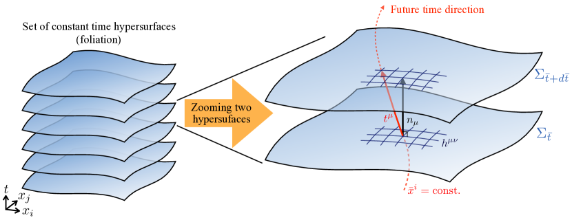
Figure 1: Illustration of the spacetime decomposition of the twistless torsional Newton-Cartan (TTNC) geometry. $\Sigma_{\bar{t}}$ denotes a hypersurface parametrized by $\bar{t}(x)=\$const., and $n_{\mu}$ is a normal vector perpendicular to the hypersurface. On each constant hypersurface, we introduce a curved spatial coordinate parametrized by $h^{\mu\nu}$ (or $h_{\mu\nu}$).

In addition, introducing the spatial coordinate systems $\bar{\bm{x}}=\bar{\bm{x}}(x)$ on $\Sigma_{\bar{t}}$, we define the time-direction vector $t^{\mu}$ by

$$t^{\mu}\equiv\partial_{\bar{t}}x^{\mu}(\bar{t},\bar{\bm{x}}).$$ (18)

While the time vector $t^{\mu}$, which determines the local time direction, does not play a central role in the Newton-Cartan geometry, it is used to define a useful gauge in Sec. 3. When we employ the new coordinate system $\{\bar{t},\bar{\bm{x}}\}$, we only have the zeroth component for the normal vector in the new coordinate systems: $n_{\bar{\mu}}=N\delta^{\bar{0}}_{\bar{\mu}}$. Therefore, the second relation in Eq. (17) reveals that $h^{\mu\nu}$ is the degenerate rank-$(d-1)$ tensor which only contains spatial components. Noting that the vector $v^{\mu}$ has a non-vanishing time component due to the first relation in Eq. (17), we can introduce the non-degenerate rank-$d$ tensor $\gamma^{\mu\nu}$ and its inverse $\gamma_{\mu\nu}$ by

$$\gamma^{\mu\nu}\equiv h^{\mu\nu}+v^{\mu}v^{\nu},\quad\gamma_{\mu\nu}\equiv h_{\mu\nu}+n_{\mu}n_{\nu},$$ (19)

where we can show they are indeed inverse by the use of all relations in Eq. (17). Leaving unfixed spatial components $v^{{\bar{i}}}$, we can explicitly write down the Newton-Cartan data in the coordinate system $\{\bar{t},\bar{\bm{x}}\}$ as

$$n_{\bar{\mu}}\equiv(N,\bm{0}),\quad v^{\bar{\mu}}\equiv\begin{pmatrix}N^{-1}\\ v^{{\bar{i}}}\end{pmatrix},\quad h_{\bar{\mu}\bar{\nu}}\equiv\begin{pmatrix}N^{2}v^{2}&-Nv_{{\bar{i}}}\\ -Nv_{{\bar{j}}}&h_{{\bar{i}}{\bar{j}}}\end{pmatrix},\quad h^{\bar{\mu}\bar{\nu}}\equiv\begin{pmatrix}0&0\\ 0&h^{{\bar{i}}{\bar{j}}}\end{pmatrix},$$ (20)

where we defined $v_{{\bar{i}}}\equiv h_{{\bar{i}}{\bar{j}}}v^{{\bar{j}}}$, and $v^{2}\equiv v^{\bar{i}}v_{{\bar{i}}}=h_{{\bar{i}}{\bar{j}}}v^{\bar{i}}v^{\bar{j}}$. Note that $h_{{\bar{i}}{\bar{j}}}$ is the inverse of $h^{{\bar{i}}{\bar{j}}}$, so that they satisfy $h_{{\bar{i}}{\bar{k}}}h^{{\bar{k}}{\bar{j}}}=\delta_{{\bar{i}}}^{{\bar{j}}}$. In this coordinate system, the non-degenerate metric $\gamma_{\bar{\mu}\bar{\nu}}$ and its inverse take forms as

$$\gamma_{\bar{\mu}\bar{\nu}}=\begin{pmatrix}N^{2}(v^{2}+1)&-Nv_{{\bar{i}}}\\ -Nv_{{\bar{j}}}&h_{{\bar{i}}{\bar{j}}}\end{pmatrix},\quad\gamma^{\bar{\mu}\bar{\nu}}=\begin{pmatrix}N^{-2}&N^{-1}v^{{\bar{i}}}\\ N^{-1}v^{{\bar{j}}}&h^{{\bar{i}}{\bar{j}}}+v^{{\bar{i}}}v^{{\bar{j}}}\end{pmatrix}.$$ (21)

Based on the above, we introduce the $d$-dimensional spacetime volume element for nonrelativistic geometry as

$$\int d^{d}x\sqrt{\gamma}=\int d^{d}xN\sqrt{h},\quad\mathrm{with}\quad\gamma\equiv\det\gamma_{\mu\nu},\quad h\equiv\det h_{{\bar{i}}{\bar{j}}}.$$ (22)

Furthermore, with the help of the normal vector $n_{\mu}$ and spatial metric $h_{\mu\nu}$, we also introduce the hypersurface vector $d\Sigma_{\bar{t}\mu}$ as

$$d\Sigma_{\bar{t}\mu}\equiv d\Sigma_{\bar{t}}n_{\mu},\quad\mathrm{with}\quad d\Sigma_{\bar{t}}\equiv d^{d-1}\bar{x}\sqrt{h},$$ (23)

where $d\Sigma_{\bar{t}}$ denotes the $(d-1)$-dimensional spatial volume element on the constant time hypersurface as is the case for relativistic geometry. The integral of the spatial volume element can be rewritten in terms of spacetime integral as follows:

$$\int d\Sigma_{\bar{t}}=\int d^{d-1}\bar{x}\sqrt{h}=\int d^{d}x\sqrt{\gamma}N^{-1}\delta(\bar{t}-\bar{t}(x)),$$ (24)

which will be used in the subsequent discussion.

In addition to the above geometric data, we introduce the covariant derivative $\nabla_{\mu}$ acting on e.g. $(1,1)$-tensor $A^{\nu}_{~{}\rho}$ as

$$\nabla_{\mu}A^{\nu}_{~{}\rho}\equiv\partial_{\mu}A^{\nu}_{~{}\rho}+\Gamma^{\nu}_{~{}\mu\sigma}A^{\sigma}_{~{}\rho}-\Gamma^{\sigma}_{~{}\mu\rho}A^{\nu}_{~{}\sigma},$$ (25)

where $\Gamma^{\mu}_{~{}\nu\rho}$ denotes a connection for the nonrelativistic curved geometry. As the metric compatibility condition $\nabla_{\mu}g_{\nu\rho}=\nabla_{\mu}g^{\nu\rho}=0$ (together with the torsion-free assumption) determines the Levi-Civita connection $\Gamma^{\mu}_{~{}\nu\rho}$, we put the compatibility condition for the Newton-Cartan data:

$$\nabla_{\mu}n_{\nu}=0,\quad\nabla_{\mu}h^{\nu\rho}=0,$$ (26)

in order to determine our nonrelativistic connection. Here note that $\nabla_{\mu}h_{\nu\rho}$ does not vanish since $h^{\mu\nu}$ is not the inverse of $h_{\mu\nu}$. Nevertheless, these compatibility conditions are not enough to determine the complete form of the connection $\Gamma^{\mu}_{~{}\nu\rho}$, and we have to put another condition to fix it. There are two competing options for the additional condition Jensen:2014aia ; Bergshoeff:2014uea : One is invariance under the $U(1)_{M}$ mass gauge transformation $a_{\mu}\to a_{\mu}+\partial_{\mu}\alpha$, and another is invariance under the so-called Milne boost transformation defined in Eq. (49) in the next subsection. These conditions are incompatible with each other and we cannot respect both of them. Following the Ref. Jensen:2014aia , we employ mass gauge invariance and use the following expressions for the connection

$$\Gamma^{\mu}_{~{}\nu\rho}\equiv v^{\mu}\partial_{\nu}n_{\rho}+\frac{1}{2}h^{\mu\sigma}\big{(}\partial_{\nu}h_{\rho\sigma}+\partial_{\rho}h_{\nu\sigma}-\partial_{\sigma}h_{\nu\rho}\big{)}+\frac{1}{2}h^{\mu\sigma}(n_{\nu}F^{a}_{\rho\sigma}+n_{\rho}F^{a}_{\nu\sigma}),$$ (27)

where we defined the field strength tensor for the $U(1)_{M}$ mass gauge field $a_{\mu}$ as

$$F^{a}_{\mu\nu}\equiv\partial_{\mu}a_{\nu}-\partial_{\nu}a_{\mu}.$$ (28)

This connection is manifestly invariant under the $U(1)_{M}$ gauge transformation but not invariant under the Milne boost transformation. The first term in Eq. (27) brings about the anti-symmetric (torsional) part of the connection:

$$\Gamma^{\mu}_{~{}\nu\rho}-\Gamma^{\mu}_{~{}\rho\nu}=v^{\mu}F^{n}_{\nu\rho},\quad\mathrm{with}\quad F^{n}_{\mu\nu}\equiv\partial_{\mu}n_{\nu}-\partial_{\nu}n_{\mu},$$ (30)

which does not vanish if $dn=F^{n}_{\mu\nu}dx^{\mu}\wedge dx^{\nu}\neq 0$.

We then show a useful formula for a later discussion:

$$\partial_{\bar{t}}\int d\Sigma_{\bar{t}\mu}f^{\mu}=\int d\Sigma_{\bar{t}}N(x)(\nabla_{\mu}-\mathcal{G}_{\mu})f^{\mu},$$ (31)

where $f^{\mu}(x)$ denotes an arbitrary smooth vector, and $\mathcal{G}_{\mu}\equiv\Gamma^{\nu}_{~{}\nu\mu}-\Gamma^{\nu}_{~{}\mu\nu}=v^{\nu}F^{n}_{\nu\mu}$ results from the torsional contribution for the covariant derivative. This formula can be derived as follows: Using Eq. (24) and the definition of the normal vector $n_{\mu}\equiv N\partial_{\mu}\bar{t}(x)$ and assuming that $f^{\mu}(x)$ vanishes at the spacetime boundary, we obtain

$$\begin{split}\int d\Sigma_{\bar{t}\mu}f^{\mu}&=\int d^{d}\bar{x}\sqrt{h}\delta(\bar{t}-\bar{t}(x))N\partial_{\mu}\bar{t}(x)f^{\mu}\\ &=-\int d^{d}\bar{x}\sqrt{\gamma}\partial_{\mu}\theta(\bar{t}-\bar{t}(x))f^{\mu}\\ &=\int d^{d}\bar{x}\sqrt{\gamma}\theta(\bar{t}-\bar{t}(x))(\nabla_{\mu}-\mathcal{G}_{\mu})f^{\mu},\end{split}$$ (32)

where we performed the integration by parts to proceed the second line and used $\partial_{\mu}\sqrt{\gamma}=\sqrt{\gamma}\,\Gamma^{\nu}_{~{}\mu\nu}=\sqrt{\gamma}(\Gamma^{\nu}_{~{}\nu\mu}-\mathcal{G}_{\mu})$. We then differentiate Eq. (32) with respect to $\bar{t}$

$$\begin{split}\partial_{\bar{t}}\int d\Sigma_{\bar{t}\mu}f^{\mu}&=\partial_{\bar{t}}\int d^{d}\bar{x}\sqrt{\gamma}\theta(\bar{t}-\bar{t}(x))(\nabla_{\mu}-\mathcal{G}_{\mu})f^{\mu}\\ &=\int d\Sigma_{\bar{t}}N(x)(\nabla_{\mu}-\mathcal{G}_{\mu})f^{\mu}.\end{split}$$ (33)

This is just Eq. (31) which we want to prove. This formula, which belongs to a family of the Stokes theorem, will be often used in the subsequent discussion.

2.2 Nonrelativistic symmetry and conservation law

We next discuss the relation between symmetries for nonrelativistic systems and its consequences like conservation laws based on gauge and coordinate reparametrization symmetry. With the help of the geometric preliminary developed in the previous section, our system is now put in the presence of the external $U(1)_{M}$ and $U(1)_{Q}$ gauge fields and background curved (TTNC) geometry. Writing all the external fields together by $j(x)=\{n_{\mu}(x),v^{\mu}(x),h_{\mu\nu}(x),h^{\mu\nu}(x),a_{\mu}(x),A_{\mu}(x)\}$, we can express our action as

$$\mathcal{S}[\varphi;j]=\int d^{d}x\sqrt{\gamma}\mathcal{L}(\varphi_{i}(x),\partial_{\mu}\varphi_{i}(x);j(x)),$$ (34)

where $\varphi_{i}$ denotes a set of dynamical matter fields under consideration, and spacetime integral covers all region where matter fields exist. For example, the explicit form of the Lagrangian for the charged and/or uncharged spinless nonlinear Schrödinger fields $\phi_{n}$ in the Newton-Cartan geometry is given by

$$\begin{split}\mathcal{L}(\phi,D_{\mu}\phi)=\sum_{n}\Bigg{[}\frac{i}{2}v^{\mu}\phi_{n}^{\dagger}\overleftrightarrow{D_{\mu}}\phi_{n}-\frac{1}{2m_{n}}h^{\mu\nu}D_{\mu}\phi_{n}^{\dagger}D_{\nu}\phi_{n}-\sum_{m}\lambda_{n,m}|\phi_{n}|^{2}|\phi_{m}|^{2}\Bigg{]},\end{split}$$ (35)

where we defined $\phi_{n}^{\dagger}\overleftrightarrow{D_{\mu}}\phi_{n}\equiv\phi_{n}^{\dagger}D_{\mu}\phi_{n}-\phi_{n}D_{\mu}\phi_{n}^{\dagger}$ with the covariant derivative $D_{\mu}$:

$$D_{\mu}\phi_{n}\equiv(\partial_{\mu}+im_{n}a_{\mu}+iq_{n}A_{\mu})\phi_{n},\quad D_{\mu}\phi_{n}^{\dagger}\equiv(\partial_{\mu}-im_{n}a_{\mu}-iq_{n}A_{\mu})\phi_{n}^{\dagger},$$ (36)

where we take a mass (electric charge) of the matter field $\phi_{n}$ as $m_{n}~{}(q_{n})$.

Let us then consider a set of infinitesimal transformation with the general coordinate transformation, $U(1)_{M}$ and $U(1)_{Q}$ gauge transformation, and the so-called Milne boost transformation driven by parameters $\chi(x)\equiv\{\xi^{\mu}(x),\alpha_{M}(x),\alpha_{Q}(x),\Lambda_{\mu}(x)\}$:

$$\begin{cases}\delta_{\chi}n_{\mu}=\xi^{\nu}\partial_{\nu}n_{\mu}+n_{\nu}\partial_{\mu}\xi^{\nu},\\ \delta_{\chi}h^{\mu\nu}=\xi^{\rho}\partial_{\rho}h^{\mu\nu}-h^{\mu\rho}\partial_{\rho}\xi^{\nu}-h^{\nu\rho}\partial_{\rho}\xi^{\mu},\\ \delta_{\chi}v^{\mu}=\xi^{\nu}\partial_{\nu}v^{\mu}-v^{\nu}\partial_{\nu}\xi^{\mu}+h^{\mu\nu}\Lambda_{\nu},\\ \delta_{\chi}h_{\mu\nu}=\xi^{\rho}\partial_{\rho}h_{\mu\nu}+h_{\mu\rho}\partial_{\nu}\xi^{\rho}+h_{\nu\rho}\partial_{\mu}\xi^{\rho}-(n_{\mu}P^{\rho}_{\nu}+n_{\nu}P^{\rho}_{\mu})\Lambda_{\rho},\\ \delta_{\chi}a_{\mu}=\xi^{\nu}\partial_{\nu}a_{\mu}+a_{\nu}\partial_{\mu}\xi^{\nu}+\partial_{\mu}\alpha_{M}-P^{\nu}_{\mu}\Lambda_{\nu},\\ \delta_{\chi}A_{\mu}=\xi^{\nu}\partial_{\nu}A_{\mu}+A_{\nu}\partial_{\mu}\xi^{\nu}+\partial_{\mu}\alpha_{Q},\\ \delta_{\chi}\varphi_{i}=\mathsterling_{\xi}\varphi_{i}-i\alpha_{M}m_{i}\varphi_{i}-i\alpha_{Q}q_{i}\varphi_{i},\end{cases}$$ (37)

where $\chi(x)=\{\xi^{\mu}(x)$, $\alpha_{M}(x),\alpha_{Q}(x),\Lambda_{\mu}(x)\}$ denotes a set of arbitrary infinitesimal vector and scalar functions which vanish at the boundary of the spacetime region, and $m_{i}~{}(q_{i})$ does the mass ($U(1)_{Q}$ charge) of the matter field $\varphi_{i}(x)$, respectively. We then consider systems whose action is invariant under these transformations : $\delta_{\chi}\mathcal{S}=0$. On the other hand, we can express $\delta_{\chi}\mathcal{S}$ in terms of variations of the action with respect to external fields. We, however, have to pay attention to the fact that all variation of the Newton-Cartan data $\{n_{\mu},h^{\mu\nu},v^{\mu},h_{\mu\nu}\}$ is not independent due to the condition (17). For example, if we take the variation of the first relation of Eqs. (17), we obtain

$$\delta(n_{\mu}v^{\mu})=v^{\mu}\delta n_{\mu}+n_{\mu}\delta v^{\mu}=0,$$ (38)

which shows that the variations of $n_{\mu}$ and $v^{\mu}$ are related with each other. Following Ref. Jensen:2014aia , we make the variation of $n_{\mu}$ to be arbitrary, and, as a consequence, the variation of $\{h^{\mu\nu},v^{\mu},h_{\mu\nu}\}$ is constrained as follows:

$$\begin{cases}\delta v^{\mu}=-v^{\mu}v^{\nu}\delta n_{\nu}+P^{\mu}_{\nu}\delta{\bar{v}}^{\nu},\\ \delta h^{\mu\nu}=-(v^{\mu}h^{\nu\rho}+v^{\nu}h^{\mu\rho})\delta n_{\rho}+P^{\mu}_{\rho}P^{\nu}_{\sigma}\delta{\bar{h}}^{\rho\sigma},\\ \delta h_{\mu\nu}=-(n_{\mu}h_{\nu\rho}+n_{\nu}h_{\mu\rho})\delta{\bar{v}}^{\rho}-h_{\mu\rho}h_{\nu\sigma}\delta{\bar{h}}^{\rho\sigma},\end{cases}$$ (39)

where $\delta{\bar{v}}^{\mu}$ and $\delta{\bar{h}}^{\mu\nu}$ are unconstrained. Taking into account this, we only have the independent variation $\{\delta n_{\mu},\delta{\bar{h}}^{\mu\nu},\delta{\bar{v}}^{\mu},\delta a_{\mu},\delta A_{\mu}\}$ as

$$\begin{cases}\delta_{\chi}n_{\mu}=\nabla_{\mu}(\xi^{\nu}n_{\nu})-F_{\mu\nu}^{n}\xi^{\nu},\\ \delta_{\chi}{\bar{h}}^{\mu\nu}=P^{\mu}_{\alpha}P^{\nu}_{\beta}\delta_{\chi}h^{\alpha\beta}=P^{\mu}_{\alpha}P^{\nu}_{\beta}(\xi^{\rho}\nabla_{\rho}h^{\alpha\beta}-h^{\alpha\rho}\nabla_{\rho}\xi^{\beta}-h^{\beta\rho}\nabla_{\rho}\xi^{\alpha}),\\ \delta_{\chi}{\bar{v}}^{\mu}=P^{\mu}_{\nu}\delta_{\chi}v^{\nu}=P^{\mu}_{\nu}(\xi^{\rho}\nabla_{\rho}v^{\nu}-v^{\rho}\nabla_{\rho}\xi^{\nu})+h^{\mu\nu}\Lambda_{\nu},\\ \delta_{\chi}a_{\mu}=\nabla_{\mu}(\xi^{\nu}a_{\nu})-F^{a}_{\mu\nu}\xi^{\nu}+\partial_{\mu}\alpha_{M}-P^{\nu}_{\mu}\Lambda_{\nu},\\ \delta_{\chi}A_{\mu}=\nabla_{\mu}(\xi^{\nu}A_{\nu})-F_{\mu\nu}\xi^{\nu}+\partial_{\mu}\alpha_{Q},\end{cases}$$ (40)

where, in addition to the field strength tensors for $a_{\mu}$ and $n_{\mu}$ defined in Eqs. (28) and (30), we further introduced the field strength tensor for $A_{\mu}$:

$$F_{\mu\nu}\equiv\partial_{\mu}A_{\nu}-\partial_{\nu}A_{\mu}.$$ (41)

Using these expressions together with the fact that variations of dynamical fields $\varphi_{i}$ does not contribute by the use of the equation of motion ($\delta\mathcal{S}/\delta\varphi_{i}=0$), we can express $\delta_{\chi}\mathcal{S}$ as

$$\begin{split}\delta_{\chi}\mathcal{S}&=\int d^{d}x\left[\frac{\delta\mathcal{S}}{\delta n_{\mu}}\delta_{\chi}n_{\mu}+\frac{\delta\mathcal{S}}{\delta{\bar{h}}^{\mu\nu}}\delta_{\chi}{\bar{h}}^{\mu\nu}+\frac{\delta\mathcal{S}}{\delta{\bar{v}}^{\mu}}\delta_{\chi}{\bar{v}}^{\mu}+\frac{\delta\mathcal{S}}{\delta a_{\mu}}\delta_{\chi}a_{\mu}+\frac{\delta\mathcal{S}}{\delta A_{\mu}}\delta_{\chi}A_{\mu}\right]\\ &=\int d^{d}x\sqrt{\gamma}\left[-\mathcal{E}^{\mu}\delta_{\chi}n_{\mu}-\frac{1}{2}T_{\mu\nu}\delta_{\chi}{\bar{h}}^{\mu\nu}-\mathcal{P}_{\mu}\delta_{\chi}{\bar{v}}^{\mu}-J_{M}^{\mu}\delta_{\chi}a_{\mu}-J_{Q}^{\mu}\delta_{\chi}A_{\mu}\right]\\ &=\int d^{d}x\sqrt{\gamma}\xi^{\nu}\Big{[}-(\nabla_{\mu}-\mathcal{G}_{\mu})\mathcal{T}^{\mu}_{~{}\nu}+J_{M}^{\mu}F^{a}_{\mu\nu}+J_{Q}^{\mu}F_{\mu\nu}-\mathcal{T}^{\mu}_{~{}\rho}(F^{n}_{\mu\nu}v^{\rho}+n_{\mu}\nabla_{\nu}v^{\rho})\\ &\hskip 70.0pt+a_{\nu}(\nabla_{\mu}-\mathcal{G}_{\mu})J_{M}^{\mu}+A_{\nu}(\nabla_{\mu}-\mathcal{G}_{\mu})J_{Q}^{\mu}\Big{]}\\ &\quad+\int d^{d}x\sqrt{\gamma}\Big{[}\alpha_{M}(\nabla_{\mu}-\mathcal{G}_{\mu})J_{M}^{\mu}+\alpha_{Q}(\nabla_{\mu}-\mathcal{G}_{\mu})J_{Q}^{\mu}-h^{\mu\nu}\Lambda_{\nu}(\mathcal{P}_{\mu}-h_{\mu\rho}J_{M}^{\rho})\Big{]}+(\mathrm{surface\ terms}),\end{split}$$ (42)

where we defined a set of conserved currents—energy current $\mathcal{E}^{\mu}$, stress tensor $T_{\mu\nu}$, momentum density $\mathcal{P}_{\mu}$, mass current $J_{M}^{\mu}$ and electric current $J_{Q}^{\mu}$—by the variation of the action with respect to external fields:

$$\mathcal{E}^{\mu}\equiv-\frac{1}{\sqrt{\gamma}}\frac{\delta\mathcal{S}}{\delta n_{\mu}},\quad T_{\mu\nu}\equiv-\frac{2}{\sqrt{\gamma}}\frac{\delta\mathcal{S}}{\delta{\bar{h}}^{\mu\nu}},\quad\mathcal{P}_{\mu}\equiv-\frac{1}{\sqrt{\gamma}}\frac{\delta\mathcal{S}}{\delta{\bar{v}}^{\mu}},\quad J_{M}^{\mu}\equiv-\frac{1}{\sqrt{\gamma}}\frac{\delta\mathcal{S}}{\delta a_{\mu}},\quad J_{Q}^{\mu}\equiv-\frac{1}{\sqrt{\gamma}}\frac{\delta\mathcal{S}}{\delta A_{\mu}}.$$ (43)

To obtain the last line in Eq. (42), we performed the integral by parts and introduced the nonrelativistic energy-momentum tensor $\mathcal{T}^{\mu}_{~{}\nu}$ defined by a combination of conserved currents,

$$\mathcal{T}^{\mu}_{~{}\nu}\equiv-\mathcal{E}^{\mu}n_{\nu}+v^{\mu}\mathcal{P}_{\nu}+T^{\mu}_{~{}\nu},$$ (44)

where we raised the index of stress tensor by $h^{\mu\nu}$: $T^{\mu}_{~{}\nu}\equiv h^{\mu\rho}T_{\rho\nu}$. Recalling that $\xi^{\nu}(x)$, $\alpha_{M}(x)$, $\alpha_{Q}(x)$ and $\Lambda_{\nu}(x)$ are arbitrary functions, invariance of the action ($\delta_{\chi}\mathcal{S}=0$) implies

$$(\nabla_{\mu}-\mathcal{G}_{\mu})\mathcal{T}^{\mu}_{~{}\nu} =J_{M}^{\mu}F^{a}_{\mu\nu}+J_{Q}^{\mu}F_{\mu\nu}-\mathcal{T}^{\mu}_{~{}\rho}(F^{n}_{\mu\nu}v^{\rho}+n_{\mu}\nabla_{\nu}v^{\rho}),$$ (45)

$$(\nabla_{\mu}-\mathcal{G}_{\mu})J_{M}^{\mu} =0,$$ (46)

$$(\nabla_{\mu}-\mathcal{G}_{\mu})J_{Q}^{\mu} =0,$$ (47)

$$\mathcal{P}_{\mu} =h_{\mu\nu}J_{M}^{\nu},$$ (48)

the operator version of which will be used as a basic building block to derive hydrodynamic equations. The first two equations provides a complete set of the nonrelativistic covariant conservation laws—Eq. (45) gives the energy-momentum conservation law, Eq. (46) the mass conservation law, and Eq. (47) the electric charge conservation law. In fact, if we see the conserved charge density associated with $\mathcal{T}^{\mu}_{~{}\nu}$, they are given by $n_{\mu}\mathcal{T}^{\mu}_{~{}\nu}=-n\cdot\mathcal{E}n_{\nu}+\mathcal{P}_{\nu}$. The first term of this represents the energy density, and the second term the momentum density. We can thus regard Eq. (45) as the nonrelativistic energy-momentum conservation laws. We, however, note that if we defined $\mathcal{T}^{\mu\nu}\equiv h^{\nu\rho}\mathcal{T}^{\mu}_{~{}\rho}$, this is not necessarily symmetric with respect to their indices: $\mathcal{T}^{\mu\nu}\neq\mathcal{T}^{\nu\mu}$. Contrary to the first three equations, the fourth equation $\eqref{eq:Milne}$ does not provide the conservation law but provides the relation between the momentum density $\mathcal{P}_{\mu}$ and the mass current $J_{M}^{\mu}$, which is well known for nonrelativistic systems. This results from the fact that the Milne boost invariance is not the dynamical symmetry of our action; in other words, as is demonstrated in Eq. (37), we do not have the transformation of the dynamical fields $\varphi_{i}$ unlike the gauge and coordinate transformations. The Milne boost invariance thus represents the redundancy how we describe the external field applied to the systems by the use of $\{v^{\mu},h_{\mu\nu},a_{\mu}\}$. Although this relation does not look so important compared to the conservation laws, it will lead to the worthwhile result that the electrical conductivity vanishes for single-component nonrelativistic systems as discussed in Sec. 4-5. We also note that our covariant action under consideration—e.g. one constructed by (35)—enjoys symmetry under the finite Milne boost transformation given by

$$\begin{cases}\delta_{\Lambda}v^{\mu}=h^{\mu\nu}\Lambda_{\nu},\\ \delta_{\Lambda}h_{\mu\nu}=-(n_{\mu}P_{\nu}^{\rho}+n_{\nu}P_{\mu}^{\rho})\Lambda_{\rho}+n_{\mu}n_{\nu}h^{\rho\sigma}\Lambda_{\rho}\Lambda_{\sigma},\\ \delta_{\Lambda}a_{\mu}=-P^{\nu}_{\mu}\Lambda_{\nu}+\dfrac{1}{2}n_{\mu}h^{\rho\sigma}\Lambda_{\rho}\Lambda_{\sigma},\end{cases}$$ (49)

where $\Lambda_{\mu}(x)$ in this equation denotes not the infinitesimal vector but the finite vector. This finite Milne boost invariance becomes important when we will consider the path-integral formula associated with local thermal equilibrium in Sec. 3.

2.3 Local Gibbs distribution

As is the case for relativistic quantum field theories Hayata:2015lga ; Hongo:2016mqm , we introduce the local Gibbs distribution for the density operator to describe the nonrelativistic system in local thermal equilibrium. The local Gibbs distribution is a generalization of the (global) Gibbs distribution employed in the grandcanonical ensemble. It provides a way to describe locally thermalized systems in terms of a set of the (intensive) local thermodynamic parameters $\lambda^{a}(x)\equiv\{\beta^{\mu}(x),\nu^{\prime}_{M}(x),\nu^{\prime}_{Q}(x)\}$ —the conjugate local thermodynamic variables, or the Lagrange multipliers to determine the average values of the conserved charge densities $\hat{c}_{a}(x)\equiv\{\hat{p}_{\nu}(x),\hat{n}_{M}^{\prime}(x),\hat{n}_{Q}^{\prime}(x)\}$ with $\hat{p}_{\nu}(x)\equiv n_{\mu}(x)\hat{\mathcal{T}}^{\mu}_{~{}\nu}(x)$, $\hat{n}_{M}^{\prime}(x)\equiv n_{\mu}(x)\hat{J}_{M}^{\mu}(x)$, and $\hat{n}_{Q}^{\prime}(x)\equiv n_{\mu}(x)\hat{J}_{Q}^{\mu}(x)$. The explicit form of the local Gibbs distribution is given by

$$\hat{\rho}_{\mathrm{LG}}[\bar{t};\lambda]\equiv\exp\left(-\hat{S}[\bar{t};\lambda]\right),\quad\mathrm{with}\quad\hat{S}[\bar{t};\lambda]\equiv\hat{K}[\bar{t};\lambda]+\Psi[\bar{t};\lambda],$$ (50)

where $\hat{K}[\bar{t};\lambda]$ is defined as

$$\begin{split}\hat{K}[\bar{t};\lambda]&\equiv-\int d\Sigma_{\bar{t}\mu}\hat{\mathcal{J}}^{\mu}_{~{}a}\lambda^{a}=-\int d\Sigma_{\bar{t}\mu}\left(\hat{\mathcal{T}}^{\mu}_{~{}\nu}(x)\beta^{\nu}(x)+\hat{J}_{M}^{\mu}(x)\nu^{\prime}_{M}(x)+\hat{J}_{Q}^{\mu}(x)\nu^{\prime}_{Q}(x)\right).\end{split}$$ (51)

Here we used the hypersurface vector $d\Sigma_{\bar{t}\mu}=d\Sigma_{\bar{t}}n_{\mu}$ introduced in the previous section, and $\hat{\mathcal{J}}^{\mu}_{~{}a}(x)\equiv\{\hat{\mathcal{T}}^{\mu}_{~{}\nu}(x),\hat{J}_{M}^{\mu}(x),\hat{J}_{Q}^{\mu}(x)\}$ denotes a set of conserved current operators. We also introduced the normalization factor $\Psi[\bar{t};\lambda,j]$ which is identified as the local thermodynamic functional, or the so-called Massieu-Planck functional:

$$\Psi[\bar{t};\lambda]=\log\mathop{\mathrm{Tr}}\exp(-\hat{K}[\bar{t};\lambda]).$$ (52)

This functional is one of the most important quantities in our formulation since it is shown to contain complete information on transport properties of systems in local thermal equilibrium; namely, as will be shown in the next section, we can extract the average value of all the conserved current operators $\langle\hat{\mathcal{J}}^{\mu}_{~{}a}(x)\rangle^{\mathrm{LG}}_{\bar{t}}$ from this single functional $\Psi[\bar{t};\lambda,j]$. Here we defined $\langle\hat{\mathcal{O}}\rangle^{\mathrm{LG}}_{\bar{t}}\equiv\mathop{\mathrm{Tr}}(\hat{\rho}_{\mathrm{LG}}[\bar{t};\lambda]\hat{\mathcal{O}})$ representing the average value of an arbitrary operator $\hat{\mathcal{O}}$ in local thermal equilibrium at time $\bar{t}$.

Before moving to the discussion on average values of conserved currents in local thermal equilibrium, we here quickly review some basic properties of thermodynamic functionals for later use. As is clear from the definition of the Massieu-Planck functional, taking variation of $\Psi[\bar{t};\lambda,j]$ with respect to $\lambda^{a}(x)$ provides the average value of the conserved charge densities over local Gibbs distribution:

$$c_{a}(x)\big{|}_{\bar{t}}\equiv\langle\hat{c}_{a}(x)\rangle^{\mathrm{LG}}_{\bar{t}}=\frac{\delta\Psi[\bar{t};\lambda]}{\delta\lambda^{a}(x)}.$$ (53)

This relation shows that the Massieu-Planck functional is properly regarded as the local thermodynamic functional. Furthermore, we introduce the entropy functional $S[\bar{t};c]$ for local thermal equilibrium as

$$\begin{split}S[\bar{t};c]&\equiv\langle\hat{S}[\bar{t};\lambda]\rangle^{\mathrm{LG}}_{\bar{t}}=-\mathop{\mathrm{Tr}}\big{(}\log\hat{\rho}_{\mathrm{LG}}[\bar{t};\lambda]\log\hat{\rho}_{\mathrm{LG}}[\bar{t};\lambda]\big{)}\\ &=-\int d\Sigma_{\bar{t}}\lambda^{a}(x)c_{a}(x)+\Psi[\bar{t};\lambda,j],\end{split}$$ (54)

which is nothing but the Legendre transformation of $\Psi[\bar{t};\lambda]$. We note that the natural variables for the entropy functional is not $\lambda^{a}(x)$ but conserved charge densities $c_{a}(x)$ as usual. This is clarified by taking a variation of the entropy functional:

$$\begin{split}\delta S&=-\int d\Sigma_{\bar{t}}\big{(}\lambda^{a}\delta c_{a}+c_{a}\delta\lambda^{a}\big{)}+\delta\Psi[\bar{t};\lambda,j]\\ &=-\int d\Sigma_{\bar{t}}\big{(}\lambda^{a}(x)\delta c_{a}(x)+c_{a}(x)\delta\lambda^{a}(x)\big{)}+\int d\Sigma_{\bar{t}}\delta\lambda^{a}(x)\frac{\delta\Psi[\bar{t};\lambda]}{\delta\lambda^{a}(x)}\\ &=-\int d\Sigma_{\bar{t}}\lambda^{a}(x)\delta c_{a}(x)\end{split}$$ (56)

where we used Eq. (53) to proceed the last line. We therefore obtain the following formula for local thermodynamics parameters $\lambda^{a}(x)$:

$$\lambda^{a}(x)\big{|}_{\bar{t}}=-\frac{\delta S[\bar{t};c]}{\delta c_{a}(x)}.$$ (57)

It is worthwhile to emphasize that we have the one-to-one correspondence between the local thermodynamic parameters $\lambda^{a}(x)$ and the averaged conserved charge densities $c_{a}(x)$ owing to the convexity of the Massieu-Planck functional $\Psi[\bar{t};\lambda,j]$.

3 Path-integral formula for local thermal equilibrium

In this section, we develop the imaginary-time path-integral formalism for spinless Schrödinger fields in local thermal equilibrium, which enables us to evaluate nondissipative part of constitutive relations (See Ref. Hongo:2016mqm in the relativistic case). In Sec. 3.1, we first show that the Massieu-Planck functional is regarded as a generating functional for the average value of conserved current operators over the local Gibbs distribution $\langle\hat{\mathcal{J}}^{\mu}_{~{}a}(x)\rangle^{\mathrm{LG}}_{\bar{t}}$. We provide the exact variational formula based on invariance of the functional operator $\hat{K}[\bar{t};\lambda]$. We also introduce a useful gauge choice, a hydrostatic gauge, which simplify our calculation. In Sec. 3.2, explicitly dealing with spinless Bosonic and Fermionic Schrödinger fields, we obtain the path-integral formula for the Massieu-Planck functional, and show that it is written in terms of quantum field theories in the thermally emergent Newton-Cartan geometry. In Sec. 3.3, we summarize the symmetry properties of the Massieu-Planck functional.

3.1 Variational formula for nondissipative constitutive relation

Here we provide the variational formula for the Massieu-Planck functional and show that it is regarded as a generating functional for $\langle\hat{\mathcal{J}}^{\mu}_{~{}a}(x)\rangle^{\mathrm{LG}}_{\bar{t}}$. After deriving the variational formula without a gauge fixing in Sec. 3.1.1, we introduce the useful gauge which we call hydrostatic gauge in Sec. 3.1.2.

3.1.1 Derivation of variational formula in general setup

We here show the derivation of the variational formula in a general setup without gauge fixing. First of all, we rewrite $\hat{K}[\bar{t};\lambda]$ as

$$\begin{split}\hat{K}[\bar{t},\lambda,j]=\int d^{d}x\delta(\bar{t}-\bar{t}(x))\hat{\kappa}(\lambda^{a},j),\quad\mathrm{with}\quad\hat{\kappa}(\lambda^{a},j)\equiv\sqrt{\gamma}N^{-1}n_{\mu}\hat{\mathcal{J}}^{\mu}_{~{}a}\lambda^{a},\end{split}$$ (58)

from which we can see that this functional operator is manifestly invariant under the coordinate reparametrization. In order to emphasize arguments of functional operator $\hat{K}[\bar{t};\lambda]$, we explicitly write down them. We also note that this functional operator is $U(1)_{M}$ and $U(1)_{Q}$ gauge invariant. Let us then consider the combination of the infinitesimal coordinate reparametrization and $U(1)_{M,Q}$ gauge transformation to the specific direction whose parameters are given by $\xi^{\mu}(x)=\epsilon\beta^{\mu}(x)$, $\alpha_{M}(x)=-\epsilon(\nu^{\prime}_{M}+\beta\cdot a)$, and $\alpha_{Q}(x)=-\epsilon(\nu^{\prime}_{Q}+\beta\cdot A)$. Invariance of $\hat{K}[\bar{t},\lambda,j]$ under this transformation leads to the following operator identity

$$\delta_{\lambda}\hat{K}[\bar{t},\lambda,j]\equiv\hat{K}[\bar{t}+\epsilon\mathsterling_{\beta}\bar{t},\lambda^{a}+\mathsterling_{\beta}\lambda^{a},j+\epsilon\delta_{\lambda}j]-\hat{K}[\bar{t},\lambda^{a},j]=0,$$ (59)

where $\mathsterling_{\beta}$ denotes the Lie derivative along $\beta^{\mu}$. We write the variation of external fields as $\delta_{\lambda}j$ to reveal that our variation of the $U(1)_{M,Q}$ gauge field is not a simple Lie derivative but given by

$$\delta_{\lambda}a_{\mu} \equiv\mathsterling_{\beta}a_{\mu}-\nabla_{\mu}(\nu^{\prime}_{M}+\beta\cdot a)=-\beta^{\nu}F^{a}_{\mu\nu}-\nabla_{\mu}\nu^{\prime}_{M},$$ (60)

$$\delta_{\lambda}A_{\mu} \equiv\mathsterling_{\beta}A_{\mu}-\nabla_{\mu}(\nu^{\prime}_{Q}+\beta\cdot A)=-\beta^{\nu}F_{\mu\nu}-\nabla_{\mu}\nu^{\prime}_{Q},$$ (61)

while the variations of the other external fields, or the Newton-Cartan data is simply given by their Lie derivatives: e.g. $\delta_{\lambda}n_{\mu}=\mathsterling_{\beta}n_{\mu}$. We note that the lie derivatives of $\nu_{M,Q}$ are expressed as $\mathsterling_{\beta}\nu^{\prime}_{M}=-\beta^{\mu}\delta_{\lambda}a_{\mu}$ and $\mathsterling_{\beta}\nu^{\prime}_{Q}=-\beta^{\mu}\delta_{\lambda}A_{\mu}$ due to Eqs. (60)-(61). Based on these, we can express $\delta_{\lambda}\hat{K}[\bar{t},\lambda,j]$ in terms of the variations as

$$\begin{split}\delta_{\lambda}\hat{K}&=\int d^{d}x\epsilon\left[\frac{\delta\hat{K}}{\delta\bar{t}(x)}\mathsterling_{\beta}\bar{t}(x)+\frac{\delta\hat{K}}{\delta\lambda^{a}(x)}\mathsterling_{\beta}\lambda^{a}(x)+\frac{\delta\hat{K}}{\delta j_{a}(x)}\delta_{\lambda}j_{a}(x)\right]\\ &=\int d^{d}x\epsilon\Bigg{[}\sqrt{\gamma}\delta(\bar{t}-\bar{t}(x))\left(\hat{\mathcal{E}}^{\mu}\mathsterling_{\beta}n_{\mu}+\hat{\mathcal{P}}_{\mu}\mathsterling_{\beta}{\bar{v}}^{\mu}+\frac{1}{2}\hat{T}_{\mu\nu}\mathsterling_{\beta}{\bar{h}}^{\mu\nu}+\hat{J}_{M}^{\mu}\delta_{\lambda}a_{\mu}+\hat{J}_{Q}^{\mu}\delta_{\lambda}A_{\mu}\right)\beta^{\mu}\partial_{\mu}\bar{t}\\ &\hskip 24.0pt+\frac{\delta\hat{K}}{\delta n_{\mu}}\mathsterling_{\beta}n_{\mu}+\frac{\delta\hat{K}}{\delta{\bar{v}}^{\mu}}\mathsterling_{\beta}{\bar{v}}^{\mu}+\frac{\delta\hat{K}}{\delta{\bar{h}}^{\mu\nu}}\mathsterling_{\beta}{\bar{h}}^{\mu\nu}+\left(\frac{\delta\hat{K}}{\delta a_{\mu}}-\frac{\delta\hat{K}}{\delta\nu^{\prime}_{M}}\beta^{\mu}\right)\delta_{\lambda}a_{\mu}+\left(\frac{\delta\hat{K}}{\delta A_{\mu}}-\frac{\delta\hat{K}}{\delta\nu^{\prime}_{Q}}\beta^{\mu}\right)\delta_{\lambda}A_{\mu}\Bigg{]}\\ &=\int d^{d}x\epsilon\Bigg{[}\left(\beta\sqrt{h}\,\hat{\mathcal{E}}^{\mu}\big{|}_{\bar{t}}+\frac{\delta\hat{K}}{\delta n_{\mu}}\right)\mathsterling_{\beta}n_{\mu}+\left(\beta\sqrt{h}\hat{\mathcal{P}}_{\mu}\big{|}_{\bar{t}}+\frac{\delta\hat{K}}{\delta{\bar{v}}^{\mu}}\right)\mathsterling_{\beta}{\bar{v}}^{\mu}+\left(\frac{\beta\sqrt{h}}{2}\hat{T}_{\mu\nu}\big{|}_{\bar{t}}+\frac{\delta\hat{K}}{\delta{\bar{h}}^{\mu\nu}}\right)\mathsterling_{\beta}{\bar{h}}^{\mu\nu}\\ &\hskip 42.0pt+\left(\beta\sqrt{h}\hat{J}_{M}^{\mu}\big{|}_{\bar{t}}-\frac{\delta\hat{K}}{\delta\nu^{\prime}_{M}}\beta^{\mu}+\frac{\delta\hat{K}}{\delta a_{\mu}}\right)\delta_{\lambda}a_{\mu}+\left(\beta\sqrt{h}\hat{J}_{Q}^{\mu}\big{|}_{\bar{t}}-\frac{\delta\hat{K}}{\delta\nu^{\prime}_{Q}}\beta^{\mu}+\frac{\delta\hat{K}}{\delta A_{\mu}}\right)\delta_{\lambda}A_{\mu}\Bigg{]},\end{split}$$ (62)

where we defined $\beta(x)\equiv n_{\mu}(x)\beta^{\mu}(x)=N(x)\beta^{{\bar{0}}}(x)$ and used the following expression for the first term in the first line:

$$\begin{split}\frac{\delta\hat{K}}{\delta\bar{t}(x)}&=\frac{\delta}{\delta\bar{t}(x)}\int d^{d}x\sqrt{\gamma}\theta(\bar{t}-\bar{t}(x))(\nabla_{\mu}-\mathcal{G}_{\mu})(\hat{\mathcal{J}}^{\mu}_{~{}a}\lambda^{a})\\ &=-\int d^{d}x\sqrt{\gamma}\delta(\bar{t}-\bar{t}(x))(\nabla_{\mu}-\mathcal{G}_{\mu})(\hat{\mathcal{J}}^{\mu}_{~{}a}\lambda^{a})\\ &=\int d^{d}x\sqrt{\gamma}\delta(\bar{t}-\bar{t}(x))\left(\hat{\mathcal{E}}^{\mu}\mathsterling_{\beta}n_{\mu}+\hat{\mathcal{P}}_{\mu}\mathsterling_{\beta}v^{\mu}+\frac{1}{2}\hat{T}_{\mu\nu}\mathsterling_{\beta}h^{\mu\nu}+\hat{J}_{M}^{\mu}\delta_{\lambda}a_{\mu}+\hat{J}_{Q}^{\mu}\delta_{\lambda}A_{\mu}\right).\end{split}$$ (63)

Here we used Eq. (32) to rewrite $\hat{K}[\bar{t},\lambda,j]$ by the use of the step function $\theta(\bar{t}-\bar{t}(x))$, and substitute the following results for the covariant divergence of $\hat{\mathcal{J}}^{\mu}_{~{}a}\lambda^{a}$ with the help of the conservation laws (45)-(47):

$$\begin{split}(\nabla_{\mu}-\mathcal{G}_{\mu})\big{(}\hat{\mathcal{J}}^{\mu}_{~{}a}\lambda^{a}\big{)}&=\hat{\mathcal{T}}^{\mu}_{~{}\nu}\Big{(}\nabla_{\mu}\beta^{\nu}-\beta^{\rho}(F^{n}_{\mu\rho}v^{\nu}+n_{\mu}\nabla_{\rho}v^{\nu})\Big{)}+\hat{J}_{M}^{\mu}(\beta^{\nu}F^{a}_{\mu\nu}+\nabla_{\mu}\nu^{\prime}_{M})+\hat{J}_{Q}^{\mu}(\beta^{\nu}F_{\mu\nu}+\nabla_{\mu}\nu^{\prime}_{Q})\\ &=(-\hat{\mathcal{E}}^{\mu}n_{\nu}+v^{\mu}\hat{\mathcal{P}}_{\nu}+\hat{T}^{\mu}_{~{}\nu})\nabla_{\mu}\beta^{\nu}+\hat{\mathcal{E}}^{\mu}F^{n}_{\mu\nu}\beta^{\nu}-\hat{\mathcal{P}}_{\mu}\beta^{\nu}\nabla_{\nu}v^{\mu}-\hat{J}_{M}^{\mu}\delta_{\lambda}a_{\mu}-\hat{J}_{Q}^{\mu}\delta_{\lambda}A_{\mu}\\ &=-\hat{\mathcal{E}}^{\mu}\mathsterling_{\beta}n_{\mu}-\hat{\mathcal{P}}_{\mu}\mathsterling_{\beta}{\bar{v}}^{\mu}-\frac{1}{2}\hat{T}_{\mu\nu}\mathsterling_{\beta}{\bar{h}}^{\mu\nu}-\hat{J}_{M}^{\mu}\delta_{\lambda}a_{\mu}-\hat{J}_{Q}^{\mu}\delta_{\lambda}A_{\mu}.\end{split}$$ (64)

We then take average of Eq. (62) over the local Gibbs distribution at that time $\bar{t}$, which results in

$$\begin{split}\langle\delta_{\lambda}\hat{K}\rangle^{\mathrm{LG}}_{\bar{t}}&=\int d^{d}x\epsilon\Bigg{[}\left(\beta\sqrt{h}\langle\hat{\mathcal{E}}^{\mu}\rangle^{\mathrm{LG}}_{\bar{t}}-\frac{\delta\Psi}{\delta n_{\mu}}\right)\mathsterling_{\beta}n_{\mu}\\ &\hskip 42.0pt+\left(\beta\sqrt{h}\langle\hat{\mathcal{P}}_{\mu}\rangle^{\mathrm{LG}}_{\bar{t}}-\frac{\delta\Psi}{\delta{\bar{v}}^{\mu}}\right)\mathsterling_{\beta}{\bar{v}}_{\mu}+\left(\frac{\beta\sqrt{h}}{2}\langle\hat{T}_{\mu\nu}\rangle^{\mathrm{LG}}_{\bar{t}}-\frac{\delta\Psi}{\delta{\bar{h}}^{\mu\nu}}\right)\mathsterling_{\beta}{\bar{h}}^{\mu\nu}\\ &\hskip 42.0pt+\left(\beta\sqrt{h}\langle\hat{J}_{M}^{\mu}\rangle^{\mathrm{LG}}_{\bar{t}}+\frac{\delta\Psi}{\delta\nu^{\prime}_{M}}\beta^{\mu}-\frac{\delta\Psi}{\delta a_{\mu}}\right)\delta_{\lambda}a_{\mu}+\left(\beta\sqrt{h}\langle\hat{J}_{Q}^{\mu}\rangle^{\mathrm{LG}}_{\bar{t}}+\frac{\delta\Psi}{\delta\nu^{\prime}_{Q}}\beta^{\mu}-\frac{\delta\Psi}{\delta A_{\mu}}\right)\delta_{\lambda}A_{\mu}\Bigg{]},\end{split}$$ (65)

where we replaced the average value of the variation of $\hat{K}[\bar{t},\lambda,j]$ with respect to external fields as the variation of the Massieu-Planck functional. Therefore, using the identity $\langle\delta_{\lambda}\hat{K}\rangle^{\mathrm{LG}}_{\bar{t}}=0$, we have eventually obtained a set of the variational formulae for the Massieu-Planck functional:

$$\begin{cases}\langle\hat{\mathcal{E}}^{\mu}(x)\rangle^{\mathrm{LG}}_{\bar{t}}=\dfrac{1}{\beta\sqrt{h}}\dfrac{\delta\Psi[\bar{t};\lambda,j]}{\delta n_{\mu}(x)},\vspace{5pt}\\ \langle\hat{\mathcal{P}}_{\mu}(x)\rangle^{\mathrm{LG}}_{\bar{t}}=\dfrac{1}{\beta\sqrt{h}}\dfrac{\delta\Psi[\bar{t};\lambda,j]}{\delta{\bar{v}}^{\mu}(x)},\vspace{5pt}\\ \langle\hat{T}_{\mu\nu}(x)\rangle^{\mathrm{LG}}_{\bar{t}}=\dfrac{2}{\beta\sqrt{h}}\dfrac{\delta\Psi[\bar{t};\lambda,j]}{\delta{\bar{h}}^{\mu\nu}(x)},\\ \end{cases}\quad\begin{cases}\langle\hat{J}_{M}^{\mu}(x)\rangle^{\mathrm{LG}}_{\bar{t}}=-\dfrac{1}{\beta\sqrt{h}}\left(\dfrac{\delta\Psi[\bar{t};\lambda,j]}{\delta\nu^{\prime}_{M}(x)}\beta^{\mu}-\dfrac{\delta\Psi[\bar{t};\lambda,j]}{\delta a_{\mu}(x)}\right),\vspace{5pt}\\ \langle\hat{J}_{Q}^{\mu}(x)\rangle^{\mathrm{LG}}_{\bar{t}}=-\dfrac{1}{\beta\sqrt{h}}\left(\dfrac{\delta\Psi[\bar{t};\lambda,j]}{\delta\nu^{\prime}_{Q}(x)}\beta^{\mu}-\dfrac{\delta\Psi[\bar{t};\lambda,j]}{\delta A_{\mu}(x)}\right),\end{cases}$$ (66)

Combining the first three equations we can construct the variational formula for nonrelativistic energy-momentum tensor as

$$\langle\hat{\mathcal{T}}^{\mu}_{~{}\nu}(x)\rangle^{\mathrm{LG}}_{\bar{t}} =\frac{1}{\beta\sqrt{h}}\left(-\frac{\delta\Psi[\bar{t};\lambda,j]}{\delta n_{\mu}(x)}n_{\nu}(x)+v^{\mu}(x)\frac{\delta\Psi[\bar{t};\lambda,j]}{\delta{\bar{v}}^{\nu}(x)}+2h^{\mu\rho}(x)\frac{\delta\Psi[\bar{t};\lambda,j]}{\delta{\bar{h}}^{\rho\nu}(x)}\right).$$ (67)

These variational formulae relate the expectation values of all the conserved charge currents in local thermal equilibrium to the single functional $\Psi[\bar{t};\lambda,j]$. Therefore, once we evaluate the Massieu-Planck functional $\Psi[\bar{t};\lambda,j]$, we can immediately calculate the average values of the conserved current operators over the local Gibbs distribution by the use of these formulae. We thus only need to evaluate the Massieu-Planck functional $\Psi[\bar{t};\lambda,j]$ to obtain $\langle\hat{\mathcal{J}}^{\mu}_{~{}a}(x)\rangle^{\mathrm{LG}}_{\bar{t}}$. Note that these variational formulae are exact in the sense that we do not perform the derivative expansion at this stage. Of course, in order to derive the usual hydrodynamic equations in Sec. 5, we will perform the derivative expansion of $\Psi[\bar{t};\lambda,j]$. Nevertheless, this formula can be applied in more general situations where some components of derivative expansion breaks down.

3.1.2 Variational formula in the hydrostatic gauge

In the previous subsection, we derived the variational formulae (66) in the general setup without choosing any special coordinate system or special gauge. Although variational formulae (66) tell us complete information on nondissipative transports taking place in local thermal equilibrium, it is more useful to reexpress them in a special gauge which we call the hydrostatic gauge. Furthermore, it is also notable that we can considerably simplify the derivation of variation formulae in that gauge. Thus, we here rederive and reexpress the variational formulae for the Massieu-Planck functional in the hydrostatic gauge.

The key identity in our discussion is the time derivative of the Massieu-Planck functional:

$$\begin{split}\partial_{\bar{t}}\Psi[\bar{t};\lambda,j]&=-\langle\partial_{\bar{t}}\hat{K}[\bar{t};\lambda,j]\rangle^{\mathrm{LG}}_{\bar{t}}=\Big{\langle}\partial_{\bar{t}}\int d\Sigma_{\bar{t}\mu}\hat{\mathcal{J}}^{\mu}_{~{}a}\lambda^{a}\Big{\rangle}^{\mathrm{LG}}_{\bar{t}}\\ &=\Big{\langle}\int d\Sigma_{\bar{t}}N(\nabla_{\mu}-\mathcal{G}_{\mu})\big{(}\hat{\mathcal{J}}^{\mu}_{~{}a}\lambda^{a}\big{)}\Big{\rangle}^{\mathrm{LG}}_{\bar{t}}\\ &=-\Big{\langle}\int d\Sigma_{\bar{t}}N\Big{(}\hat{\mathcal{E}}^{\mu}\mathsterling_{\beta}n_{\mu}+\hat{\mathcal{P}}_{\mu}\mathsterling_{\beta}{\bar{v}}^{\mu}+\frac{1}{2}\hat{T}_{\mu\nu}\mathsterling_{\beta}{\bar{h}}^{\mu\nu}+\hat{J}_{M}^{\mu}\delta_{\lambda}a_{\mu}+\hat{J}_{Q}^{\mu}\delta_{\lambda}A_{\mu}\Big{)}\Big{\rangle}^{\mathrm{LG}}_{\bar{t}},\end{split}$$ (68)

where we used Stokes theorem (31) and Eq. (64) to proceed the second and third line, respectively. This is a general identity without gauge fixing. Then, let us introduce the hydrostatic gauge by matching the time-direction vector $t^{\mu}(x)$ in Eq. (18), and zeroth component of gauge fields $a_{\bar{0}}(x)=t^{\mu}(x)a_{\mu}(x)$ and $A_{\bar{0}}=t^{\mu}(x)A_{\mu}(x)$ with local thermodynamic parameters $\lambda^{a}(x)$:

$$t^{\mu}(x)=\beta^{\mu}(x)/\beta_{0},\quad a_{\bar{0}}(x)=-\nu^{\prime}_{M}(x)/\beta_{0},\quad A_{\bar{0}}(x)=-\nu^{\prime}_{Q}(x)/\beta_{0},$$ (69)

where $\beta_{0}$ denotes an arbitrary constant, or reference inverse temperature. This equation is a hydrostatic gauge fixing condition. The second and third conditions in Eq. (69) are common; it means that we can regard the chemical potential as the zeroth component of corresponding gauge fields in the hydrostatic gauge. The first equation enables us to see our inhomogeneous fluid configurations in an extremely simplified way. Indeed, as is shown in Fig. 2, our fluid vector $\beta^{\mu}(x)$ becomes a homogeneous constant vector directed to the time direction in the hydrostatic $(\bar{t},\bar{\bm{x}})$-coordinate. Thus, in this coordinate system, the fluid looks entirely at rest, which is the origin of the name hydrostatic gauge. Nevertheless, it is important to emphasize that our system is, in general, not stationary at all contrary to its hydrostatic appearance. This results from the fact that our fluid vector $\beta^{\mu}$, or the time-direction vector $t^{\mu}$ in the hydrostatic gauge, is not a killing vector: $\mathsterling_{t}g_{\mu\nu}\neq 0$. Therefore, to choose the hydrostatic gauge in the whole spacetime, we need to track the time-dependent fluid vector $\beta^{\mu}$ to match it with the time-direction vector at every moment.

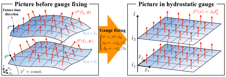
Figure 2: Schematic picture of the hydrostatic gauge fixing. While we have an arbitrary inhomogeneous fluid vector configuration $\beta^{\mu}(x)$ before the hydrostatic gauge fixing (left figure), we have homogeneously ordered fluid vector $\beta^{{\bar{\mu}}}(x)\big{|}_{\mathrm{hs}}=\beta_{0}\delta^{{\bar{\mu}}}_{\bar{0}}$ in the hydrostatic gauge (right figure).

Then, let us derive the variational formula in the hydrostatic gauge. Thanks to the hydrostatic gauge condition (69), we can replace $\delta_{\lambda}a_{\mu}$ and $\delta_{\lambda}A_{\mu}$ in the hydrostatic gauge by the simple lie derivatives:

$$\begin{split}\delta_{\lambda}a_{\mu}\big{|}_{\mathrm{hs}}&=\mathsterling_{\beta}a_{\mu}-\nabla_{\mu}(\nu_{M}^{\prime}+\beta\cdot a)\big{|}_{\nu_{M}^{\prime}=-\beta\cdot a}=\mathsterling_{\beta}a_{\mu},\\ \delta_{\lambda}A_{\mu}\big{|}_{\mathrm{hs}}&=\mathsterling_{\beta}A_{\mu}-\nabla_{\mu}(\nu_{Q}^{\prime}+\beta\cdot a)\big{|}_{\nu_{Q}^{\prime}=-\beta\cdot A}=\mathsterling_{\beta}A_{\mu}.\end{split}$$ (70)

Using these relations together with $\mathsterling_{t}=(\beta_{0})^{-1}\mathsterling_{\beta}\beta^{\mu}$ which also results from the gauge fixing condition (69), we obtain the following expression for $\partial_{\bar{t}}\Psi[\bar{t};\lambda,j]$:

$$\begin{split}\partial_{\bar{t}}\Psi[\bar{t};j]\big{|}_{\mathrm{hs}}&=-\int d^{d-1}\bar{x}\sqrt{\gamma}\beta_{0}\Big{(}\langle\hat{\mathcal{E}}^{\mu}\rangle^{\mathrm{LG}}_{\bar{t}}\mathsterling_{t}n_{\mu}+\langle\hat{\mathcal{P}}_{\mu}\rangle^{\mathrm{LG}}_{\bar{t}}\mathsterling_{t}{\bar{v}}^{\mu}+\frac{1}{2}\langle\hat{T}_{\mu\nu}\rangle^{\mathrm{LG}}_{\bar{t}}\mathsterling_{t}{\bar{h}}^{\mu\nu}+\langle\hat{J}_{M}^{\mu}\rangle^{\mathrm{LG}}_{\bar{t}}\mathsterling_{t}a_{\mu}+\langle\hat{J}_{Q}^{\mu}\rangle^{\mathrm{LG}}_{\bar{t}}\mathsterling_{t}A_{\mu}\Big{)}.\end{split}$$ (71)

On the other hand, the left-hand-side of this equation is nothing but the lie derivative of the Massieu-Planck functional $\Psi[\bar{t};j]\big{|}_{\mathrm{hs}}$ along the time-direction vector $t^{\mu}$, and thus, we can simply express it in terms of variations as

$$\begin{split}\partial_{\bar{t}}\Psi[\bar{t};j]\big{|}_{\mathrm{hs}}&=\int d^{d-1}\bar{x}\left(\frac{\delta\Psi}{\delta n_{\mu}}\mathsterling_{t}n_{\mu}+\frac{\delta\Psi}{\delta{\bar{v}}^{\mu}}\mathsterling_{t}{\bar{v}}^{\mu}+\frac{\delta\Psi}{\delta{\bar{h}}^{\mu\nu}}\mathsterling_{t}{\bar{h}}^{\mu\nu}+\frac{\delta\Psi}{\delta a_{\mu}}\mathsterling_{t}a_{\mu}+\frac{\delta\Psi}{\delta A_{\mu}}\mathsterling_{t}A_{\mu}\right).\end{split}$$ (72)

Therefore, matching these equation immediately provides the following simple variational formulae in the hydrostatic gauge:

$$\begin{cases}\langle\hat{\mathcal{E}}^{\mu}(x)\rangle^{\mathrm{LG}}_{\bar{t}}=-\dfrac{1}{\beta_{0}\sqrt{\gamma}}\dfrac{\delta\Psi[\bar{t};j]}{\delta n_{\mu}(x)}\Bigg{|}_{\mathrm{hs}},\vspace{5pt}\\ \langle\hat{\mathcal{P}}_{\mu}(x)\rangle^{\mathrm{LG}}_{\bar{t}}=-\dfrac{1}{\beta_{0}\sqrt{\gamma}}\dfrac{\delta\Psi[\bar{t};j]}{\delta{\bar{v}}^{\mu}(x)}\Bigg{|}_{\mathrm{hs}},\vspace{5pt}\\ \langle\hat{T}_{\mu\nu}(x)\rangle^{\mathrm{LG}}_{\bar{t}}=-\dfrac{2}{\beta_{0}\sqrt{\gamma}}\dfrac{\delta\Psi[\bar{t};j]}{\delta{\bar{h}}^{\mu\nu}(x)}\Bigg{|}_{\mathrm{hs}},\end{cases}\quad\begin{cases}\langle\hat{J}_{M}^{\mu}(x)\rangle^{\mathrm{LG}}_{\bar{t}}=-\dfrac{1}{\beta_{0}\sqrt{\gamma}}\dfrac{\delta\Psi[\bar{t};j]}{\delta a_{\mu}(x)}\Bigg{|}_{\mathrm{hs}},\vspace{5pt}\\ \langle\hat{J}_{Q}^{\mu}(x)\rangle^{\mathrm{LG}}_{\bar{t}}=-\dfrac{1}{\beta_{0}\sqrt{\gamma}}\dfrac{\delta\Psi[\bar{t};j]}{\delta A_{\mu}(x)}\Bigg{|}_{\mathrm{hs}}.\end{cases}$$ (73)

From these variational formulae, we see that the Massieu-Planck functional in the hydrostatic gauge $\Psi[\bar{t};j]\big{|}_{\mathrm{hs}}$ simply serves as a generating functional (or a kind of the action) for the conserved current operator averaged over the local Gibbs distribution (See Eq. (43) for the definition of the microscopic current operators). Again, combining the first three equation enables us to evaluate the nonrelativistic energy-momentum tensor in local thermal equilibrium as follows:

$$\langle\hat{\mathcal{T}}^{\mu}_{~{}\nu}(x)\rangle^{\mathrm{LG}}_{\bar{t}}=-\frac{1}{\beta_{0}\sqrt{\gamma}}\left(-\frac{\delta\Psi[\bar{t};j]}{\delta n_{\mu}(x)}\Bigg{|}_{\mathrm{hs}}n_{\nu}(x)+v^{\mu}(x)\frac{\delta\Psi[\bar{t};j]}{\delta{\bar{v}}^{\nu}(x)}\Bigg{|}_{\mathrm{hs}}+2h^{\mu\rho}(x)\frac{\delta\Psi[\bar{t};j]}{\delta{\bar{h}}^{\rho\nu}(x)}\Bigg{|}_{\mathrm{hs}}\right).$$ (74)

When we will perform the derivative expansion and derive the hydrodynamic equation in Sec. 5, we will use these variational formulae instead of the general ones (66).

3.2 Path-integral formula and thermally emergent Newton-Cartan geometry

As demonstrated in the previous section, we can extract information on all the conserved currents in local thermal equilibrium from the single functional $\Psi[\bar{t};\lambda,j]$. Then, the problem is reduced to evaluating this functional based on underlying quantum theories. In this section, dealing with the spinless Bosonic or Fermionic Schrödinger field as a concrete example, we write down the path-integral formula for $\Psi[\bar{t};\lambda,j]$, which brings about the emergence of thermally induced curved spacetime. Since we are considering nonrelativistic systems, emergent thermal spacetime is not the (pseudo) Riemannian geometry but the Newton-Cartan geometry.

The Lagrangian for the single-component interacting spinless Bosonic or Schrödinger field $\phi$ in the nonrelativistic curved spacetime reads

$$\begin{split}\mathcal{S}[\phi;j]&=\int d^{d}x\sqrt{\gamma}\left[\frac{i}{2}v^{\mu}\phi^{\dagger}\overleftrightarrow{D_{\mu}}\phi-\frac{1}{2m}h^{\mu\nu}D_{\mu}\phi^{\dagger}D_{\nu}\phi\right]+\mathcal{S}_{\mathrm{int}}[\phi;j]\end{split}$$ (75)

where we defined $\phi^{\dagger}\overleftrightarrow{D_{\mu}}\phi\equiv\phi^{\dagger}D_{\mu}\phi-\phi D_{\mu}\phi^{\dagger}$ with the covariant derivative $D_{\mu}$ acting on $\phi$ and $\phi^{\dagger}$ as

$$D_{\mu}\phi\equiv(\partial_{\mu}+ima_{\mu}+ieA_{\mu})\phi,\quad D_{\mu}\phi^{\dagger}\equiv(\partial_{\mu}-ima_{\mu}-ieA_{\mu})\phi^{\dagger}.$$ (76)

Here $\mathcal{S}_{\mathrm{int}}[\phi;j]$ contains interaction terms of our system: For example, while $\mathcal{S}_{\mathrm{int}}=-\dfrac{1}{2}\displaystyle{\int}d^{d}x\sqrt{\gamma}\lambda|\phi|^{4}$ describes the nonlinear Schrödinger field realized in cold atom systems, we can also describe systems with long range interaction in the covariant manner—e.g. systems interacting through the Lennard-Jones potential—by the use of auxiliary massless field living in extra dimensions (See e.g. Hoyos:2011ez ; Fujii:2016mbc for such a treatment). The essential point here is that we assume that $\mathcal{S}_{\mathrm{int}}[\phi;j]$ respects diffeomorphism, gauge, and Milne boost invariance as is the case of for the above two examples. We then have the corresponding covariant conservation laws, or the operator identities (45)-(48) with a set of conserved current defined in Eq. $\eqref{eq:Jset}$. In the following discussion, we consider the nonlinear Schrödinger fields as a concrete example:

$$\mathcal{S}[\phi;j]=\int d^{d}x\sqrt{\gamma}\mathcal{L},\quad\mathrm{with}\quad\mathcal{L}\equiv\frac{i}{2}v^{\mu}\phi^{\dagger}\overleftrightarrow{D_{\mu}}\phi-\frac{1}{2m}h^{\mu\nu}D_{\mu}\phi^{\dagger}D_{\nu}\phi-\frac{1}{2}\lambda|\phi|^{4}.$$ (77)

Then, taking variations of this action brings about a following set of conserved current operators:

$$\hat{\mathcal{E}}^{\mu} \equiv-\frac{1}{\sqrt{\gamma}}\frac{\delta\mathcal{S}}{\delta n_{\mu}}=v^{\mu}\left[\frac{1}{2m}h^{\mu\nu}D_{\mu}\hat{\phi}^{\dagger}D_{\nu}\hat{\phi}+\frac{1}{2}\lambda|\hat{\phi}|^{4}\right]-\frac{1}{2m}\big{(}h^{\mu\sigma}v^{\rho}+h^{\mu\sigma}v^{\sigma}\big{)}D_{\rho}\hat{\phi}^{\dagger}D_{\sigma}\hat{\phi},$$ (78)

$$\hat{\mathcal{P}}_{\mu} \equiv-\frac{1}{\sqrt{\gamma}}\frac{\delta\mathcal{S}}{\delta\bar{v}^{\mu}}=-\frac{i}{2}\hat{\phi}^{\dagger}\overleftrightarrow{D_{\perp}}_{\mu}\hat{\phi},$$ (79)

$$\hat{T}_{\mu\nu} \equiv-\frac{2}{\sqrt{\gamma}}\frac{\delta\mathcal{S}}{\delta\bar{h}^{\mu\nu}}=\frac{1}{2m}\left[D_{\perp\mu}\hat{\phi}^{\dagger}D_{\perp\nu}\hat{\phi}+D_{\perp\nu}\hat{\phi}^{\dagger}D_{\perp\mu}\hat{\phi}\right]+h_{\mu\nu}\mathcal{L}(\hat{\phi},D_{\rho}\hat{\phi}),$$ (80)

$$\hat{J}_{M}^{\mu} \equiv-\frac{1}{\sqrt{\gamma}}\frac{\delta\mathcal{S}}{\delta a_{\mu}}=m\left[v^{\mu}\hat{\phi}^{\dagger}\hat{\phi}-\frac{i}{2m}h^{\mu\nu}\hat{\phi}^{\dagger}\overleftrightarrow{D_{\nu}}\hat{\phi}\right],$$ (81)

$$\hat{J}_{Q}^{\mu} \equiv-\frac{1}{\sqrt{\gamma}}\frac{\delta\mathcal{S}}{\delta A_{\mu}}=e\left[v^{\mu}\hat{\phi}^{\dagger}\hat{\phi}-\frac{i}{2m}h^{\mu\nu}\hat{\phi}^{\dagger}\overleftrightarrow{D_{\nu}}\hat{\phi}\right],$$ (82)

where we defined a spatial projection of the covariant derivative as $D_{\perp\mu}\equiv P^{\nu}_{\mu}D_{\nu}$. Since we are considering the single-component charged matter here, the mass current and electric current are connected with the trivial relation: $e\hat{J}_{M}^{\mu}=m\hat{J}_{Q}^{\mu}$. We thus consider the mass densities as the independent conserved quantities and do not include the electric charge densities in the local Gibbs distribution. We also note that the relation $\hat{\mathcal{P}}_{\mu}=h_{\mu\nu}\hat{J}_{M}^{\nu}$ due to the Milne boost invariance is certainly satisfied. By using these conserved current operators together with the canonical commutation relation, we can explicitly write down the path-integral formula as follows:

$$\begin{split}\mathop{\mathrm{Tr}}e^{-\hat{K}}&=\int\mathcal{D}\phi\mathcal{D}\phi^{\dagger}\exp\left(\int_{0}^{\beta_{0}}d\tau\int d^{d-1}x\sqrt{h}\left[-\frac{1}{2}\phi^{\dagger}\overleftrightarrow{\partial_{\tau}}\phi+\beta_{0}^{-1}n_{\mu}\big{(}\mathcal{T}^{\mu}_{~{}\nu}\beta^{\nu}+J_{M}^{\mu}\nu^{\prime}_{M}\big{)}\right]\right)\\ &=\int\mathcal{D}\phi\mathcal{D}\phi^{\dagger}\exp\Bigg{(}\int_{0}^{\beta_{0}}d\tau\int d^{d-1}xe^{\sigma}\sqrt{h}\\ &\quad\times\Bigg{[}\frac{i}{2}e^{-\sigma}\phi^{\dagger}\big{(}i\overleftrightarrow{\partial_{\tau}}\big{)}\phi-\frac{i}{2}u^{\mu}\phi^{\dagger}\overleftrightarrow{D_{\perp}}_{\mu}\phi-\frac{1}{2m}h^{\mu\nu}D_{\mu}\phi^{\dagger}D_{\nu}\phi-\frac{1}{2}\lambda|\phi|^{4}+m\mu_{M}^{\prime}\phi^{\dagger}\phi)\Bigg{]}\Bigg{)}\\ &=\int\mathcal{D}\phi\mathcal{D}\phi^{\dagger}\exp\Bigg{(}\int_{0}^{\beta_{0}}d\tilde{x}^{d}e^{\sigma}\sqrt{h}\Bigg{[}\frac{i}{2}\tilde{v}^{\mu}\phi^{\dagger}\overleftrightarrow{\tilde{D}_{\mu}}\phi-\frac{1}{2m}\tilde{h}^{\mu\nu}\tilde{D}_{\mu}\phi^{\dagger}\tilde{D}_{\nu}\phi-\frac{1}{2}\lambda|\phi|^{4}\Bigg{]}\Bigg{)},\end{split}$$ (83)

where we used $\beta(x)\equiv\beta^{\mu}(x)n_{\mu}(x)$ together with the following parametrization for local thermodynamic parameters $\lambda^{a}(x)\equiv\{\beta^{\mu}(x),\nu^{\prime}_{M}(x)\}$:

$$\beta^{\mu}=\beta u^{\mu},\quad\nu^{\prime}_{M}\equiv\beta\mu_{M}^{\prime}\quad\mathrm{with}\quad u^{\mu}n_{\mu}=1.$$ (84)

We also defined $e^{\sigma(x)}=\beta(x)/\beta_{0}$ with an arbitrary reference temperature $\beta_{0}$. Here we introduced the background field in the emergent thermal spacetime $\tilde{j}\equiv\{\tilde{n}_{\mu},\tilde{v}^{\mu},\tilde{h}_{\mu\nu},\tilde{h}^{\mu\nu},\tilde{a}_{\mu},\tilde{A}_{\mu}\}$ and the covariant derivative

$$\tilde{D}_{\mu}\phi\equiv(\tilde{\partial}_{\mu}+im\tilde{a}_{\mu}+ie\tilde{A}_{\mu})\phi,\quad\tilde{D}_{\mu}\phi^{\dagger}\equiv(\tilde{\partial}_{\mu}-im\tilde{a}_{\mu}-ie\tilde{A}_{\mu})\phi^{\dagger},$$ (85)

with $\tilde{\partial}_{\mu}\equiv\big{(}i\partial_{\tau},\partial_{{\bar{i}}}\big{)}$. The vital point here is that the effect of inhomogeneous temperature, fluid-velocity, and chemical potential is completely captured by the emergent thermal background field $\tilde{j}(\tilde{x})$ in the manifestly covariant manner.

Since we again have the Milne boost invariance in the emergent thermal spacetime, we need a kind of gauge fixing to write down explicit relations between the local thermodynamic parameters $\lambda^{a}(x)$ and the induced Newton-Cartan data $\tilde{j}(x)$ in thermal spacetime: $\tilde{j}=\tilde{j}(\lambda,j)$. If we choose a special gauge satisfying $\tilde{v}^{\bar{\mu}}=(e^{-\sigma},-u^{{\bar{i}}})$, the Newton-Cartan data for thermal spacetime is given by

$$\begin{split}\tilde{n}_{\bar{\mu}}&\equiv(e^{\sigma},\bm{0}),\quad\tilde{v}^{\bar{\mu}}\equiv\begin{pmatrix}e^{-\sigma}\\ -u^{{\bar{i}}}\end{pmatrix},\quad\tilde{h}_{\bar{\mu}\bar{\nu}}\equiv\begin{pmatrix}e^{2\sigma}u^{2}&e^{\sigma}u_{{\bar{i}}}\\ e^{\sigma}u_{{\bar{j}}}&h_{{\bar{i}}{\bar{j}}}\end{pmatrix},\quad\tilde{h}^{\bar{\mu}\bar{\nu}}\equiv\begin{pmatrix}0&0\\ 0&h^{{\bar{i}}{\bar{j}}}\end{pmatrix},\\ \tilde{a}_{\bar{\mu}}&\equiv\big{(}-e^{\sigma}\mu_{M}^{\prime},\,a_{{\bar{i}}}\big{)},\quad\tilde{A}_{\bar{\mu}}\equiv\big{(}0,\,A_{{\bar{i}}}\big{)},\end{split}$$ (86)

where we defined $u_{{\bar{i}}}\equiv h_{{\bar{i}}{\bar{j}}}u^{{\bar{j}}}$ and $u^{2}\equiv u_{{\bar{i}}}u^{{\bar{i}}}=h^{\mu\nu}u_{\mu}u_{\nu}$ with $u_{\mu}\equiv h_{\mu\nu}u^{\nu}$. From these relations, we can clearly see that the Newton-Cartan condition

$$\tilde{n}_{\bar{\mu}}\tilde{v}^{\bar{\mu}}=1,\quad\tilde{n}_{\bar{\mu}}\tilde{h}^{\bar{\mu}\bar{\nu}}=0,\quad\tilde{v}^{\bar{\mu}}\tilde{h}_{\bar{\mu}\bar{\nu}}=0,\quad\tilde{h}^{\bar{\mu}\bar{\rho}}\tilde{h}_{\bar{\rho}\bar{\nu}}=\delta^{\bar{\mu}}_{\bar{\nu}}-\tilde{v}^{\bar{\mu}}\tilde{n}_{\bar{\nu}}\equiv\tilde{P}^{\bar{\mu}}_{\bar{\nu}}=\begin{pmatrix}0&0\\ -e^{\sigma}u^{{\bar{i}}}&\delta^{{\bar{i}}}_{{\bar{j}}}\end{pmatrix},$$ (87)

is satisfied for the induced thermal Newton-Cartan data $\tilde{j}\equiv\{\tilde{n}_{\mu},\tilde{v}^{\mu},\tilde{h}_{\mu\nu},\tilde{h}^{\mu\nu},\tilde{a}_{\mu},\tilde{A}_{\mu}\}$. As is the same with our original spacetime, we can define non-degenerate “metric” $\tilde{\gamma}_{\bar{\mu}\bar{\nu}}$, and its inverse $\tilde{\gamma}^{\bar{\mu}\bar{\nu}}$ by

$$\tilde{\gamma}_{\bar{\mu}\bar{\nu}}\equiv\tilde{h}_{\bar{\mu}\bar{\nu}}+\tilde{n}_{\bar{\mu}}\tilde{n}_{\bar{\nu}}=\begin{pmatrix}e^{2\sigma}(u^{2}+1)&e^{\sigma}u_{{\bar{i}}}\\ e^{\sigma}u_{{\bar{j}}}&h_{{\bar{i}}{\bar{j}}}\end{pmatrix},\quad\tilde{\gamma}^{\bar{\mu}\bar{\nu}}\equiv\tilde{h}^{\bar{\mu}\bar{\nu}}+\tilde{v}^{\bar{\mu}}\tilde{v}^{\bar{\nu}}=\begin{pmatrix}e^{-2\sigma}&-e^{-\sigma}u^{{\bar{i}}}\\ -e^{-\sigma}u^{{\bar{j}}}&h^{{\bar{i}}{\bar{j}}}+u^{{\bar{i}}}u^{{\bar{j}}}\end{pmatrix},$$ (88)

whose determinant is given by $\tilde{\gamma}=\det\tilde{\gamma}_{\bar{\mu}\bar{\nu}}=e^{2\sigma}h$. The above result thus shows that the path-integral formula for the Massieu-Planck functional is expressed in terms of the action in the thermally emergent Newton-Cartan background and gauge connection given by

$$\begin{split}\tilde{n}&=\tilde{n}_{\bar{\mu}}d\tilde{x}^{\bar{\mu}}=e^{\sigma}d\tilde{t},\\ d\tilde{\ell}^{2}&=\tilde{h}_{\bar{\mu}\bar{\nu}}d\tilde{x}^{\bar{\mu}}\otimes d\tilde{x}^{\bar{\nu}}=e^{2\sigma}u^{2}d\tilde{t}\otimes d\tilde{t}+e^{\sigma}u_{{\bar{i}}}(d\tilde{t}\otimes d\bar{x}^{{\bar{i}}}+d\bar{x}^{{\bar{i}}}\otimes d\tilde{t})+h_{{\bar{i}}{\bar{j}}}d\bar{x}^{{\bar{i}}}\otimes d\bar{x}^{{\bar{j}}},\\ \tilde{a}&=\tilde{a}_{\bar{\mu}}d\tilde{x}^{\bar{\mu}}=-e^{\sigma}\mu_{M}^{\prime}d\tilde{t}+a_{{\bar{i}}}d\bar{x}^{{\bar{i}}}\\ \tilde{A}&=\tilde{A}_{\bar{\mu}}d\tilde{x}^{\bar{\mu}}=A_{{\bar{i}}}d\bar{x}^{{\bar{i}}},\end{split}$$ (89)

where we defined $d\tilde{t}\equiv-id\tau$. Although this result looks fine for our discussion, as is discussed in the next subsection, this gauge is not so useful from the viewpoint of the thermal Milne boost invariance.

As an alternative to the above gauge, we can choose another one in which $\tilde{v}^{\bar{\mu}}=(e^{-\sigma},\bm{0})^{t}$ is satisfied. In this gauge, the term containing $u^{\bar{i}}$ is installed into the thermal mass gauge field $\tilde{a}_{\bar{\mu}}$, and we obtain a different expression for the Newton-Cartan data,

$$\begin{split}\tilde{n}_{\bar{\mu}}&\equiv(e^{\sigma},\bm{0}),\quad\tilde{v}^{\bar{\mu}}\equiv\begin{pmatrix}e^{-\sigma}\\ \bm{0}\end{pmatrix},\quad\tilde{h}_{\bar{\mu}\bar{\nu}}\equiv\begin{pmatrix}0&0\\ 0&h_{{\bar{i}}{\bar{j}}}\end{pmatrix},\quad\tilde{h}^{\bar{\mu}\bar{\nu}}\equiv\begin{pmatrix}0&0\\ 0&h^{{\bar{i}}{\bar{j}}}\end{pmatrix},\\ \tilde{a}_{\bar{\mu}}&\equiv\big{(}-e^{\sigma}(\mu_{M}^{\prime}+u^{2}/2),\,a_{{\bar{i}}}-u_{{\bar{i}}}\big{)},\quad\tilde{A}_{\bar{\mu}}\equiv\big{(}0,\,A_{{\bar{i}}}\big{)},\end{split}$$ (90)

which also satisfies the above Newton-Cartan condition (87) except for the expression of $\tilde{P}^{\mu}_{\bar{\nu}}$:

$$\tilde{P}^{\bar{\mu}}_{\bar{\nu}}=\delta^{\bar{\mu}}_{\bar{\nu}}-\tilde{v}^{\bar{\mu}}\tilde{n}_{\bar{\nu}}=\begin{pmatrix}0&0\\ 0&\delta^{{\bar{i}}}_{{\bar{j}}}\end{pmatrix}.$$ (91)

The non-degenerate “metric” also takes a different but simple form given by

$$\tilde{\gamma}_{\bar{\mu}\bar{\nu}}\equiv\tilde{h}_{\bar{\mu}\bar{\nu}}+\tilde{n}_{\bar{\mu}}\tilde{n}_{\bar{\nu}}=\begin{pmatrix}e^{2\sigma}&0\\ 0&h_{{\bar{i}}{\bar{j}}}\end{pmatrix},\quad\tilde{\gamma}^{\bar{\mu}\bar{\nu}}\equiv\tilde{h}^{\bar{\mu}\bar{\nu}}+\tilde{v}^{\bar{\mu}}\tilde{v}^{\bar{\nu}}=\begin{pmatrix}e^{-2\sigma}&0\\ 0&h^{{\bar{i}}{\bar{j}}}\end{pmatrix},$$ (92)

which obviously gives the same determinant as before: $\tilde{\gamma}=\det\tilde{\gamma}_{\bar{\mu}\bar{\nu}}=e^{2\sigma}h$. Then, our resulting action is interpreted as the one in the emergent background given by

$$\begin{split}\tilde{n}&=\tilde{n}_{\bar{\mu}}d\tilde{x}^{\bar{\mu}}=e^{\sigma}d\tilde{t},\\ d\tilde{\ell}^{2}&=\tilde{h}_{\bar{\mu}\bar{\nu}}d\tilde{x}^{\bar{\mu}}\otimes d\tilde{x}^{\bar{\nu}}=h_{{\bar{i}}{\bar{j}}}d\bar{x}^{{\bar{i}}}\otimes d\bar{x}^{{\bar{j}}},\\ \tilde{a}&=\tilde{a}_{\bar{\mu}}d\tilde{x}^{\bar{\mu}}=-e^{\sigma}(\mu_{M}^{\prime}+u^{2}/2)d\tilde{t}+(a_{{\bar{i}}}-u_{{\bar{i}}})d\bar{x}^{{\bar{i}}}\\ \tilde{A}&=\tilde{A}_{\bar{\mu}}d\tilde{x}^{\bar{\mu}}=A_{{\bar{i}}}d\bar{x}^{{\bar{i}}}.\end{split}$$ (93)

From Eqs. (89) and (93), we now see that while $\tilde{n}$ and $\tilde{A}$ coinside with each other, $d\tilde{\ell}^{2}$ and $\tilde{a}$ have different forms. As is mentioned above, this ambiguity is what we have already encountered in the original Newton-Cartan geometry due to the Milne boost redundancy of our action. In fact, these two gauges are connected with each other by the finite Milne boost transformation in thermal spacetime with the choice of a finite parameter $\tilde{\Lambda}_{\bar{\mu}}(x)=u_{\bar{\mu}}(x)$:

$$\begin{cases}\delta_{u}\tilde{v}^{\bar{\mu}}=\tilde{h}^{\bar{\mu}\bar{\nu}}u_{\bar{\nu}},\\ \delta_{u}\tilde{h}_{\bar{\mu}\bar{\nu}}=-(\tilde{n}_{\bar{\mu}}\tilde{P}_{\bar{\nu}}^{\bar{\rho}}+\tilde{n}_{\bar{\nu}}\tilde{P}_{\bar{\mu}}^{\bar{\rho}})u_{\bar{\rho}}+\tilde{n}_{\bar{\mu}}\tilde{n}_{\bar{\nu}}\tilde{h}^{\bar{\rho}\bar{\sigma}}u_{\bar{\rho}}u_{\bar{\sigma}},\\ \delta_{u}\tilde{a}_{\bar{\mu}}=-\tilde{P}^{\bar{\nu}}_{\bar{\mu}}u_{\bar{\nu}}+\dfrac{1}{2}\tilde{n}_{\bar{\mu}}\tilde{h}^{\bar{\rho}\bar{\sigma}}u_{\bar{\rho}}u_{\bar{\sigma}}.\end{cases}$$ (94)

We here summarize our result clarified in this subsection. Based on the local Gibbs distribution, we deal with the spinless nonlinear Schrödinger field as a concrete example and construct the path-integral formula for the Massieu-Planck funcional. The most notable result in this section is the following path-integral formula for the Massieu-Planck functional:

$$\Psi[\bar{t};\lambda]=\log\int\mathcal{D}\phi\mathcal{D}\phi^{\dagger}\,e^{\mathcal{S}[\phi,\phi^{\dagger};\lambda,j]},$$ (95)

with the resulting action

$$\begin{split}\mathcal{S}[\phi,\phi^{\dagger};\lambda,j]&=\int_{0}^{\beta_{0}}d\tau\int d^{d-1}\bar{x}\sqrt{\tilde{\gamma}}\left[\frac{i}{2}\tilde{v}^{\mu}\phi^{\dagger}\overleftrightarrow{\tilde{D}_{\mu}}\phi-\frac{1}{2m}\tilde{h}^{\mu\nu}\tilde{D}_{\mu}\phi^{\dagger}\tilde{D}_{\nu}\phi-\frac{1}{2}\lambda|\phi|^{4}\right]\\ &=\int_{0}^{\beta_{0}}d^{d}\tilde{x}\sqrt{\tilde{\gamma}}\tilde{\mathcal{L}}(\phi,\phi^{\dagger},\tilde{D}_{\bar{\rho}}\phi,\tilde{D}_{\bar{\rho}}\phi^{\dagger};\tilde{j}).\end{split}$$ (96)

where we defined $\displaystyle{\int_{0}^{\beta_{0}}d^{d}\tilde{x}\equiv\int_{0}^{\beta_{0}}d\tau\int d^{d-1}\bar{x}}$ with an arbitrary reference temperatrue $\beta_{0}$. Here $\tilde{j}(x)\equiv\{\tilde{n}_{\mu}(x),\tilde{v}^{\mu}(x),\tilde{h}_{\mu\nu}(x),\tilde{h}^{\mu\nu}(x),\tilde{a}(x),\tilde{A}_{\mu}(x)\}$ denotes a set of the background fields in emergent thermal spacetime, which is determined from configurations of hydrodynamic variables $\lambda^{a}(x)$ and original external fields $j(x)$: $\tilde{j}=\tilde{j}(\lambda,j)$. We thus conclude that the effect of inhomogeneous temperature, fluid-velocity, and chemical potential naturally leads to the thermally emergent twistless torsional Newton-Cartan (TTNC) geometry. This result is schematically shown in Fig. 3. It is worth emphasizing that the resulting action takes the same form as our original action, which means that we have the same symmetry properties elaborated in Sec. 2.2: diffeomorphism, and $U(1)$ gauge, and Milne boost invariance in the emergent thermal spacetime. Note that since we again have the Milne boost redundancy in emergent thermal spacetime, it requires a kind of gauge fixing to write down explicit relations between $\tilde{j}(x)$ and $\{\lambda^{a}(x),j(x)\}$. For example, in some useful gauge, they are defined in Eqs. (86), or (90). We have also introduced the covariant derivative in emergent thermal spacetime $\tilde{D}_{\bar{\rho}}$ in Eq. (85). Only difference with the original theory is that our external field $\tilde{j}(x)$ does not have the imaginary time dependence. We will use these symmetry arguments to perform the derivative expansion of $\Psi[\bar{t};\lambda,j]$ in the following discussion.

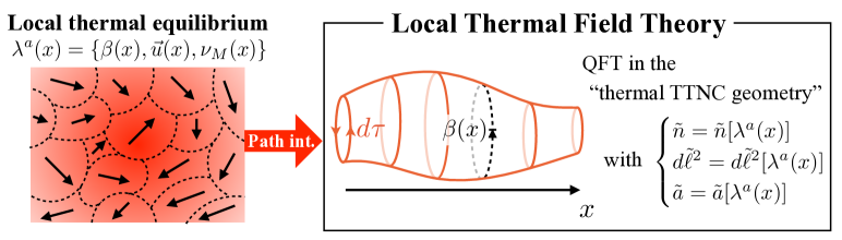
Figure 3: Schematic picture clarified in Sec. 3.2. We develop the imaginary-time path-integral formalisms for local thermal equilibrium, which brings about the emergence of the thermal twistless torsional Newton-Cartan (TTNC) geometry.

3.3 Symmetry and invariant of emergent thermal spacetime

As is obtained in the previous subsection, the path-integral formula for the Massieu-Planck functional is given by the covariant action in the thermally emergent background. As a consequence, we again encountered the Milne boost redundancy in thermal spacetime. This gauge ambiguity is not useful to construct the Massieu-Planck functional $\Psi[\bar{t};\lambda,j]$—Milne boost invariant quantity—in terms of $\tilde{j}(x)$ since some members of $\tilde{j}(x)$ are not Milne boost invariant. We thus would like to describe our background in the Milne boost invariant manner. Nevertheless, we also need to pay attention to the $U(1)_{M}$ mass gauge invariance of $\Psi[\bar{t};\lambda,j]$ since there is a kind of tradeoff between the $U(1)_{M}$ gauge invariance and Milne boost invariance. In other words, if we are not careful, our Milne boost invariant quantities may not be $U(1)_{M}$ gauge invariant, or reversed case may occur. We here explain how we can respect both of them and specify the Milne boost and $U(1)_{M}$ gauge invariant quantities employed as basic building blocks for $\Psi[\bar{t};\lambda,j]$.

We first pay attention to the $U(1)_{M}$ gauge invariance. In the usual situation, we have the field strength tensor $F^{a}\equiv d\tilde{a}$ and $F=dA$ as gauge invariant building blocks. They contain one derivative, and thus, do not appear in the leading-order expression of $\Psi[\bar{t};\lambda,j]$ when we consider the derivative expansion with a usual power counting scheme as is employed in Sec. 5. However, we have another gauge invariant quantity in our setup due to the compactness of the imaginary-time direction. In fact, following contour integrals along the imaginary-time direction (See Fig. 4) provides us a diffeormophism and $U(1)_{M}$ gauge invariant quantities:

$$\oint_{C}\tilde{n}=\oint_{0}^{\beta_{0}}d\tilde{t}e^{\sigma}=\beta(x),\quad\oint_{C}\tilde{a}=\oint_{0}^{\beta_{0}}d\tilde{t}e^{\sigma}\mu^{\prime}_{M}=\nu^{\prime}_{M}(x),$$ (97)

where we employed the gauge (86) for $\tilde{a}$. As is clearly seen, these do not contain any derivative, which can appear in the leading-order expression of $\Psi[\bar{t};\lambda,j]$. However, the second term $\nu^{\prime}_{M}(x)$ is indeed not Milne boost invariant, and we have further restriction.

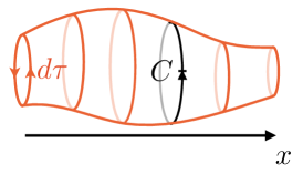
Figure 4: A contour of integral used in Eq. (97). This contour results from the compactness of thermal spacetime along the imaginary-time direction.

We then discuss how the Milne boost invariance restricts the possible combination of our building blocks. Following Ref. Jensen:2014ama , let us first construct the Milne boost invariant “line element”. The important point clarified in the previous subsection is that spatial line element $d\tilde{\ell}^{2}$ and $U(1)_{M}$ gauge connection $d\tilde{a}$ is not Milne boost invariant. However, utilizing these Milne boost covariance, we can construct the Milne boost invariant “line element” as follows:

$$\begin{split}d\tilde{s}^{2}&\equiv d\tilde{\ell}^{2}-\tilde{n}\otimes\tilde{a}-\tilde{a}\otimes n\\ &=\big{(}\tilde{h}_{\bar{\mu}\bar{\nu}}-\tilde{n}_{\bar{\mu}}\tilde{a}_{\bar{\nu}}-\tilde{a}_{\bar{\mu}}\tilde{n}_{\bar{\nu}}\big{)}d\tilde{x}^{\bar{\mu}}\otimes d\tilde{x}^{\bar{\nu}}\\ &=2e^{2\sigma}\Big{(}\mu_{M}^{\prime}+\frac{1}{2}u^{2}\Big{)}d\tilde{t}\otimes d\tilde{t}-e^{\sigma}\big{(}a_{{\bar{i}}}-u_{{\bar{i}}}\big{)}(d\tilde{t}\otimes d\tilde{x}^{{\bar{i}}}+d\tilde{x}^{{\bar{i}}}\otimes d\tilde{t})+h_{{\bar{i}}{\bar{j}}}dx^{{\bar{i}}}\otimes dx^{{\bar{j}}},\end{split}$$ (98)

from which we can read off the Milne boost invariant combinations:

$$\nu_{M}\equiv\nu_{M}^{\prime}+\frac{1}{2}\beta u^{2},\quad a^{\prime}_{{\bar{i}}}\equiv a_{{\bar{i}}}-u_{{\bar{i}}}.$$ (99)

Note that while the Milne boost invariance is respected, the $U(1)_{M}$ gauge invariance is sacrificed; in other words, $d\tilde{s}^{2}$ is Milne boost invariant but not $U(1)_{M}$ gauge invariant. However, we have already clarified the $U(1)_{M}$ gauge invariance of $\nu_{M}^{\prime}$ and covariance of $a_{{\bar{i}}}$. Therefore, in order to construct the Massieu-Planck functional, paying attention to the diffeomorphism and gauge invariance, we only need to use $\beta(x)$ and $\nu_{M}(x)=\nu_{M}^{\prime}(x)+\frac{1}{2}\beta u(x)^{2}$ as leading-order scalar quantities, $a^{\prime}_{{\bar{i}}}=a_{{\bar{i}}}-u_{{\bar{i}}}$ and $A_{{\bar{i}}}$ as gauge fields, and $h_{{\bar{i}}{\bar{j}}}$ (or $h^{{\bar{i}}{\bar{j}}}$) as a spatial metric. This restriction on building blocks of $\Psi[\bar{t};\lambda,j]$ is a basic consequence resulting from the symmetry properties, which will be effectively utilized in Sec. 5.

Before closing this section, we put a comment on the relation between the gauge choice and Milne boost invariance. In this subsection, starting from one seemingly useful gauge (86), we discuss a way to implement the Milne boost invariance. However, if we start from another gauge (90), we notice that all information on backgrounds in Eq. (93) is already Milne boost invariant. As is discussed in Ref. Jensen:2014ama , this comes from the fact that we have the Milne boost invariant vector $u^{\mu}$ which enables us to realize the Milne boost invariant gauge fixing. Therefore, from the viewpoint of the Milne boost invariance, the latter gauge (90) is the most useful gauge choice (See e.g. Jensen:2014ama for a detailed discussion).

4 Fluctuation theorems and optimized perturbation theory for time evolution

Let us consider systems in general nonequilibrium situations even far from local equilibrium in which innumerable microscopic degrees of freedom play an important role. As we emphasized in Sec. 1, hydrodynamics provides the macroscopic effective description of systems near local thermal equilibrium, and we do not know whether we can apply hydrodynamics to describe such really nonequilibrium situations. Nevertheless, almost all microscopic degrees of freedom will go away a short while later, and only conserved charge densities remains since they cannot disappear due to the conservation laws. This brings about local thermalization, after which hydrodynamics is expected to work. In this section, based on the above expectation, assuming that our initial density operator is given by the local Gibbs distribution, we provide a way to derive an exact formula for the dissipative part of constitutive relations. In Sec. 4.1, we show two kinds of the so-called fluctuation theorems for local thermal equilibrium before discussing the constitutive relation. In Sec. 4.2, we write down the exact formula for the dissipative part of constitutive relations based on the first fluctuation theorem.

4.1 Fluctuation theorems for local thermal equilibrium

We first put a most critical assumption that our initial density operator $\hat{\rho}_{0}$ takes a form of the local Gibbs distribution at initial time $\bar{t}_{0}$: $\hat{\rho}_{0}=\hat{\rho}_{\mathrm{LG}}[\bar{t}_{0};\lambda]$. Employing the Heisenberg picture, we express the average value of any Heisenberg operator $\hat{\mathcal{O}}(t)$ as $\langle\hat{\mathcal{O}}(t)\rangle\equiv\mathop{\mathrm{Tr}}\big{(}\hat{\rho}_{0}\hat{\mathcal{O}}(t)\big{)}$. Then, our problem is to derive the constitutive relations:

$$\langle\hat{\mathcal{J}}^{\mu}_{~{}a}(x)\rangle=\mathcal{J}^{\mu}_{~{}a}[\langle\hat{\mathcal{J}}^{\bar{0}}_{~{}a}\rangle].$$ (100)

Although we have fixed our initial density operator, it is inadequate to approximately evaluate the average value $\langle\hat{\mathcal{J}}^{\mu}_{~{}a}(x)\rangle=\mathop{\mathrm{Tr}}\big{(}\hat{\rho}_{\mathrm{LG}}[\bar{t}_{0};\lambda]\hat{\mathcal{J}}^{\mu}_{~{}a}(x)\big{)}$ at later time $\bar{t}~{}(>\bar{t}_{0})$. This is because we only have a set of local thermodynamic parameters $\lambda^{a}(x)\big{|}_{\bar{t}_{0}}$ at initial time $\bar{t}_{0}$ while we expect $\langle\hat{\mathcal{J}}^{\mu}_{~{}a}(x)\rangle$ at later time $\bar{t}$ is expressed by parameters at that time $\bar{t}$. We thus introduce a new set of parameters $\lambda^{a}(x)\big{|}_{\bar{t}}$ at $\bar{t}$ and reconstruct the perturbative expansion on the top of the newly introduced local Gibbs distribution $\hat{\rho}_{\mathrm{LG}}[\bar{t};\lambda]$, which is similar to the so-called optimized (or renormalized) perturbation theory. In other words, we decompose the initial density operator as

$$\begin{split}\hat{\rho}_{0}&=\exp\left(-\hat{S}[\bar{t}_{0};\lambda]\right)=\exp\left(-\hat{S}[\bar{t};\lambda]+\hat{S}[\bar{t};\lambda]-\hat{S}[\bar{t}_{0};\lambda]\right)\\ &=\exp\left(-\hat{S}[\bar{t};\lambda]\right)\hat{U}[\bar{t},\bar{t}_{0};\lambda],\end{split}$$ (101)

where we introduced

$$\hat{U}[\bar{t},\bar{t}_{0};\lambda]=T_{\tau}\exp\left(\int_{0}^{1}d\tau\hat{\Sigma}_{\tau}[\bar{t},\bar{t}_{0};\lambda]\right),$$ (102)

with the entropy production operator $\hat{\Sigma}[\bar{t},\bar{t}_{0};\lambda]\equiv\hat{S}[\bar{t},\lambda]-\hat{S}[\bar{t}_{0};\lambda]$ and $\hat{\mathcal{O}}_{\tau}\equiv e^{\tau\hat{S}[\bar{t},\lambda]}\hat{\mathcal{O}}e^{-\tau\hat{S}[\bar{t},\lambda]}$. Here $\hat{S}[\bar{t};\lambda]$ represents the entropy functional operator defined in Eqs. (50)-(51) whose local thermodynamics parameters are given by new ones $\lambda^{a}(x)\big{|}_{\bar{t}}$.

Since we do not put any condition to fix new parameters $\lambda^{a}(x)\big{|}_{\bar{t}}$, they are arbitrary at this stage. This means that if we are able to perform the exact calculation, the result does not depend on arbitrary parameters $\lambda^{a}(x)\big{|}_{\bar{t}}$. However, we cannot in general accomplish such an exact calculation, and rather perform the finite-order perturbative expansion on the top of a local Gibbs distribution with new parameters $\lambda^{a}(x)\big{|}_{\bar{t}}$. This truncation leads to the result dependent on a way to define the new parameters $\lambda^{a}(x)\big{|}_{\bar{t}}$. In the hydrodynamic description of systems, we are interested in the spacetime evolution of the conserved charge densities $\langle\hat{\mathcal{J}}^{\bar{0}}_{~{}a}(x)\rangle$. We, therefore, employ a condition like the fastest apparent convergence (FAC) in the optimized perturbation theory Stevenson:1981vj for $\langle\hat{\mathcal{J}}^{\bar{0}}_{~{}a}(x)\rangle$; that is to say, the deviation of conserved charge density is minimized, or vanish in this case: $\langle\hat{U}\delta\hat{\mathcal{J}}^{{\bar{0}}}_{~{}a}(x)\rangle^{\mathrm{LG}}_{\bar{t}}=0$. Since this condition is equivalent to

$$\langle\hat{\mathcal{J}}^{{\bar{0}}}_{~{}a}(x)\rangle\big{|}_{\bar{t}}=\langle\hat{\mathcal{J}}^{{\bar{0}}}_{~{}a}(x)\rangle^{\mathrm{LG}}_{\bar{t}},$$ (103)

it means that the new parameters $\lambda^{a}(x)\big{|}_{\bar{t}}$ is defined so as to match with local thermodynamics for a given value of conserved charge densities $\langle\hat{\mathcal{J}}^{{\bar{0}}}_{~{}a}(x)\rangle\big{|}_{\bar{t}}$. With the help of the decomposition of the density operator (101), we have a following exact identity to evaluate any Heisenberg operator $\hat{\mathcal{O}}(x)$:

$$\langle\hat{\mathcal{O}}(x)\rangle=\langle\hat{U}[\bar{t},\bar{t}_{0};\lambda]\hat{\mathcal{O}}(x)\rangle^{\mathrm{LG}}_{\bar{t}}.$$ (104)

This identity belongs to a variant of the fluctuation theorem which will play a central role to evaluate $\langle\hat{\mathcal{J}}^{\mu}_{~{}a}(x)\rangle$ and perturbatively construct the constitutive relation in the next section.

Unlike the classical systems sasa:2013 , we cannot show the second law of thermodynamics directly from Eq. (104) owing to the noncommutativity of quantum operators. However, we can derive a canonical quantum fluctuation theorem for local thermal equilibrium which contains the second law of thermodynamics as follows. For that purpose, defining a time evolution operator from initial time $\bar{t}_{0}$ to later time $\bar{t}$ under the influence of the external field $j(x)$ as $\hat{\mathcal{U}}_{j}(\bar{t},\bar{t}_{0})$ which satisfies $\hat{\mathcal{O}}(\bar{t})=\hat{\mathcal{U}}_{j}^{\dagger}(\bar{t},\bar{t}_{0})\hat{\mathcal{O}}(\bar{t}_{0})\hat{\mathcal{U}}_{j}(\bar{t},\bar{t}_{0})$, we introduce the following quantity

$$G_{F}(z;j]\equiv\mathop{\mathrm{Tr}}\left(\hat{\rho}_{0}\,\hat{\mathcal{U}}_{j}^{\dagger}(\bar{t},\bar{t}_{0})e^{iz\hat{S}_{0}[\bar{t};\lambda]}\hat{\mathcal{U}}_{j}(\bar{t},\bar{t}_{0})e^{-iz\hat{S}[\bar{t}_{0};\lambda]}\right)=\mathop{\mathrm{Tr}}\left(e^{-\hat{S}[\bar{t}_{0};\lambda]}e^{iz\hat{S}[\bar{t};\lambda]}e^{-iz\hat{S}[\bar{t}_{0};\lambda]}\right),$$ (105)

where $\hat{S}_{0}[\bar{t};\lambda]$ denotes the entropy functional operator whose operator argument is not $\bar{t}$ but $\bar{t}_{0}$. The notation $G(z;j]$ is used to clarify that $G(z;j]$ is a function of $z$ and functional of $j(x)$. As is clear from the second expression, this quantity apparently gives a generating function for entropy production $\hat{\Sigma}[\bar{t},\bar{t}_{0};\lambda]=\hat{S}[\bar{t};\lambda]-\hat{S}[\bar{t}_{0};\lambda]$ when we consider the forward time evolution in the presence of the external fields $j(x)$:

$$\langle\hat{\Sigma}[\bar{t},\bar{t}_{0};\lambda]\rangle=\frac{\partial}{i\partial z}G_{F}(z;j]\Big{|}_{z=0},\quad\langle(\hat{\Sigma}[\bar{t},\bar{t}_{0};\lambda])^{2}\rangle=\left(\frac{\partial}{i\partial z}\right)^{2}G_{F}(z;j]\Big{|}_{z=0}.$$ (106)

While the above first- and second-order relations are certainly true, if we consider the third- or more order general terms, this simple relation breaks down. Nevertheless, considering the projection measurement of the entropy production, we can regard $G_{F}(z;j]$ as the generating function for the entropy production being observed in an ensemble of the measurement. In fact, introducing the probability to observe the entropy production being $\sigma$ by the Fourier transformation of $G_{F}(\sigma;j]$:

$$P_{F}(\sigma;j]\equiv\int dze^{-iz\sigma}G_{F}(z;j],$$ (107)

we define the moments of $\sigma$ as

$$\langle\sigma^{n}\rangle_{P_{F}}\equiv\int d\sigma P_{F}(\sigma;j]\sigma^{n}=\left(\frac{\partial}{i\partial z}\right)^{n}G_{F}(z;j]\Big{|}_{z=0}.$$ (108)

Then, as is mentioned above, we can directly relate the first two moments of $\sigma$ over the probability distribution $P_{F}(\sigma;j]$ with the expectation values of the entropy operators $\hat{\Sigma}[\bar{t},\bar{t}_{0};\lambda]$ over the initial density operator $\hat{\rho}_{0}=\hat{\rho}_{\mathrm{LG}}[\bar{t}_{0};\lambda]$:

$$\langle\hat{\Sigma}[\bar{t},\bar{t}_{0};\lambda]\rangle=\langle\sigma\rangle_{P_{F}},\quad\langle(\hat{\Sigma}[\bar{t},\bar{t}_{0};\lambda])^{2}\rangle=\langle\sigma^{2}\rangle_{P_{F}},\quad\langle(\hat{\Sigma}[\bar{t},\bar{t}_{0};\lambda])^{n}\rangle\neq\langle\sigma^{n}\rangle_{P_{F}}\quad(n=3,4,\cdots).$$ (109)

In addition to $G_{F}(z;j]$, we also introduce

$$G_{B}(z;j]\equiv\mathop{\mathrm{Tr}}\left(e^{-\Theta\hat{S}[\bar{t}_{0};\lambda]\Theta^{-1}}\widetilde{\mathcal{U}}_{j}^{\dagger}e^{iz\Theta\hat{S}_{0}[\bar{t};\lambda]\Theta^{-1}}\widetilde{\mathcal{U}}_{j}e^{-iz\Theta\hat{S}[\bar{t}_{0};\lambda]\Theta^{-1}}\right),$$ (110)

where we introduced $\Theta\equiv\mathcal{P}\mathcal{T}$ with $\mathcal{P}$ and $\mathcal{T}$ represent parity and time-reversal transformation, respectively. Note that we insert $\mathcal{P}\mathcal{T}$ transformation instead of the simple time-reversal transformation usually employed in the quantum fluctuation theorem. Here $\widetilde{\mathcal{U}}_{j}$ is defined as

$$\widetilde{\mathcal{U}}_{j}\equiv\Theta\,\hat{\mathcal{U}}_{j}^{\dagger}(\bar{t},\bar{t}_{0})\Theta^{-1},$$ (111)

which represents the backward evolution, or the time-evolution with a spacetime-reversed protocol for external fields $j(x)$. Moreover, in the same way as $P_{F}(\sigma;j]$, we introduce the probability distribution of the entropy production as

$$P_{B}(\sigma;j]\equiv\int dze^{-iz\sigma}G_{B}(z;j].$$ (112)

Based on this setup, we can show the following simple identity

$$G_{F}(z;j]=G_{B}(-z+i;j],$$ (113)

which gives an extension of the canonical quantum fluctuation theorem in the case of local thermal equilibrium. The crucial assumptions to prove this identity is the local Gibbs form of the initial density operator. We put a proof of this identity in Appendix A. Here, we demonstrate some consequences from this identity. First of all, we can rewrite the quantum fluctuation theorem in an alternative form in terms of $P_{F,B}(\sigma;j]$ as follows:

$$P_{F}(\sigma;j]=e^{\sigma}P_{B}(-\sigma;j].$$ (114)

Using the above identity for $G_{F,R}(z;j]$, we can easily prove this as

$$\begin{split}P_{F}(\sigma)&=\int dze^{-iz\sigma}G_{F}(z)=\int dze^{-iz\sigma}G_{B}(-z+i)\\ &=e^{\sigma}\int dze^{iz^{\prime}\sigma}G_{B}(z^{\prime})=e^{\sigma}P_{B}(-\sigma).\end{split}$$ (115)

This identity immediately brings about the so-called the integral fluctuation theorem for local thermal equilibrium

$$\langle e^{-\sigma}\rangle_{P_{F}}\equiv\int d\sigma P_{F}(\sigma;j]e^{-\sigma}=\int d\sigma P_{B}(-\sigma;j]=1,$$ (116)

where we used the above identity for $P_{F,B}(\sigma;j]$. It is worth to emphasize that $\langle f(\sigma)\rangle_{P_{F}}\equiv\int d\sigma P_{F}(\sigma;j]f(\sigma)$ is not equal to $\langle f(\hat{\Sigma})\rangle\equiv\mathop{\mathrm{Tr}}\big{(}\hat{\rho}_{0}f(\hat{\Sigma})\big{)}$ except for the special case with the first-order or second-order terms of them due to Eq. (109). Then, taking into account Jensen’s inequality ($e^{-x}\geq-x+1$), this identity provides the following inequality

$$1=\langle e^{-\sigma}\rangle_{P_{F}}\geq-\langle\sigma\rangle_{P_{F}}+1\quad\Leftrightarrow\quad\langle\sigma\rangle_{P_{F}}=\langle\hat{\Sigma}[\bar{t},\bar{t}_{0};\lambda]\rangle\geq 0.$$ (117)

This is precisely the second law of thermodynamics which we want to show. Moreover, expanding $e^{-\sigma}$ with respect to $\sigma$ and neglecting the $O(\sigma^{3})$ terms, we can evaluate the left-hand-side of the integral fluctuation theorem as

$$\begin{split}\langle e^{-\sigma}\rangle_{P_{F}}&=1-\langle\sigma\rangle_{P_{F}}+\frac{1}{2}\langle\sigma^{2}\rangle_{P_{F}}+O(\sigma^{3})\\ &=1-\langle\hat{\Sigma}[\bar{t},\bar{t}_{0};\lambda]\rangle+\frac{1}{2}\langle(\hat{\Sigma}[\bar{t},\bar{t}_{0};\lambda])^{2}\rangle+O(\sigma^{3}),\end{split}$$ (119)

where we used Eq. (109) to proceed the second line. Therefore, we can also derive the following relation

$$\langle\hat{\Sigma}[\bar{t},\bar{t}_{0};\lambda]\rangle=\frac{1}{2}\langle(\hat{\Sigma}[\bar{t},\bar{t}_{0};\lambda])^{2}\rangle+O(\sigma^{3}),$$ (120)

which provides the relation between the dissipation (the left-hand-side) and fluctuation (the right-hand-side). Although this relation does not play a central role in our derivation of hydrodynamic equations, we can understand this as a generalization of fluctuation-dissipation relations in our setup.

4.2 Exact formula for dissipative constitutive relations

Based on the first fluctuation-like theorem obtained above, let us derive the exact formula for the dissipative part of the constitutive relations. Although there are several differences, this procedure is accomplished in the same way as the relativistic case Hayata:2015lga . First of all, the identity (104) enable us to decompose $\langle\hat{\mathcal{J}}^{\mu}_{~{}a}(x)\rangle$ into two parts

$$\langle\hat{\mathcal{J}}^{\mu}_{~{}a}(x)\rangle=\langle\hat{\mathcal{J}}^{\mu}_{~{}a}(x)\rangle^{\mathrm{LG}}_{\bar{t}}+\langle\delta\hat{\mathcal{J}}^{\mu}_{~{}a}(x)\rangle\quad\mathrm{with}\quad\langle\delta\hat{\mathcal{J}}^{\mu}_{~{}a}(x)\rangle\equiv\langle\hat{U}\delta\hat{\mathcal{J}}^{\mu}_{~{}a}(x)\rangle^{\mathrm{LG}}_{\bar{t}},$$ (121)

where we introduced $\langle\hat{\mathcal{O}}\rangle^{\mathrm{LG}}_{\bar{t}}\equiv\mathop{\mathrm{Tr}}(\hat{\rho}_{\mathrm{LG}}[\bar{t};\lambda]\hat{\mathcal{O}})$ and $\delta\hat{\mathcal{O}}\equiv\hat{\mathcal{O}}-\langle\hat{\mathcal{O}}\rangle^{\mathrm{LG}}_{\bar{t}}$. The first term—the expectation values of conserved current operators over the local Gibbs distribution—can be evaluated from the Massieu-Planck functional as discussed in the previous section. We thus focus on the second term associated with the deviation from local thermal equilibrium.

In order to evaluate the second term, we first rewrite an expression of the entropy production operator $\hat{\Sigma}[\bar{t},\bar{t}_{0};\lambda]$ staying in $\hat{U}$ as

$$\begin{split}\hat{\Sigma}[\bar{t},\bar{t}_{0};\lambda]&\equiv\hat{S}[\bar{t};\lambda]-\hat{S}[\bar{t}_{0};\lambda]\\ &=\int_{\bar{t}_{0}}^{\bar{t}}d\bar{s}\partial_{\bar{s}}\left[-\int d\Sigma_{\bar{s}\mu}\hat{\mathcal{J}}^{\mu}_{~{}a}\lambda^{a}+\Psi[\bar{s};\lambda]\right]\\ &=-\int_{\bar{t}_{0}}^{\bar{t}}d\bar{s}\int d\Sigma_{\bar{s}}N(\bar{s})\Big{[}\delta\hat{\mathcal{T}}^{\mu}_{~{}\nu}\Big{(}\nabla_{\mu}\beta^{\nu}-\beta^{\rho}(F^{n}_{\mu\rho}v^{\nu}+n_{\mu}\nabla_{\rho}v^{\nu})\Big{)}\\ &\hskip 93.0pt+\delta\hat{J}_{M}^{\mu}\big{(}\nabla_{\mu}\nu^{\prime}_{M}+\beta^{\nu}F^{a}_{\mu\nu}\big{)}+\delta\hat{J}_{Q}^{\mu}\big{(}\nabla_{\mu}\nu^{\prime}_{Q}+\beta^{\nu}F_{\mu\nu}\big{)}\Big{]}.\end{split}$$ (122)

Here we used the first line of Eq. (64) together with the identity (68) for $\partial_{\bar{t}}\Psi[\bar{t};\lambda]$, which leads to the subtraction of $\langle\hat{\mathcal{J}}^{\mu}_{~{}a}(x)\rangle^{\mathrm{LG}}_{\bar{t}}$. Defining a shorthand notation $\nabla_{\mu}\Lambda^{a}~{}(a=0,1,\cdots,d-1,d,d+1)$ as

$$\nabla_{\mu}\Lambda^{\nu}\equiv\nabla_{\mu}\beta^{\nu}-\beta^{\rho}(F^{n}_{\mu\rho}v^{\nu}+n_{\mu}\nabla_{\rho}v^{\nu}),\quad\nabla_{\mu}\Lambda^{d}\equiv\nabla_{\mu}\nu^{\prime}_{M}+\beta^{\nu}F^{a}_{\mu\nu},\quad\nabla_{\mu}\Lambda^{d+1}\equiv\nabla_{\mu}\nu^{\prime}_{Q}+\beta^{\nu}F_{\mu\nu},$$ (123)

we can express the entropy production operator in a compact form as

$$\hat{\Sigma}[\bar{t},\bar{t}_{0};\lambda]=-\int_{\bar{t}_{0}}^{\bar{t}}d\bar{s}\int d\Sigma_{\bar{s}}N\delta\hat{\mathcal{J}}^{\mu}_{~{}a}\big{(}\nabla_{\mu}\Lambda^{a}\big{)}.$$ (124)

This provides us the expression of the entropy production operator in terms of the local thermodynamic parameters $\lambda^{a}(x)$, external fields $j(x)$, and conserved current operators $\hat{\mathcal{J}}^{\mu}_{~{}a}(x)$. Nevertheless, this expression contains the time derivative of parameters $\lambda^{a}(x)$ whose time dependence is governed by the hydrodynamic equation. This means that we have the massless hydrodynamic mode which cause an undesirable behavior for correlation functions. We then eliminate them in a self-consistent manner by formally rearranging hydrodynamic equations: $(\nabla_{\mu}-\mathcal{G}_{\mu})\langle\hat{\mathcal{J}}^{\mu}_{~{}a}\rangle=\langle\hat{\mathcal{S}}_{a}\rangle$. To accomplish this, taking into account the fact that $e^{-\hat{S}[\bar{t};\lambda]}$ does not depend on spatial coordinate: $\nabla_{\perp\mu}\hat{S}[\bar{t};\lambda]=0$, we rewrite the local Gibbs part in hydrodynamic equations as

$$\begin{split}(\nabla_{\mu}-\mathcal{G}_{\mu})\langle\hat{\mathcal{J}}^{\mu}_{~{}a}(x)\rangle^{\mathrm{LG}}_{\bar{t}}&=(\nabla_{\mu}-\mathcal{G}_{\mu})\mathop{\mathrm{Tr}}\left[e^{-\hat{S}[\bar{t};\lambda]}\hat{\mathcal{J}}^{\mu}_{~{}a}(x)\right]\\ &=\mathop{\mathrm{Tr}}\left[\frac{1}{N(x)}(\partial_{\bar{t}}e^{-\hat{S}[\bar{t};\lambda]})\hat{c}_{a}(x)\right]+\langle\hat{\mathcal{S}}_{a}(x)\rangle^{\mathrm{LG}}_{\bar{t}}\\ &=-\frac{1}{N(x)}\int d\Sigma^{\prime}_{\bar{t}}N(x^{\prime})\nabla_{\mu}^{\prime}\Lambda^{b}(x^{\prime})\bm{(}{\delta\hat{c}_{a}(x),\delta\hat{\mathcal{J}}^{\mu}_{~{}b}(x^{\prime})}\bm{)}_{\bar{t}}+\langle\hat{\mathcal{S}}_{a}(x)\rangle^{\mathrm{LG}}_{\bar{t}},\end{split}$$ (125)

where we decomposed the covariant derivative as $\nabla_{\mu}=n_{\mu}v^{\nu}\nabla_{\nu}+P^{\nu}_{\mu}\nabla_{\nu}=n_{\mu}v^{\nu}\nabla_{\nu}+\nabla_{\perp\mu}$, and used conservation laws to proceed the second line. We also used the following result to evaluate the time derivative of $e^{-\hat{S}[\bar{t};\lambda]}$:

$$\begin{split}\partial_{\bar{t}}e^{-\hat{S}[\bar{t};\lambda]}&\equiv\lim_{\Delta\bar{t}\to 0}\frac{e^{-\hat{S}[\bar{t}+\Delta\bar{t};\lambda]}-e^{-\hat{S}[\bar{t};\lambda]}}{\Delta\bar{t}}\\ &=\lim_{\Delta\bar{t}\to 0}\frac{e^{-\hat{S}[\bar{t};\lambda]}(T_{\tau}e^{-\int_{0}^{1}d\tau\hat{\Sigma}_{\tau}[\bar{t},\bar{t}+\Delta\bar{t};\lambda]}-1)}{\Delta\bar{t}}\\ &=-e^{-\hat{S}[\bar{t};\lambda]}T_{\tau}\int_{0}^{1}d\tau\int d\Sigma^{\prime}_{\bar{t}}N(x^{\prime})\nabla_{\mu}^{\prime}\Lambda^{a}(x^{\prime})e^{\tau\hat{K}[\bar{t};\lambda]}\delta\hat{\mathcal{J}}^{\mu}_{~{}a}(x^{\prime})e^{-\tau\hat{K}[\bar{t};\lambda]}.\end{split}$$ (126)

Therefore, introducing the time-dependent local Gibbs version of the Kubo-Mori-Bogoliubov inner product $\bm{(}{\hat{A},\hat{B}}\bm{)}_{\bar{t}}$ as

$$\bm{(}{\hat{A},\hat{B}}\bm{)}_{\bar{t}}\equiv\int_{0}^{1}d\tau\langle e^{\hat{K}[\lambda;\bar{t}]\tau}\hat{A}e^{-\hat{K}[\lambda;\bar{t}]\tau}\hat{B}^{\dagger}\rangle^{\mathrm{LG}}_{\bar{t}},$$ (127)

we can rewrite the full hydrodynamic equation $(\nabla_{\mu}-\mathcal{G}_{\mu})\langle\hat{\mathcal{J}}^{\mu}_{~{}a}(x)\rangle=(\nabla_{\mu}-\mathcal{G}_{\mu})\langle\hat{\mathcal{J}}^{\mu}_{~{}a}(x)\rangle^{\mathrm{LG}}+(\nabla_{\mu}-\mathcal{G}_{\mu})\langle\delta\hat{\mathcal{J}}^{\mu}_{~{}a}\rangle=\langle\hat{\mathcal{S}}_{a}(x)\rangle$ in the following form:

$$\begin{split}&\quad\int d\Sigma^{\prime}_{\bar{t}}\bm{(}{\delta\hat{c}_{a}(x),\delta\hat{c}_{b}(x^{\prime})}\bm{)}_{\bar{t}}N(x^{\prime})\nabla_{\bar{t}}^{\prime}\Lambda^{b}(x^{\prime})\\ &+\int d\Sigma^{\prime}_{\bar{t}}\bm{(}{\delta\hat{c}_{a}(x),\delta\hat{\mathcal{J}}^{\mu}_{~{}b}(x^{\prime})}\bm{)}_{\bar{t}}N(x^{\prime})\nabla_{\perp\mu}^{\prime}\Lambda^{b}(x^{\prime})=N(x)\left[(\nabla_{\mu}-\mathcal{G}_{\mu})\langle\delta\hat{\mathcal{J}}^{\mu}_{~{}b}\rangle-\langle\delta\hat{\mathcal{S}}_{b}(x)\rangle\right].\end{split}$$ (128)

Noting that we have a generalized susceptibility $\chi_{ab}(x,x^{\prime};\bar{t})\equiv\bm{(}{\delta\hat{c}_{a}(x),\delta\hat{c}_{b}(x^{\prime})}\bm{)}_{\bar{t}}$ in front of the time derivatives in the first term, we multiply the its inverse $\chi^{ab}(x,x^{\prime};\bar{t})\equiv\bm{(}{\delta\hat{c}_{a}(x),\delta\hat{c}_{b}(x^{\prime})}\bm{)}_{\bar{t}}^{-1}$ and integrate with respect to the spatical coordinate $x^{\prime}$, which results in

$$\begin{split}N(x)\nabla_{\bar{t}}\Lambda^{a}(x)&=-\int d\Sigma^{\prime}_{\bar{t}}\int d\Sigma^{\prime\prime}_{\bar{t}}\bm{(}{\delta\hat{c}_{a}(x),\delta\hat{c}_{b}(x^{\prime})}\bm{)}_{\bar{t}}^{-1}\bm{(}{\delta\hat{c}_{b}(x^{\prime}),\delta\hat{\mathcal{J}}^{\mu}_{~{}c}(x^{\prime\prime})}\bm{)}_{\bar{t}}N(x^{\prime\prime})\nabla_{\perp\mu}^{\prime\prime}\Lambda^{c}(x^{\prime\prime})\\ &\quad+\int d\Sigma^{\prime}_{\bar{t}}\bm{(}{\delta\hat{c}_{a}(x),\delta\hat{c}_{b}(x^{\prime})}\bm{)}_{\bar{t}}^{-1}N(x^{\prime})\left[(\nabla^{\prime}_{\mu}-\mathcal{G}_{\mu})\langle\delta\hat{\mathcal{J}}^{\mu}_{~{}b}(x^{\prime})\rangle-\langle\delta\hat{\mathcal{S}}_{b}(x^{\prime})\rangle\right].\end{split}$$ (129)

This equation enables us to eliminate the time derivative from the entropy production operator (124). It is then natural and convenient to introduce the projection operator $\hat{\mathcal{P}}$ onto $\delta\hat{c}_{a}$ used in Refs. PhysRevA.8.2048 ; Hayata:2015lga ; Esposito1994 by

$$\hat{\mathcal{P}}\hat{\mathcal{O}}\equiv\int d\Sigma_{\bar{t}}\int d\Sigma_{\bar{t}}^{\prime}\delta\hat{c}_{a}(x)\bm{(}{\delta\hat{c}_{a}(x),\delta\hat{c}_{b}(x^{\prime})}\bm{)}_{\bar{t}}^{-1}\bm{(}{\delta\hat{c}_{b}(x^{\prime}),\hat{\mathcal{O}}}\bm{)}_{\bar{t}}.$$ (130)

When our system is in global thermal equilibrium, this projection operator reduces to the so-called Mori’s projection operator Mori2 . As is mentioned above, $\bm{(}{\delta\hat{c}_{a}(x),\delta\hat{c}_{b}(x^{\prime})}\bm{)}_{\bar{t}}$ is the generalized susceptibility given by

$$\chi_{ab}(x,x^{\prime};\bar{t})\equiv\bm{(}{\delta\hat{c}_{a}(x),\delta\hat{c}_{b}(x^{\prime})}\bm{)}_{\bar{t}}=\frac{\delta c_{b}(x^{\prime})}{\delta\lambda^{a}(x)}=\frac{\delta^{2}\Psi[\bar{t};\lambda,j]}{\delta\lambda^{a}(x)\delta\lambda^{b}(x^{\prime})},$$ (131)

which brings about the following expression of the inverse generalized susceptibility:

$$\chi^{ab}(x,x^{\prime};\bar{t})\equiv\bm{(}{\delta\hat{c}_{a}(x),\delta\hat{c}_{b}(x^{\prime})}\bm{)}_{\bar{t}}^{-1}=\frac{\delta\lambda^{b}(x^{\prime})}{\delta c_{a}(x)}=-\frac{\delta^{2}S[\bar{t};c]}{\delta c_{a}(x)\delta c_{b}(x^{\prime})},$$ (132)

where the second expressions of Eqs. (131)-(132) are due to Eqs. (53) and (57). This expression for the inverse susceptibility together with

$$\bm{(}{\delta\hat{c}_{b}(x^{\prime}),\hat{\mathcal{O}}}\bm{)}_{\bar{t}}=\frac{\delta}{\delta\lambda^{b}(x^{\prime})}\langle\hat{\mathcal{O}}\rangle^{\mathrm{LG}}_{\bar{t}},$$ (133)

allows us to rewrite the projection operator in a more explicit form as

$$\hat{\mathcal{P}}\hat{\mathcal{O}}=\int d\Sigma_{\bar{t}}\int d\Sigma_{\bar{t}}^{\prime}\delta\hat{c}_{a}(x)\frac{\delta\lambda^{b}(x^{\prime})}{\delta c_{a}(x)}\frac{\delta}{\delta\lambda^{b}(x^{\prime})}\langle\hat{\mathcal{O}}\rangle^{\mathrm{LG}}_{\bar{t}}=\int d\Sigma_{\bar{t}}\delta\hat{c}_{a}(x)\frac{\delta}{\delta c_{a}(x)}\langle\hat{\mathcal{O}}\rangle^{\mathrm{LG}}_{\bar{t}},$$ (134)

from which we can clearly see that $\hat{\mathcal{P}}$ gives the projection of an arbitrary operator $\hat{\mathcal{O}}$ onto $\delta c_{a}$. As is clear from the definition (130), $\delta\hat{c}_{a}(x)$ is invariant under the operation of the projection: $\hat{\mathcal{P}}\delta\hat{c}_{a}(x)=\delta\hat{c}_{a}(x)$. With the help of this projection operator, we can compactly express $\hat{\Sigma}[\bar{t},\bar{t}_{0};\lambda]$ as

$$\begin{split}\hat{\Sigma}[\bar{t},\bar{t}_{0};\lambda]&=-\int_{\bar{t}_{0}}^{\bar{t}}d\bar{s}\int d\Sigma_{\bar{s}}N\left[(1-\hat{\mathcal{P}})\delta\hat{\mathcal{J}}^{\mu}_{~{}a}\nabla_{\perp\mu}\Lambda^{a}+\delta\hat{\lambda}^{b}\left((\nabla_{\mu}-\mathcal{G}_{\mu})\langle\delta\hat{\mathcal{J}}^{\mu}_{~{}b}\rangle-\langle\delta\hat{\mathcal{S}}_{b}\rangle\right)\right]\\ &=-\int_{\bar{t}_{0}}^{\bar{t}}d\bar{s}\int d\Sigma_{\bar{s}}N\left[\tilde{\delta}\hat{\mathcal{J}}^{\mu}_{~{}a}\nabla_{\perp\mu}\Lambda^{a}+\delta\hat{\lambda}^{b}\left((\nabla_{\mu}-\mathcal{G}_{\mu})\langle\tilde{\delta}\hat{\mathcal{J}}^{\mu}_{~{}b}\rangle-\langle\tilde{\delta}\hat{\mathcal{S}}_{b}\rangle\right)\right]\\ &=-\int_{\bar{t}_{0}}^{\bar{t}}d\bar{s}\int d\Sigma_{\bar{s}}N\Big{[}\tilde{\delta}\hat{\mathcal{T}}^{\mu}_{~{}\nu}(\nabla_{\perp\mu}\beta^{\nu}-\beta^{\sigma}F^{n}_{\rho\sigma}P_{\mu}^{\rho}v^{\nu})+\tilde{\delta}\hat{J}_{M}^{\mu}(\nabla_{\perp\mu}\nu^{\prime}_{M}+\beta^{\sigma}F^{a}_{\rho\sigma}P_{\mu}^{\rho})\\ &\hskip 80.0pt+\tilde{\delta}\hat{J}_{Q}^{\mu}(\nabla_{\perp\mu}\nu^{\prime}_{Q}+\beta^{\sigma}F_{\rho\sigma}P_{\mu}^{\rho})+\delta\hat{\lambda}^{b}\left((\nabla_{\mu}-\mathcal{G}_{\mu})\langle\tilde{\delta}\hat{\mathcal{J}}^{\mu}_{~{}b}\rangle-\langle\tilde{\delta}\hat{\mathcal{S}}_{b}\rangle\right)\Big{]}.\end{split}$$ (135)

where we defined $\tilde{\delta}\hat{\mathcal{J}}^{\mu}_{~{}a}\equiv(1-\hat{\mathcal{P}})\delta\hat{\mathcal{J}}^{\mu}_{~{}a}$ and introduced the operator $\delta\hat{\lambda}^{a}(x)$ by

$$\delta\hat{\lambda}^{a}(x)\equiv\int d\Sigma_{\bar{t}}^{\prime}\delta\hat{c}_{b}(x^{\prime})\bm{(}{\delta\hat{c}_{b}(x^{\prime}),\delta\hat{c}_{a}(x)}\bm{)}_{\bar{t}}^{-1}=\int d\Sigma_{\bar{t}}^{\prime}\delta\hat{c}_{b}(x^{\prime})\frac{\delta\lambda^{a}(x)}{\delta c_{b}(x^{\prime})}.$$ (136)

Recalling the consequence followed from the Milne boost invariance (48), the mass current $\hat{J}_{M}^{\mu}(x)$ is related to the conserved momentum density $\hat{\mathcal{P}}_{\mu}(x)$ by $\hat{\mathcal{P}}_{\mu}=h_{\mu\nu}\hat{J}_{M}^{\nu}$. Then, the trivial projection $\hat{\mathcal{P}}\delta\hat{c}_{a}(x)=\delta\hat{c}_{a}(x)$, or $\tilde{\delta}\hat{c}_{a}(x)=0$ results in a disappearance of the mass current $\hat{J}_{M}^{\mu}(x)$ from the entropy production operator: $\tilde{\delta}\hat{J}_{M}^{\mu}(x)=0$. Inserting the definition of the nonrelativistic energy-momentum tensor (44) and rearranging the integrand, we obtain

$$\begin{split}\hat{\Sigma}[\bar{t},\bar{t}_{0};\lambda]&=-\int_{\bar{t}_{0}}^{\bar{t}}d\bar{s}\int d\Sigma_{\bar{s}}N\Big{[}-\tilde{\delta}\hat{\mathcal{E}}^{\mu}(\nabla_{\perp\mu}\beta-\beta^{\sigma}F^{n}_{\rho\sigma}P_{\mu}^{\rho})+\tilde{\delta}\hat{T}_{\mu\nu}\nabla_{\perp}^{\mu}\beta^{\nu}+\tilde{\delta}\hat{J}_{Q}^{\mu}(\nabla_{\perp\mu}\nu^{\prime}_{Q}+\beta^{\sigma}F_{\rho\sigma}P_{\mu}^{\rho})\\ &\hskip 80.0pt+\delta\hat{\lambda}^{b}\left((\nabla_{\mu}-\mathcal{G}_{\mu})\langle\tilde{\delta}\hat{\mathcal{J}}^{\mu}_{~{}b}\rangle-\langle\tilde{\delta}\hat{\mathcal{S}}_{b}\rangle\right)\Big{]}.\end{split}$$ (137)

As a last step, we perform the tensor decomposition of the stress tensor $\hat{T}_{\mu\nu}$ as

$$\tilde{\delta}\hat{T}_{\mu\nu}=h_{\mu\nu}\tilde{\delta}\hat{p}+\tilde{\delta}\hat{\pi}_{\mu\nu},\quad\mathrm{with}\quad\tilde{\delta}\hat{p}\equiv\frac{1}{d-1}h^{\mu\nu}\tilde{\delta}\hat{T}_{\mu\nu},\quad\tilde{\delta}\hat{\pi}_{\mu\nu}\equiv P_{\mu}^{\rho}P_{\nu}^{\sigma}\tilde{\delta}\hat{T}_{\rho\sigma}-\frac{h_{\mu\nu}}{d-1}h^{\rho\sigma}\tilde{\delta}\hat{T}_{\rho\sigma},$$ (138)

where $\tilde{\delta}\hat{p}$ denotes the trace part and $\tilde{\delta}\hat{\pi}_{\mu\nu}$ the symmetric traceless part of the stress-tensor. We eventually obtain the following expression for the entropy production operator

$$\begin{split}\hat{\Sigma}[\bar{t},\bar{t}_{0};\lambda]&=\int_{\bar{t}_{0}}^{\bar{t}}d\bar{s}\int d\Sigma_{\bar{t}}N\Big{[}\tilde{\delta}\hat{\mathcal{E}}^{\mu}(\nabla_{\perp\mu}\beta-\beta^{\sigma}P_{\mu}^{\rho}F^{n}_{\rho\sigma})-\tilde{\delta}\hat{p}(h_{\mu\nu}\nabla_{\perp}^{\mu}\beta^{\nu})-\tilde{\delta}\hat{\pi}_{\mu\nu}\nabla_{\perp}^{\langle\mu}\beta^{\nu\rangle}\\ &\hskip 70.0pt-\tilde{\delta}\hat{J}_{Q}^{\mu}(\nabla_{\perp\mu}\nu^{\prime}_{Q}+\beta^{\sigma}P_{\mu}^{\rho}F_{\rho\sigma})-\delta\hat{\lambda}^{a}\left((\nabla_{\mu}-\mathcal{G}_{\mu})\langle\tilde{\delta}\hat{\mathcal{J}}^{\mu}_{~{}a}\rangle-\langle\tilde{\delta}\hat{\mathcal{S}}_{a}\rangle\right)\Big{]},\end{split}$$ (139)

where we defined the symmetric traceless projection of $\nabla^{\mu}\beta^{\nu}$ as

$$\nabla^{\langle\mu}\beta^{\nu\rangle}\equiv\frac{1}{2}P_{\rho}^{\mu}P_{\sigma}^{\nu}(\nabla^{\rho}\beta^{\sigma}+\nabla^{\sigma}\beta^{\rho})-\frac{h^{\mu\nu}}{d-1}h_{\rho\sigma}\nabla^{\rho}\beta^{\sigma}.$$ (140)

Here we note that $\nabla_{\mu}\langle\tilde{\delta}\hat{\mathcal{J}}^{\mu}_{~{}a}\rangle$ does not contain the explicit time derivative because we have

$$\nabla_{\mu}\langle\tilde{\delta}\hat{\mathcal{J}}^{\mu}_{~{}a}\rangle=(n_{\mu}v^{\nu}\nabla_{\nu}+\nabla_{\perp\mu})\langle\tilde{\delta}\hat{\mathcal{J}}^{\mu}_{~{}a}\rangle=\big{(}-(v^{\nu}\nabla_{\nu}n_{\mu})+\nabla_{\perp\mu}\big{)}\langle\tilde{\delta}\hat{\mathcal{J}}^{\mu}_{~{}a}\rangle=\nabla_{\perp\mu}\langle\tilde{\delta}\hat{\mathcal{J}}^{\mu}_{~{}a}\rangle,$$ (141)

where we used the derivative of $n_{\mu}\langle\tilde{\delta}\hat{\mathcal{J}}^{\mu}_{~{}a}\rangle=\langle\tilde{\delta}\hat{c}_{a}\rangle=0$ for the second equality and compatibility condition $\nabla_{\nu}n_{\mu}=0$ for the last equality. Therefore, the entropy production operator (139) is written in terms of the external fields $j(x)$ and the spatial derivative of local thermodynamic parameters $\lambda^{a}(x)$. However, we also note that the time derivative of parameters may appear from the higher-order correction of $\langle\tilde{\delta}\hat{\mathcal{J}}^{\mu}_{~{}a}\rangle$.

Then, noting $\langle\delta\hat{\mathcal{J}}^{\mu}_{~{}a}(x)\rangle=\langle\tilde{\delta}\hat{\mathcal{J}}^{\mu}_{~{}a}(x)\rangle$ due to $\langle\delta\hat{c}_{a}(x)\rangle=0$ followed from our condition to determine local thermodynamic parameters (103), we eventually obtain the final expression for $\langle\delta\hat{\mathcal{J}}^{\mu}_{~{}a}\rangle$ as

$$\langle\delta\hat{\mathcal{J}}^{\mu}_{~{}a}(x)\rangle=\langle T_{\tau}e^{\int_{0}^{1}d\tau\hat{\Sigma}_{\tau}[\bar{t},\bar{t}_{0};\lambda]}\tilde{\delta}\hat{\mathcal{J}}^{\mu}_{~{}a}(x)\rangle^{\mathrm{LG}}_{\bar{t}}.$$ (142)

This equation together with the expression of the entropy production operator (139) provides an exact formula for the dissipative part of the constitutive relations. Since $\hat{\Sigma}_{\tau}[\bar{t},\bar{t}_{0};\lambda]$ contains $\langle\tilde{\delta}\hat{\mathcal{J}}^{\mu}_{~{}a}(x)\rangle$, the above equation gives a self-consistent equation to determine $\langle\tilde{\delta}\hat{\mathcal{J}}^{\mu}_{~{}a}(x)\rangle$, which can be solved order-by-order with respect to the derivative expansion of $\lambda^{a}(x)$ as discussed in the next section.

5 Derivation of hydrodynamic equations

In this section, based on the exact formulae derived in the previous sections, we perform the derivative expansion and derive hydrodynamic equations order-by-order. We restrict ourselves to the simplest case—a single component parity-even fluid in the zeroth-order and first-order derivative expansion. As a consequence, we obtain the constitutive relations for the perfect fluid and Navier-Stokes fluid, respectively. After demonstrating our basic procedure, we give the leading-order (zeroth-order) result in Sec. 5.1. In Sec. 5.2, we proceed to the first-order correction to the constitutive relation, which leads to the Navier-Stokes equation.

Before starting the discussion, we briefly summarize our starting point for the derivative expansion. The result obtained so far is summarized as follows: We have decomposed the full average of conserved current operators into two parts:

$$\langle\hat{\mathcal{J}}^{\mu}_{~{}a}(x)\rangle=\langle\hat{\mathcal{J}}^{\mu}_{~{}a}(x)\rangle^{\mathrm{LG}}_{\bar{t}}+\langle\delta\hat{\mathcal{J}}^{\mu}_{~{}a}(x)\rangle.$$ (143)

Here the first term represents the nondissipative part appearing in local thermal equilibrium and the second terms does the dissipative part originated from the derivation from local thermal equilibrium. We have derived the exact formulae for both of them as given in Eqs. (66), or (73) in the hydrostatic gauge, and Eq. (142).

Therefore, in order to evaluate the nondissipative part of constitutive relation order-by-order, we only need to perform the derivative expansion of the Massieu-Planck functional $\Psi[\bar{t};\lambda,j]$. For that purpose, we have to specify a power counting scheme for the parameters such as $\lambda^{a}(x)$, and external fields $j(x)$. We employ the most standard choice in this paper where all parameters are order $p^{0}$: $\lambda^{a}=j=O(p^{0})$, which allow us to apply the usual derivative expansion. Here we use the momentum $p$ instead of the spatial derivative $\nabla_{\perp}$. Nevertheless, note that this is not the unique choice since we should adopt other power counting scheme to describe systems e.g. in the presence of the strong magnetic field. Since we fix our power counting scheme, based on the symmetry arguments, we can perform the derivative expansion of the Massieu-Planck functional as

$$\Psi[\bar{t};\lambda,j]=\Psi^{(0)}[\bar{t};\lambda,j]+\Psi^{(1)}[\bar{t};\lambda,j]+\Psi^{(2)}[\bar{t};\lambda,j]+\cdots,$$ (144)

which provides nondissipative constitutive relations for $\langle\hat{\mathcal{J}}^{\mu}_{~{}a}(x)\rangle^{\mathrm{LG}}_{\bar{t}}$. Here upper indices in the right-hand side of this equation denotes the number of the spatial derivative (or momentum $p$). Note that we only have the spatial derivative due to the definition of the Massieu-Planck functional.

Furthermore, expanding $\hat{U}$ in Eq. (142) together with the entropy production operator (139) provides us the dissipative part of constitutive relations in a self-consistent manner. Since the entropy functional inescapably contain at least one spatial derivative of parameters, the expansion with respect to $\hat{\Sigma}$ can be regarded as the derivative expansion. We then obtain

$$\begin{split}\langle\tilde{\delta}\hat{\mathcal{J}}^{\mu}_{~{}a}(x)\rangle&=\langle T_{\tau}e^{\int_{0}^{1}d\tau\hat{\Sigma}_{\tau}[\bar{t},\bar{t}_{0};\lambda]}\tilde{\delta}\hat{\mathcal{J}}^{\mu}_{~{}a}(x)\rangle^{\mathrm{LG}}_{\bar{t}}\\ &=\langle\tilde{\delta}\hat{\mathcal{J}}^{\mu}_{~{}a}(x)\rangle^{\mathrm{LG}}_{\bar{t}}+\int_{0}^{1}d\tau\langle T_{\tau}\hat{\Sigma}_{\tau}[\bar{t},\bar{t}_{0};\lambda]\tilde{\delta}\hat{\mathcal{J}}^{\mu}_{~{}a}(x)\rangle^{\mathrm{LG}}_{\bar{t}}\\ &\hskip 65.0pt+\frac{1}{2}\int_{0}^{1}d\tau\int_{0}^{1}d\tau^{\prime}\langle T_{\tau}\hat{\Sigma}_{\tau}[\bar{t},\bar{t}_{0};\lambda]\hat{\Sigma}_{\tau^{\prime}}[\bar{t},\bar{t}_{0};\lambda]\tilde{\delta}\hat{\mathcal{J}}^{\mu}_{~{}a}(x)\rangle^{\mathrm{LG}}_{\bar{t}}+\cdots.\end{split}$$ (145)

Here the first term in the second line vanish by definition: $\langle\tilde{\delta}\hat{\mathcal{J}}^{\mu}_{~{}a}(x)\rangle^{\mathrm{LG}}_{\bar{t}}=\langle\delta\hat{\mathcal{J}}^{\mu}_{~{}a}(x)\rangle^{\mathrm{LG}}_{\bar{t}}=0$. Then, the leading-order dissipative correction appears with at least one spatial derivative. Although we do not discuss the next-leading-order dissipative correction, we note that second-order corrections also arises from the second term with the single $\hat{\Sigma}_{\tau}$ in addition to contributions from the third term.

5.1 Zeroth-order result: Perfect fluid

As is clarified above, dissipative corrections to constitutive relations are inevitably accompanied by at least on spatial derivative of local thermodynamic parameters $\lambda^{a}(x)$. We, therefore, do not have the zeroth-order dissipative corrections, and we only need to evaluate the Massieu-Planck functional in the leading-order derivative expansion.

As is elaborated in Sec. 3.3, we can only use $\beta(x)$ and $\nu_{M}$ as basic building blocks of the leading-order Massieu-Planck functional $\Psi^{(0)}[\bar{t};\lambda,j]$. Then, the most general form of $\Psi^{(0)}[\bar{t};\lambda,j]$ respecting diffeomorphism and $U(1)_{M}$ gauge invariance in emergent thermal spacetime is given by

$$\Psi^{(0)}[\bar{t};\lambda]=\int_{0}^{\beta_{0}}d^{d}\tilde{x}\sqrt{\tilde{\gamma}}p(\beta,\nu_{M})=\int d^{d-1}\bar{x}\sqrt{h}\beta p(\beta,\nu_{M}),$$ (146)

where we used $\sqrt{\tilde{\gamma}}=e^{\sigma}\sqrt{h}$ with $e^{\sigma(x)}=\beta(x)/\beta_{0}$ and performed the integration with respect to $\tilde{t}$ to derive the right-hand side of this equation. Here $p(\beta,\nu_{M})$ represent a certain function dependent on $\beta$ and $\nu_{M}$ which satisfies a following relation,

$$d(\beta p)=c_{a}d\lambda^{a}=p_{\mu}d\beta^{\mu}+n_{M}d\nu_{M}^{\prime},$$ (147)

due to the thermodynamic properties of the Massieu-Planck functional (53). From this equation, we can read off its relations to the conserved charge densities as

$$\frac{\partial p}{\partial\beta}=-\frac{1}{\beta}\left(n_{\mu}\mathcal{E}^{\mu}+p+\frac{1}{2}n_{M}u^{2}\right),\quad\frac{\partial p}{\partial\nu_{M}}=\frac{n}{\beta},$$ (148)

whese we used $\beta=\beta^{\mu}n_{\mu}$, $\nu_{M}=\nu_{M}^{\prime}+\dfrac{1}{2}\beta u^{2}$, and $p_{\mu}v^{\mu}=-n_{\mu}\mathcal{E}^{\mu}$ with $\mathcal{E}^{\mu}\equiv\langle\hat{\mathcal{E}}^{\mu}\rangle^{\mathrm{LG}}_{\bar{t}}$.

Since we have obtained the explicit form of the leading-order Massieu-Planck functional $\Psi^{(0)}[\bar{t};\lambda]$, the variational formulae (66) enables us to obtain the corresponding leading-order constitutive relations. However, we further simplify the problem by employing the hydrostatic gauge developed in Sec. 3.1.2, and use the corresponding variational formulae (73). In the hydrostatic gauge, recalling the gauge fixing condition (69), we have $N(x)\big{|}_{\mathrm{hs}}\equiv n_{\mu}(x)t^{\mu}(x)\big{|}_{\mathrm{hs}}=n_{\mu}(x)\beta^{\mu}(x)/\beta_{0}=e^{\sigma}$, which leads to $\sqrt{\gamma}\big{|}_{\mathrm{hs}}=\sqrt{\tilde{\gamma}}$. Thus, we can simply express $\Psi^{(0)}[\bar{t};\lambda]$ by the use of the original background field $j(x)\big{|}_{\mathrm{hs}}$:

$$\Psi^{(0)}[\bar{t};\lambda]\big{|}_{\mathrm{hs}}=\int_{0}^{\beta_{0}}d^{d}\tilde{x}\sqrt{\gamma}p(\beta,\nu_{M})=\beta_{0}\int d^{d-1}\bar{x}\sqrt{\gamma}p(\beta,\nu_{M})\big{|}_{\mathrm{hs}}.$$ (149)

Let us then take the variation of $\Psi^{(0)}[\bar{t};\lambda]\big{|}_{\mathrm{hs}}$ with respect to the independent background fields ${\bar{j}}(x)\equiv\{n_{\mu},{\bar{v}}^{\mu},{\bar{h}}^{\mu\nu},v^{\mu},a_{\mu}\}$. For that purpose, we use a following variational formulae

$$\begin{split}\delta\beta&=\beta^{\mu}\delta n_{\mu},\\ \delta\sqrt{\gamma}&=\sqrt{\gamma}\Big{(}v^{\mu}\delta n_{\mu}-\frac{1}{2}h_{\mu\nu}\delta{\bar{h}}^{\mu\nu}\Big{)},\\ \delta\nu_{M}\big{|}_{\mathrm{hs}}&=-\beta^{\mu}\delta a_{\mu}+\frac{1}{2}u^{2}\beta^{\mu}\delta n_{\mu}-\beta u_{\mu}\delta{\bar{v}}^{\mu}-\frac{1}{2}\beta u_{\mu}u_{\nu}\delta{\bar{h}}^{\mu\nu},\end{split}$$ (150)

where we used $\nu_{M}\big{|}_{\mathrm{hs}}=-\beta^{\mu}a_{\mu}+\dfrac{1}{2}\beta u^{2}$. By using these relations, we can calculate the variation of the leading-order Massieu-Planck functional as follows:

$$\begin{split}\delta\Psi^{(0)}[\bar{t};\lambda]\big{|}_{\mathrm{hs}}&=\beta_{0}\int d^{d-1}\bar{x}\left[p\delta\sqrt{\gamma}+\frac{\partial p}{\partial\beta}\delta\beta+\frac{\partial p}{\partial\nu_{M}}\delta\nu_{M}\big{|}_{\mathrm{hs}}\right]\\ &=-\beta_{0}\int d^{d-1}\bar{x}\sqrt{\gamma}\Bigg{[}\Big{(}(\mathcal{E}\cdot n)u^{\mu}+pP^{\mu}_{\nu}u^{\mu}\Big{)}\delta n_{\mu}\\ &\hskip 90.0pt+n_{M}u_{\mu}\delta{\bar{v}}^{\mu}+\frac{1}{2}\Big{(}n_{M}u_{\mu}u_{\nu}+ph_{\mu\nu}\Big{)}\delta{\bar{h}}^{\mu\nu}+n_{M}u^{\mu}\delta a_{\mu}\Bigg{]}.\end{split}$$ (151)

Recalling the variational formulae in the hydrostatic gauge (73), we eventually obtain

$$\langle\hat{\mathcal{E}}^{\mu}(x)\rangle^{\mathrm{LG}}_{\bar{t}} =-\dfrac{1}{\beta_{0}\sqrt{\gamma}}\dfrac{\delta\Psi[\bar{t};j]}{\delta n_{\mu}(x)}\Bigg{|}_{\mathrm{hs}}=\big{(}\mathcal{E}\cdot n\big{)}u^{\mu}+pP^{\mu}_{\nu}u^{\nu},$$ (152)

$$\langle\hat{\mathcal{P}}_{\mu}(x)\rangle^{\mathrm{LG}}_{\bar{t}} =-\dfrac{1}{\beta_{0}\sqrt{\gamma}}\dfrac{\delta\Psi[\bar{t};j]}{\delta{\bar{v}}^{\mu}(x)}\Bigg{|}_{\mathrm{hs}}=n_{M}u_{\mu},$$ (153)

$$\langle\hat{T}_{\mu\nu}(x)\rangle^{\mathrm{LG}}_{\bar{t}} =-\dfrac{2}{\beta_{0}\sqrt{\gamma}}\dfrac{\delta\Psi[\bar{t};j]}{\delta{\bar{h}}^{\mu\nu}(x)}\Bigg{|}_{\mathrm{hs}}=n_{M}u_{\mu}u_{\nu}+ph_{\mu\nu},$$ (154)

$$\langle\hat{J}_{M}^{\mu}(x)\rangle^{\mathrm{LG}}_{\bar{t}} =-\dfrac{1}{\beta_{0}\sqrt{\gamma}}\frac{\delta\Psi[\bar{t};j]}{\delta a_{\mu}(x)}\Bigg{|}_{\mathrm{hs}}=n_{M}u^{\mu}.$$ (155)

These equation provide the leading-order constitutive relation which correctly reproduces the equation of motion for a perfect fluid in conjunction with the conservation laws. From these equations, we see that $p$ and $u^{\mu}$ is simply regarded as a pressure and velocity of the fluid, respectively. Combination of Eqs. (152)-(154) gives the leading-order expression for the nonrelativistic energy-momentum tensor as

$$\begin{split}\langle\hat{\mathcal{T}}^{\mu}_{~{}\nu}(x)\rangle^{\mathrm{LG}}_{\bar{t}}&=-\Big{(}\big{(}\mathcal{E}\cdot n\big{)}u^{\mu}+pP^{\mu}_{\rho}u^{\rho}\Big{)}n_{\nu}+n_{M}v^{\mu}u_{\nu}+n_{M}P^{\mu}_{\rho}u^{\rho}u_{\nu}+pP^{\mu}_{\nu}\\ &=-\big{(}\mathcal{E}\cdot n\big{)}u^{\mu}n_{\nu}+n_{M}u^{\mu}u_{\nu}+p(\delta^{\mu}_{\nu}-u^{\mu}n_{\nu}).\end{split}$$ (156)

Note that the fluid pressure in Eq. (146) can be, in principle, calculable from the microscopic quantum theory by evaluating the path-integral formula (95). Therefore, we have derived a universal form of the leading-order constitutive relations together with a way to calculate its all contents. This provides the leading-order answer to our question to derive nonrelativistic hydrodynamics raised in Sec. 1.

5.2 First-order result: Navier-Stokes fluid

Let us proceed the first-order derivative expansion and derive the constitutive relation for the Navier-Stokes fluid. First of all, it is important to notice that we do not have the first-order nondissipative correction since we are now considering systems with parity symmetry, which leads to $\Psi^{(1)}[\bar{t};\lambda,j]=0$. Thus, the nondissipative part is the same as the leading-order results (152)-(155), and we only need to take into account the leading-order dissipative corrections in the first-order derivative expansion.

In order to derive the first-order dissipative correction, we first rewrite the second term in Eq. (145) by redefining the integration variable as $\tau\to\tau^{\prime}=1-\tau$ and using the cyclic property of traces : $\mathop{\mathrm{Tr}}(AB)=\mathop{\mathrm{Tr}}(BA)$, which leads to

$$\begin{split}\langle\delta\hat{\mathcal{J}}^{\mu}_{~{}a}(x)\rangle&=\int_{0}^{1}d\tau\langle e^{\hat{K}\tau}\hat{\Sigma}[\bar{t},\bar{t}_{0};\lambda]e^{-\hat{K}\tau}\tilde{\delta}\hat{\mathcal{J}}^{\mu}_{~{}a}(x)\rangle^{\mathrm{LG}}_{\bar{t}}+O(\nabla^{2})\\ &=\int_{0}^{1}d\tau\langle e^{\hat{K}\tau}\tilde{\delta}\hat{\mathcal{J}}^{\mu}_{~{}a}(x)e^{-\hat{K}\tau}\hat{\Sigma}[\bar{t},\bar{t}_{0};\lambda]\rangle^{\mathrm{LG}}_{\bar{t}}+O(\nabla^{2})\\ &=\bm{(}{\tilde{\delta}\hat{\mathcal{J}}^{\mu}_{~{}a}(x),\hat{\Sigma}[\bar{t},\bar{t}_{0};\lambda]}\bm{)}_{\bar{t}}+O(\nabla^{2}).\end{split}$$ (157)

Here note that $\langle\delta\hat{\mathcal{J}}^{\mu}_{~{}a}(x)\rangle$ contains at least one spatial derivative. This allows us to neglect the term proportional to $\delta\hat{\lambda}^{a}$ in the entropy production operator $\hat{\Sigma}[\bar{t},\bar{t}_{0};\lambda]$ since it contains two derivatives. Furthermore, we are considering the single-component fluid, and thus, the mass current and electric current (if charged) gives the same current except for the unessential coefficient. In this case, the electric current also disappears from the entropy production operator due to the consequence of the Milne boost invariance: $\tilde{\delta}\hat{J}_{Q}^{\mu}\propto\tilde{\delta}\hat{J}_{M}^{\mu}=0$. We thus need to evaluate the above equation with the following reduced form of $\hat{\Sigma}[\bar{t},\bar{t}_{0};\lambda]$:

$$\begin{split}\hat{\Sigma}[\bar{t},\bar{t}_{0};\lambda]&=\int_{\bar{t}_{0}}^{\bar{t}}d\bar{s}\int d\Sigma_{\bar{s}}N\Big{[}\tilde{\delta}\hat{\mathcal{E}}^{\mu}(\nabla_{\perp\mu}\beta-\beta^{\sigma}P_{\mu}^{\rho}F^{n}_{\rho\sigma})-\tilde{\delta}\hat{p}(h_{\mu\nu}\nabla_{\perp}^{\mu}\beta^{\nu})-\tilde{\delta}\hat{\pi}_{\mu\nu}\nabla_{\perp}^{\langle\mu}\beta^{\nu\rangle}\Big{]}.\end{split}$$ (158)

In Eq. (157), we still have higher-order contributions coming from the expansion of the correlation function. We then assume that our correlation functions behaves in a moderate manner showing the exponential damping with respect to spacetime differences. This assumption enables us to construct the local (Markovian) constitutive relations with transport coefficients. To see this, recalling that all the dissipative term is perpendicular to $n_{\mu}$ and $v^{\mu}$, we perform the tensor decomposition of Eq. (157) only by the use of $h^{\mu\nu}$ (or $h_{\mu\nu}$). Then, the expectation value of e.g. the energy current $\langle\tilde{\delta}\hat{\mathcal{E}}^{\mu}(x)\rangle$ in the first-order derivative expansion can be evaluated as

$$\begin{split}\langle\tilde{\delta}\hat{\mathcal{E}}^{\mu}(x)\rangle&=\bm{(}{\tilde{\delta}\hat{\mathcal{E}}^{\mu}(x),\hat{\Sigma}[\bar{t},\bar{t}_{0};\lambda]}\bm{)}_{\bar{t}}+O(\nabla^{2})\\ &=\int_{\bar{t}_{0}}^{\bar{t}}d\bar{t}^{\prime}\int d\Sigma_{\bar{t}^{\prime}}N^{\prime}\bm{(}{\tilde{\delta}\hat{\mathcal{E}}^{\mu}(x),\tilde{\delta}\hat{\mathcal{E}}^{\nu}(x^{\prime})}\bm{)}_{\bar{t}}\big{(}\nabla_{\perp\nu}^{\prime}\beta(x^{\prime})-\beta^{\sigma}(x^{\prime})P_{\nu}^{\rho}(x^{\prime})F^{n}_{\rho\sigma}(x^{\prime})\big{)}+O(\nabla^{2})\\ &=\int_{\bar{t}_{0}}^{\bar{t}}d\bar{t}^{\prime}\int d\Sigma_{\bar{t}^{\prime}}N^{\prime}\bm{(}{\tilde{\delta}\hat{\mathcal{E}}^{\mu}(x),\tilde{\delta}\hat{\mathcal{E}}^{\nu}(x^{\prime})}\bm{)}_{\bar{t}}\big{(}\nabla_{\perp\nu}\beta(x)-\beta^{\sigma}(x)P_{\nu}^{\rho}(x)F^{n}_{\rho\sigma}(x)\big{)}+O(\nabla^{2}).\end{split}$$ (159)

To proceed the second line, we used the fact that a possible term for non-vanishing correlation functions is only $\bm{(}{\tilde{\delta}\hat{\mathcal{E}}^{\nu}(x),\tilde{\delta}\hat{\mathcal{E}}^{\mu}(x^{\prime})}\bm{)}_{\bar{t}}$ due to the number of the tensor indices. We also used the above assumption on the correlation function to derive the last line. Then, regarding the integral part as a transport coefficient, this equation gives the local constitutive relations for the energy current. Similar analysis also works for the stress-tensor of the trace part $\langle\tilde{\delta}\hat{p}(x)\rangle$ and traceless symmetric part $\langle\tilde{\delta}\hat{\pi}_{\mu\nu}(x)\rangle$. Then, recalling that $\tilde{\delta}\hat{\mathcal{P}}_{\mu}(x)=\tilde{\delta}\hat{J}_{M}^{\mu}(x)=\tilde{\delta}\hat{J}_{Q}(x)=0$, we obtain the first-order derivative corrections to constitutive relations as follows:

$$\begin{split}\langle\tilde{\delta}\hat{\mathcal{E}}^{\mu}(x)\rangle&=\frac{\kappa}{\beta}h^{\mu\nu}(\nabla_{\perp\nu}\beta+\beta^{\sigma}F^{n}_{\sigma\rho}P^{\rho}_{\nu})+O(\nabla^{2}),\\ \langle\tilde{\delta}\hat{T}_{\mu\nu}(x)\rangle&=-h_{\mu\nu}\frac{\zeta}{\beta}h_{\rho\sigma}\nabla_{\perp}^{\rho}\beta^{\sigma}-\frac{2\eta}{\beta}h_{\mu\rho}h_{\nu\sigma}\nabla_{\perp}^{\langle\rho}\beta^{\sigma\rangle}+O(\nabla^{2}),\\ \langle\tilde{\delta}\hat{\mathcal{P}}_{\mu}(x)\rangle&=\langle\tilde{\delta}\hat{J}_{M}^{\mu}(x)\rangle=\langle\tilde{\delta}\hat{J}_{Q}^{\mu}(x)\rangle=0,\end{split}$$ (160)

where the transport coefficients $L_{i}=\{\zeta,\eta,\kappa\}$—the bulk viscosity $\zeta$, shear viscosity $\eta$, and thermal conductivity $\kappa$—are given by

$$\zeta =\beta(x)\int_{-\infty}^{\bar{t}}d\bar{t}^{\prime}\int d\Sigma_{\bar{t}}^{\prime}N^{\prime}\bm{(}{\tilde{\delta}\hat{p}(x),\tilde{\delta}\hat{p}(x^{\prime})}\bm{)}_{\bar{t}}$$ (161)

$$\eta =\frac{\beta(x)}{(d+1)(d-2)}\int_{-\infty}^{\bar{t}}d\bar{t}^{\prime}\int d\Sigma_{\bar{t}}^{\prime}N^{\prime}\bm{(}{\tilde{\delta}\hat{\pi}_{\mu\nu}(x),\tilde{\delta}\hat{\pi}_{\rho\sigma}(x^{\prime})}\bm{)}_{\bar{t}}h^{\mu\rho}h^{\nu\sigma}$$ (162)

$$\kappa =\frac{\beta(x)}{d-1}\int_{-\infty}^{\bar{t}}d\bar{t}^{\prime}\int d\Sigma_{\bar{t}}^{\prime}N^{\prime}\bm{(}{\tilde{\delta}\hat{\mathcal{E}}^{\mu}(x),\tilde{\delta}\hat{\mathcal{E}}^{\nu}(x^{\prime})}\bm{)}_{\bar{t}}h_{\mu\nu}.$$ (163)

These are the so-called Green-Kubo formulae for transport coefficients  Green ; Nakano ; Kubo . Combining these with the result for nondissipative part, we finally obtain the following constitutive relations in the first-order derivative expansion:

$$\langle\hat{\mathcal{E}}^{\mu}(x)\rangle =\big{(}\mathcal{E}\cdot n\big{)}u^{\mu}+pP^{\mu}_{\nu}u^{\nu}+\frac{\kappa}{\beta}h^{\mu\nu}(\nabla_{\perp\nu}\beta+\beta^{\sigma}F^{n}_{\sigma\rho}P^{\rho}_{\nu}),$$ (164)

$$\langle\hat{\mathcal{P}}_{\mu}(x)\rangle =n_{M}u_{\mu},$$ (165)

$$\langle\hat{T}_{\mu\nu}(x)\rangle =n_{M}u_{\mu}u_{\nu}+ph_{\mu\nu}-h_{\mu\nu}\frac{\zeta}{\beta}h_{\rho\sigma}\nabla_{\perp}^{\rho}\beta^{\sigma}-\frac{2\eta}{\beta}h_{\mu\rho}h_{\nu\sigma}\nabla_{\perp}^{\langle\rho}\beta^{\sigma\rangle},$$ (166)

$$\langle\hat{J}_{M}^{\mu}(x)\rangle =n_{M}u^{\mu}.$$ (167)

Then, recalling the definition of the nonrelativistic energy-momentum tensor, we obtain

$$\begin{split}\langle\hat{\mathcal{T}}^{\mu}_{~{}\nu}(x)\rangle&=-\big{(}\mathcal{E}\cdot n\big{)}u^{\mu}n_{\nu}+n_{M}u^{\mu}u_{\nu}+p(\delta^{\mu}_{\nu}-u^{\mu}n_{\nu})\\ &\quad+\frac{\kappa}{\beta}h^{\mu\lambda}(\nabla_{\perp\lambda}\beta+\beta^{\sigma}P^{\rho}_{\lambda}F^{n}_{\sigma\rho})n_{\nu}-P^{\mu}_{\nu}\frac{\zeta}{\beta}h_{\rho\sigma}\nabla_{\perp}^{\rho}\beta^{\sigma}-\frac{2\eta}{\beta}P^{\mu}_{\rho}h_{\nu\sigma}\nabla_{\perp}^{\langle\rho}\beta^{\sigma\rangle}.\end{split}$$ (168)

These are our final results for the derivation of hydrodynamic equation in the first-order derivative expansion. We emphasize that this form of the constitutive relation is universal and independent of microscopic ingredients/interactions of systems as long as symmetry properties given in Sec. 2.2 are satisfied. On the other hand, the functional form of the equation of state $p=p(\beta,\nu_{M})$ and the transport coefficients $L_{i}=L_{i}(\lambda^{a})$ depend on the microscopic details of systems. The crucial point here is that once we determine the microscopic system under consideration, we can, in principle, calculate all of them based on the path-integral formula for the Massieu-Planck functional (95) with the leading-order form (146) and the Green-Kubo formula (161)-(163) for given $\beta^{\mu}$ and $\nu_{M}^{\prime}$ which have one-to-one correspondences to the conserved charge densities $c_{a}$. Therefore, all quantities appearing in the constitutive relations are now calculable for given values of conserved charge densities, which provides a next-leading-order complete answer to the problem of the derivation of the nonrelativistic hydrodynamic equation raised in Sec. 1.

6 Discussion

In this paper, we only consider the parity-even normal fluid composed of the spinless Schrödinger field. There are several prospects which should be clarified based on our approach. One is a generalization to systems with spin degrees of freedom, e.g. systems composed of the spinful Schroödinger field. The reason why we do not consider the spinful case in this paper is that it requires another elaborate preliminary in order to deal with spinful fields in the curved geometry. For example, we need to introduce the vielbein formalism with the spin connection in the covariant derivative of spinor fields which comes from invariance under the local spatial rotation. As a result, we have to show whether the path-integral formula for local thermal equilibrium—Eq. (95) in this paper—contains the appropriate spin connection in emergent thermal spacetime or not (See Ref. Hongo:2016mqm for the discussion on the Dirac field in the relativistic setup). In the companion paper Hongo , we will deal with the spinful Schrödinger field and clarify the derivation of hydrodynamic equations with spin degrees of freedom.

It is also interesting to consider transport phenomena which does not take place in the normal fluid—one typical example is a hall transport in the parity-odd fluid, and another is a transport in the superfluid. The former is relatively easy to take into account since it is classified into the nondissipative transport captured by the Massieu-Planck functional $\Psi[\bar{t};\lambda,j]$. Based on the symmetry argument discussed in Sec. 3, we can write down the possible form of derivative corrections of $\Psi[\bar{t};\lambda,j]$. Furthermore, with the help of the field-theoretical technique like the diagrammatic calculation, we can evaluate their explicit form, which includes electric hall conductivity, thermal hall conductivity, and hall viscosity and so on. Compared to this, the derivation of the superfluid hydrodynamics is a little bit complicated since we have to consider the new massless mode known as the Nambu-Goldstone mode  Nambu:1961tp ; Goldstone:1961eq ; Goldstone:1962es from the starting point. Because of this new massless degree of freedom, we have both nondissipative and dissipative corrections to the hydrodynamic equations, which may lead to the famous two-fluid hydrodynamic equation (See Refs. Landau:Fluid ; Khalatnikov ). Extending this direction enables us to justify a unified hydrodynamic treatment of superfluid, liquid crystal and crystal PhysRevA.6.2401 which is regarded as hydrodynamics with spontaneous symmetry breaking of internal, rotational, and translational symmetry. Consideration of these is left for future works.

We lastly point out an unsettled point not captured by our approach. Our derivation is for the conventional hydrodynamic equation without thermal fluctuation. In other words, our hydrodynamic equation is regarded as one obtained after integrating out the nonlinear hydrodynamic fluctuation. In the usual setup (like a normal fluid in $d=3+1$ dimension), the hydrodynamic fluctuation does not cause serious problem, and what we only need to do is to use the renormalized transport coefficients for our hydrodynamic equation. However, in some situations—e.g. low dimensional systems—the hydrodynamic fluctuation breaks our assumption on the moderate behaviour of correlation functions, and we cannot construct the local (Markovian) constitutive relations, which means the breakdown of the conventional (non-fluctuating) hydrodynamics. We thus need to construct a systematic way to take into account the effect of the nonlinear hydrodynamic fluctuation. Here we only point out the possibility that recent developments on the effective field theoretical approach to relativistic dissipative hydrodynamics (See Crossley:2015evo ; Jensen:2017kzi ; Glorioso:2017fpd ) may help us to consider this.

Appendix A Proof of the quantum fluctuation theorem (113)

Here we give a proof of the quantum fluctuation theorem for local thermal equilibrium (113). In order to prove it, we insert $1=\Theta^{-1}\Theta$ with $\Theta\equiv\mathcal{P}\mathcal{T}$ denotes a shorthand notation for the combined $\mathcal{P}\mathcal{T}$ transformation. Note that $\Theta$ is an anti-unitary operator because of $\mathcal{T}$. Then, from the definition of $G_{F}(z;j]$, we obtain

$$\begin{split}G_{F}(z;j]&=\mathop{\mathrm{Tr}}\left(\hat{\rho}_{0}\,\hat{\mathcal{U}}_{j}^{\dagger}e^{iz\hat{S}_{0}[\bar{t};\lambda]}\hat{\mathcal{U}}_{j}e^{-iz\hat{S}[\bar{t}_{0};\lambda]}\right)\\ &=\mathop{\mathrm{Tr}}\left(\Theta^{-1}\Theta e^{-\hat{S}[\bar{t}_{0};\lambda]}\Theta^{-1}\Theta\hat{\mathcal{U}}_{j}^{\dagger}\Theta^{-1}\Theta e^{iz\hat{S}_{0}[\bar{t};\lambda]}\Theta^{-1}\Theta\hat{\mathcal{U}}_{j}\Theta^{-1}\Theta e^{-iz\hat{S}[\bar{t}_{0};\lambda]}\Theta^{-1}\Theta\right)\\ &=\mathop{\mathrm{Tr}}\left(\Theta^{-1}e^{-\Theta\hat{S}[\bar{t}_{0};\lambda]\Theta^{-1}}\widetilde{\mathcal{U}}_{j}e^{-iz\Theta\hat{S}_{0}[\bar{t};\lambda]\Theta^{-1}}\widetilde{\mathcal{U}}_{j}^{\dagger}e^{iz\Theta\hat{S}[\bar{t}_{0};\lambda]\Theta^{-1}}\Theta\right),\end{split}$$ (169)

where we used the definition of the backward evolution operator (111) and the anti-unitarity of $\Theta$. In order to eliminate $\Theta$ at both ends, we again utilize the anti-unitarity of $\Theta$, which brings about

$$\langle{\Psi_{1}}|\Theta^{-1}\Theta|{\Psi_{2}}\rangle=\langle{\Theta\Psi_{1}|\Psi_{2}}\rangle^{*}.$$ (170)

As a consequence, assuming that integral for $\varphi$ is invariant under the combined $\mathcal{P}\mathcal{T}$ transformation, we obtain

$$\mathop{\mathrm{Tr}}\big{(}\Theta^{-1}\hat{\mathcal{O}}\Theta\big{)}=\int d\varphi\langle{\Theta\varphi}|\mathcal{O}|{\Theta\varphi}\rangle^{*}=\int d\varphi\langle{\Theta\varphi}|\mathcal{O}^{\dagger}|{\Theta\varphi}\rangle=\mathop{\mathrm{Tr}}\big{(}\hat{\mathcal{O}}^{\dagger}\big{)}.$$ (171)

where $\varphi$ denote all dynamical fields under consideration. With the help of this, we further rewrite $G_{F}(z;j]$ as

$$\begin{split}G_{F}(z;j]&=\mathop{\mathrm{Tr}}\left(e^{-\Theta\hat{S}[\bar{t}_{0};\lambda]\Theta^{-1}}\widetilde{\mathcal{U}}_{j}e^{-iz\Theta\hat{S}_{0}[\bar{t};\lambda]\Theta^{-1}}\widetilde{\mathcal{U}}_{j}^{\dagger}e^{iz\Theta\hat{S}[\bar{t}_{0};\lambda]\Theta^{-1}}\right)^{\dagger}\\ &=\mathop{\mathrm{Tr}}\left(e^{-iz\Theta\hat{S}[\bar{t}_{0};\lambda]\Theta^{-1}}\widetilde{\mathcal{U}}_{j}e^{iz\Theta\hat{S}_{0}[\bar{t};\lambda]\Theta^{-1}}\widetilde{\mathcal{U}}_{j}^{\dagger}e^{-\Theta\hat{S}[\bar{t}_{0};\lambda]\Theta^{-1}}\right)\\ &=\mathop{\mathrm{Tr}}\left(e^{-iz\Theta\hat{S}[\bar{t}_{0};\lambda]\Theta^{-1}}\widetilde{\mathcal{U}}_{j}e^{-i(i-z)\Theta\hat{S}_{0}[\bar{t};\lambda]\Theta^{-1}}e^{-\Theta\hat{S}[\bar{t}_{0};\lambda]\Theta^{-1}}\widetilde{\mathcal{U}}_{j}^{\dagger}e^{-\Theta\hat{S}[\bar{t}_{0};\lambda]\Theta^{-1}}\right),\end{split}$$ (172)

where we inserted $1=e^{\Theta\hat{S}[\bar{t}_{0};\lambda]\Theta^{-1}}e^{-\Theta\hat{S}[\bar{t}_{0};\lambda]\Theta^{-1}}$ just before $\widetilde{\mathcal{U}}_{j}^{\dagger}$ to obtain the third line. Then, using the cyclic property of traces: $\mathop{\mathrm{Tr}}(AB)=\mathop{\mathrm{Tr}}(BA)$, we eventually obtain

$$\begin{split}G_{F}(z;j]&=\mathop{\mathrm{Tr}}\left(e^{-iz\Theta\hat{S}[\bar{t}_{0};\lambda]\Theta^{-1}}\widetilde{\mathcal{U}}_{j}e^{-i(i-z)\Theta\hat{S}_{0}[\bar{t};\lambda]\Theta^{-1}}e^{-\Theta\hat{S}[\bar{t}_{0};\lambda]\Theta^{-1}}\widetilde{\mathcal{U}}_{j}^{\dagger}e^{-\Theta\hat{S}[\bar{t}_{0};\lambda]\Theta^{-1}}\right)\\ &=\mathop{\mathrm{Tr}}\left(e^{-\Theta\hat{S}[\bar{t}_{0};\lambda]\Theta^{-1}}\widetilde{\mathcal{U}}_{j}^{\dagger}e^{i(i-z)\Theta\hat{S}[\bar{t}_{0};\lambda]\Theta^{-1}}\widetilde{\mathcal{U}}_{j}e^{-i(i-z)\Theta\hat{S}_{0}[\bar{t};\lambda]\Theta^{-1}}\right)\\ &=G_{B}(i-z;j].\end{split}$$ (173)

This is what we want to prove. ∎

References

- (1) Landau, L.D., Lifshitz, E.M.: Fluid Mechanics, Second Edition. Butterworth Heinemann, Oxford, UK (1987)
- (2) Nakajima, S.: Thermal irreversible processes (in Japanese). Busseironkenkyu 2(2), 197–208 (1957). DOI 10.11177/busseiron1957.2.197
- (3) Mori, H.: Statistical-mechanical theory of transport in fluids. Phys. Rev. 112, 1829–1842 (1958). DOI 10.1103/PhysRev.112.1829. URL http://link.aps.org/doi/10.1103/PhysRev.112.1829
- (4) McLennan, J.A.: Statistical mechanics of transport in fluids. Physics of Fluids 3(4) (1960)
- (5) McLennan, J.A.: Introduction to Non Equilibrium Statistical Mechanics (Prentice Hall Advanced Reference Series). Prentice Hall (1988)
- (6) Zubarev, D.N., Prozorkevich, A.V., Smolyanskii, S.A.: Derivation of nonlinear generalized equations of quantum relativistic hydrodynamics. Theor. Math. Phys. 40(3), 821–831 (1979). DOI 10.1007/BF01032069
- (7) Zubarev, D.N., Morozov, V., Ropke, G.: Statistical Mechanics of Nonequilibrium Processes, Volume 1: Basic Concepts, Kinetic Theory, 1 edn. Wiley-VCH (1996)
- (8) Zubarev, D.N., Morozov, V., Ropke, G.: Statistical Mechanics of Nonequilibrium Processes, Volume 2: Relaxation and Hydrodynamic Processes. Wiley-VCH (1997)
- (9) Kawasaki, K., Gunton, J.D.: Theory of nonlinear transport processes: Nonlinear shear viscosity and normal stress effects. Phys. Rev. A 8, 2048–2064 (1973). DOI 10.1103/PhysRevA.8.2048. URL http://link.aps.org/doi/10.1103/PhysRevA.8.2048
- (10) Banerjee, N., Bhattacharya, J., Bhattacharyya, S., Jain, S., Minwalla, S.: Constraints on Fluid Dynamics from Equilibrium Partition Functions. JHEP 1209, 046 (2012). DOI 10.1007/JHEP09(2012)046
- (11) Jensen, K., Kaminski, M., Kovtun, P., Meyer, R., Ritz, A., Yarom, A.: Towards hydrodynamics without an entropy current. Phys. Rev. Lett. 109, 101,601 (2012). DOI 10.1103/PhysRevLett.109.101601
- (12) Haehl, F.M., Loganayagam, R., Rangamani, M.: Adiabatic hydrodynamics: The eightfold way to dissipation. JHEP 05, 060 (2015). DOI 10.1007/JHEP05(2015)060
- (13) Crossley, M., Glorioso, P., Liu, H.: Effective field theory of dissipative fluids. JHEP 09, 095 (2017). DOI 10.1007/JHEP09(2017)095
- (14) Haehl, F.M., Loganayagam, R., Rangamani, M.: Topological sigma models & dissipative hydrodynamics. JHEP 04, 039 (2016). DOI 10.1007/JHEP04(2016)039
- (15) Haehl, F.M., Loganayagam, R., Rangamani, M.: Schwinger-Keldysh formalism. Part I: BRST symmetries and superspace. JHEP 06, 069 (2017). DOI 10.1007/JHEP06(2017)069
- (16) Haehl, F.M., Loganayagam, R., Rangamani, M.: Schwinger-Keldysh formalism. Part II: thermal equivariant cohomology. JHEP 06, 070 (2017). DOI 10.1007/JHEP06(2017)070
- (17) Jensen, K., Pinzani-Fokeeva, N., Yarom, A.: Dissipative hydrodynamics in superspace (2017)
- (18) Glorioso, P., Crossley, M., Liu, H.: Effective field theory of dissipative fluids (II): classical limit, dynamical KMS symmetry and entropy current. JHEP 09, 096 (2017). DOI 10.1007/JHEP09(2017)096
- (19) Haehl, F.M., Loganayagam, R., Rangamani, M.: Two roads to hydrodynamic effective actions: a comparison (2017)
- (20) Sasa, S.i.: Derivation of Hydrodynamics from the Hamiltonian Description of Particle Systems. Phys. Rev. Lett. 112(10), 100602 (2014). DOI 10.1103/PhysRevLett.112.100602
- (21) Yamada, T., Kawasaki, K.: Nonlinear effects in the shear viscosity of critical mixtures. Prog. Theor. Phys. 38(5), 1031–1051 (1967). DOI 10.1143/PTP.38.1031
- (22) Jarzynski, C.: Nonequilibrium equality for free energy differences. Phys. Rev. Lett. 78, 2690–2693 (1997). DOI 10.1103/PhysRevLett.78.2690. URL http://link.aps.org/doi/10.1103/PhysRevLett.78.2690
- (23) Evans, D.J., Cohen, E.G.D., Morriss, G.P.: Probability of second law violations in shearing steady states. Phys. Rev. Lett. 71, 2401–2404 (1993). DOI 10.1103/PhysRevLett.71.2401. URL http://link.aps.org/doi/10.1103/PhysRevLett.71.2401
- (24) Gallavotti, G., Cohen, E.G.D.: Dynamical ensembles in nonequilibrium statistical mechanics. Phys. Rev. Lett. 74, 2694–2697 (1995). DOI 10.1103/PhysRevLett.74.2694. URL http://link.aps.org/doi/10.1103/PhysRevLett.74.2694
- (25) Kurchan, J.: Fluctuation theorem for stochastic dynamics. Journal of Physics A: Mathematical and General 31(16), 3719 (1998). URL http://stacks.iop.org/0305-4470/31/i=16/a=003
- (26) Maes, C.: The fluctuation theorem as a gibbs property. Journal of Statistical Physics 95(1), 367–392 (1999). DOI 10.1023/A:1004541830999. URL https://doi.org/10.1023/A:1004541830999
- (27) Lebowitz, J.L., Spohn, H.: A gallavotti–cohen-type symmetry in the large deviation functional for stochastic dynamics. Journal of Statistical Physics 95(1), 333–365 (1999). DOI 10.1023/A:1004589714161. URL https://doi.org/10.1023/A:1004589714161
- (28) Crooks, G.E.: Path-ensemble averages in systems driven far from equilibrium. Phys. Rev. E 61, 2361–2366 (2000). DOI 10.1103/PhysRevE.61.2361. URL http://link.aps.org/doi/10.1103/PhysRevE.61.2361
- (29) Jarzynski, C.: Hamiltonian derivation of a detailed fluctuation theorem. Journal of Statistical Physics 98(1), 77–102 (2000). DOI 10.1023/A:1018670721277. URL https://doi.org/10.1023/A:1018670721277
- (30) Seifert, U.: Entropy production along a stochastic trajectory and an integral fluctuation theorem. Phys. Rev. Lett. 95, 040,602 (2005). DOI 10.1103/PhysRevLett.95.040602. URL http://link.aps.org/doi/10.1103/PhysRevLett.95.040602
- (31) Hayata, T., Hidaka, Y., Noumi, T., Hongo, M.: Relativistic hydrodynamics from quantum field theory on the basis of the generalized Gibbs ensemble method. Phys. Rev. D92(6), 065,008 (2015). DOI 10.1103/PhysRevD.92.065008
- (32) Hongo, M.: Path-integral formula for local thermal equilibrium. Annals Phys. 383, 1–32 (2017). DOI 10.1016/j.aop.2017.04.004
- (33) Gromov, A., Abanov, A.G.: Thermal Hall Effect and Geometry with Torsion. Phys. Rev. Lett. 114(1), 016,802 (2015). DOI 10.1103/PhysRevLett.114.016802
- (34) Jensen, K.: On the coupling of Galilean-invariant field theories to curved spacetime (2014)
- (35) Jensen, K.: Aspects of hot Galilean field theory. JHEP 04, 123 (2015). DOI 10.1007/JHEP04(2015)123
- (36) Son, D.T.: Newton-Cartan Geometry and the Quantum Hall Effect (2013)
- (37) Geracie, M., Son, D.T., Wu, C., Wu, S.F.: Spacetime Symmetries of the Quantum Hall Effect. Phys. Rev. D91, 045,030 (2015). DOI 10.1103/PhysRevD.91.045030
- (38) Bergshoeff, E.A., Hartong, J., Rosseel, J.: Torsional Newton-Cartan geometry and the Schrödinger algebra. Class. Quant. Grav. 32(13), 135,017 (2015). DOI 10.1088/0264-9381/32/13/135017
- (39) Geracie, M., Prabhu, K., Roberts, M.M.: Curved non-relativistic spacetimes, Newtonian gravitation and massive matter. J. Math. Phys. 56(10), 103,505 (2015). DOI 10.1063/1.4932967
- (40) Geracie, M., Prabhu, K., Roberts, M.M.: Fields and fluids on curved non-relativistic spacetimes. JHEP 08, 042 (2015). DOI 10.1007/JHEP08(2015)042
- (41) Hongo, M.: in preparation
- (42) Matsubara, T.: A new approach to quantum-statistical mechanics. Prog. Theor. Phys. 14(4), 351–378 (1955). DOI 10.1143/PTP.14.351
- (43) Abrikosov, A.A., Gorkov, L.P., Dzyaloshinskii, I.E.: On the application of quantum-field-theory methods to problems of quantum statistics at finite temperatures. Sov. Phys. JETP 9(3), 636–641 (1959)
- (44) Kleinert, H.: Path Integrals in Quantum Mechanics, Statistics, Polymer Physics, and Financial Markets. EBL-Schweitzer. World Scientific (2009). URL https://books.google.co.jp/books?id=VJ1qNz5xYzkC
- (45) Jakovác, A., Patkós, A.: Resummation and Renormalization in Effective Theories of Particle Physics. Lecture Notes in Physics. Springer International Publishing (2015). URL https://books.google.co.jp/books?id=57vfCgAAQBAJ
- (46) Green, M.S.: Markoff random processes and the statistical mechanics of time‐dependent phenomena. ii. irreversible processes in fluids. The Journal of Chemical Physics 22(3), 398–413 (1954). DOI 10.1063/1.1740082. URL http://dx.doi.org/10.1063/1.1740082
- (47) Nakano, H.: A method of calculation of electrical conductivity. Prog. Theor. Phys. 15(1), 77–79 (1956). DOI 10.1143/PTP.15.77. URL http://ptp.oxfordjournals.org/content/15/1/77.short
- (48) Kubo, R.: Statistical-mechanical theory of irreversible processes. i. general theory and simple applications to magnetic and conduction problems. Journal of the Physical Society of Japan 12(6), 570–586 (1957). DOI 10.1143/JPSJ.12.570
- (49) Stevenson, P.M.: Optimized Perturbation Theory. Phys. Rev. D23, 2916 (1981). DOI 10.1103/PhysRevD.23.2916
- (50) Ernst, M.H., Hauge, E.H., van Leeuwen, J.M.J.: Asymptotic time behavior of correlation functions. Phys. Rev. Lett. 25, 1254–1256 (1970). DOI 10.1103/PhysRevLett.25.1254. URL https://link.aps.org/doi/10.1103/PhysRevLett.25.1254
- (51) Dorfman, J.R., Cohen, E.G.D.: Velocity correlation functions in two and three dimensions. Phys. Rev. Lett. 25, 1257–1260 (1970). DOI 10.1103/PhysRevLett.25.1257. URL https://link.aps.org/doi/10.1103/PhysRevLett.25.1257
- (52) Pomeau, Y., Résibois, P.: Time dependent correlation functions and mode-mode coupling theories. Physics Reports 19(2), 63 – 139 (1975). DOI https://doi.org/10.1016/0370-1573(75)90019-8. URL http://www.sciencedirect.com/science/article/pii/0370157375900198
- (53) Hoyos, C., Son, D.T.: Hall Viscosity and Electromagnetic Response. Phys. Rev. Lett. 108, 066,805 (2012). DOI 10.1103/PhysRevLett.108.066805
- (54) Fujii, K., Nishida, Y.: Low-energy effective field theory of superfluid 3He-B and its gyromagnetic and Hall responses (2016)
- (55) Khalatnikov, I.: An introduction to the theory of superfluidity. Advanced Books Classics Series. Addison-Wesley Publishing Company (1989). URL https://books.google.co.jp/books?id=aIrvAAAAMAAJ
- (56) Wehrl, A.: General properties of entropy. Rev. Mod. Phys. 50, 221–260 (1978). DOI 10.1103/RevModPhys.50.221. URL http://link.aps.org/doi/10.1103/RevModPhys.50.221
- (57) Esposito, R., Marra, R.: On the derivation of the incompressible mavier-stokes equation for hamiltonian particle systems. Journal of Statistical Physics 74(5), 981–1004 (1994). DOI 10.1007/BF02188213. URL https://doi.org/10.1007/BF02188213
- (58) Mori, H.: Transport, collective motion, and brownian motion. Prog. Theor. Phys. 33(3), 423–455 (1965). DOI 10.1143/PTP.33.423
- (59) Nambu, Y., Jona-Lasinio, G.: Dynamical Model of Elementary Particles Based on an Analogy with Superconductivity. 1. Phys. Rev. 122, 345–358 (1961). DOI 10.1103/PhysRev.122.345
- (60) Goldstone, J.: Field Theories with Superconductor Solutions. Nuovo Cim. 19, 154–164 (1961). DOI 10.1007/BF02812722
- (61) Goldstone, J., Salam, A., Weinberg, S.: Broken Symmetries. Phys. Rev. 127, 965–970 (1962). DOI 10.1103/PhysRev.127.965
- (62) Martin, P.C., Parodi, O., Pershan, P.S.: Unified hydrodynamic theory for crystals, liquid crystals, and normal fluids. Phys. Rev. A 6, 2401–2420 (1972). DOI 10.1103/PhysRevA.6.2401. URL https://link.aps.org/doi/10.1103/PhysRevA.6.2401