Fundamental Gaps of the Fractional Schrödinger Operator

Abstract

We study asymptotically and numerically the fundamental gap – the difference between the first two smallest (and distinct) eigenvalues – of the fractional Schrödinger operator (FSO) and formulate a gap conjecture on the fundamental gap of the FSO. We begin with an introduction of the FSO on bounded domains with homogeneous Dirichlet boundary conditions, while the fractional Laplacian operator defined either via the local fractional Laplacian (i.e. via the eigenfunctions decomposition of the Laplacian operator) or via the classical fractional Laplacian (i.e. zero extension of the eigenfunctions outside the bounded domains and then via the Fourier transform). For the FSO on bounded domains with either the local fractional Laplacian or the classical fractional Laplacian, we obtain the fundamental gap of the FSO analytically on simple geometry without potential and numerically on complicated geometries and/or with different convex potentials. Based on the asymptotic and extensive numerical results, a gap conjecture on the fundamental gap of the FSO is formulated. Surprisingly, for two and higher dimensions, the lower bound of the fundamental gap depends not only on the diameter of the domain, but also the diameter of the largest inscribed ball of the domain, which is completely different from the case of the Schrödinger operator. Extensions of these results for the FSO in the whole space and on bounded domains with periodic boundary conditions are presented.

1 Introduction

Consider the fractional Schrödinger operator (FSO) in $n$-dimensions ($n=1,2,3$)

(1.1) $$L_{\rm{FSO}}\;u(\mathbf{x}):=\left[(-\Delta)^{\frac{\alpha}{2}}+V(\mathbf{x})\right]u(\mathbf{x}),\qquad\mathbf{x}\in\mathbb{R}^{n},$$

where $\alpha\in(0,2]$, $V(\mathbf{x})$ is a given real-valued function and the fractional Laplacian operator $(-\Delta)^{\frac{\alpha}{2}}$ is defined via the Fourier transform (see [15, 36] and references therein) as

(1.2) $$(-\Delta)^{\frac{\alpha}{2}}u(\mathbf{x})=\mathcal{F}^{-1}(|\mathbf{k}|^{\alpha}(\mathcal{F}u)(\mathbf{k})),\qquad\mathbf{x},\mathbf{k}\in\mathbb{R}^{n},$$

with $\mathcal{F}$ and $\mathcal{F}^{-1}$ the Fourier transform and inverse Fourier transform, respectively. Obviously when $\alpha=2$, (1.1) becomes the (classical) Schrödinger operator. When $n=2$ and $\alpha=1$, it is related to the square-root Laplacian operator which is used for the Coulumb interaction and dipole-dipole interaction in two dimensions (2D) [9, 7, 18]. In fact, the Schrödinger equation governed by the Schrödinger operator can be interpreted via the Feynman path integral approach over Brownian-like quantum paths [24, 25]. When the method is generalized to be over the Lévy-like quantum mechanic path, Nick Laskin derived the fractional Schrödinger equation, where the Schrödinger operator is replaced by the fractional one [32, 33, 34], i.e. $L_{\rm FSO}$. And the new model derived lays the foundation of the fractional quantum mechanics.

It can be shown that, with definition (1.2), $\lim_{\alpha\to 2^{-}}(-\Delta)^{\alpha/2}u=-\Delta u$ and $\lim_{\alpha\to 0^{+}}(-\Delta)^{\alpha/2}u=u$ [36, 37, 40, 45]. The above definition is easy to understand and useful for problems defined in the whole space. However, it is hard to get local estimates from (1.2). An alternative way to define $(-\Delta)^{\frac{\alpha}{2}}$ is through the principle value integral (see [15, 16, 17, 41] and references therein) as

(1.3) $$(-\Delta)^{\frac{\alpha}{2}}u(\mathbf{x})=C_{n,\alpha}\int_{\mathbb{R}^{n}}\frac{u(\mathbf{x})-u(\mathbf{y})}{|\mathbf{x}-\mathbf{y}|^{n+\alpha}}\,d\mathbf{y},\qquad\mathbf{x}\in\mathbb{R}^{n},$$

where $C_{n,\alpha}$ is a constant whose value can be computed explicitly as

(1.4) $$C_{n,\alpha}=\frac{2^{\alpha}\Gamma(n/2+\alpha/2)}{\pi^{n/2}|\Gamma(-\alpha/2)|}=\frac{\alpha\Gamma(n/2+\alpha/2)}{2^{1-\alpha}\pi^{n/2}\Gamma(1-\alpha/2)}.$$

It is easy to verify that $C_{n,\alpha}\approx\frac{\alpha\Gamma(n/2)}{2\pi^{n/2}}$ as $\alpha\to 0^{+}$ and $C_{n,\alpha}\approx\frac{n\Gamma(n/2)}{\pi^{n/2}}(2-\alpha)$ as $\alpha\to 2^{-}$. The definition (1.3) is most useful to study local properties and it is equivalent to the definition (1.2) if $u(\mathbf{x})$ is smooth enough [15, 36].

In this paper, we are interested in the eigenvalues of the FSO, i.e. find $E\in{\mathbb{R}}$ and a complex-valued function $\phi:=\phi(\mathbf{x})$ such that

(1.5) $$L_{\rm{FSO}}\;\phi(\mathbf{x})=\left[(-\Delta)^{\frac{\alpha}{2}}+V(\mathbf{x})\right]\phi(\mathbf{x})=E\,\phi(\mathbf{x}),\qquad\mathbf{x}\in\mathbb{R}^{n},$$

especially the difference between the first two smallest eigenvalues – the fundamental gap. For simplicity of notations and without loss of generality, we assume that $V(\mathbf{x})$ is non-negative and is taken such that the first two smallest eigenvalues of (1.5) are distinct, i.e. the eigenvalues of (1.5) satisfy $0<E_{1}:=E_{1}(\alpha)<E_{2}:=E_{2}(\alpha)<\cdots$ Assume that $\phi_{1}^{(\alpha)}$ and $\phi_{2}^{(\alpha)}$ are the corresponding eigenfunctions of $E_{1}$ and $E_{2}$, respectively, then the first two smallest eigenvalues can be computed via the Rayleigh quotients as

(1.6) $$E_{1}(\alpha)=\min_{u\neq 0}\frac{E^{(\alpha)}(u)}{\|u\|^{2}},\qquad E_{2}(\alpha)=\min_{u\neq 0,(u,\phi_{1}^{(\alpha)})=0}\frac{E^{(\alpha)}(u)}{\|u\|^{2}},$$

where

(1.7) $$\begin{split}&\|u\|^{2}:=\int_{\mathbb{R}^{n}}\,|u(\mathbf{x})|^{2}\,d\mathbf{x},\quad(u,v):=\int_{\mathbb{R}^{n}}u(\mathbf{x})^{*}v(\mathbf{x})\,d\mathbf{x},\\ &E^{(\alpha)}(u):=\int_{\mathbb{R}^{n}}\,\left[u(\mathbf{x})^{*}(-\Delta)^{\alpha/2}u(\mathbf{x})+V(\mathbf{x})|u(\mathbf{x})|^{2}\right]\,d\mathbf{x}\\ &\qquad\ \ \quad=\int_{\mathbb{R}^{n}}\,|\mathbf{k}|^{\alpha}\,|(\mathcal{F}u)(\mathbf{k})|^{2}\,d\mathbf{k}+\int_{\mathbb{R}^{n}}\,V(\mathbf{x})|u(\mathbf{x})|^{2}\,d\mathbf{x},\end{split}$$

with $f^{*}$ denoting the complex conjugate of $f$. Since we are mainly interested in the first two eigenvalues and their difference, without loss generality and for simplicity of notations, we will take $\phi_{1}^{(\alpha)}$ and $\phi_{2}^{(\alpha)}$ as real-valued functions satisfying that $\phi_{1}^{(\alpha)}$ is non-negative and both are normalized to $1$, i.e. $\|\phi_{1}^{(\alpha)}\|=\|\phi_{2}^{(\alpha)}\|=1$. Then the first two eigenvalues can also be computed as

(1.8) $$E_{1}(\alpha)=E^{(\alpha)}(\phi_{1}^{(\alpha)})\qquad E_{2}(\alpha)=E^{(\alpha)}(\phi_{2}^{(\alpha)}).$$

The fundamental gap of the FSO (1.1) is defined as

(1.9) $$\delta(\alpha):=E_{2}(\alpha)-E_{1}(\alpha)=E^{(\alpha)}(\phi_{2}^{(\alpha)})-E^{(\alpha)}(\phi_{1}^{(\alpha)})>0,\qquad 0<\alpha\leq 2.$$

Let $\Omega\subset{\mathbb{R}^{n}}$ be a bounded and open domain. When $\alpha=2$ and $V_{{}_{\Omega}}(\mathbf{x}):=V(\mathbf{x})|_{\Omega}\in L^{2}(\Omega)$ and $V(\mathbf{x})=+\infty$ for $\mathbf{x}\in\Omega^{c}:={\mathbb{R}^{n}}\backslash\Omega$, the time-independent Schrödinger equation (1.5) is reduced to

(1.10) $$\begin{split}&\left[-\Delta+V_{{}_{\Omega}}(\mathbf{x})\right]\phi(\mathbf{x})=\lambda\,\phi(\mathbf{x}),\qquad\mathbf{x}\in\Omega,\\ &\phi(\mathbf{x})=0,\qquad\mathbf{x}\in\Gamma:=\partial\Omega.\end{split}$$

When $V_{{}_{\Omega}}(\mathbf{x})\geq 0$ for $\mathbf{x}\in\Omega$, all eigenvalues of the eigenvalue problem (1.10) are distinct and positive and their corresponding eigenfunctions are orthogonal and they form a complete basis of $L^{2}(\Omega)$. In this case, based on analytical results for simple geometry and numerical results, a Gap Conjecture on the fundamental gap of (1.10) was formulated as [3, 4, 44]: For any convex domain $\Omega$ and convex potential $V_{{}_{\Omega}}(\mathbf{x})$, one has

(1.11) $$\delta:=\delta(2)\geq\frac{3\pi^{2}}{D^{2}},$$

where $D$ and $d$ are the diameter of $\Omega$ and the diameter of the largest inscribed ball of $\Omega$, respectively, defined as (see Fig. 1)

(1.12) $$D:=\max_{\mathbf{x},\mathbf{y}\in\overline{\Omega}}\;|\mathbf{x}-\mathbf{y}|,\quad d:=\sup_{\mathbf{x}\in\Omega}\sup\;\Bigl{\{}r>0\ |\ B_{r}(\mathbf{x}):=\{\mathbf{y}\ |\ |\mathbf{x}-\mathbf{y}|<r\}\subset\Omega\Bigr{\}}.$$

    

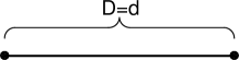
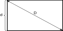
Figure 1: Illustration of diameters $d$ and $D$ in 1D (left) and 2D (right).

This gap conjecture was rigorously proved by Andrews and Clutterbuck [2]. The lower bound of the fundamental gaps depends only on the diameter of the domains and is independent of the external potential $V(\mathbf{x})$ and the different shapes of $\Omega$. It is noted that the gap conjecture links the algebraic property (i.e. difference of the first two eigenvalues of the Schrödinger operator) with the geometric property of the bounded domain $\Omega$ (i.e. its diameter). Extension of the gap conjecture to the Schrödinger operator in the whole space with a harmonic-type potential, i.e. (1.1) with $\alpha=2$, was also given in [2]. Recently, we generalized the gap conjecture to the Gross-Pitaevskii equation (GPE) (or the nonlinear Schrödinger equation with cubic repulsive interaction) [11].

The definition (1.2) (or (1.3)) is usually called as the (classical) fractional Laplacian (see, for instance, [15, 16, 17, 36, 41] and references therein). In the literatures [12, 14, 19, 46] and references therein, there is another way – local fractional Laplacian denoted as $A^{(\alpha/2)}$ – to define the fractional Laplacian via the spectral decomposition of Laplacian [12, 14, 46]. To be more specific, for a bounded domain $\Omega\subset\mathbb{R}^{n}$, let $\lambda_{\mathbf{m}}$ and $u_{\mathbf{m}}$ ($\mathbf{m}\in\mathbb{N}^{d}$) be the eigenvalues and corresponding eigenfunctions of the Laplacian operator $-\Delta$ on $\Omega$ with the homogeneous Dirichlet boundary condition, i.e. (1.10) with $V_{{}_{\Omega}}(\mathbf{x})\equiv 0$. Then for any $\alpha\in(0,2)$ and $\phi(\mathbf{x})\in H_{0}^{1}(\Omega)$ with

(1.13) $$\phi(\mathbf{x})=\sum_{\mathbf{m}\in\mathbb{N}^{d}}a_{\mathbf{m}}\,u_{\mathbf{m}}(\mathbf{x}),\qquad\mathbf{x}\in\overline{\Omega},$$

we define the operator $A^{(\alpha/2)}$ in the following way

(1.14) $$A^{(\alpha/2)}\phi(\mathbf{x})=\sum_{\mathbf{m}\in\mathbb{N}^{d}}a_{\mathbf{m}}\,\lambda_{\mathbf{m}}^{\alpha/2}\,u_{\mathbf{m}}(\mathbf{x}),\qquad\mathbf{x}\in\overline{\Omega}.$$

Comparison between the local fractional Laplacian operator $A^{(\alpha/2)}$ via (1.14) and the classical fractional Laplacian operator $(-\Delta)^{\frac{\alpha}{2}}$ via (1.2) (or (1.3)) with zero extension on $\Omega^{c}$ can be found in [41]. When $\alpha=2$, both definitions are the same. However, when $0<\alpha<2$, they are quite different. One main difference is that the eigenfunctions of $A^{(\alpha/2)}$ is smooth inside $\Omega$ while the eigenfunctions of $(-\Delta)^{\frac{\alpha}{2}}$ is $C^{0,s}$ for some $s\in(0,1)$. And this Hölder regularity is optimal [41]. Then on the bounded domain $\Omega$, for $\phi\in H_{0}^{1}(\Omega)$, one can define the local fractional Schrödinger operator (local FSO) via the local fractional Laplacian as

(1.15) $$L_{\rm loc}\,\phi(\mathbf{x}):=\left[A^{(\alpha/2)}+V_{{}_{\Omega}}(\mathbf{x})\right]\phi(\mathbf{x}),\qquad\mathbf{x}\in\Omega.$$

Similarly, the fundamental gap of the local FSO (1.15) is denoted as

(1.16) $$\delta_{\rm loc}(\alpha):=\lambda_{2}(\alpha)-\lambda_{1}(\alpha)>0,\qquad 0<\alpha\leq 2.$$

where $0<\lambda_{1}(\alpha)<\lambda_{2}(\alpha)$ are the first two smallest eigenvales of the local FSO (1.15).

Due to the nonlocal property of the FSO, it is very challenging to study mathematically and numerically the eigenvalue problem (1.5) [26]. In one dimension (1D), some estimates and asymptotic approximations of eigenvalues of the FSO without potential (i.e. $V(\mathbf{x})\equiv 0$) have been derived (see [6, 20, 22, 31] and references therein). It is noteworthy that Duo and Zhang [23] introduced a finite difference scheme to solve the eigenvalue problems related to FSO in 1D. Nevertheless, to the best of our knowledge, not much is available about the numerical method for (1.5) in multi-dimensions. The main purpose of this paper is to study asymptotically and numerically the fundamental gap $\delta(\alpha)$ of the FSO (1.5) on bounded domains $\Omega$, i.e. the potential $V(\mathbf{x})=+\infty$ for $\mathbf{x}\in\Omega^{c}$, and $\delta_{\rm loc}(\alpha)$ of the local FSO (1.15). Based on our asymptotic results and extensive numerical results, we propose the following:

Gap Conjecture I (Fundamental gaps of FSO on bounded domain with homogeneous Dirichlet boundary conditions) Suppose $\Omega$ is a bounded convex domain and $V_{\Omega}(\mathbf{x})$ is convex and non-negative.

(i) For the fundamental gap of the local FSO (1.15), we have

(1.19) $$\delta_{\rm loc}(\alpha) \geq\left\{\begin{array}[]{ll}\frac{(2^{\alpha}-1)\pi^{\alpha}}{D^{\alpha}},&n=1,\\ \frac{\alpha\pi^{\alpha}}{(n+2)^{1-\alpha/2}}\frac{d^{2-\alpha}}{D^{2}},&n\geq 2,\\ \end{array}\right.\qquad 0<\alpha\leq 2.$$

(ii) For the fundamental gap of the (classical) FSO (1.1), we have

(1.20) $$\delta(\alpha)\geq\frac{\alpha\pi^{\alpha}}{(n+2)^{1-\alpha/2}}\frac{d^{2-\alpha}}{D^{2}},\qquad 0<\alpha\leq 2.$$

In addition, we also propose a gap conjecture for the FSO (1.1) in the whole space.

The paper is organised as follows. In Section 2, we study asymptotically and numerically the fundamental gaps of the local FSO (1.15) and formulate the gap conjecture (1.19). Similar results for the (classical) FSO (1.1) on bounded domains with homogeneous Dirichlet boundary conditions are presented in Section 3. In Section 4, we study asymptotically and numerically the fundamental gaps of the FSO (1.1) in the whole space and formulate a gap conjecture. Again, similar results for the FSO (1.1) on bounded domains with periodic boundary conditions are presented in Section 5. Finally, some conclusions are drawn in Section 6.

2 The fundamental gaps of the local FSO (1.15)

Consider the eigenvalue problem generated by the local FSO (1.15)

(2.1) $$\begin{split}&L_{\rm loc}\,\phi(\mathbf{x}):=\left[A^{(\alpha/2)}+V_{{}_{\Omega}}(\mathbf{x})\right]\phi(\mathbf{x})=\lambda\,\phi(\mathbf{x}),\qquad\mathbf{x}\in\Omega,\\ &\phi(\mathbf{x})=0,\qquad\mathbf{x}\in\Gamma:=\partial\Omega.\end{split}$$

We will investigate asymptotically and numerically the first two smallest eigenvalues and their corresponding eigenfunctions of (2.1) and then formulate the gap conjecture (1.19).

2.1 Scaling property

Introduce

(2.2) $$\tilde{\mathbf{x}}=\frac{\mathbf{x}}{D},\ \tilde{\Omega}=\{\tilde{\mathbf{x}}\ |\ \mathbf{x}=D\,\tilde{\mathbf{x}}\in\Omega\},\ \tilde{V}_{{}_{\tilde{\Omega}}}(\tilde{\mathbf{x}})=D^{\alpha}V_{{}_{\Omega}}(\mathbf{x})=D^{\alpha}V_{{}_{\Omega}}(D\tilde{\mathbf{x}}),\ \mathbf{x}\in\Omega,$$

and consider the re-scaled eigenvalue problem

(2.3) $$\begin{split}&\tilde{L}_{\rm loc}\,\tilde{\phi}(\tilde{\mathbf{x}}):=\left[\tilde{A}^{(\alpha/2)}+\tilde{V}_{{}_{\tilde{\Omega}}}(\tilde{\mathbf{x}})\right]\tilde{\phi}(\tilde{\mathbf{x}})=\tilde{\lambda}\,\tilde{\phi}(\tilde{\mathbf{x}}),\qquad\tilde{\mathbf{x}}\in\tilde{\Omega},\\ &\tilde{\phi}(\tilde{\mathbf{x}})=0,\qquad\tilde{\mathbf{x}}\in\tilde{\Gamma}:=\partial\tilde{\Omega},\end{split}$$

where $\tilde{A}^{(\alpha/2)}$ is defined as (1.14) with $\Omega$ replaced by $\tilde{\Omega}$, then we have

Lemma 1.

Let $\lambda$ be an eigenvalue of (2.1) and $\phi:=\phi(\mathbf{x})$ is the corresponding eigenfunction, then $\tilde{\lambda}=D^{\alpha}\lambda$ is an eigenvalue of (2.3) and $\tilde{\phi}:=\tilde{\phi}(\tilde{\mathbf{x}})=\phi(D\tilde{\mathbf{x}})=\phi(\mathbf{x})$ is the corresponding eigenfunction, which immediately imply the scaling property on the fundamental gap $\delta_{\rm loc}(\alpha)$ of (2.1) as

(2.4) $$\delta_{\rm loc}(\alpha)=\frac{\tilde{\delta}_{\rm loc}(\alpha)}{D^{\alpha}},\qquad 0<\alpha\leq 2,$$

where $\tilde{\delta}_{\rm loc}(\alpha)$ is the fundamental gap of (2.3) with the diameter of $\tilde{\Omega}$ as $1$.

Proof.

Assume $\lambda_{\mathbf{m}}$ be an eigenvalue of (1.10) with $V_{\Omega}(\mathbf{x})\equiv 0$ and $u_{\mathbf{m}}(\mathbf{x})$ be the corresponding eigenfunction, i.e. $u_{\mathbf{m}}(\mathbf{x})\in H_{0}^{1}(\Omega)$ satisfies

(2.5) $$-\Delta u_{\mathbf{m}}(\mathbf{x})=\lambda_{\mathbf{m}}u_{\mathbf{m}}(\mathbf{x}),\quad\mathbf{x}\in\Omega.$$

It is easy to see that

(2.6) $$-\Delta\tilde{u}_{\mathbf{m}}(\tilde{\mathbf{x}})=D^{2}\lambda_{\mathbf{m}}\tilde{u}_{\mathbf{m}}(\tilde{\mathbf{x}})=\tilde{\lambda}_{\mathbf{m}}\tilde{u}_{\mathbf{m}}(\tilde{\mathbf{x}}),\quad\tilde{\mathbf{x}}\in\tilde{\Omega},$$

where $\tilde{\lambda}_{\mathbf{m}}=D^{2}\lambda_{\mathbf{m}}$. Then for any $\tilde{\phi}(\tilde{\mathbf{x}})\in H_{0}^{1}(\tilde{\Omega})$, recalling the definition of the local fractional Laplacian (1.14), we get

(2.7) $$A^{(\alpha/2)}\phi(\mathbf{x}) = \sum_{\mathbf{m}\in\mathbb{N}^{d}}a_{\mathbf{m}}\,\lambda_{\mathbf{m}}^{\alpha/2}\,u_{\mathbf{m}}(\mathbf{x})=D^{-\alpha}\sum_{\mathbf{m}\in\mathbb{N}^{d}}a_{\mathbf{m}}\,(D^{2}\lambda_{\mathbf{m}})^{\alpha/2}\,u_{\mathbf{m}}(\mathbf{x})$$

$$= D^{-\alpha}\sum_{\mathbf{m}\in\mathbb{N}^{d}}a_{\mathbf{m}}\,(\tilde{\lambda}_{\mathbf{m}})^{\alpha/2}\,\tilde{u}_{\mathbf{m}}(\tilde{\mathbf{x}})=D^{-\alpha}\tilde{A}^{(\alpha/2)}\tilde{\phi}(\tilde{\mathbf{x}}),\qquad\mathbf{x}\in\Omega.$$

Plugging (2.7) into (2.1), noticing (2.3), we get

(2.8) $$\lambda\,\tilde{\phi}(\tilde{\mathbf{x}}) = \lambda\,\phi(\mathbf{x})=\left[A^{(\alpha/2)}+V_{{}_{\Omega}}(\mathbf{x})\right]\phi(\mathbf{x})=\left[D^{-\alpha}\tilde{A}^{(\alpha/2)}+V_{{}_{\Omega}}(D\tilde{\mathbf{x}})\right]\tilde{\phi}(\tilde{\mathbf{x}})$$

$$= D^{-\alpha}\left[\tilde{A}^{(\alpha/2)}+D^{\alpha}V_{{}_{\Omega}}(D\tilde{\mathbf{x}})\right]\tilde{\phi}(\tilde{\mathbf{x}})=D^{-\alpha}\left[\tilde{A}^{(\alpha/2)}+\tilde{V}_{{}_{\tilde{\Omega}}}(\tilde{\mathbf{x}})\right]\tilde{\phi}(\tilde{\mathbf{x}}),$$

where $\mathbf{x}\in\Omega$ and $\tilde{\mathbf{x}}\in\tilde{\Omega}$, which immediately implies that $\tilde{\phi}(\tilde{\mathbf{x}})$ is an eigenfunction of the operator $\tilde{A}^{(\alpha/2)}+\tilde{V}_{{}_{\tilde{\Omega}}}(\tilde{\mathbf{x}})$ with the eigenvalue $\tilde{\lambda}=D^{\alpha}\lambda$. ∎

From this scaling property, in our asymptotic analysis and numerical simulation, we need only consider $\Omega$ whose diameter is $1$ in (2.1).

2.2 Asymptotic results for simple geometry

Take $\Omega=\prod_{j=1}^{n}(0,L_{j})$ and $V_{{}_{\Omega}}(\mathbf{x})\equiv 0$ in (2.1). Without loss of generality, we assume $L_{1}\geq L_{2}\geq\ldots\geq L_{n}>0$. In this case, the first two smallest eigenvalues and their corresponding eigenfunctions of $-\Delta$ can be chosen explicitly as [8, 10]

(2.9) $$\begin{split}&\lambda_{1}=\sum_{j=1}^{n}\frac{\pi^{2}}{L_{j}^{2}},\qquad\phi_{1}(\mathbf{x})=2^{n/2}\prod_{j=1}^{n}\sin\left(\frac{\pi x_{j}}{L_{j}}\right),\qquad\mathbf{x}\in\overline{\Omega},\\ &\lambda_{2}=\frac{4\pi^{2}}{L_{1}^{2}}+\sum_{j=2}^{n}\frac{\pi^{2}}{L_{j}^{2}},\qquad\phi_{2}(\mathbf{x})=2^{n/2}\sin\left(\frac{2\pi x_{j}}{L_{1}}\right)\prod_{j=2}^{n}\sin\left(\frac{\pi x_{j}}{L_{j}}\right).\\ \end{split}$$

By using the definition of the local FSO, we can obtain the first two smallest eigenvalues and the fundamental gap in this case as

(2.10) $$\begin{split}&\lambda_{1}(\alpha)=\left(\sum_{j=1}^{n}\frac{\pi^{2}}{L_{j}^{2}}\right)^{\alpha/2},\qquad\lambda_{2}(\alpha)=\left(\frac{4\pi^{2}}{L_{1}^{2}}+\sum_{j=2}^{n}\frac{\pi^{2}}{L_{j}^{2}}\right)^{\alpha/2},\\ &\delta_{\rm loc}(\alpha)=\lambda_{2}(\alpha)-\lambda_{1}(\alpha),\qquad 0<\alpha\leq 2.\end{split}$$

Formally, when $n\geq 2$, let $L_{2},\dots,L_{n}\to 0^{+}$ in (2.10), we have the diameter $D\to L_{1}$ and $\nu:=\left(\sum_{j=2}^{n}\frac{\pi^{2}}{L_{j}^{2}}\right)^{1/2}\to+\infty$. When $\alpha=2$,

(2.11) $$\delta_{\rm loc}(2)=\frac{3\pi^{2}}{L_{1}^{2}}=\frac{3\pi^{2}}{D^{2}}>0,$$

i.e. the fundamental gap is independent of the shape of the geometry and it only depends the diameter $D$ of $\Omega$. On the contrary, when $0<\alpha<2$,

(2.12) $$\delta_{\rm loc}(\alpha) = \left(\nu^{2}+\frac{4\pi^{2}}{L_{1}^{2}}\right)^{\alpha/2}-\left(\nu^{2}+\frac{\pi^{2}}{L_{1}^{2}}\right)^{\alpha/2}$$

$$= \nu^{\alpha}\left[\left(1+\frac{4\pi^{2}}{\nu^{2}L_{1}^{2}}\right)^{\alpha/2}-\left(1+\frac{\pi^{2}}{\nu^{2}L_{1}^{2}}\right)^{\alpha/2}\right]$$

$$= \frac{\alpha\nu^{\alpha}}{2}\;\frac{1}{(1+\xi)^{1-\alpha/2}}\;\frac{3\pi^{2}}{\nu^{2}L_{1}^{2}}$$

$$\leq \frac{3\alpha\pi^{2}}{L_{1}^{2}\,\nu^{2-\alpha}}\to 0^{+},\qquad 0<\alpha<2,$$

where $0<\xi\in[\pi^{2}/(\nu^{2}L_{1}^{2}),3\pi^{2}/(\nu^{2}L_{1}^{2})]$. In this case, the lower bound of the fundamental gap depends not only on the diameter $D$ of $\Omega$ but also another geometry quantity. By looking carefully at (2.12), we find that the diameter of the largest inscribed ball of $\Omega$, i.e. $d$, seems to be a good choice since its ratio with the diameter $D$ can be used to measure whether the domain degenerates from $n$ dimensions to lower dimensions. Based on these observation, we have the following lemma.

Lemma 2.

For $\Omega=\prod_{j=1}^{n}(0,L_{j})$ satisfying $L_{1}\geq L_{2}\geq\ldots\geq L_{n}>0$ and $V_{{}_{\Omega}}(\mathbf{x})\equiv 0$ in (2.1), we have the following lower bound of the fundamental gaps of the local FSO in (2.1)

(2.13) $$\delta_{\rm loc}(\alpha)\geq\left\{\begin{array}[]{ll}\frac{(2^{\alpha}-1)\pi^{\alpha}}{D^{\alpha}},&n=1,\\ \frac{\alpha\pi^{\alpha}}{(n+2)^{1-\alpha/2}}\frac{d^{2-\alpha}}{D^{2}},&n\geq 2,\\ \end{array}\right.\qquad 0<\alpha\leq 2,$$

where $D=\sqrt{\sum_{j=1}^{n}L_{j}^{2}}$ is the diameter of $\Omega$ and $d=L_{n}$ is the diameter of the largest inscribed ball in $\Omega$.

Proof.

When $n=1$, noticing $D=L_{1}$ and (2.10) with $n=1$, we have

(2.14) $$\delta_{\rm loc}(\alpha) = \lambda_{2}(\alpha)-\lambda_{1}(\alpha)=\left(\frac{4\pi^{2}}{L_{1}^{2}}\right)^{\alpha/2}-\left(\frac{\pi^{2}}{L_{1}^{2}}\right)^{\alpha/2}$$

$$= \frac{(2^{\alpha}-1)\pi^{\alpha}}{L_{1}^{\alpha}}=\frac{(2^{\alpha}-1)\pi^{\alpha}}{D^{\alpha}},\qquad 0<\alpha\leq 2.$$

Thus (2.13) is proved when $n=1$.

When $n\geq 2$, noticing (2.10), we have

(2.15) $$\delta_{\rm loc}(\alpha)=\left(\frac{4\pi^{2}}{L_{1}^{2}}+\sum_{j=2}^{n}\frac{\pi^{2}}{L_{j}^{2}}\right)^{\alpha/2}-\left(\frac{\pi^{2}}{L_{1}^{2}}+\sum_{j=2}^{n}\frac{\pi^{2}}{L_{j}^{2}}\right)^{\alpha/2},\qquad 0<\alpha\leq 2.$$

We will first prove that

(2.16) $$\delta_{\rm loc}(\alpha)\geq\left(\frac{4\pi^{2}}{D^{2}}+\frac{(n-1)\pi^{2}}{d^{2}}\right)^{\alpha/2}-\left(\frac{\pi^{2}}{D^{2}}+\frac{(n-1)\pi^{2}}{d^{2}}\right)^{\alpha/2},\qquad 0<\alpha\leq 2.$$

In order to do so, we consider two functions

(2.17) $$\begin{split}&f(x;C)=\left(\frac{4\pi^{2}}{x^{2}}+C^{2}\right)^{\alpha/2}-\left(\frac{\pi^{2}}{x^{2}}+C^{2}\right)^{\alpha/2},\qquad x>0,\\ &g(x;A,B)=\left(x+A+B\right)^{\alpha/2}-\left(x+A\right)^{\alpha/2},\\ \end{split}$$

where $0<\alpha\leq 2$, $C\in\mathbb{R}$ and $A,B\geq 0$. A direct computation shows that $\frac{d}{dx}f(x;C)\leq 0$ and $\frac{d}{dx}g(x;A,B)\leq 0$ for $x>0$, which means that $f(x;C)$ and $g(x;A,B)$ are monotonically decreasing functions. When $n=2$, it is easy to check that $d=L_{2}$ and $D\geq L_{1}$. Noticing $f(D;\pi/d)\leq f(L_{1};\pi/d)$, we immediately obtain (2.16) when $n=2$. When $n=3$, noting $d=L_{3}\leq L_{2}\leq L_{1}$ and $D\geq L_{1}\geq L_{2}\geq L_{3}$, we get

(2.18) $$\delta_{\rm loc}(\alpha) = \left(\frac{\pi^{2}}{L_{2}^{2}}+\frac{\pi^{2}}{L_{1}^{2}}+\frac{\pi^{2}}{L_{3}^{2}}+\frac{3\pi^{2}}{L_{1}^{2}}\right)^{\alpha/2}-\left(\frac{\pi^{2}}{L_{2}^{2}}+\frac{\pi^{2}}{L_{1}^{2}}+\frac{\pi^{2}}{L_{3}^{2}}\right)^{\alpha/2}$$

$$= g\left(\frac{\pi^{2}}{L_{2}^{2}};\frac{\pi^{2}}{L_{1}^{2}}+\frac{\pi^{2}}{L_{3}^{2}},\frac{3\pi^{2}}{L_{1}^{2}}\right)\geq g\left(\frac{\pi^{2}}{d^{2}};\frac{\pi^{2}}{L_{1}^{2}}+\frac{\pi^{2}}{L_{3}^{2}},\frac{3\pi^{2}}{L_{1}^{2}}\right)$$

$$= \left(\frac{4\pi^{2}}{L_{1}^{2}}+\frac{2\pi^{2}}{d^{2}}\right)^{\alpha/2}-\left(\frac{\pi^{2}}{L_{1}^{2}}+\frac{2\pi^{2}}{d^{2}}\right)^{\alpha/2}=f\left(L_{1};\frac{\sqrt{2}\pi}{d}\right)\geq f\left(D;\frac{\sqrt{2}\pi}{d}\right)$$

$$= \left(\frac{4\pi^{2}}{D^{2}}+\frac{2\pi^{2}}{d^{2}}\right)^{\alpha/2}-\left(\frac{\pi^{2}}{D^{2}}+\frac{2\pi^{2}}{d^{2}}\right)^{\alpha/2},\qquad 0<\alpha\leq 2,$$

which proves (2.16) when $n=3$.

When $n\geq 2$, noting (2.16), we get

(2.19) $$\delta_{\rm loc}(\alpha) \geq \left(\frac{4\pi^{2}}{D^{2}}+\frac{(n-1)\pi^{2}}{d^{2}}\right)^{\alpha/2}-\left(\frac{\pi^{2}}{D^{2}}+\frac{(n-1)\pi^{2}}{d^{2}}\right)^{\alpha/2}$$

$$= \left(\frac{(n-1)\pi^{2}}{d^{2}}\right)^{\alpha/2}\left[\left(1+\frac{3}{n-1}\left(\frac{d}{D}\right)^{2}\right)^{\alpha/2}-\left(1+\frac{1}{n-1}\left(\frac{d}{D}\right)^{2}\right)^{\alpha/2}\right]$$

$$= \left(\frac{(n-1)\pi^{2}}{d^{2}}\right)^{\alpha/2}\;\frac{\alpha}{n-1}\;\frac{1}{(1+\xi)^{1-\alpha/2}}\;\left(\frac{d}{D}\right)^{2},\qquad 0<\alpha\leq 2,$$

where the last equation is due to the mean value theorem with $\xi\in[\frac{1}{n-1}\left(\frac{d}{D}\right)^{2},\frac{3}{n-1}\left(\frac{d}{D}\right)^{2}]\subset[0,\frac{3}{n-1}]$. Noting that $\frac{1}{(1+\xi)^{1-\alpha/2}}$ is a decreasing function when $\xi\geq 0$ and taking $\xi=\frac{3}{n-1}$ in (2.19), we obtain the result (2.10) when $n\geq 2$ by (2.16) and (2.19). ∎

Remark 2.1.

When $n=1$, noting $d=D=L_{1}$, we have

(2.20) $$\delta_{\rm loc}(\alpha)\geq\frac{(2^{\alpha}-1)\pi^{\alpha}}{D^{\alpha}}\geq\frac{\alpha\pi^{\alpha}}{3^{1-\alpha/2}}\frac{d^{2-\alpha}}{D^{2}},\qquad 0<\alpha\leq 2.$$

Combing (2.20) and (2.13) with $n\geq 2$, we have a unified local bound of the fundamental gap of the local FSO as

(2.21) $$\delta_{\rm loc}(\alpha)\geq\frac{\alpha\pi^{\alpha}}{(n+2)^{1-\alpha/2}}\frac{d^{2-\alpha}}{D^{2}},\qquad 0<\alpha\leq 2,\quad 1\leq n\leq 3.$$

Of course, the lower bound is not sharp when $n=1$.

2.3 Numerical results for complicated geometry and/or general potentials

When $\Omega$ is a complicated domain and/or $V_{{}_{\Omega}}(\mathbf{x})\neq 0$ in (2.1), it is not generally possible to find the first two smallest eigenvalues explicitly. However, we can always compute numerically the first two smallest eigenvalues and their gap of (2.1) under a given bounded convex domain $\Omega$ and a convex real-valued function $V_{{}_{\Omega}}(\mathbf{x})$. Some numerical methods for local fractional Laplacian have been proposed in the literatures, e.g., a matrix representation of local fractional Laplacian operator based on a finite difference method is presented in [28, 29]; Fourier spectral methods for solving local fractional Laplacian can be found in e.g., [13, 1]. Recently, Sheng et al. [42] proposed a Fourierization of Legendre-Galerkin method for PDEs with local fractional Laplacian. The method retains the simplicity of Fourier method but is applicable to problems with non-periodic boundary conditions. In this paper, we adopt this method to numerically compute the first two smallest eigenvalues of (2.1).

Fig. 2 shows the numerical results on the fundamental gap $\delta_{\rm loc}(\alpha)$ of (2.1) when $n=1$, $\Omega=(0,1)$ and different external potentials $V_{{}_{\Omega}}(x)$. Fig. 3 shows similar results when $n=2$, $V_{{}_{\Omega}}(x,y)=(x^{2}+y^{2})/2$ and $\Omega=(0,d)\times(0,\sqrt{1-d^{2}})$ with different $0<d<1$; and $V_{{}_{\Omega}}(x,y)\equiv 0$ and $\Omega=\{(x,y)\ |\ x^{2}+y^{2}/d^{2}<1\}$ with different $0<d\leq 1$.

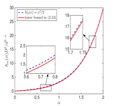
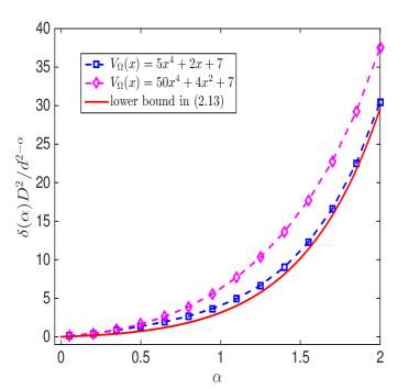
Figure 2: Comparison of the lower bound in (2.13) (solid line) and numerical results (dash lines) for the fundamental gap $\delta_{\rm loc}(\alpha)$ of the local FSO (2.1) with $n=1$, $\Omega=(0,1)$ and $V_{{}_{\Omega}}(x)=x^{2}/2$ (left) or other different convex potentials (right).

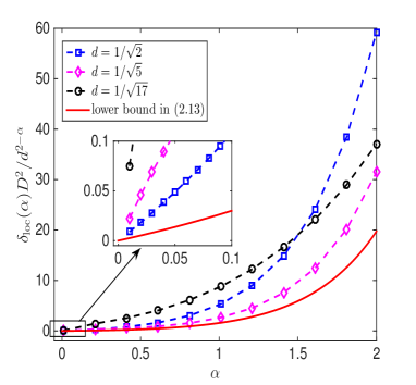
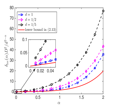
Figure 3: Comparison of the lower bound in (2.13) (solid line) and numerical results (dash lines) for the fundamental gap $\delta_{\rm loc}(\alpha)$ of the local FSO (2.1) with $n=2$, $V_{{}_{\Omega}}(x,y)=(x^{2}+y^{2})/2$ and $\Omega=(0,d)\times(0,\sqrt{1-d^{2}})$ under different $0<d<1$ (left); and $V_{{}_{\Omega}}(x,y)\equiv 0$ and $\Omega=\{(x,y)\ |\ x^{2}+y^{2}/d^{2}<1\}$ with different $0<d\leq 1$ (right).

Based on our asymptotic results in the previous subsection and numerical results in Figs. 2&3 as well as extensive more numerical results which draw similar conclusion and thus are not shown here for brevity, we are confident to formulate the gap conjecture (1.19) for the local FSO (1.15).

3 The fundamental gaps of the FSO (1.1) on bounded domains

Consider the eigenvalue problem generated by the FSO (1.1)

(3.1) $$\begin{split}&L_{\rm FSO}\,\phi(\mathbf{x}):=\left[(-\Delta)^{\frac{\alpha}{2}}+V_{{}_{\Omega}}(\mathbf{x})\right]\phi(\mathbf{x})=E\,\phi(\mathbf{x}),\qquad\mathbf{x}\in\Omega,\\ &\phi(\mathbf{x})=0,\qquad\mathbf{x}\in\Omega^{c}.\end{split}$$

In fact, if $\phi(\mathbf{x})$ is an eigenfunction normalized as

(3.2) $$\|\phi\|^{2}:=\int_{\mathbb{R}^{n}}\,|u(\mathbf{x})|^{2}\,d\mathbf{x}=\int_{\Omega}\,|u(\mathbf{x})|^{2}\,d\mathbf{x}=1,$$

then the corresponding eigenvalue $E>0$ can also be computed as

(3.3) $$E: = E^{(\alpha)}(\phi)=\int_{\Omega}\,\left[\phi(\mathbf{x})^{*}(-\Delta)^{\alpha/2}\phi(\mathbf{x})+V_{{}_{\Omega}}(\mathbf{x})|\phi(\mathbf{x})|^{2}\right]\,d\mathbf{x}$$

$$= \int_{{\mathbb{R}}^{n}}|\mathbf{k}|^{\alpha}|\hat{\phi}(\mathbf{k})|^{2}\,d\mathbf{k}+\int_{\Omega}\,V_{{}_{\Omega}}(\mathbf{x})|\phi(\mathbf{x})|^{2}\,d\mathbf{x},$$

where $\hat{\phi}:=\hat{\phi}(\mathbf{k})$ is the Fourier transform of $\phi:=\phi(\mathbf{x})$. We will investigate asymptotically and numerically the first two smallest eigenvalues and their corresponding eigenfunctions of (3.1) and then formulate the gap conjecture (1.20).

3.1 Scaling property

Under the transformation (2.2), consider the re-scaled eigenvalue problem

(3.4) $$\begin{split}&\tilde{L}_{\rm FSO}\,\tilde{\phi}(\tilde{\mathbf{x}}):=\left[(-\Delta)^{\frac{\alpha}{2}}+\tilde{V}_{{}_{\tilde{\Omega}}}(\tilde{\mathbf{x}})\right]\tilde{\phi}(\tilde{\mathbf{x}})=\tilde{E}\,\tilde{\phi}(\tilde{\mathbf{x}}),\qquad\tilde{\mathbf{x}}\in\tilde{\Omega},\\ &\tilde{\phi}(\tilde{\mathbf{x}})=0,\qquad\tilde{\mathbf{x}}\in\tilde{\Omega}^{c}.\end{split}$$

Then we have

Lemma 3.

Let $E$ be an eigenvalue of (3.1) and $\phi:=\phi(\mathbf{x})$ is the corresponding eigenfunction, then $\tilde{E}=D^{\alpha}E$ is an eigenvalue of (3.4) and $\tilde{\phi}:=\tilde{\phi}(\tilde{\mathbf{x}})=\phi(D\tilde{\mathbf{x}})=\phi(\mathbf{x})$ is the corresponding eigenfunction, which immediately imply the scaling property on the fundamental gap $\delta(\alpha)$ of (3.1) as

(3.5) $$\delta(\alpha)=\frac{\tilde{\delta}(\alpha)}{D^{\alpha}},\qquad 0<\alpha\leq 2,$$

where $\tilde{\delta}(\alpha)$ is the fundamental gap of (3.4) with the diameter of $\tilde{\Omega}$ as $1$.

Proof.

From (1.3), a direct computation implies the scaling property of the fractional Laplacian operator

(3.6) $$(-\Delta)^{\alpha/2}\phi(\mathbf{x}) = C_{n,\alpha}\int_{\mathbb{R}^{n}}\frac{\phi(\mathbf{x})-\phi(\mathbf{y})}{|\mathbf{x}-\mathbf{y}|^{n+\alpha}}\,d\mathbf{y}=C_{n,\alpha}\int_{\mathbb{R}^{n}}\frac{\phi(D\tilde{\mathbf{x}})-\phi(D\tilde{\mathbf{y}})}{|D\tilde{\mathbf{x}}-D\tilde{\mathbf{y}}|^{n+\alpha}}\,D^{n}\,{d\tilde{\mathbf{y}}}$$

$$= D^{-\alpha}C_{n,\alpha}\int_{\mathbb{R}^{n}}\frac{\tilde{\phi}(\tilde{\mathbf{x}})-\tilde{\phi}(\tilde{\mathbf{y}})}{|\tilde{\mathbf{x}}-\tilde{\mathbf{y}}|^{n+\alpha}}\,d\tilde{\mathbf{y}}=D^{-\alpha}\,(-\Delta)^{\alpha/2}\tilde{\phi}(\tilde{\mathbf{x}}),\quad\mathbf{x}\in\Omega,\ \tilde{\mathbf{x}}\in\tilde{\Omega}.$$

Noticing

(3.7) $$\phi(\mathbf{x})=0,\quad\mathbf{x}\in\Omega^{c}\qquad\Longleftrightarrow\qquad\tilde{\phi}(\tilde{\mathbf{x}})=0,\quad\tilde{\mathbf{x}}\in\tilde{\Omega}^{c}.$$

Substituting (3.6) into (3.1), noting (3.4), we get

(3.8) $$E\,\tilde{\phi}(\tilde{\mathbf{x}}) = E\,\phi(\mathbf{x})=\left[(-\Delta)^{\frac{\alpha}{2}}+V_{{}_{\Omega}}(\mathbf{x})\right]\phi(\mathbf{x})=\left[D^{-\alpha}\,(-\Delta)^{\frac{\alpha}{2}}+V_{{}_{\Omega}}(D\tilde{\mathbf{x}})\right]\tilde{\phi}(\tilde{\mathbf{x}})$$

$$= D^{-\alpha}\left[(-\Delta)^{\frac{\alpha}{2}}+D^{\alpha}V_{{}_{\Omega}}(D\tilde{\mathbf{x}})\right]\tilde{\phi}(\tilde{\mathbf{x}})=D^{-\alpha}\left[(-\Delta)^{\frac{\alpha}{2}}+\tilde{V}_{{}_{\tilde{\Omega}}}(\tilde{\mathbf{x}})\right]\tilde{\phi}(\tilde{\mathbf{x}}),$$

where $\mathbf{x}\in\Omega$ and $\tilde{\mathbf{x}}\in\tilde{\Omega}$, which immediately implies that $\tilde{\phi}(\tilde{\mathbf{x}})$ is an eigenfunction of the operator $(-\Delta)^{\frac{\alpha}{2}}+\tilde{V}_{{}_{\tilde{\Omega}}}(\tilde{\mathbf{x}})$ with the eigenvalue $\tilde{E}=D^{\alpha}E$. ∎

3.2 Asymptotic results when $0\leq 2-\alpha\ll 1$

For the fundamental gap $\delta(\alpha)$ of the FSO (1.1) in 1D with box potential, we have

Lemma 4.

Taken $n=1$, $\Omega=(0,1)$ and $V_{{}_{\Omega}}(x)\equiv 0$ for $x\in\Omega$ in (3.1), when $0\leq\varepsilon:=2-\alpha\ll 1$, we have

$$\delta(\alpha)\approx -\frac{2\pi^{2}}{\Gamma(4-\alpha)}\sec(\alpha\pi/2)\left[4\,\,_{1}F_{2}(2;2-\alpha/2,5/2-\alpha/2;-\pi^{2})\right.$$

(3.9) $$\left.+\,\,_{1}F_{2}(2;2-\alpha/2,5/2-\alpha/2;-\pi^{2}/4)\right],$$

where ${}_{p}F_{q}(a_{1},\dots,a_{p};b_{1},\dots,b_{q};z)$ is the generalized hypergeometric function defined as [5, 21]

(3.10) $$_{p}F_{q}(a_{1},\dots,a_{p};b_{1},\dots,b_{q};z)=\sum_{k=0}^{\infty}\frac{(a_{1})_{k}\dots(a_{p})_{k}}{(b_{1})_{k}\dots(b_{q})_{k}}\frac{z^{k}}{k!},$$

with $(a)_{0}=1$ and $(a)_{k}=a(a+1)\dots(a+k-1)$.

Proof.

For $n=1$, $\Omega=(0,1)$ and $V_{{}_{\Omega}}(x)\equiv 0$ in (3.1), when $\alpha=2$, the first two smallest eigenvalues and their corresponding normalized eigenfunctions can be given as [8, 10]

(3.11) $$E_{l}(2)=l^{2}\pi^{2},\qquad\phi_{l}(x)=\left\{\begin{array}[]{ll}\sqrt{2}\sin(l\pi x),&\text{ if }x\in(0,1)\\ 0,&\text{ otherwise,}\\ \end{array}\right.\quad l=1,2.$$

The Fourier transform of $\phi_{l}(x)$ ($l=1,2$) can be computed as

(3.12) $$\hat{\phi}_{l}(k)=\frac{\sqrt{2}l\pi((-1)^{l}e^{-ik}-1)}{k^{2}-l^{2}\pi^{2}},\qquad k\in{\mathbb{R}}.$$

It is worth noticing that $k=\pm l\pi$ are not singular points of $\hat{\phi}_{l}(k)$. In fact, we have that $\lim_{k\to l\pi}\hat{\phi}_{l}(k)=-i/2$ and $\lim_{k\to-l\pi}\hat{\phi}_{l}(k)=i/2$. When $\alpha$ satisfies $0\leq 2-\alpha\ll 1$, the two normalized eigenfunctions $\phi_{l}^{(\alpha)}(x)$ ($l=1,2$) corresponding to the first two smallest eigenvalues of (3.1) can be well approximated by $\phi_{l}(x)$ ($l=1,2$), respectively, i.e.

(3.13) $$\phi_{1}^{(\alpha)}(x)\approx\phi_{1}(x),\qquad\phi_{2}^{(\alpha)}(x)\approx\phi_{2}(x),\qquad x\in{\mathbb{R}}.$$

Substituting (3.13) into (3.3), noting (3.12), we can obtain the approximations of the first two smallest eigenvalues $E_{l}(\alpha)$ ($l=1,2$) as

(3.14) $$E_{l}(\alpha) = E^{(\alpha)}(\phi_{l}^{(\alpha)})\approx E^{(\alpha)}(\phi_{l})=\int_{0}^{1}\,\phi_{l}(x)\,(-\Delta)^{\alpha/2}\phi_{l}(x)\,dx$$

$$= \frac{1}{2\pi}\int_{\mathbb{R}}\,|k|^{\alpha}|\hat{\phi}_{l}(k)|^{2}\,dk=2l^{2}\pi\int_{\mathbb{R}}\frac{1-(-1)^{l}\cos(k)}{(k^{2}-l^{2}\pi^{2})^{2}}|k|^{\alpha}\,dk,\quad l=1,2.$$

Combining (3.10) and (3.14), we obtain

(3.15) $$\begin{split}&E_{1}(\alpha)\approx\frac{2^{\alpha-2}\pi^{\frac{5}{2}}\sec(\alpha\pi/2)}{\Gamma\left(2-\frac{\alpha}{2}\right)\Gamma\left(\frac{5-\alpha}{2}\right)}\,\,_{1}F_{2}(2;2-\alpha/2,5/2-\alpha/2;-\pi^{2}/4),\\ &E_{2}(\alpha)\approx\frac{2^{\alpha}\pi^{\frac{5}{2}}\sec(\alpha\pi/2)}{\Gamma\left(2-\frac{\alpha}{2}\right)\Gamma\left(\frac{5-\alpha}{2}\right)}\,\,_{1}F_{2}(2;2-\alpha/2,5/2-\alpha/2;-\pi^{2}).\end{split}$$

Plugging (3.15) into (1.9), we obtain (4) immediately and the proof is completed. ∎

Similarly, taken $n=2$, $\Omega=(0,1)\times(0,L)$ with $0<L\leq 1$ and $V_{{}_{\Omega}}(\mathbf{x})\equiv 0$ for $\mathbf{x}\in\Omega$ in (3.1), when $0<\varepsilon:=2-\alpha\ll 1$, we have

(3.16) $$\begin{split}&E_{1}(\alpha)\approx\frac{\pi^{2}}{L^{3}}\iint_{\mathbb{R}^{2}}\,(k_{1}^{2}+k_{2}^{2})^{\alpha/2}\;\frac{2+2\cos(k_{1})}{(k_{1}^{2}-\pi^{2})^{2}}\;\frac{2+2\cos(k_{2}L)}{(k_{2}^{2}-\pi^{2}/L^{2})^{2}}\,dk_{1}dk_{2},\\ &E_{2}(\alpha)\approx\frac{4\pi^{2}}{L^{3}}\iint_{\mathbb{R}^{2}}\,(k_{1}^{2}+k_{2}^{2})^{\alpha/2}\;\frac{2-2\cos(k_{1})}{(k_{1}^{2}-4\pi^{2})^{2}}\;\frac{2+2\cos(k_{2}L)}{(k_{2}^{2}-\pi^{2}/L^{2})^{2}}\,dk_{1}dk_{2},\\ &\delta(\alpha)=E_{2}(\alpha)-E_{1}(\alpha).\end{split}$$

Then one can obtain an asymptotic approximation of $\delta(\alpha)=E_{2}(\alpha)-E_{1}(\alpha)$ when $0<2-\alpha\ll 1$. Extension to (3.1) with $n=3$, $\Omega=(0,1)\times(0,L_{1})\times(0,L_{2})$ with $0<L_{2}\leq L_{1}\leq 1$ and $V(\mathbf{x})\equiv 0$ for $\mathbf{x}\in\Omega$ can be done in a similar way. The details are omitted here for brevity.

Unlike the case for the local FSO, for the FSO (3.1), it is difficult to get a concise lower bound of $\delta(\alpha)$ based on the asymptotic result (4) in 1D and (3.16) in 2D. Since our aim is not to get an optimal lower bound of $\delta(\alpha)$, one idea is to check whether the lower bound for the local FSO obtained in the previous section remains valid for the FSO. In order to do so, Fig 4 compares the fundamental gaps of (3.1) obtained numerically, the asymptotic approximations given in (4) for 1D, and the lower bounds of $\delta_{\rm loc}(\alpha)$ given in (2.13) (or (1.19)) and (2.21) for $n=1$ and $0\leq 2-\alpha\ll 1$.

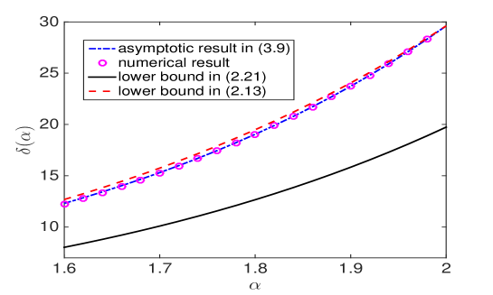
Figure 4: Comparison of the lower bound in (2.21) (solid line) and in (2.13) (dotted line), numerical results (dash line) and asymptotic results in (4) (dash-dot line) for the fundamental gap $\delta(\alpha)$ of the FSO (3.1) with $n=1$, $\Omega=(0,1)$ and $V_{{}_{\Omega}}(x)\equiv 0$ for $x\in\Omega$.

From Fig. 4, we can see that: (i) our asymptotic results agree with the numerical results very well when $0\leq 2-\alpha\ll 1$; (ii) the lower bound of $\delta_{\rm loc}(\alpha)$ given in (2.21) is still a lower bound of $\delta(\alpha)$; and (iii) when $n=1$, the lower bound of $\delta_{\rm loc}(\alpha)$ given in (1.19) is not a lower bound of $\delta(\alpha)$. With these observations, we will test numerically whether the lower bound of $\delta_{\rm loc}(\alpha)$ given in (2.21) is still a lower bound of $\delta(\alpha)$ for general geometry and general potential in the next subsection.

3.3 Numerical results for general potentials

Numerical solution of the eigenvalue problem (3.1) is very challenging due to the non-local boundary condition in an unbounded domain. There exist some numerical methods for PDEs with fractional Laplacian in unbounded domains based on finite-difference methods (cf. [23, 27] and spectral methods (cf. [30, 35]). In [43], we developed a promising method using the mapped Chebyshev functions for solving PDEs with fractional Laplacian in unbounded domain. We adopt this method to solve (3.1) numerically. Thanks to the scaling property shown in Lemma 3, the diameter of the domain $\Omega$ is always taken as $D=1$.

Fig. 5 shows the numerical results on the fundamental gap $\delta(\alpha)$ of (3.1) when $n=1$, $\Omega=(0,1)$ with different external potentials $V_{{}_{\Omega}}(x)$. Fig. 6 shows similar results with $n=2$, different $\Omega$ and different external potentials $V_{{}_{\Omega}}(x,y)$.

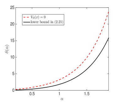
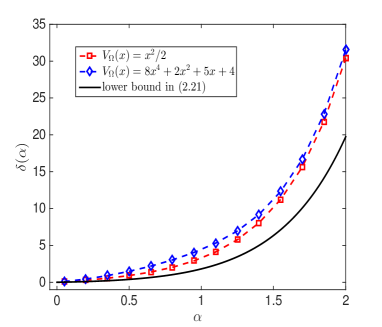
Figure 5: Comparison of the lower bound in (2.21) (solid line) and numerical results (dash lines) for the fundamental gap $\delta(\alpha)$ of the FSO (3.1) with $n=1$, $\Omega=(0,1)$ and $V_{{}_{\Omega}}(x)\equiv 0$ (left) or different convex potentials $V_{{}_{\Omega}}(x)$ (right).

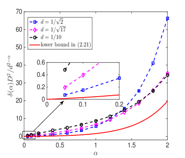
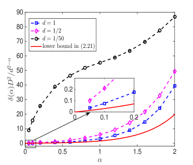
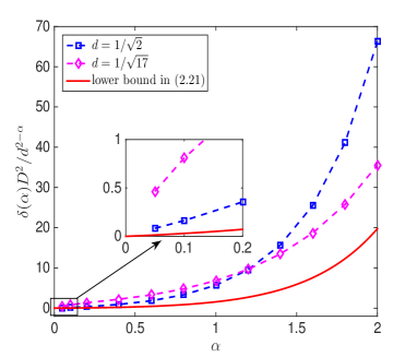
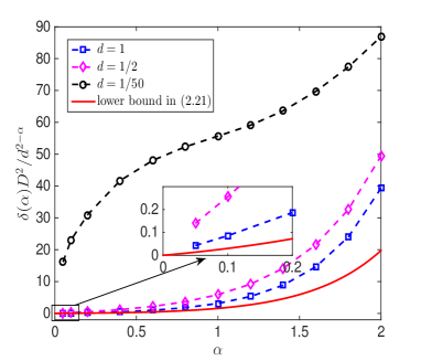
Figure 6: Comparison of the lower bound in (2.21) (solid line) and numerical results (dash lines) for the fundamental gap $\delta(\alpha)$ of the FSO (3.1) with $n=2$ and a rectangular type domain $\Omega=(0,d)\times(0,\sqrt{1-d^{2}})$ with different $0<d<1$(left); and an elliptic domain $\Omega=\{(x,y)\,|\,x^{2}+y^{2}/d^{2}\leq 1\}$ with different $0<d\leq 1$ (right). The external potential is chosen as $V_{{}_{\Omega}}(x,y)\equiv 0$ (top) or $V_{{}_{\Omega}}(x,y)=(x^{2}+y^{2})/2$ (bottom) in $\Omega$.

Again, based on our asymptotic results in the previous subsection and numerical results in Figs. 5&6 as well as extensive numerical results which draw similar conclusion and thus are not shown here for brevity, we are confident to formulate the gap conjecture (1.20) for the FSO (3.1).

4 The fundamental gaps of the FSO (1.1) in the whole space

In this section, we will study asymptotically and numerically the first two smallest eigenvalues and their corresponding eigenfunctions of the eigenvalue problem (1.5) generated by the FSO (1.1) in the whole space and then formulate a gap conjecture. Here we assume $V(\mathbf{x})\in L^{\infty}_{\rm loc}({\mathbb{R}}^{n})$.

In many applications [8], the following harmonic potential is widely used

(4.1) $$V(\mathbf{x})=\sum_{j=1}^{n}\gamma_{j}^{2}x_{j}^{2},\qquad\mathbf{x}=(x_{1},\ldots,x_{n})^{T}\in{\mathbb{R}}^{n},$$

where $\gamma_{1}>0$, $\ldots$, $\gamma_{n}>0$ are given positive constants. Without loss of generality, we assume that $0<\gamma_{1}\leq\ldots\leq\gamma_{n}$. Denote $\gamma:=\gamma_{1}$ and $\eta_{j}:=\frac{\gamma_{j}}{\gamma_{1}}\geq 1$ ($j=1,\ldots,n$) and $\eta=\max_{1\leq j\leq n}\eta_{j}=\eta_{n}=\frac{\gamma_{n}}{\gamma_{1}}\geq 1$, then the harmonic potential (4.2) can be re-written as

(4.2) $$V(\mathbf{x})=\gamma^{2}\sum_{j=1}^{n}\eta_{j}^{2}x_{j}^{2}=\gamma^{2}\left(x_{1}^{2}+\sum_{j=2}^{n}\eta_{j}^{2}x_{j}^{2}\right),\qquad\mathbf{x}=(x_{1},\ldots,x_{n})^{T}\in{\mathbb{R}}^{n}.$$

4.1 Scaling property

Introduce

(4.3) $$D:=\gamma^{-\frac{2}{2+\alpha}},\quad\tilde{\mathbf{x}}=\frac{\mathbf{x}}{D},\quad\tilde{V}(\tilde{\mathbf{x}})=\tilde{x}_{1}^{2}+\sum_{j=2}^{n}\eta_{j}^{2}\tilde{x}_{j}^{2},\quad\tilde{\phi}(\tilde{\mathbf{x}})=\phi(\mathbf{x}),\quad\mathbf{x},\tilde{\mathbf{x}}\in{\mathbb{R}}^{n},$$

and consider the re-scaled eigenvalue problem

(4.4) $$\tilde{L}_{\rm FSO}\,\tilde{\phi}(\tilde{\mathbf{x}}):=\left[(-\Delta)^{\frac{\alpha}{2}}+\tilde{V}(\tilde{\mathbf{x}})\right]\tilde{\phi}(\tilde{\mathbf{x}})=\tilde{E}\,\tilde{\phi}(\tilde{\mathbf{x}}),\qquad\tilde{\mathbf{x}}\in{\mathbb{R}}^{n},$$

then we have

Lemma 5.

Let $E$ be an eigenvalue of (1.5) with (4.2) and $\phi:=\phi(\mathbf{x})$ is the corresponding eigenfunction, then $\tilde{E}=\gamma^{-\frac{2\alpha}{2+\alpha}}E$ is an eigenvalue of (4.4) and $\tilde{\phi}:=\tilde{\phi}(\tilde{\mathbf{x}})=\phi(D\tilde{\mathbf{x}})=\phi(\mathbf{x})$ is the corresponding eigenfunction, which immediately imply the scaling property on the fundamental gap $\delta(\alpha)$ of (1.5) with (4.2) as

(4.5) $$\delta(\alpha)=\gamma^{\frac{2\alpha}{2+\alpha}}\;\tilde{\delta}(\alpha),\qquad 0<\alpha\leq 2,$$

where $\tilde{\delta}(\alpha)$ is the fundamental gap of (4.4).

Proof.

From (4.3), similar to (3.6), we have

(4.6) $$(-\Delta)^{\alpha/2}\phi(\mathbf{x})=D^{-\alpha}\,(-\Delta)^{\alpha/2}\tilde{\phi}(\tilde{\mathbf{x}}),\quad\mathbf{x},\tilde{\mathbf{x}}\in{\mathbb{R}}^{n}.$$

Substituting (4.6) into (1.5) with (4.2), noting (4.2)-(4.4), we get

(4.7) $$E\,\tilde{\phi}(\tilde{\mathbf{x}}) = E\,\phi(\mathbf{x})=\left[(-\Delta)^{\frac{\alpha}{2}}+V(\mathbf{x})\right]\phi(\mathbf{x})=\left[D^{-\alpha}\,(-\Delta)^{\frac{\alpha}{2}}+V(D\tilde{\mathbf{x}})\right]\tilde{\phi}(\tilde{\mathbf{x}})$$

$$= D^{-\alpha}\left[(-\Delta)^{\frac{\alpha}{2}}+D^{2+\alpha}\gamma^{2}\tilde{V}(\tilde{\mathbf{x}})\right]\tilde{\phi}(\tilde{\mathbf{x}})=\gamma^{\frac{2\alpha}{2+\alpha}}\left[(-\Delta)^{\frac{\alpha}{2}}+\tilde{V}(\tilde{\mathbf{x}})\right]\tilde{\phi}(\tilde{\mathbf{x}}),$$

where $\mathbf{x},\tilde{\mathbf{x}}\in{\mathbb{R}}^{n}$ and $D=\gamma^{-2/(2+\alpha)}$, which immediately implies that $\tilde{\phi}(\tilde{\mathbf{x}})$ is an eigenfunction of the operator $(-\Delta)^{\frac{\alpha}{2}}+\tilde{V}(\tilde{\mathbf{x}})$ with the eigenvalue $\tilde{E}=\gamma^{-\frac{2\alpha}{2+\alpha}}E$. ∎

4.2 Asymptotic results for harmonic potential when $0\leq 2-\alpha\ll 1$

Consider a harmonic potential in (1.5) as (4.1) (or (4.2)). By using the Fourier transform over ${\mathbb{R}}^{n}$, the eigenvalue problem (1.5) can be reformulated as a standard eigenvalue problem in the phase (or Fourier) space as, i.e. without the fractional Laplacian operator

(4.8) $$\left(-\sum_{j=1}^{n}\gamma_{j}^{2}\frac{\partial^{2}}{\partial k_{j}^{2}}+|\mathbf{k}|^{\alpha}\right)\hat{\phi}(\mathbf{k})=E\,\hat{\phi}(\mathbf{k}),\qquad\mathbf{k}=(k_{1},\ldots,k_{n})^{T}\in\mathbb{R}^{n},$$

where $\hat{\phi}(\mathbf{k})$ is the Fourier transform of $\phi(\mathbf{x})$ over the whole space $\mathbb{R}^{n}$. Introduce

(4.9) $$\tilde{k}_{j}=\frac{k_{j}}{\gamma_{j}},\quad j=1,\ldots,n,\quad\tilde{\phi}(\tilde{\mathbf{k}})=\phi(\mathbf{k})=\phi(\gamma_{1}\tilde{k}_{1},\ldots,\gamma_{n}\tilde{k}_{n}),\quad\mathbf{k},\tilde{\mathbf{k}}\in{\mathbb{R}}^{n},$$

then the eigenvalue problem (4.8) can be reformulated as an eigenvalue with the Laplacian

(4.10) $$\left(-\Delta+\left(\sum_{j=1}^{n}\gamma_{j}^{2}|\tilde{k}_{j}|^{2}\right)^{\alpha/2}\right)\tilde{\phi}(\tilde{\mathbf{k}})=E\,\tilde{\phi}(\tilde{\mathbf{k}}),\qquad\tilde{\mathbf{k}}=(\tilde{k}_{1},\ldots,\tilde{k}_{n})^{T}\in\mathbb{R}^{n},$$

In fact, if $\phi(\mathbf{x})\neq 0$ is an eigenfunction of (1.5) corresponding to the eigenvalue $E$, then $\hat{\phi}(\mathbf{k})\neq 0$ is an eigenfunction of (4.8) corresponding to the same eigenvalue $E$, and $\tilde{\phi}(\tilde{\mathbf{k}})\neq 0$ is an eigenfunction of (4.10) corresponding to the same eigenvalue $E$. In addition, we have

(4.11) $$E = \frac{1}{\int_{\mathbb{R}^{n}}|\hat{\phi}(\mathbf{k})|^{2}\,d\mathbf{k}}\int_{\mathbb{R}^{n}}\left(\sum_{j=1}^{n}\gamma_{j}^{2}\left|\frac{\partial\hat{\phi}(\mathbf{k})}{\partial k_{j}}\right|^{2}+|\mathbf{k}|^{\alpha}\left|\hat{\phi}(\mathbf{k})\right|^{2}\right)\,d\mathbf{k}$$

$$= \frac{1}{\int_{\mathbb{R}^{n}}|\tilde{\phi}(\tilde{\mathbf{k}})|^{2}\,d\tilde{\mathbf{k}}}\int_{\mathbb{R}^{n}}\left(|\nabla\tilde{\phi}(\tilde{\mathbf{k}})|^{2}+\left(\sum_{j=1}^{n}\gamma_{j}^{2}|\tilde{k}_{j}|^{2}\right)^{\alpha/2}\left|\tilde{\phi}(\tilde{\mathbf{k}})\right|^{2}\right)\,d\tilde{\mathbf{k}}.$$

Lemma 6.

Taken $n=1$ and a harmonic potential $V(x)$ as (4.2) in (1.5), when $0\leq\varepsilon:=2-\alpha\ll 1$, we have

(4.12) $$\delta(\alpha)\approx\gamma+\frac{\alpha\gamma^{\alpha/2}}{\sqrt{\pi}}\Gamma\left(\frac{1+\alpha}{2}\right).$$

Proof.

When $n=1$ and $\alpha=2$, the first two smallest eigenvalues and their corresponding eigenfunctions of the eigenvalue problem (1.5) with (4.2) can be given as [8, 10]

(4.13) $$\begin{split}&E_{1}(2)=\gamma,\qquad\phi_{1}(x)=\left(\frac{\gamma}{\pi}\right)^{1/4}e^{-\gamma x^{2}/2},\qquad x\in{\mathbb{R}},\\ &E_{2}(2)=3\gamma,\qquad\phi_{2}(x)=\sqrt{2\gamma}x\left(\frac{\gamma}{\pi}\right)^{1/4}e^{-\gamma x^{2}/2}.\\ \end{split}$$

The Fourier transform of $\phi_{l}(x)$ ($l=1,2$) can be computed as

(4.14) $$\hat{\phi}_{1}(k)=\frac{\sqrt{2}\pi^{1/4}}{\gamma^{1/4}}e^{-\frac{k^{2}}{2\gamma}},\quad\hat{\phi}_{2}(k)=\frac{-2i\pi^{1/4}}{\gamma^{3/4}}ke^{-\frac{k^{2}}{2\gamma}},\qquad k\in{\mathbb{R}}.$$

When $\alpha$ satisfies $0\leq 2-\alpha\ll 1$, the two normalized eigenfunctions $\phi_{l}^{(\alpha)}(x)$ ($l=1,2$) corresponding to the first two smallest eigenvalues of (1.5) can be well approximated by $\phi_{l}(x)$ ($l=1,2$), respectively, i.e.

(4.15) $$\phi_{1}^{(\alpha)}(x)\approx\phi_{1}(x),\qquad\phi_{2}^{(\alpha)}(x)\approx\phi_{2}(x),\qquad x\in{\mathbb{R}}.$$

Substituting (4.15) and (4.14) into (4.11), we can obtain the approximations of the first two smallest eigenvalues $E_{l}(\alpha)$ ($l=1,2$) as

(4.16) $$\begin{split}&E_{1}{(\alpha)}=E^{(\alpha)}(\phi_{1}^{(\alpha)})\approx E^{(\alpha)}(\phi_{1})=\frac{\gamma}{2}+\frac{\gamma^{\alpha/2}}{\sqrt{\pi}}\Gamma\left(\frac{1+\alpha}{2}\right),\\ &E_{2}{(\alpha)}=E^{(\alpha)}(\phi_{2}^{(\alpha)})\approx E^{(\alpha)}(\phi_{2})=\frac{3\gamma}{2}+\frac{2\gamma^{\alpha/2}}{\sqrt{\pi}}\Gamma\left(\frac{3+\alpha}{2}\right).\end{split}$$

Subtracting the first equation from the second equation in (4.16), we get

(4.17) $$\delta(\alpha) = E_{2}{(\alpha)}-E_{1}{(\alpha)}\approx\gamma+\frac{2\gamma^{\alpha/2}}{\sqrt{\pi}}\Gamma\left(1+\frac{1+\alpha}{2}\right)-\frac{\gamma^{\alpha/2}}{\sqrt{\pi}}\Gamma\left(\frac{1+\alpha}{2}\right)$$

$$= \gamma+\frac{(1+\alpha)\gamma^{\alpha/2}}{\sqrt{\pi}}\Gamma\left(\frac{1+\alpha}{2}\right)-\frac{\gamma^{\alpha/2}}{\sqrt{\pi}}\Gamma\left(\frac{1+\alpha}{2}\right)=\gamma+\frac{\alpha\gamma^{\alpha/2}}{\sqrt{\pi}}\Gamma\left(\frac{1+\alpha}{2}\right).$$

The proof is completed. ∎

Similarly, taken $n=2$ and $1=\gamma\leq\eta_{2}=\eta$ in (1.5) and (4.2), when $0\leq\varepsilon:=2-\alpha\ll 1$, we get (with details omitted here for brevity)

$$\delta(\alpha) \approx 1-\frac{1}{\pi\sqrt{\eta}}\iint\,(2k_{1}^{2}+1)(k_{1}^{2}+k_{2}^{2})^{\alpha}e^{-(k_{1}^{2}+k_{2}^{2}/\eta)}\,dk_{1}dk_{2}$$

$$=1-\frac{\Gamma(-(1+\alpha)/2)\Gamma(1+\alpha/2)}{\sqrt{\pi\eta}\Gamma(-\alpha/2)}\left[-_{2}F_{1}(1/2,1+\alpha/2;(3+\alpha)/2;1/\eta)\right.$$

$$\left.+(2+\alpha)\,\,\,_{2}F_{1}(1/2,2+\alpha/2;(3+\alpha)/2;1/\eta)\right]$$

$$+\frac{\alpha\sqrt{\pi}\eta^{\alpha/2}}{\eta-1}\left[-\eta\,\,\,_{2}F_{1}(-1/2,-\alpha/2;(1-\alpha)/2;1/\eta)/\Gamma((1-\alpha)/2)\right.$$

(4.18) $$\left.+(\eta-1)\,\,\,_{2}F_{1}(1/2,-\alpha/2;(1-\alpha)/2;1/\eta)/\Gamma((1-\alpha)/2)\sec(\alpha\pi)\right].$$

In order to verify the asymptotic results (4.12) in 1D and (4.18) in 2D when $0\leq 2-\alpha\ll 1$, Fig. 7 plots the asymptotic results and numerical results of the fundamental gap $\delta(\alpha)$ of the FSO (1.5) when $0\leq 2-\alpha\ll 1$. The results indicate that our asymptotic results are quite accurate in the regime $0\leq 2-\alpha\ll 1$ (cf. Fig. 7). In addition, we cannot get a lower bound of the fundamental gap $\delta(\alpha)$ from the asymptotic results!

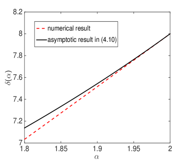
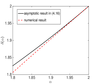
Figure 7: Comparison of the asymptotic results in (4.12) or (4.18) (solid line) and numerical results (dash lines) for the fundamental gap $\delta(\alpha)$ of the FSO (1.5) with $n=1$ and $V(x)=16x^{2}$ (left) and with $n=2$ and $V(x,y)=x^{2}+16y^{2}$ (right).

4.3 A formal lower bound on the fundamental gap in 2D

In order to get a lower bound of the fundamental gap $\delta(\alpha)$ of the FSO (1.5), we take $n=2$ and $V(x,y)=x^{2}+\eta^{2}y^{2}$ with $\eta\geq 1$ in (1.5) and consider the following eigenvalue problem

(4.19) $$\left[(-\Delta)^{\frac{\alpha}{2}}+(x^{2}+\eta^{2}y^{2})\right]\phi(\mathbf{x})=E\,\phi(\mathbf{x}),\qquad\mathbf{x}=(x,y)^{T}\in{\mathbb{R}}^{2}.$$

When $\alpha=2$, the first two smallest eigenvalues of (4.19) are [8, 10]

(4.20) $$E_{1}:=E_{1}(2)=1+\eta,\qquad E_{2}:=E_{2}(2)=3+\eta,\qquad\eta\geq 1.$$

Motivated by the methods and results in the previous two sections, we assume that the lower bound of the fundamental gap might depend on the parameter $\eta$ – the anisotropy of the harmonic potential. Similar to the case of the local FSO, i.e. finding the lower bound of the fundamental gap by estimating $\lambda_{2}^{\alpha/2}-\lambda_{1}^{\alpha/2}$ with $\lambda_{1}$ and $\lambda_{2}$ being the first two smallest eigenvalues of the corresponding operator when $\alpha=2$, we formally assume that the fundamental gap $\tilde{\delta}(\alpha)$ of (4.19) has a similar estimate as

(4.21) $$\tilde{\delta}(\alpha)\geq E_{2}^{\beta}-E_{1}^{\beta}=(3+\eta)^{\beta}-(1+\eta)^{\beta},$$

where $0<\beta\leq 1$ is to be determined in an asymptotic way by considering $\eta\to+\infty$. When $\eta\gg 1$, the eigenfunction of (4.19) varies extremely slow in the $x$-direction. As a result, the problem (4.19) can be formally well approximated by

(4.22) $$\left[(-\partial_{yy})^{\frac{\alpha}{2}}+\eta^{2}y^{2}\right]u(y)=E\,u(y),\qquad y\in{\mathbb{R}},$$

The scaling property in Lemma 5 implies that $E\sim\mathcal{O}(\eta^{2\alpha/(2+\alpha)})$, which indicates that one reasonable choice of $\beta$ is

(4.23) $$\beta=\frac{2\alpha}{2+\alpha}.$$

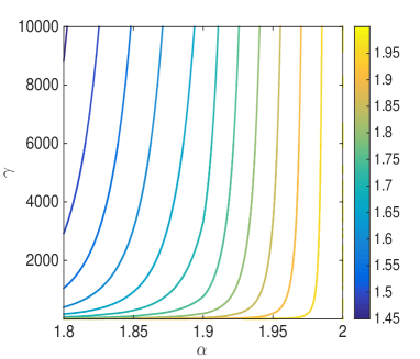
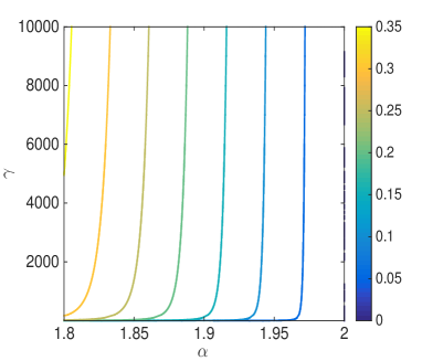
Figure 8: Comparison of the asymptotic results in (4.18) (left) and the lower bound in (4.25) (right) for the fundamental gap $\tilde{\delta}(\alpha)$ of the FSO (4.19) for different $\alpha$ and $\eta\geq 1$.

When $\eta\geq 1$, we have

$$\tilde{\delta}(\alpha)\geq\eta^{\beta}\left[\left(1+\frac{3}{\eta}\right)^{\beta}-\left(1+\frac{1}{\eta}\right)^{\beta}\right]=\eta^{\beta}\,\beta\,\frac{1}{(1+\xi)^{1-\beta}}\,\frac{2}{\eta}=\frac{2\beta\eta^{\beta-1}}{(1+\xi)^{1-\beta}},$$

where $\xi\in[1/\eta,3/\eta]\subset(0,3]$. Noting that $\frac{1}{(1+\xi)^{1-\beta}}$ is a decreasing function when $\xi\geq 0$ and taking $\xi=3$, we get

(4.24) $$\tilde{\delta}(\alpha)\geq 2\beta\eta^{\beta-1}\frac{1}{4^{1-\beta}}=\frac{4^{\beta}\beta}{2}\eta^{\beta-1}.$$

Plugging (4.23) into (4.24), we obtain a lower bound

(4.25) $$\tilde{\delta}(\alpha)\geq 2^{\frac{4\alpha}{2+\alpha}}\,\frac{\alpha}{2+\alpha}\;\frac{1}{\eta^{\frac{2-\alpha}{2+\alpha}}}.$$

To compare the asymptotic results (4.18) in 2D and the formal lower bound in (4.25) for the fundamental gap $\tilde{\delta}(\alpha)$ of the FSO (4.19), Fig. 8 shows the contour plot of (4.18) and the lower bound in (4.25) for different $\eta\geq 1$ and $\alpha$. It shows that (i) the asymptotic results in (4.18) degenerates to $0$ when either $\alpha\to 0^{+}$ or $\eta\to+\infty$ (cf. Fig. 8 (left)), and (ii) the lower bound in (4.25) does show the effect of the parameter $\eta\geq 1$ properly since the contour line is almost vertical when $\eta\gg 1$.

4.4 Numerical results for general potentials

Combining (4.25) and the scaling property in Lemma 5, noting (4.8) and (1.5) with (4.2), we can formally obtain a lower bound of the fundamental gap $\delta(\alpha)$ of the FSO (1.5) with (4.2)

(4.26) $$\delta(\alpha)=\gamma^{\frac{2\alpha}{2+\alpha}}\;\tilde{\delta}(\alpha)\geq 2^{\frac{4\alpha}{2+\alpha}}\,\frac{\alpha}{2+\alpha}\;\frac{\gamma^{\frac{2\alpha}{2+\alpha}}}{\eta^{\frac{2-\alpha}{2+\alpha}}}.$$

To verify numerically the lower bound in (4.26), Fig. 9 shows numerical results of the fundamental gap $\delta(\alpha)$ of (1.5) with (4.2).

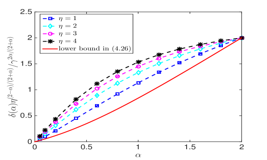
Figure 9: Comparison of the lower bound in (4.26) (solid line) and numerical results (dash lines) for the fundamental gap $\delta(\alpha)$ of the FSO (1.5) with $V(x,y)=\gamma^{2}(x^{2}+\eta^{2}y^{2})$ for different $\eta\geq 1$ and $\gamma>0$.

Furthermore, to check numerically whether the lower bound in (4.26) is still valid for (1.5) with general convex harmonic-type potentials, Fig. 10 shows numerical results of the fundamental gap $\delta(\alpha)$ of (1.5) with different potentials taken as Case I: $V(x,y)=2x^{2}+20y^{2}+\cos(x)+2\sin(2y)$ with $\gamma=\sqrt{6}/2$ and $\eta=4$; and Case II: $V(x,y)=x^{2}+100y^{2}+\cos(x)+10\sin(2y)$ with $\gamma=\sqrt{2}/2$ and $\eta=4\sqrt{15}$.

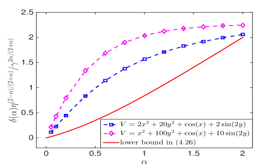
Figure 10: Comparison of the lower bound in (4.26) (solid line) and numerical results (dash lines) for the fundamental gap $\delta(\alpha)$ of the FSO (1.5) with different potentials $V(\mathbf{x})$.

Based on the asymptotic results and numerical results in this section, as well as extensive numerical results which draw similar conclusion and thus are not shown here for brevity, we can formulate the following:

Gap Conjecture II (For the FSO (1.5) in the whole space). Assume the potential $V(\mathbf{x})\in C^{2}({\mathbb{R}}^{n})$ in (1.5) satisfies

(4.27) $$\gamma_{1}^{2}I_{n}\leq\frac{1}{2}D^{2}V(\mathbf{x})\leq\gamma_{2}^{2}I_{n},\qquad\mathbf{x}\in{\mathbb{R}}^{n},$$

where $0<\gamma_{1}\leq\gamma_{2}$ are two positive constants and $I_{n}$ is the $n\times n$ identity matrix. Denote $\gamma=\gamma_{1}$ and set $\eta=\gamma_{2}/\gamma_{1}\geq 1$, then the fundamental gap $\delta(\alpha)$ of the FSO (1.5) can be bounded below by

(4.28) $$\delta(\alpha)\geq 2^{\frac{4\alpha}{2+\alpha}}\frac{\alpha}{2+\alpha}\frac{\gamma^{\frac{2\alpha}{2+\alpha}}}{\eta^{\frac{2-\alpha}{2+\alpha}}}=2^{\frac{4\alpha}{2+\alpha}}\frac{\alpha}{2+\alpha}\frac{\gamma_{1}}{\gamma_{2}^{\frac{2-\alpha}{2+\alpha}}},\qquad 0<\alpha\leq 2.$$

4.5 Numerical results for well potential

Consider a well potential in (1.5)

(4.29) $$V(\mathbf{x})=\begin{cases}0,&\text{for }\mathbf{x}\in\Omega,\\ V_{0},&\text{for }\mathbf{x}\in\Omega^{c},\end{cases}$$

for some $V_{0}>0$. We solve (1.5) with (4.29) numerically and compare the solutions with those in (3.1) and/or (2.1) by letting $V_{0}\to+\infty$. Denote $0<E_{1}^{V_{0}}<E_{2}^{V_{0}}<\ldots$ be the eigenvalues of (1.5) with (4.29) and $\phi_{1}^{V_{0}}(x)$, $\phi_{2}^{V_{0}}(x)$, $\ldots$ be the corresponding eigenfunctions. Similarly, denote $0<\lambda_{1}<\lambda_{2}<\ldots$ be the eigenvalues of (3.1) and $\phi_{1}(x)$, $\phi_{2}(x)$, $\ldots$ be the corresponding eigenfunctions; and denote $0<\tilde{\lambda}_{1}<\tilde{\lambda}_{2}<\ldots$ be the eigenvalues of (2.1) and $\tilde{\phi}_{1}(x)$, $\tilde{\phi}_{2}(x)$, $\ldots$ be the corresponding eigenfunctions. All the solutions are obtained numerically.

Fig. 11 shows $|E_{1}^{V_{0}}-\lambda_{1}|$ and $|E_{1}^{V_{0}}-\tilde{\lambda}_{1}|$ for different $0<\alpha\leq 2$ and $V_{0}>0$. Similarly, Fig. 12 shows $|\phi_{1}^{V_{0}}(x)-\phi_{1}(x)|$ and $|\phi_{1}^{V_{0}}(x)-\tilde{\phi}_{1}(x)|$ for $\alpha=1.5$ and different $V_{0}>0$. Numerical comparisons were also performed for other eigenvalues and their corresponding eigenfunctions, which draw similar conclusion and thus are not shown here for brevity.

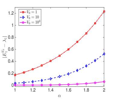
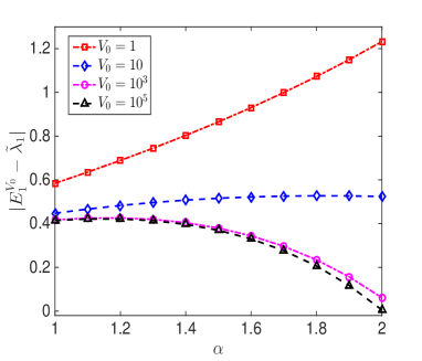
Figure 11: Comparison of eigenvalues of (1.5) with a box potential (4.29) and those of (3.1) and/or (2.1) for different $\alpha$ and $V_{0}$.

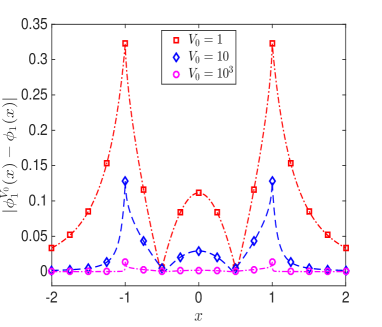
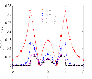
Figure 12: Comparison of eigenfunctions of (1.5) with a box potential (4.29) and those of (3.1) and/or (2.1) for $\alpha=1.5$ and different $V_{0}$.

From Figs. 11&12 and additional numerical results which draw similar conclusion and thus are not shown here for brevity, when $\alpha=2$, the eigenvalues and their corresponding eigenfunctions of (1.5) with (4.29) converge to those of (3.1) and (2.1) when $V_{0}\to+\infty$. However, when $0<\alpha<2$, the eigenvalues and their corresponding eigenfunctions of (1.5) with (4.29) converge to those of (3.1) when $V_{0}\to+\infty$, and they don’t converge to those of (2.1)!

5 The fundamental gaps of the FSO (1.1) on bounded domains with periodic boundary conditions

Take $\Omega=\prod_{j=1}^{n}(0,L_{j})$ and $V(\mathbf{x})$ be a periodic function with respect to $\Omega$ in (1.5). Without loss of generality, we assume $L_{1}\geq L_{2}\geq\ldots\geq L_{n}>0$ and $V_{{}_{\Omega}}(\mathbf{x}):=V(\mathbf{x})|_{\Omega}\geq 0$. In this case, (1.5) can be reduced to

(5.1) $$\begin{split}&L_{\rm Per}\,\phi(\mathbf{x}):=\left[(-\Delta)^{\frac{\alpha}{2}}+V_{{}_{\Omega}}(\mathbf{x})\right]\phi(\mathbf{x})=\lambda\,\phi(\mathbf{x}),\qquad\mathbf{x}\in\Omega,\\ &\left.\phi(\mathbf{x})\right|_{\partial\Omega}\ \hbox{is periodic}.\end{split}$$

In this case, the two definitions of the fractional Laplacian operator (1.3) and (1.14) are equivalent for $0<\alpha\leq 2$ [38, 39]. Let $0<\lambda_{1}:=\lambda_{1}(\alpha)<\lambda_{2}:=\lambda_{2}(\alpha)$ be the first two smallest positive eigenvalues of (5.1), then the fundamental gap of (5.1) is denoted as:

(5.2) $$\delta_{\rm per}(\alpha):=\lambda_{2}(\alpha)-\lambda_{1}(\alpha),\qquad 0<\alpha\leq 2.$$

Similar to proof of Lemmas 1&3, we can obtain the following scaling property (the proof is omitted here for brevity).

Lemma 7.

Let $\lambda$ be an eigenvalue of (5.1) and $\phi:=\phi(\mathbf{x})$ is the corresponding eigenfunction, under the transformation (2.2), then $\tilde{\lambda}=D^{\alpha}\lambda$ and $\tilde{\phi}:=\tilde{\phi}(\tilde{\mathbf{x}})=\phi(D\tilde{\mathbf{x}})$ are the eigenvalue and the corresponding eigenfunction of the following eigenvalue problem

(5.3) $$\begin{split}&\tilde{L}_{\rm Per}\,\tilde{\phi}(\tilde{\mathbf{x}}):=\left[(-\Delta)^{\frac{\alpha}{2}}+\tilde{V}_{{}_{\tilde{\Omega}}}(\tilde{\mathbf{x}})\right]\tilde{\phi}(\tilde{\mathbf{x}})=\tilde{\lambda}\,\tilde{\phi}(\tilde{\mathbf{x}}),\qquad\tilde{\mathbf{x}}\in\tilde{\Omega},\\ &\left.\tilde{\phi}(\tilde{\mathbf{x}})\right|_{\partial\tilde{\Omega}}\ \hbox{is periodic}\end{split}$$

which immediately imply the scaling property on the fundamental gap $\delta_{\rm per}(\alpha)$ of (5.1) as

(5.4) $$\delta_{\rm per}(\alpha)=\frac{\tilde{\delta}_{\rm per}(\alpha)}{D^{\alpha}},\qquad 0<\alpha\leq 2,$$

where $\tilde{\delta}_{\rm per}(\alpha)$ is the fundamental gap of (5.3) with the diameter of $\tilde{\Omega}$ as $1$.

Lemma 8.

Take $n=1$ and $V_{{}_{\Omega}}(x)\equiv 0$ in (5.1), then we have

(5.5) $$\delta_{\rm per}(\alpha)=\frac{(2\pi)^{\alpha}(2^{\alpha}-1)}{L_{1}^{\alpha}},\qquad 0<\alpha\leq 2.$$

Proof.

When $n=1$ and $V_{{}_{\Omega}}(x)\equiv 0$ in (5.1), we know that the first three eigenvalues and their corresponding eigenfunctions can be taken as [8, 10]

(5.6) $$\begin{split}&E_{0}:=E_{0}(\alpha)=0,\qquad\phi_{0}^{(\alpha)}(x)\equiv\frac{1}{\sqrt{L_{1}}},\\ &E_{1}:=E_{1}(\alpha)=\left(\frac{2\pi}{L_{1}}\right)^{\alpha},\quad\phi_{1}^{(\alpha)}(x)=\sqrt{\frac{2}{L_{1}}}\sin\left(\frac{2\pi x}{L_{1}}\right),\qquad 0\leq x\leq L_{1},\\ &E_{2}:=E_{2}(\alpha)=\left(\frac{4\pi}{L_{1}}\right)^{\alpha},\quad\phi_{2}^{(\alpha)}(x)=\sqrt{\frac{2}{L_{1}}}\sin\left(\frac{4\pi x}{L_{1}}\right).\end{split}$$

Plugging (5.6) into (5.2), we obtain (5.5) immediately. ∎

Lemma 9.

Take $n=2$ and $V_{{}_{\Omega}}(\mathbf{x})\equiv 0$ in (5.1), then we have

(5.7) $$\delta_{\rm per}(\alpha)=\begin{cases}\frac{(2\pi)^{\alpha}(2^{\alpha/2}-1)}{L_{1}^{\alpha}},&\text{ if }L_{1}=L_{2},\\ \frac{(2\pi)^{\alpha}}{L_{2}^{\alpha}}-\frac{(2\pi)^{\alpha}}{L_{1}^{\alpha}},&\text{ if }L_{2}<L_{1}\leq 2L_{2},\\ \frac{(2\pi)^{\alpha}(2^{\alpha}-1)}{L_{1}^{\alpha}},&\text{ if }L_{1}\geq 2L_{2}.\end{cases}$$

Proof.

When $n=2$ and $V_{{}_{\Omega}}(\mathbf{x})\equiv 0$ in (5.1), when $L_{1}=L_{2}$, we know that the first three eigenvalues and their corresponding eigenfunctions can be taken as [8, 10]

(5.8) $$\begin{split}&E_{0}:=E_{0}(\alpha)=0,\qquad\phi_{0}^{(\alpha)}(\mathbf{x})\equiv A_{0}:=\frac{1}{\sqrt{\prod_{j=1}^{2}L_{j}}},\\ &E_{1}:=E_{1}(\alpha)=\left(\frac{2\pi}{L_{1}}\right)^{\alpha},\quad\phi_{1}^{(\alpha)}(\mathbf{x})=\sqrt{2}A_{0}\sin\left(\frac{2\pi x}{L_{1}}\right),\qquad\mathbf{x}=(x,y)^{T}\in\Omega,\\ &E_{2}:=E_{2}(\alpha)=E_{2}(\alpha)=\left(\frac{2\sqrt{2}\pi}{L_{1}}\right)^{\alpha},\quad\phi_{2}^{(\alpha)}(\mathbf{x})=2A_{0}\sin\left(\frac{2\pi x}{L_{1}}\right)\sin\left(\frac{2\pi y}{L_{2}}\right).\end{split}$$

Plugging (5.8) into (5.2), we obtain (5.7) when $L_{1}=L_{2}$ immediately. Similarly, when $L_{1}>L_{2}$, we get

(5.9) $$\begin{split}&E_{0}(\alpha)=0,\qquad\phi_{0}^{(\alpha)}(\mathbf{x})\equiv A_{0}:=\frac{1}{\sqrt{\prod_{j=1}^{2}L_{j}}},\\ &E_{1}(\alpha)=\left(\frac{2\pi}{L_{1}}\right)^{\alpha},\quad\phi_{1}^{(\alpha)}(\mathbf{x})=\sqrt{2}A_{0}\sin\left(\frac{2\pi x}{L_{1}}\right),\qquad\mathbf{x}=(x,y)^{T}\in\Omega,\\ &E_{2}(\alpha)=\left\{\begin{array}[]{l}\left(\frac{4\pi}{L_{1}}\right)^{\alpha},\\ \left(\frac{2\pi}{L_{2}}\right)^{\alpha},\\ \end{array}\right.\ \phi_{2}^{(\alpha)}(\mathbf{x})=\left\{\begin{array}[]{ll}\sqrt{2}A_{0}\sin\left(\frac{4\pi x}{L_{1}}\right),&\text{ if }L_{1}\geq 2L_{2},\\ \sqrt{2}A_{0}\sin\left(\frac{2\pi y}{L_{2}}\right),&\text{ if }L_{2}<L_{1}\leq 2L_{2}.\\ \end{array}\right.\end{split}$$

Plugging (5.9) into (5.2), we obtain (5.7) when $L_{1}=L_{2}$ immediately. ∎

For the convenience of readers, Fig. 13 shows the phase diagram of the first several eigenvalues and their corresponding eigenfunctions of (5.1) with respect to $L_{1}/L_{2}$ when $n=2$.

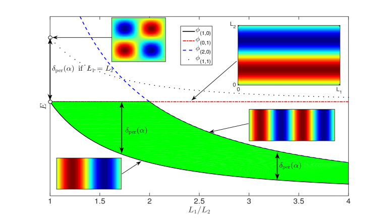
Figure 13: Phase diagram of the first several eigenvalues and their corresponding eigenfunctions of (5.1) with $n=2$, $\alpha=1.5$ and $V_{{}_{\Omega}}(\mathbf{x})\equiv 0$ for different $L_{1}/L_{2}$. Obviously, for different ratios $L_{1}/L_{2}$, the choice of the second excited state $\phi_{2}^{(\alpha)}$ is different. The green part denotes the fundamental gap $\delta_{\rm per}(\alpha)$ for $L_{1}>l_{2}$.

6 Conclusion

By using asymptotic and numerical methods, we obtain the fundamental gaps of the fractional Schrödinger operator (FSO) in different cases including the local FSO on bounded domains, the FSO on bounded domains with zero extension outside the domains, the FSO in the whole space, and the FSO on bounded domains with periodic boundary conditions. Based on our asymptotic and numerical results, we formulate gap conjectures of the fundamental gap of the FSO in different cases. The gap conjectures link the algebraic property – difference of the first two smallest eigenvalues of the eigenvalue problem – and the geometric property – diameters of the bounded domains.

References

• [1] M. Ainsworth, and Z. Mao, Analysis and approximation of a fractional Cahn-Hilliard equation, SIAM J. Numer. Anal., 55 (2017), 1689–1718.
• [2] B. Andrews and J. Clutterbuck, Proof of the fundamental gap conjecture, J. Amer. Math. Soc., 24 (2011), 899–899.
• [3] M. Ashbaugh, The fundamental gap, Workshop on Low Eigenvalues of Laplace and Schrödinger Operators, American Institute of Mathematics, Palo Alto, California (2006).
• [4] M. S. Ashbaugh and R. Benguria, Optimal lower bound for the gap between the first two eigenvalues of one-dimensional Schrödinger operators with symmetric single-well potentials, Proc. Amer. Math. Soc., 105 (1989), 419–424.
• [5] R. A. Askey and A. B. Olde Daalhuis, Generalized hypergeometric function, NIST Handbook of Mathematical Functions, Cambridge University Press, 2010.
• [6] R. Bañuelos and T. Kulczycki, The Cauchy process and the Steklov problem, J. Funct. Anal., 211 (2004), 355–423.
• [7] W. Bao, N. Ben Abdallah and Y. Cai, Gross-Pitaevskii-Poisson equations for dipolar Bose-Einstein condensate with anisotropic confinement, SIAM J. Math. Anal., 44 (2012), pp. 1713-1741.
• [8] W. Bao and Y. Cai, Mathematical theory and numerical methods for Bose-Einstein condensation, Kinet. Relat. Mod., 6 (2013), 1-135.
• [9] W. Bao, H. Jian, N. J. Mauser and Y. Zhang, Dimension reduction of the Schrödinger equation with Coulomb and anisotropic confining potentials, SIAM J. Appl. Math., 73 (2013), 2100-2123.
• [10] W. Bao and F. Y. Lim, Analysis and computation for the semiclassical limits of the ground and excited states of the Gross-Pitaevskii equation, Proc. Sympos. Appl. Math., Amer. Math. Soc., 67 (2009), 195-215.
• [11] W. Bao and X. Ruan, Fundamental gaps of the Gross-Pitaevskii equation with repulsive interaction, arXiv:1512.07123.
• [12] B. Barrios, E. Colorado, A. De Pablo and U. Sanchez, On some critical problems for the fractional Laplacian operator, J. Differential Equations, 252 (2012), 6133–6162.
• [13] A. Bueno-Orovio, D. Kay, and K. Burrage, Fourier spectral methods for fractional-in-space reaction-diffusion equations, BIT, 54 (2014), 937–954.
• [14] X. Cabré, J. Tan, Positive solutions of nonlinear problems involving the square root of the Laplacian, Adv. Math. 224 (2010), 2052–2093.
• [15] L. Caffarelli and L. Silvestre, An extension problem related to the fractional Laplacian, Comm. Partial Differential Equations, 32 (2007), 1245–1260.
• [16] L. Caffarelli and L. Silvestre, Regularity theory for fully nonlinear integro-differential equations, Comm. Pure Appl. Math. 62 (2009), 597–638.
• [17] L. Caffarelli and L. Silvestre, Regularity results for nonlocal equations by approximation, Arch. Ration. Mech. Anal. 200 (2011), 59–88.
• [18] Y. Cai, M. Rosenkranz, Z. Lei and W. Bao, Mean-field regime of trapped dipolar Bose-Einstein condensates in one and two dimensions, Phys. Rev. A, 82 (2010), 043623.
• [19] A. Capella, Solutions of a pure critical exponent problem involving the half-Laplacian in annular-shaped domains, Commun. Pure Appl. Anal., 10 (2011), no. 6, 1645–1662.
• [20] Z. -Q. Chen and R. Song, Two-sided eigenvalue estimates for subordinate processes in domains, J. Funct. Anal., 226 (2005), 90–113.
• [21] A. B. Olde Daalhuis, Hypergeometric function, NIST Handbook of Mathematical Functions, Cambridge University Press, 2010.
• [22] R. D. Deblassie, Higher order PDEs and symmetric stable processes, Probab. Theory Rel., 129 (2004), 495–536.
• [23] S. Duo and Y. Zhang, Computing the ground and first excited states of the fractional Schrödinger equation in an infinite potential well, Commun Comput Phys., 18 (2015), 321–350.
• [24] R. P. Feynman and A.R. Hibbs, Quantum Mechanics and Path Integrals, McGraw-Hill, New York, 1965.
• [25] R.P. Feynman, Statistical Mechanics, Benjamin. Reading, Mass. 1972.
• [26] M. Jeng, S.-L.-Y. Xu, E. Hawkins, and J. M. Schwarz, On the nonlocality of the fractional Schrödinger equation, J. Math. Phys. 51, 062102 (2010).
• [27] Y. Huang, and A. Oberman, Numerical methods for the fractional Laplacian: A finite difference-quadrature approach, SIAM J. Numer. Anal., 52, (2010) 3056–3084.
• [28] M. Ilic, F. Liu, I. Turner, and V. Anh, Numerical approximation of a fractional-in-space diffusion equation, I, Fract. Calc. Appl. Anal., 8, (2005) 323–341.
• [29] M. Ilic, F. Liu, I. Turner, and V. Anh, Numerical approximation of a fractional-in-space diffusion equation (II)–with nonhomogeneous boundary conditions, Fract. Calc. Appl. Anal., 9, (2006) 333–349.
• [30] C. Klein, C. Sparber, and P. Markowich, Numerical study of fractional nonlinear Schrödinger equations, Proc. R. Soc. A 470, (2014).
• [31] M. Kwaśnicki, Eigenvalues of the fractional Laplace operator in the interval, J. Funct. Anal., 262 (2012), 2379–2402.
• [32] N. Laskin, Fractional quantum mechanics and Lévy path integrals, Phys. Lett. A, 268 (2000), 298–305.
• [33] N. Laskin, Fractional quantum mechanics, Phys. Rev. E, 62 (2000), 3135–3145.
• [34] N. Laskin, Fractional Schrödinger equation, Phys. Rev. E 66 (2002), 056108.
• [35] Z. Mao and J. Shen, Hermite Spectral Methods for Fractional PDEs in Unbounded Domains, SIAM J. Sci. Comput., 39 (2017), 1928–1950.
• [36] E. Di Nezza, G. Palatucci and E. Valdinoci, Hitchhiker’s guide to the fractional Sobolev spaces, Bull. Sci. Math., 136 (2012), 521–573.
• [37] I. Podlubny, Fractional Differential Equations, Academic Press, 1999.
• [38] L. Roncal and P. R. Stinga, Fractional Laplacian on the torus, Commun. Contemp. Math. 18 (2016), 1550033.
• [39] L. Roncal and P. R. Stinga, Transference of fractional Laplacian regularity, In: Georgakis C., Stokolos A., Urbina W. (eds) Special Functions, Partial Differential Equations, and Harmonic Analysis. Springer Proc. Math. Stat., 108. Springer, Cham, 2014.
• [40] S. G. Samko, A. A. Kilbas, and O. I. Maritchev, Fractional Integrals and Derivatives, Gordon and Breach, New York, 1993.
• [41] R. Servadei and E. Valdinoci, On the spectrum of two different fractional operators, Proceedings of the Royal Society of Edinburgh: Section A Mathematics, 144 (2014), 831–855.
• [42] C. Sheng, J. Shen and D. Cao, Solving PDEs with Fractional Laplacian by using Fourierization of the Legendre-Galerkin method, submitted.
• [43] C. Sheng and J. Shen, Fourierization of Mapped Chebyshev spectral method for Fractional PDEs in unbounded domains, submitted.
• [44] I. Singer, B. Wong, S.-T. Yau and S. S.-T. Yau, An estimate of the gap of the first two eigenvalues in the Schrödinger operator, Ann. Sc. Norm. Super. Pisa Cl. Sci. (4), 12 (1985), 319–333.
• [45] P. R. Stinga, Fractional powers of second order partial differential operators: extension problem and regularity theory, PhD thesis, Universidad Autónoma de Madrid, Madrid (2010).
• [46] J. Tan, The Brezis-Nirenberg type problem involving the square root of the Laplacian, Calc. Var. Partial Differential Equations, 36 (2011), 21–41.
• [47] A. Zoia, A. Rosso, and M. Kardar, Fractional Laplacian in bounded domains, Phys. Rev. E 76 (2007), 021116.