Abstract

Submodular extensions of an energy function can be used to efficiently compute approximate marginals via variational inference. The accuracy of the marginals depends crucially on the quality of the submodular extension. To identify the best possible extension, we show an equivalence between the submodular extensions of the energy and the objective functions of linear programming (LP) relaxations for the corresponding MAP estimation problem. This allows us to (i) establish the worst-case optimality of the submodular extension for Potts model used in the literature; (ii) identify the worst-case optimal submodular extension for the more general class of metric labeling; and (iii) efficiently compute the marginals for the widely used dense CRF model with the help of a recently proposed Gaussian filtering method. Using synthetic and real data, we show that our approach provides comparable upper bounds on the log-partition function to those obtained using tree-reweighted message passing (TRW) in cases where the latter is computationally feasible. Importantly, unlike TRW, our approach provides the first practical algorithm to compute an upper bound on the dense CRF model.

1 Introduction

The desirable optimization properties of submodular set functions have been widely exploited in the design of approximate MAP estimation algorithms for discrete conditional random fields (CRFs) [Boykov et al.,, 2001; Kumar et al.,, 2011]. Submodularity has also been recently used to design an elegant variational inference algorithm to compute the marginals of a discrete CRF by minimising an upper-bound on the log-partition function. In the initial work of [Djolonga and Krause,, 2014], the energy of the CRF was restricted to be submodular. In a later work  [Zhang et al.,, 2015], the algorithm was extended to handle more general Potts energy functions. The key idea here is to define a large ground set such that its subsets represent valid labelings, sublabelings or even incorrect labelings (these may assign two separate labels to a random variable and hence be invalid). Given the large ground set, it is possible to define a submodular set function whose value is equal to the energy of the CRF for subsets that specify a valid labeling of the model. We refer to such a set function as a submodular extension of the energy.

For a given energy function, there exists a large number of possible submodular extensions. The accuracy of the variational inference algorithm depends crucially on the choice of the submodular extension. Yet, previous work has largely ignored the question of identifying the best extension. Indeed, the difficulty of identifying submodular extensions of general energy functions could be a major reason why the experiments of [Zhang et al.,, 2015] were restricted to the special case of models specified by the Potts energy functions.

In this work, we establish a hitherto unknown connection between the submodular extension of the Potts model proposed by Zhang et al., [2015], and the objective function of an accurate linear programming (LP) relaxation of the corresponding MAP estimation problem [Kleinberg and Tardos,, 2002]. This connection has three important practical consequences. First, it establishes the accuracy of the submodular extension of the Potts model, via the UGC-hardness worst-case optimality of the LP relaxation. Second, it provides an accurate submodular extension of the hierarchical Potts model, via the LP relaxation of the corresponding MAP estimation problem proposed by Kleinberg and Tardos, [2002]. Since any metric can be accurately approximated as a mixture of hierarchical Potts models [Bartal,, 1996, 1998], this result also provides a computationally feasible algorithm for estimating the marginals for metric labeling. Third, it establishes the equivalence between the subgradient of the LP relaxation and the conditional gradient of the problem of minimising the upper bound of the log-partition. This allows us to employ the widely used dense CRF, since the subgradient of its LP relaxation can be efficiently computed using a recently proposed modified Gaussian filtering algorithm [Ajanthan et al.,, 2017]. As a consequence, we provide the first efficient algorithm to compute an upper bound of the log-partition function of dense CRFs. This provides complementary information to the popular mean-field inference algorithm for dense CRFs, which computes a lower bound on the log-partition  [Koltun and Krahenbuhl,, 2011]. We show that the quality of our solution is comparable to tree reweighted message passing (TRW)  [Wainwright et al.,, 2005] for the case of sparse CRFs. Unlike our approach, TRW is computationally infeasible for dense CRFs, thereby limiting its use in practice. Using dense CRF models, we perform stereo matching on standard data sets and obtain better results than [Koltun and Krahenbuhl,, 2011]. The complete code is available at https://github.com/pankajpansari/denseCRF.

2 Preliminaries

We now introduce the notation and definitions that we will make use of in the remainder of the paper.

Submodular Functions

Given a ground set $U=\left\{1,\dots,N\right\}$, denote by $2^{U}$ its power set. A set function $F:2^{U}\to\mathbb{R}$ is submodular if, for all subsets $A,B\subseteq U$, we have

$$F(A\cup B)+F(A\cap B)\leq F(A)+F(B).$$ (1)

The set function $F$ is modular if there exists ${\bf s}\in\mathbb{R}^{N}$ such that $F(A)=\sum_{k\in A}s_{k}\ \forall\ A\subseteq 2^{U}$. Henceforth, we will use the shorthand $s(A)$ to denote ${\sum_{k\in A}}s_{k}$.

Extended Polymatroid

Associated with any submodular function $F$ is a special polytope known as the extended polymatroid defined as

$$EP(F) =\{{\bf s}\in\mathbb{R}^{N}|\enskip\forall A\subseteq U:s(A)\leq F(A)\},$$ (2)

where $\bf s$ denotes the modular function $s(.)$ considered as a vector.

Lovasz Extension

For a given set function $F$ with $F(\emptyset)=0$, the value of its Lovasz extension $f({\bf w}):\mathbb{R}^{N}\to\mathbb{R}$ is defined as follows: order the components of $\bf w$ in decreasing order such that $w_{j_{1}}\geq w_{j_{2}}\geq\dots\geq w_{j_{N}}$, where $(j_{1},j_{2},\dots,j_{N})$ is the corresponding permutation of the indices. Then,

$$f({\bf w})=\sum_{k=1}^{N}w_{j_{k}}\left(F(j_{1},\dots,j_{k})-F(j_{1},\dots,j_{k-1})\right).$$ (3)

The function $f$ is an extension because it equals $F$ on the vertices of the unit cube. That is, for any $A\subseteq V$, $f({\bf 1}_{A})=F(A)$ where ${\bf 1}_{A}$ is the $0\mathchar 45\relax{1}$ indicator vector corresponding to the elements of $A$.

Property 1.

By Edmond’s greedy algorithm [Edmonds,, 1970], if ${\bf w}\geq 0$ (non-negative elements),

$$f({\bf w})=\max_{{\bf s}\in EP(F)}\langle{\bf w},{\bf s}\rangle.$$ (4)

Property 4 implies that an LP over $EP(F)$ can be solved by computing the value of the Lovasz extension using equation (3).

Property 2.

The Lovasz extension $f$ of a submodular function $F$ is a convex piecewise linear function.

Property 2 holds since $f({\bf w})$ is the pointwise maximum of linear functions according to equation (4).

CRF and Energy Functions

A CRF is defined as a graph on a set of random variables ${\mathcal{X}}=\{X_{1},\dots,X_{N}\}$ related by a set of edges $\mathcal{N}$. We wish to assign every variable $X_{a}$ one of the labels from the set $\mathcal{L}=\{1,2,\dots,L\}$. The quality of a labeling $\bf x$ is given by an energy function defined as

$$E({\bf x})=\sum_{a\in{\mathcal{X}}}\phi_{a}(x_{a})+\sum_{(a,b)\in{\mathcal{N}}}\phi_{ab}(x_{a},x_{b}),$$ (5)

where $\phi_{a}$ and $\phi_{ab}$ are the unary and pairwise potentials respectively. In computer vision, we often think of $\mathcal{X}$ as arranged on a grid. A sparse CRF has $\mathcal{N}$ defined by 4-connected or 8-connected neighbourhood relationships. In a dense CRF, on the other hand, every variable is connected to every other variable.

The energy function also defines a probability distribution $P({\bf x})$ as follows:

$$P({\bf x})=\begin{cases}\frac{1}{\mathcal{Z}}\exp(-E({\bf x}))&\quad\text{if}\enskip{\bf x}\in{\mathcal{L}}^{N},\\ 0&\quad\text{otherwise}.\\ \end{cases}$$ (6)

The normalization factor $Z=\sum_{{\bf x}\in{\mathcal{L}}^{N}}\exp(-E({\bf x}))$ is known as the partition function.

Inference

There are two types of inference problems in CRFs:

(i) Marginal inference: We want to compute the marginal probabilities $P(X_{a}=i)$ for every $a=1,2,\dots,N$ and $i=1,2,\dots,L$.

(ii) MAP inference: We want to find a labeling with the minimum energy, that is, $\min_{{\bf x}\in{\mathcal{L}}^{N}}E({\bf x})$. Equivalently, MAP inference finds the mode of $P({\bf x})$.

3 Review: Variational Inference Using Submodular Extensions

We now summarise the marginal inference method of Zhang et al., [2015]. To do this, we need to first define submodular extensions.

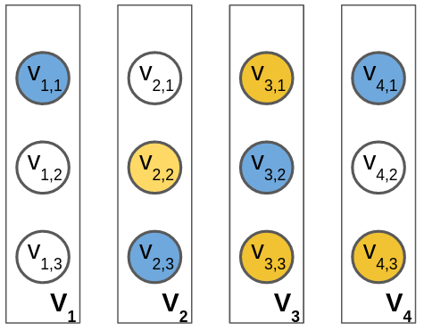
Figure 1: Illustration of $1$-of-$L$ encoding used in [Zhang et al.,, 2015] with 4 variables and 3 labels. The blue labeling, corresponding to $X_{1}=1,X_{2}=3,X_{3}=2,X_{4}=1$, is valid. The yellow labeling, corresponding to $X_{2}=2,X_{3}=1,3,X_{4}=3$, is invalid since $X_{3}$ has been assigned multiple labels and $X_{1}$ has been assigned none.

Submodular Extensions

A submodular extension is defined using a ground set such that some of its subsets correspond to valid CRF labelings. To such an extension, we need an encoding scheme which gives the sets corresponding to valid CRF labelings.

One example of an encoding scheme is the $1$-of-$L$ encoding, illustrated in figure 1. Let each variable $X_{a}$ take one of $L$ possible labels. In this scheme, we represent the set of possible assignments for $X_{a}$ by the set $V_{a}=\{v_{a1},v_{a2},\dots,v_{aL}\}$. If $X_{a}$ is assigned label $i$, then we select the element $v_{ai}$. Extending to all variables, our ground set becomes $V=\cup_{a=1}^{N}V_{a}$. A valid assignment $A\subseteq V$ assigns each variable exactly one label, that is, $|A\cap V_{a}|=1$ for all $V_{a}$. We denote the set of valid assignments by $\mathcal{M}$ where $\mathcal{M}=\cap_{a=1}^{N}\mathcal{M}_{a}$ and $\mathcal{M}_{a}=\{A:|A\cap V_{a}|=1\}$.

Using our ground set $V$, we can define a submodular function $F$ which equals $E(\bf x)$ for all sets corresponding to valid labelings, that is, $F(A_{\bf x})=E({\bf x}),\ {\bf x}\in{\mathcal{L}}^{N}$ where $A_{\bf x}$ is the set encoding of $\bf x$. We call such a function $F$ a submodular extension of $E({\bf x})$.

Upper-Bound on Log-Partition

Using a submodular extension $F$ and given any ${\bf s}\in EP(F)$, we can obtain an upper-bound on the partition function as

$${\mathcal{Z}}=\sum_{A\in{\mathcal{M}}}\exp(-F(A))\leq\sum_{A\in{\mathcal{M}}}\exp(-s(A)),$$ (7)

where $\mathcal{M}$ is the set of valid labelings. The upper-bound is the partition function of the distribution $Q(A)\propto\exp(-s(A))$, which factorises fully because $s(.)$ is modular. Since ${\bf s}\in EP(F)$ is a free parameter, we can obtain good approximate marginals of the distribution $P(\cdot)$ by minimising the upper-bound. After taking logs, we can equivalently write our optimisation problem as

$$\min_{{\bf s}\in EP(F)}g({\bf s}),\text{where }g({\bf s})=\log\sum_{A\in{\mathcal{M}}}\exp(-s(A)).$$ (8)

Conditional Gradient Algorithm

The conditional gradient algorithm (algorithm 1) [Frank and Wolfe,, 1956] is a good candidate for solving problem (8) due to two reasons. First, problem (8) is convex. Second, as solving an LP over EP(F) is computationally tractable (property 4), the conditional gradient can be found efficiently. The algorithm starts with an initial solution $\bf s_{0}$ (line 1). At each iteration, we compute the conditional gradient $\bf s^{*}$ (line 3), which minimises the linear approximation $g({\bf s}_{k})+\nabla g({\bf s}_{k})^{T}({\bf s}-{\bf s}_{k})$ of the objective function. Finally, $\bf s$ is updated by either (i) fixed step size schedule, as in line 7 of algorithm 1, or (ii) by doing line search ${\bf s}_{k+1}=\min_{0\leq\gamma\leq 1}g(\gamma{\bf s}^{*}+(1-\gamma){\bf s}_{k})$.

Algorithm 1 Upper Bound Minimisation using Conditional Gradient Descent

1:  Initialize ${\bf s}={\bf s}_{0}\in EP(F)$

2:  for k = 1 to MAX_ITER do

3:     ${\bf s^{*}}=\operatorname*{argmin}_{{\bf s}\in EP(F)}\langle\nabla g({\bf s}_{k}),{\bf s}\rangle$

4:     if $\langle{\bf s^{*}-s}_{k},\nabla g({\bf s}_{k})\rangle\leq\epsilon$ then

5:        break

6:     end if

7:     ${\bf s}_{k+1}={\bf s}_{k}+\gamma({\bf s^{*}}-{\bf s}_{k})$ with $\gamma=2/(k+2)$

8:  end for

9:  return  $\bf s$

4 Worst-case Optimal Submodular Extensions via LP Relaxations

Worst-case Optimal Submodular Extensions

Different choices of extensions $F$ change the domain in problem (8), leading to different upper bounds on the log-partition function. How does one come up with an extension which yields the tightest bound?

In this paper, we focus on submodular extension families $\mathcal{F}(.)$ which for each instance of the energy function $E(.)$ belonging to a given class $\mathcal{E}$ gives a corresponding submodular extension ${\mathcal{F}}(E)$. We find the extension family ${\mathcal{F}}_{opt}$ that is worst-case optimal. This implies that there does not exist another submodular extension family ${\mathcal{F}}$ that gives a tighter upper bound for problem (8) than ${\mathcal{F}}_{opt}$ for all instances of the energy function in $\mathcal{E}$. Formally,

$$\nexists{\mathcal{F}}:\min_{{\bf s}\in EP({\mathcal{F}}(E))}g({\bf s})\leq\min_{{\bf s}\in EP({\mathcal{F}}_{opt}(E))}g({\bf s})\enspace\forall\;E(.)\in\mathcal{E}.$$ (9)

Note that our problem is different from taking a given energy model and obtaining a submodular extension which is optimal for that model. Also, we seek a closed-form analytical expression for $\mathcal{F}$. For the sake of clarity, in the analysis that follows we use $F$ to represent ${\mathcal{F}}(E)$ where the meaning is clear from context. The two classes of energy functions we consider in this paper are Potts and hierarchical Potts families.

Using LP Relaxations

If we introduce a temperature parameter in $P({\bf x})$ (equation (6)) by using $E({\bf x})/T$ and decrease $T$, the resulting distribution starts to peak more sharply around its mode. As $T\to 0$, marginal estimation becomes the same as MAP inference since the resulting distribution $P^{0}({\bf x})$ has mass 1 at its mode ${\bf x}^{*}$ and is 0 everywhere else. Given the MAP solution ${\bf x}^{*}$, one can compute the marginals as $P(X_{i}=j)=[x_{i}^{*}=j]$, where [.] is the Iverson bracket.

Motivated by this connection, we ask if one can introduce a temperature parameter to our problem (8) and transform it to an LP relaxation in the limit $T\to 0$? We can then hope to use the tightest LP relaxations of MAP problems known in literature to find worst-case optimal submodular extensions. We answer this question in affirmative. Specifically, in the following two sections we show how one can select the set encoding and submodular extension to convert problem (8) to the tightest known LP relaxations for Potts and hierarchical Potts models. Importantly, we prove the worst-case optimality of the extensions thus obtained.

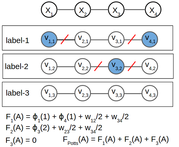
Figure 2: An illustration of the worst-case optimal submodular extension for Potts model for a chain graph of 4 variables, each of which can take 3 labels. The figure shows the way to compute the extension values of the set $A=\{v_{1,1},v_{4,1},v_{3,2}$}.

5 Potts Model

The Potts model, also known as the uniform metric, specifies the pairwise potentials $\phi_{ab}(x_{a},x_{b})$ in equation (5) as follows:

$$\phi_{ab}(x_{a},x_{b})=w_{ab}\cdot[x_{a}\neq x_{b}],$$ (10)

where $w_{ab}$ is the weight associated with edge $(a,b)$.

Tightest LP Relaxation

Before describing our set encoding and submodular extension, we briefly outline the LP relaxation of the corresponding MAP estimation problem. To this end, we define indicator variables $y_{ai}$ which equal 1 if $X_{a}=i$, and 0 otherwise. The following LP relaxation is the tightest known for Potts model in the worst-case, assuming the Unique Games Conjecture to be true [Manokaran et al.,, 2008]

$$\text{(P-LP)}\quad\min_{\bf y}\enskip E({\bf y})=\sum_{a}\sum_{i}\phi_{a}(i)y_{ai}+$$

$$\sum_{(a,b)\in{\mathcal{N}}}\sum_{i}\frac{w_{ab}}{2}\cdot|y_{ai}-y_{bi}|$$

s.t $${\bf y}\in\Delta.$$ (11)

The set $\Delta$ is the union of $N$ probability simplices:

$$\Delta=\{{\bf y}_{a}\in\mathbb{R}^{L}|{\bf y}_{a}\geq 0\textrm{ and }\langle{\bf 1},{\bf y}_{a}\rangle=1\},$$ (12)

where $\bf y$ is the vector of all variables and ${\bf y}_{a}$ is the component of $\bf y$ corresponding to $X_{a}$.

Set Encoding

We choose to use the $1$-of-$L$ encoding for Potts model as described in section 3. With the encoding scheme for Potts model above, $g({\bf s})$ can be factorised and problem (8) can be rewritten as:

$$\min_{{\bf s}\in EP(F)}\quad\sum_{a=1}^{N}\log\sum_{i=1}^{L}\exp(-s_{ai}).$$ (13)

(See Remark 1 in appendix)

Marginal Estimation with Temperature

We now introduce a temperature parameter $T>0$ to problem (13) which divides $E({\bf x})$, or equivalently divides $\bf s$ belonging to $EP(F)$. Also, since $T>0$, we can multiply the objective by $T$ leaving the problem unchanged. Without changing the solution, we can transform problem (13) as follows

$$\min_{{\bf s}\in EP(F)}\quad g_{T}({\bf s})=\sum_{a=1}^{N}T\cdot\log\sum_{i=1}^{L}\exp(-\frac{s_{ai}}{T}).$$ (14)

Worst-case Optimal Submodular Extension

We now connect our marginal estimation problem (8) with LP relaxations using the following proposition.

Proposition 1.

Using the $1$-of-$L$ encoding scheme, in the limit $T\to 0$, problem (34) for Potts model becomes:

$$-\min_{{\bf y}\in\Delta}f({\bf y})$$ (15)

where $f(.)$ is the Lovasz extension of $F(.)$.
(Proof in appendix)

The above problem is equivalent to an LP relaxation of the corresponding MAP estimtation problem (see Remark 2 in appendix). We note that $g_{T}({\bf s})$ in problem (34) becomes the objective function of an LP relaxation in the limit $T\to 0$. We seek to obtain the worst-case optimal submodular extension by making $g_{T}({\bf s})$ same as the objective of (P-LP) as $T\to 0$. Since at $T=1$, problems (34) and (13) are equivalent, this gives us the worst-case optimal extension for our problem (13) as well.

The question now becomes how to recover the worst-case optimal submodular extension using $E({\bf y})$. The following propositions answers this question.

Proposition 2.

The worst-case optimal submodular extension for Potts model is given by $F_{Potts}(A)=\sum_{i=1}^{L}F_{i}(A)$, where

$$F_{i}(A) =\sum_{a}\phi_{a}(i)[|A\cap\{v_{ai}\}|=1]+$$

$$\sum_{(a,b)\in{\mathcal{N}}}\frac{w_{ab}}{2}\cdot[|A\cap\{v_{ai},v_{bi}\}|=1]$$ (16)

Also, $E({\bf y})$ in (P-LP) is the Lovasz extension of $F_{Potts}$. (Proof in appendix)

Proposition 2 paves the way for us to identify the worst-case optimal extension for hierarchical Potts model, which we discuss in the following section.

Figure 3: An st-graph specifying the worst-case optimal submodular extension for Potts model for 2 variables with 3 labels each and connected to each other. There is a node for each variable and each label, that is, for all elements of the ground set. The nodes have been labeled as ‘variable-label’, hence node 1-1 represents the element $v_{11}$ and so on. The solid blue arcs model the unary potentials, and the dotted red arcs represent the pairwise potentials. Each dotted red arc has weight $w_{12}/2$.

6 Hierarchical Potts

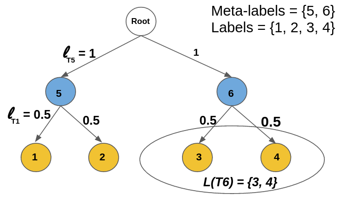
Figure 4: An hierarchical Potts model instance illustrating notations with 2 meta-labels (blue) and 4 labels (yellow). All labels are at the same level. $r=2$, that is, edge-length decreases by 2 at each level. Also, distance between labels 1 and 3 is $d(1,3)=0.5+1+1+0.5=3$.

Potts model imposes the same penalty for unequal assignment of labels to neighbouring variables, regardless of the label dissimilarity. A more natural approach is to vary the penalty based on how different the labels are. A hierarchical Potts model permits this by specifying the distance between labels using a tree with the following properties:

1. The vertices are of two types: (i) the leaf nodes representing labels, and (ii) the non-leaf nodes, except the root, representing meta-labels.

2. The lengths of all the edges from a parent to its children are the same.

3. The lengths of the edges along any path from the root to a leaf decreases by a factor of at least $r\geq 2$ at each step.

4. The metric distance between nodes of the tree is the sum of the edge lengths on the unique path between them.

A subtree $T$ of an hierarchical Potts model is a tree comprising all the descendants of some node $v$ (not root). Given a subtree $T$, $l_{T}$ denotes the length of the tree-edge leading upward from the root of $T$ and $L(T)$ denotes the set of leaves of $T$. We call the leaves of the tree as labels and all other nodes of the tree expect the root as meta-labels. Figure 4 illustrates the notations in the context of a hierarchical Potts model.

Tightest LP Relaxation

We use the same indicator variables $y_{ai}$ that were employed in the LP relaxation of Potts model. Let $y_{a}(T)=\sum_{i\in L(T)}y_{ai}$. The following LP relaxation is the tightest known for hierarchical Potts model in the worst-case, assuming the Unique Games Conjecture to be true [Manokaran et al.,, 2008]

$$\text{(T-LP)}\quad\min_{\bf y}\enskip \widetilde{E}({\bf y})=\sum_{a}\sum_{i}\phi_{a}(i)y_{ai}+$$

$$\sum_{(a,b)\in{\mathcal{N}}}w_{ab}\sum_{T}l_{T}\cdot|y_{a}(T)-y_{b}(T)|$$

such that $${\bf y}\in\Delta.$$ (17)

The set $\Delta$ is the same domain as defined in equation (57). We rewrite this LP relaxation using indicator variables $z_{ai}$ for all labels and meta-labels as

(T-LP-FULL) $$\quad\min\widetilde{E}({\bf z})$$

$$\text{such that}\quad{\bf z}\in\Delta^{\prime}$$ (18)

where $\Delta^{\prime}$ is the convex hull of the vectors satisfying

$$\sum_{i\in\mathcal{L}}z_{ai}=1,\enskip z_{ai}\in\{0,1\}\enskip\forall a\in{\mathcal{X}},i\in\mathcal{L}$$ (19)

and $$z_{ai}=\sum_{j\in L(T_{i})}z_{aj}.\enskip\forall a\in{\mathcal{X}},i\in\mathcal{R-L}$$ (20)

The details of the new relaxation (T-LP-FULL) can be found in the appendix.

Set Encoding

For any variable $X_{a}$, let the set of possible assignment of labels and meta-labels be the set $V_{a}=\{v_{a1},\dots,v_{aM}\}$, where $M$ is the total number of nodes in the tree except the root. Our ground set is $V=\cup_{a=1}^{N}V_{a}$ of size $N\cdot M$.

A consistent labeling of a variable assigns it one label, and all meta-labels on the path from root to the label. Let us represent the set of consistent assignments for $X_{a}$ by the set $P_{a}=\{p_{a1},\dots,p_{aL}\}$, where $p_{ai}$ is the collection of elements from $V_{a}$ for label $i$ and all meta-labels on the path from root to label $i$.

The set of valid labelings $A\subseteq V$ assigns each variable exactly one consistent label. This constraint can be formally written as $\mathcal{M}=\cap_{a=1}^{N}\mathcal{M}_{a}$ where $\mathcal{M}_{a}$ has exactly one element from $P_{a}$.

Let $s^{\prime}_{ai}$ be the sum of the components of $\bf s$ corresponding to the elements of $p_{ai}$, that is,

$$s^{\prime}_{ai}=\sum_{t\in p_{ai}}s_{t}.$$ (21)

Using our encoding scheme, we rewrite problem (8) as:

$$\min_{{\bf s}\in EP(F)}\quad\sum_{a=1}^{N}\log\sum_{i=1}^{L}\exp(-s^{\prime}_{ai}).$$ (22)

Marginal Estimation with Temperature

Similar to Potts model, we now introduce a temperature parameter $T>0$ to problem (22). The transformed problem becomes

$$\min_{{\bf s}\in EP(F)}\quad g_{T}({\bf s})=\sum_{a=1}^{N}T\cdot\log\sum_{i=1}^{L}\exp(-\frac{s^{\prime}_{ai}}{T}).$$ (23)

Worst-case Optimal Submodular Extension

The following proposition connects the marginal estimation problem (8) with LP relaxations:

Proposition 3.

In the limit $T\to 0$, problem (52) for hierarchical Potts energies becomes:

$$-\min_{{\bf z}\in\Delta^{\prime}}f({\bf z})$$ (24)

(Proof in appendix).

The above problem is equivalent to an LP relaxation of the corresponding MAP estimtation problem (see Remark 3 in appendix). Hence, $g_{T}({\bf s})$ becomes the objective function of an LP relaxation in the limit $T\to 0$. We seek to make this objective same as $\widetilde{E}({\bf z})$ of (T-LP-FULL) in the limit $T\to 0$. The question now becomes how to recover the worst-case optimal submodular extension from $\widetilde{E}({\bf z})$.

Proposition 4.

The worst-case optimal submodular extension for hierarchical Potts model is given by $F_{hier}(A)=\sum_{i=1}^{M}F_{i}(A)$, where

$$F_{i}(A) =\sum_{a}\phi^{\prime}_{a}(i)[|A\cap\{v_{ai}\}|=1]+$$

$$\sum_{(a,b)\in{\mathcal{N}}}{w_{ab}}\cdot l_{T_{i}}\cdot[|A\cap\{v_{ai},v_{bi}\}|=1]$$ (25)

Also, $\widetilde{E}({\bf z})$ in (T-LP-FULL) is the Lovasz extension of $F_{hier}$.

(Proof in appendix)

Since any finite metric space can be probabilistically approximated by mixture of tree metric [Bartal,, 1996], the worst-case optimal submodular extension for metric energies can be obtained using $F_{hier}$. Note that $F_{hier}$ reduces to $F_{Potts}$ for Potts model. One can see this by considering the Potts model as a star-shaped tree with edge weights as 0.5.

7 Fast Conditional Gradient Computation for Dense CRFs

Dense CRF Energy Function

A dense CRF is specified by the following energy function

$$E({\bf x})=\sum_{a\in{\mathcal{X}}}\phi_{a}(x_{a})+\sum_{a\in{\mathcal{X}}}\sum_{b\in{\mathcal{X}},b\neq a}\phi_{ab}(x_{a},x_{b}).$$ (26)

Note that every random variable is a neighbour of every other random variable in a dense CRF. Similar to previous work [Koltun and Krahenbuhl,, 2011], we consider the pairwise potentials to be to be Gaussian, that is,

$$\phi(i,j)=\mu(i,j)\sum_{m}w^{(m)}k({\bf f}_{a}^{(m)},{\bf f}_{b}^{(m)}),$$ (27)

$$k({\bf f}_{a}^{(m)},{\bf f}_{b}^{(m)})=\exp\left(\frac{-||{\bf f}_{a}-{\bf f}_{b}||^{2}}{2}\right).$$ (28)

The term $\mu(i,j)$ is known as label compatibility function between labels $i$ and $j$. Potts model and hierarchical Potts models are examples of $\mu(i,j)$. The other term is a mixture of Gaussian kernels $k(.,.)$ and is called the pixel compatibility function. The terms ${\bf f}_{a}^{(m)}$ are features that describe the random variable $X_{a}$. In practice, similar to [Koltun and Krahenbuhl,, 2011], we use $x,y$ coordinates and RGB values associated to a pixel as its features.

Algorithm 1 assumes that the conditional gradient $\bf s^{*}$ in step 3 can be computed efficiently. This is certainly not the case for dense CRFs, since computing $s^{*}$ involves $NL$ function evaluations of the submodular extension $F$, where $N$ is the number of variables, and $L$ is the number of labels. Each $F$ evaluation has complexity ${\mathcal{O}}(N)$ using the efficient Gaussian filtering algorithm of [Koltun and Krahenbuhl,, 2011]. However, computation of $s^{*}$ would still be ${\mathcal{O}}(N^{2})$ this way, which is clearly impractical for computer-vision applications where $N\sim 10^{5}-10^{6}$.

However, using the equivalence of relaxed LP objectives and the Lovasz extension of submodular extensions in proposition 6, we are able to compute $s^{*}$ in ${\mathcal{O}}(NL)$ time. Specifically, we use the algorithm of Ajanthan et al., [2017], which provides an efficient filtering procedure to compute the subgradient of the LP relaxation objective $E({\bf y})$ of (P-LP).

Proposition 5.

Computing the subgradient of $E({\bf y})$ in (P-LP) is equivalent to computing the conditional gradient for the submodular function $F_{Potts}$.

(Proof in appendix).

A similar observation can be made in case of hierarchical Potts model. Hence we have the first practical algorithm to compute upper bound of log-partition function of a dense CRF for Potts and metric energies.

8 Experiments

Using synthetic data, we show that our upper-bound compares favorably with TRW for both Potts and hierarchical Potts models. For comparison, we restrict ourselves to sparse CRFs, as the code available for TRW does not scale well to dense CRFs. We also perform stereo matching using dense CRF models and compare our results with the mean-field-based approach of [Koltun and Krahenbuhl,, 2011]. All experiments were run on a x86-64, 3.8GHz machine with 16GB RAM. In this section, we refer to our algorithm as Submod and mean field as MF.

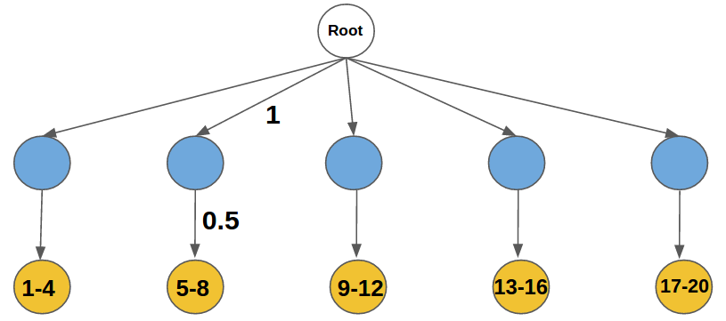
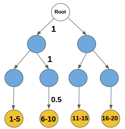
(a) Tree 1	(b) Tree 2

Figure 5: The hierarchical Potts models defining pairwise distance among 20 labels used for upper-bound comparison with TRW. Blue nodes are the meta-labels and yellow nodes are labels. All the edges at a particular level have the same edge weights. The sequence of weights from root level to leaf level is 1, 0.5 for tree 1 and 1, 1, 0.5 for tree 2. The yellow node is shown to clump together 4 and 5 leaf nodes for tree 1 and 2 respectively.

Figure 6: An st-graph specifying the alternate submodular extension for Potts model for 2 variables with 3 labels each and connected to each other. The convention used is same as in figure 3. Each dotted red arc has weight $w_{12}/2$. This alternate extension was also used to derive the extension for hierarchical Potts model.

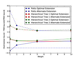
Figure 7: Upper-bound comparison using synthetic data. The plot shows the ratio (Submod bound - TRW bound)/|TRW bound| averaged over 100 unary instances as a function of pairwise weights using the worst-case optimal and alternate extension for Potts and hierarchical Potts models. We observe that the worst-case optimal extension (solid) results in tighter bounds as compared to the respective alternate extensions (dotted). Also, the worst-case optimal extension bounds are in similar range as the TRW bounds. Figure best viewed in color.

8.1 Upper-bound Comparison using Synthetic Data

Data

We generate lattices of size 100 $\times$ 100, where each lattice point represents a variable taking one of 20 labels. The pairwise relations of the sparse CRFs are defined by 4-connected neighbourhoods. The unary potentials are uniformly sampled in the range [0, 10]. We consider (a) Potts model and (b) hierarchical Potts models with pairwise distance between labels given by the trees of figure 5. The pairwise weights are varied in the range $\{1,2,5,10\}$. We compare the results of our worst-case optimal submodular extension with an alternate submodular extension as given in figure 2.

Method

For our algorithm, we use the standard schedule $\gamma=2/(k+2)$ to obtain step size $\gamma$ at iteration $k$. We run our algorithm till convergence - 100 iterations suffice for this. The experiments are repeated for 100 randomly generated unaries for each model and each weight. For TRW, we used the MATLAB toolbox of [Domke,, 2013]. The baseline code does not optimise over tree distributions. We varied the edge-appearance probability in trees over the range [0.1 - 0.5] and found 0.5 to give tightest upper bound.

Results

We plot the ratio of the normalised difference of the upper bound values of our method with TRW as a function of pairwise weights. The ratios are averaged over 100 instances of unaries. Figure 7 shows the plots for Potts and hierarchical Potts models for the worst-case optimal and alternate extension. We find that the optimal extension (solid) results in tighter upper-bounds than the alternate extension (dotted) for both models. To see the reason for this, we observe that the representation of the submodular function using figure 6 necessitates that $\phi_{a}(i)$ be non-negative. This implies that $F(A)$ values are larger for the worst-case optimal extension of figure 3 as compared to the alternate extension. Hence the minimisation problem 8 has the same objective function $g({\bf s})$ for both cases but the domain $EP(F)$ of equation (2) is larger for the optimal extension, thereby resulting in better minima.

Figure 7 also indicates that our algorithm with optimal extension provides similar range of upper bound as TRW, thereby providing empirical justification of our method. Note that the TRW upper bound has to be tighter than our method. This is because the TRW makes use of the standard LP relaxation [Chekuri et al.,, 2004] which involves marginal variables for nodes as well as edges. On the other hand, our method makes use of the LP relaxation proposed by Kleinberg and Tardos, [2002] which involves marginal variables only for nodes. The standard LP relaxation is tighter than Kleinberg-Tardos relaxation, and hence TRW results in better approximation. However, TRW does not scale well with neighborhood size, thereby prohibiting its use in dense CRFs.

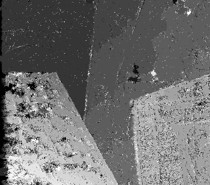
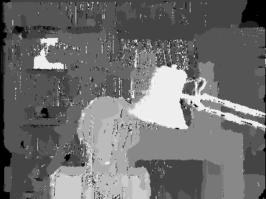
(a) Venus GT	(b) MF solution	(c) Submod solution	(a) Tsukuba GT	(b) MF solution	(c) Submod solution
	60.32s, 1.83e+07	469.75s, 1.55e+07		14.93s, 8.21e+06	215.22s, 4.12e+06
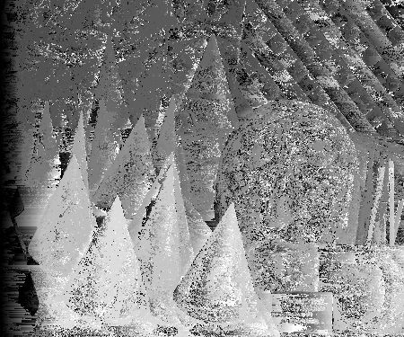
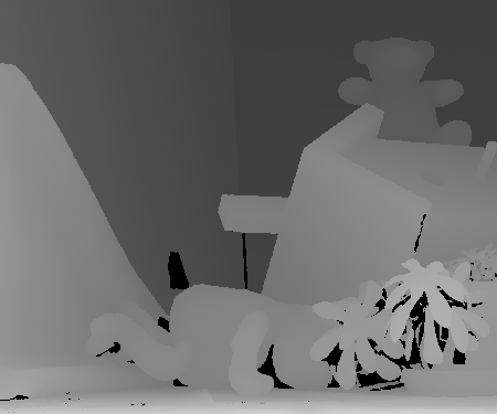
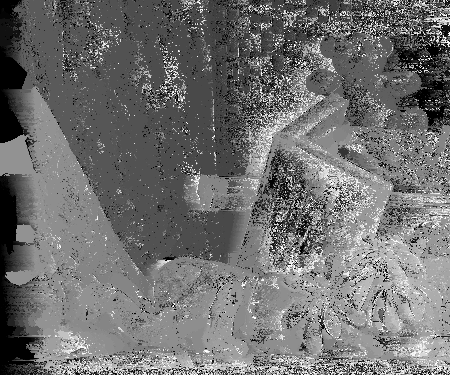
(a) Cones GT	(b) MF solution	(c) Submod solution	(a) Teddy GT	(b) MF solution	(c) Submod solution
	239.14s, 2.68e+07	1082.72s, 1.27e+07		555.30s, 2.36e+07	1257.86s, 1.58e+07

Figure 8: Stereo matching using dense CRFs with Potts compatibility and Gaussian pairwise potentials. We compare our solution with the mean-field algorithm of Koltun and Krahenbuhl, [2011]. We observe that our method gives better-looking solutions with lower energy value at the cost of higher computational time.

8.2 Stereo Matching using Dense CRFs

Data

We demonstrate the benefit our algorithm for stereo matching on images extracted from the Middlebury stereo matching dataset [Scharstein et al.,, 2001]. We use dense CRF models with Potts compatibility term and Gaussian pairwise potentials. The unary terms are obtained using the absolute difference matching function of [Scharstein et al.,, 2001].

Method

We use the implementation of mean-field algorithm for dense CRFs of [Koltun and Krahenbuhl,, 2011] as our baseline. For our algorithm, we make use of the modified Gaussian filtering implementation for dense CRFs by [Ajanthan et al.,, 2017] to compute the conditional gradient at each step. The step size $\gamma$ at each iteration is selected by doing line search. We run our algorithm till 100 iterations, since the visual quality of the solution does not show much improvement beyond this point. We run mean-field up to convergence, with a threshold of 0.001 for change in KL-divergence.

Results

Figure 8 shows some example solutions obtained by picking the label with maximum marginal probability for each variable for mean-field and for our algorithm. We also report the time and energy values of the solution for both methods. Though we are not performing MAP estimation, energy values give us a quantitative indication of the quality of solutions. For the full set of 21 image pairs (2006 dataset), the average ratio of the energies of the solutions from our method compared to mean-field is 0.943. The avearge time ratio is 10.66. We observe that our algorithm results in more natural looking stereo matching results with lower energy values for all images. However, mean-field runs faster than our method for each instance.

9 Discussion

We have established the relation between submodular extension for the Potts model and the LP relaxation for MAP estimation using Lovasz extension. This allowed us to identify the worst-case optimal submodular extension for Potts as well as the general metric labeling problems. It is worth noting that it might still be possible to obtain an improved submodular extension for a given problem instance. The design of a computationally feasible algorithm for this task is an interesting direction of future research. While our current work has focused on pairwise graphical models, it can be readily applied to high-order potentials by considering the corresponding LP relaxation objective as the Lovasz extension of a submodular extension. The identification of such extensions for popular high-order potentials such as the $P^{n}$ Potts model or its robust version could further improve the accuracy of important computer vision applications such as semantic segmentation.

Appendix

1 Proofs for Potts Model Extension

Remark 1

We show using induction over the number of variables that with $1$-of-$L$ encoding for Potts,

$$\sum_{A\in{\mathcal{M}}}\exp(-s(A))=\prod_{a=1}^{N}\sum_{i=1}^{L}\exp(-s_{ai}).$$ (29)

Proof.

Let $t$ be the number of variables, $V^{t}$ be the corresponding ground set and ${\mathcal{M}}^{t}$ be the sets corresponding to valid labelings. Equation (29) clearly holds for $t=1$.

Let us assume that the relation holds for $t=N$, that is,

$$\sum_{A^{N}\in{\mathcal{M}}^{N}}\exp(-s(A^{N}))=\prod_{a=1}^{N}\sum_{i=1}^{L}\exp(-s_{ai})$$ (30)

For $t=N+1$,

$$\sum_{A^{N+1}\in{\mathcal{M}}^{N+1}}\exp(-s(A^{N+1})) =\sum_{i=1}^{L}\sum_{A^{N}\in{\mathcal{M}}^{N}}\exp(-s(A^{N})-s_{N+1,i})$$

$$=\sum_{i=1}^{L}\exp(-s_{N+1,i})\sum_{A^{N}\in{\mathcal{M}}^{N}}\exp(-s(A^{N}))$$

$$=\sum_{i=1}^{L}\exp(-s_{N+1,i})\prod_{a=1}^{N}\sum_{i=1}^{L}\exp(-s_{ai})$$

$$=\prod_{a=1}^{N+1}\sum_{i=1}^{L}\exp(-s_{ai})$$ (31)

∎

Remark 2

Given any submodular extension $F(.)$ of a Potts energy function $E(.)$, its Lovasz extension $f(.)$ defines an LP relaxation of the MAP problem for $E(.)$ as

$$\min_{{\bf y}\in\Delta}f({\bf y}).$$ (32)

Proof.

By definition of a submodular extension and the Lovasz extension, $E({\bf x})=F(A_{\bf x})=f(1_{A_{\bf x}})$ for all valid labelings ${\bf x}$. Also, from property 1, $f({\bf y})$ is maximum of linear functions. Hence, $f({\bf y})$ is a piecewise linear relaxation of $E({\bf x})$.

The domain $\Delta$ is a polytope formed by union of $N$ probability simplices

$$\Delta=\{{\bf y}_{a}\in\mathbb{R}^{L}|{\bf y}_{a}\succeq 0\textrm{ and }\langle{\bf 1},{\bf y}_{a}\rangle=1\}$$ (33)

With objective as maximum of linear functions and domain as a polytope, we have an LP relaxation of the corresponding MAP problem. ∎

Proposition 6.

In the limit $T\to 0$, the following problem for Potts energies

$$\min_{{\bf s}\in EP(F)}\quad g_{T}({\bf s})=\sum_{a=1}^{N}T\cdot\log\sum_{i=1}^{L}\exp(-\frac{s_{ai}}{T}).$$ (34)

becomes

$$-\min_{{\bf y}\in\Delta}f({\bf y}).$$ (35)

Proof.

In the limit of $T\to 0$, we can rewrite the above problem as

$$\min_{{\bf s}\in EP(F)}\quad\sum_{a=1}^{N}\max_{i}(-s_{ai}).$$ (36)

In vector form, the problem becomes

$$\min_{{\bf s}\in EP(F)}\max_{{\bf y}\in\Delta}-\langle{\bf y},{\bf s}\rangle$$ (37)

$$=-\max_{{\bf s}\in EP(F)}\min_{{\bf y}\in\Delta}\langle{\bf y},{\bf s}\rangle$$ (38)

$\Delta$ is the union of $N$ probability simplices:

$$\Delta=\{{\bf y}_{a}\in\mathbb{R}^{L}|{\bf y}_{a}\succeq 0\textrm{ and }\langle{\bf 1},{\bf y}_{a}\rangle=1\}$$ (39)

where ${\bf y}_{a}$ is the component of $\bf y$ corresponding to the $a$-th variable. By the minimax theorem for LP, we can reorder the terms:

$$-\min_{{\bf y}\in\Delta}\max_{{\bf s}\in EP(F)}\langle{\bf y},{\bf s}\rangle$$ (40)

Recall that $\max_{{\bf s}\in EP(F)}\langle{\bf y},{\bf s}\rangle$ is the value of the Lovasz extension of $F$ at $\bf y$, that is, $f({\bf y})$. Hence, as $T\to 0$, the marginal inference problem converts to minimising the Lovasz extension under the simplices constraint:

$$-\min_{{\bf y}\in\Delta}f({\bf y})$$ (41)

∎

Proposition 7.

The objective function $E({\bf y})$ of the LP relaxation (P-LP) is the Lovasz extension of $F_{Potts}(A)=\sum_{i=1}^{L}F_{i}(A)$, where

$$F_{i}(A) =\sum_{a}\phi_{a}(i)[|A\cap\{v_{ai}\}|=1]+$$

$$\sum_{(a,b)\in{\mathcal{N}}}\frac{w_{ab}}{2}\cdot[|A\cap\{v_{ai},v_{bi}\}|=1].$$ (42)

Proof.

Since $F_{Potts}$ is sum of Ising models $F_{i}$, we first focus on a particular label $i$ and then generalize. Consider a graph with only two variables $X_{a}$ and $X_{b}$ with an edge between them. The ground set in this case is $\{v_{ai},v_{bi}\}$. Let the corresponding relaxed indicator variables be ${\bf y}=\{y_{aj},y_{bj}\}$, such that $y_{ai},y_{bi}\in[0,1]$ and assume $y_{ai}>y_{bi}$. The Lovasz extension is:

$$f({\bf y}) =y_{ai}\cdot[F_{i}(\{v_{ai}\})-F_{i}(\{\})]+y_{bi}\cdot[F_{i}(\{v_{ai},v_{bi}\})-F_{i}(\{v_{ai}\})]$$

$$=y_{ai}\cdot[\left(\phi_{a}\left(j\right)+\frac{w_{ab}}{2}\right)-0]+y_{bi}\cdot[\left(\phi_{a}\left(j\right)+\phi_{b}\left(j\right)\right)-\left(\phi_{a}\left(j\right)+\frac{w_{ab}}{2}\right)]$$

$$=\phi_{a}\left(j\right)\cdot y_{ai}+\phi_{b}\left(j\right)\cdot y_{bi}+\frac{w_{ab}}{2}\cdot\left(y_{ai}-y_{bi}\right)$$ (43)

In general for both orderings of $y_{ab}$ and $y_{bi}$, we can write

$$f({\bf y})=\phi_{a}(j)\cdot y_{ai}+\phi_{b}(j)\cdot y_{bi}+\frac{w_{ab}}{2}\cdot|y_{ai}-y_{bi}|$$ (44)

Extending Lovasz extension (equation (44)) to all variables and labels gives $E({\bf y})$ in (P-LP). ∎

2 Proofs for Hierarchical Potts Model Extension

Transformed Tightest LP Relaxation

We take (T-LP) and rewrite it using indicator variables for all labels and meta-labels. Let $\mathcal{R}$ denote the set of all labels and meta-labels, that is, all nodes in the tree apart from the root. Also, let $\mathcal{L}$ denote the set of labels, that is, the leaves of the tree. Let $T_{i}$ denote the subtree which is rooted at the $i$-th node. We introduce an indicator variable $z_{ai}\in\{0,1\}$, where

$$\enskip z_{ai}=\begin{cases}y_{ai}\quad&\text{if}\enskip i\in{\mathcal{L}}\\ y_{a}(T_{i})\quad&\text{if}\enskip i\in{\mathcal{R}-\mathcal{L}}\\ \end{cases}$$ (45)

We need to extend the definition of unary potentials to the expanded label space as follows:

$$\text{where}\enskip\phi^{\prime}_{a}(i)=\begin{cases}\phi_{a}(i)\quad&\text{if}\enskip i\in{\mathcal{L}}\\ 0\quad&\text{if}\enskip i\in{\mathcal{R}-L}\\ \end{cases}$$ (46)

We can now rewrite problem (T-LP) in terms of new indicator variables $z_{ai}$:

(T-LP-FULL) $$\min\widetilde{E}({\bf z})=\sum_{i\in\mathcal{R}}\sum_{a\in{\mathcal{X}}}\phi_{a}^{\prime}(i)\cdot z_{ai}+$$

$$\sum_{i\in\mathcal{R}}\sum_{(a,b)\in{\mathcal{N}}}w_{ab}\cdot l_{T_{i}}\cdot|z_{ai}-z_{bi}|$$

$$\text{such that}\quad{\bf z}\in\Delta^{\prime}$$ (47)

where $\Delta^{\prime}$ is the convex hull of the vectors satisfying

$$\sum_{i\in\mathcal{L}}z_{ai}=1,\enskip z_{ai}\in\{0,1\}\enskip\forall a\in{\mathcal{X}},i\in\mathcal{L}$$ (48)

and $$z_{ai}=\sum_{j\in L(T_{i})}z_{aj}.\enskip\forall a\in{\mathcal{X}},i\in\mathcal{R-L}$$ (49)

Constraint (49) ensures consistency among labels and meta-labels, that is, if a label is assigned then all the meta-labels which lie on the path from the root to the label should be assigned as well. We are now going to identify a suitable set encoding and the worst-case optimal submodular extension using (T-LP-FULL).

Remark 3

Given any submodular extension $F(.)$ of a hierachical Potts energy function $E(.)$, its Lovasz extension defines an LP relaxation of the corresponding MAP estimation problem as

$$\min_{{\bf z}\in\Delta^{\prime}}f({\bf z}).$$ (50)

Proof.

By definition of a submodular extension and the Lovasz extension, $E({\bf x})=F(A_{\bf x})=f(1_{A_{\bf x}})$ for all valid labelings ${\bf x}$. Also, from property 1, $f({\bf y})$ is maximum of linear functions. Hence, $f({\bf y})$ is a piecewise linear relaxation of $E({\bf x})$.

We can write the domain $\Delta^{\prime}$ as

$$\Delta^{\prime}=\{{\bf y}_{a}\in\mathbb{R}^{M}|{\bf y}_{a}\succeq 0,\enskip\langle{\bf 1},{\bf y}_{a}^{label}\rangle=1,\enskip{\bf y}_{a}(p_{ai})={\bf 1}\textrm{ or }{\bf y}_{a}(p_{ai})={\bf 0}\forall i\in[1,L]\}$$ (51)

where ${\bf y}_{a}$ is the component of $\bf y$ corresponding to the $a$-th variable, ${\bf y}_{a}^{label}$ is the component of ${\bf y}_{a}$ corresponding to the $L$ labels, and ${\bf y}_{a}(p_{ai})$ is the component of ${\bf y}_{a}$ corresponding to the elements of $p_{ai}$.

Since $\Delta^{\prime}$ is defined by linear equalities and inequalities, it is a polytope. With objective as maximum of linear functions and domain as a polytope, we have an LP relaxation of the corresponding MAP problem. ∎

Proposition 8.

In the limit $T\to 0$, the following problem for hierarchical Potts energies

$$\min_{{\bf s}\in EP(F)}\quad g_{T}({\bf s})=\sum_{a=1}^{N}T\cdot\log\sum_{i=1}^{L}\exp(-\frac{s^{\prime}_{ai}}{T}).$$ (52)

becomes:

$$-\min_{{\bf z}\in\Delta^{\prime}}f({\bf z}).$$ (53)

Proof.

In the limit of $T\to 0$, we can rewrite the above problem as

$$\min_{{\bf s}\in EP(F)}\quad\sum_{a=1}^{N}\max_{i}(-s^{\prime}_{ai}).$$ (54)

In vector form, the problem becomes

$$\min_{{\bf s}\in EP(F)}\max_{{\bf z}\in\Delta}-\langle{\bf z},{\bf s^{\prime}}\rangle$$ (55)

$$=-\max_{{\bf s}\in EP(F)}\min_{{\bf z}\in\Delta}\langle{\bf z},{\bf s^{\prime}}\rangle$$ (56)

$$\text{where }\Delta=\{{\bf z}_{a}\in\mathbb{R}^{L}|{\bf z}_{a}\succeq 0\textrm{ and }\langle{\bf 1},{\bf z}_{a}\rangle=1\}$$ (57)

where ${\bf z}_{a}$ is the component of $\bf z$ corresponding to the $a$-th variable. We can unpack $\bf s^{\prime}$ using

$$s^{\prime}_{ai}=\sum_{t\in p_{ai}}s_{t}.$$ (58)

and rewrite problem (56) as

$$-\max_{{\bf s}\in EP(F)}\min_{{\bf y}\in\Delta^{\prime}}\langle{\bf y},{\bf s}\rangle$$ (59)

The new constraint set $\Delta^{\prime}$ ensures that the binary entries of labels and meta-labels is consistent:

$$\textrm{where }\Delta^{\prime} =\{{\bf y}_{a}\in\mathbb{R}^{M}|{\bf y}_{a}\succeq 0,\enskip\langle{\bf 1},{\bf y}_{a}^{label}\rangle=1,$$

$$\enskip{\bf y}_{a}(p_{ai})={\bf 1}\textrm{ or }{\bf y}_{a}(p_{ai})={\bf 0}\forall i\in[1,L]\}$$ (60)

where ${\bf y}_{a}$ is the component of $\bf y$ corresponding to the $a$-th variable, ${\bf y}_{a}^{label}$ is the component of ${\bf y}_{a}$ corresponding to the $L$ labels, and ${\bf y}_{a}(p_{ai})$ is the component of ${\bf y}_{a}$ corresponding to the elements of $p_{ai}$.

By the minimax theorem for LP, we can reorder the terms:

$$-\min_{{\bf y}\in\Delta^{\prime}}\max_{{\bf s}\in EP(F)}\langle{\bf y},{\bf s}\rangle$$ (61)

Recall that $\max_{{\bf s}\in EP(F)}\langle{\bf y},{\bf s}\rangle$ is the value of the Lovasz extension of $F$ at $\bf y$, that is, $f({\bf y})$. Hence, as $T\to 0$, the marginal inference problem converts to minimising the Lovasz extension under the constraints $\Delta^{\prime}$:

$$-\min_{{\bf y}\in\Delta^{\prime}}f({\bf y}).$$ (62)

∎

Proposition 9.

The objective function $\widetilde{E}({\bf z})$ of (T-LP-FULL) is the Lovasz extension of $F_{r-\textrm{HST}}(A)=\sum_{i=1}^{M}F_{i}(A)$, where

$$F_{i}(A) =\sum_{a}\phi^{\prime}_{a}(i)[|A\cap\{v_{ai}\}|=1]+$$

$$\sum_{(a,b)\in{\mathcal{N}}}{w_{ab}}\cdot l_{T_{i}}\cdot[|A\cap\{v_{ai},v_{bi}\}|=1].$$ (63)

Proof.

We observe that $F_{r-\textrm{HST}}$ is of exactly the same form as $F_{Potts}$, except that the Ising models $F_{i}$ are defined over not just labels, but meta-labels as well. Using the same logic as in the proof of proposition 7, each $F_{i}$ is the Lovasz extension of

$$\widetilde{E}_{i}({\bf z})=\left(\sum_{a\in{\mathcal{X}}}\phi_{a}^{\prime}(i)\cdot z_{ai}+\sum_{(a,b)\in{\mathcal{N}}}w_{ab}\cdot l_{T_{i}}\cdot|z_{ai}-z_{bi}|\right)$$ (64)

and the results follows. ∎

References

- Ajanthan et al., [2017] Ajanthan, T., Desmaison, A., Bunel, R., Salzmann, M., Torr, P., and Kumar, M. (2017). Efficient continuous relaxations for dense crf. In CVPR.
- Bartal, [1996] Bartal, Y. (1996). Probabilistic approximation of metric spaces and its algorithmic applications. In Foundations of Computer Science.
- Bartal, [1998] Bartal, Y. (1998). On approximating arbitrary metrices by tree metrics. In ACM Symposium on Theory of Computing.
- Boykov et al., [2001] Boykov, Y., Veksler, O., and Zabih, R. (2001). Fast approximate energy minimization via graph cuts. PAMI.
- Chekuri et al., [2004] Chekuri, C., Khanna, S., Naor, J., and Zosin, L. (2004). A linear programming formulation and approximation algorithms for the metric labeling problem. SIAM Journal on Discrete Mathematics.
- Djolonga and Krause, [2014] Djolonga, J. and Krause, A. (2014). From map to marginals: Variational inference in bayesian submodular models. In NIPS.
- Domke, [2013] Domke, J. (2013). Learning graphical model parameters with approximate marginal inference. PAMI.
- Edmonds, [1970] Edmonds, J. (1970). Submodular functions, matroids, and certain polyhedra. Combinatorial Optimization — Eureka, You Shrink!
- Frank and Wolfe, [1956] Frank, M. and Wolfe, P. (1956). An algorithm for quadratic programming. Naval research logistics quarterly.
- Kleinberg and Tardos, [2002] Kleinberg, J. and Tardos, E. (2002). Approximation algorithms for classification problems with pairwise relationships: Metric labeling and markov random fields. IEEE Symposium on the Foundations of Computer Science.
- Koltun and Krahenbuhl, [2011] Koltun, V. and Krahenbuhl, P. (2011). Efficient inference in fully connected crfs with gaussian edge potentials. NIPS.
- Kumar et al., [2011] Kumar, M., Veksler, O., and Torr, P. (2011). Improved moves for truncated convex models. JMLR.
- Manokaran et al., [2008] Manokaran, R., Naor, J., Raghavendra, P., and Schwartz, R. (2008). Sdp gaps and ugc hardness for multiway cut, 0-extension, and metric labeling. In ACM Symposium on Theory of Computing.
- Scharstein et al., [2001] Scharstein, D., Szeliski, R., and Zabih, R. (2001). A taxonomy and evaluation of dense two-frame stereo correspondence algorithms. In Stereo and Multi-Baseline Vision.
- Wainwright et al., [2005] Wainwright, M., Jaakkola, T., and Willsky, A. (2005). A new class of upper bounds on the log partition function. IEEE Transactions on Information Theory.
- Zhang et al., [2015] Zhang, J., Djolonga, J., and Krause, A. (2015). Higher-order inference for multi-class log-supermodular models. In ICCV.