Active Learning of Strict Partial Orders: A Case Study on Concept Prerequisite Relations

Abstract

Strict partial order is a mathematical structure commonly seen in relational data. One obstacle to extracting such type of relations at scale is the lack of large scale labels for building effective data-driven solutions. We develop an active learning framework for mining such relations subject to a strict order. Our approach incorporates relational reasoning not only in finding new unlabeled pairs whose labels can be deduced from an existing label set, but also in devising new query strategies that consider the relational structure of labels. Our experiments on concept prerequisite relations show our proposed framework can substantially improve the classification performance with the same query budget compared to other baseline approaches.

1 Introduction

Pool-based active learning is a learning framework where the learning algorithm is allowed to access a set of unlabeled examples and ask for the labels of any of these examples Angluin (1988); Cohn et al. (1996); Settles (2010). Its goal is to learn a good classifier with significantly fewer labels by actively directing the queries to the most “valuable” examples. In a typical setup of active learning, the label dependency among labeled or unlabeled examples is not considered. But data and knowledge in the real world are often embodied with prior relational structures. Taking into consideration those structures in building machine learning solutions can be necessary and crucial Getoor and Taskar (2007). The goal of this paper is to investigate the query strategies in active learning of a strict partial order, namely, when the ground-truth labels of examples constitute an irreflexive and transitive relation. In this paper, we develop efficient and effective algorithms extending popular query strategies used in active learning to work with such relational data. We study the following problem in the active learning context:

Problem. Given a finite set $V$, a strict order on $V$ is a type of irreflexive and transitive (pairwise) relation. Such a strict order is represented by a subset $G\subseteq V\times V$. Given an unknown strict order $G$, an oracle $W$ that returns $W(u,v)=-1+2\cdot\mathbf{1}[(u,v)\in G]\in\{-1,1\}$, and a feature extractor $\mathcal{F}:V\times V\mapsto\mathbb{R}^{d}$, find $h:\mathbb{R}^{d}\mapsto\{-1,1\}$ from a hypothesis class $\mathcal{H}$ that predicts whether or not $(u,v)\in G$ for each pair $(u,v)\in V\times V$ and $u\neq v$ (using $h(\mathcal{F}(u,v))$) by querying $W$ a finite number of $(u,v)$ pairs from $V\times V$.

Our main focus is to develop reasonable query strategies in active learning of a strict order exploiting both the knowledge from (non-consistent) classifiers trained on a limited number of labeled examples and the deductive structures among pairwise relations. Our work also has a particular focus on partial orders. If the strict order is total, a large school called “learning to rank” has studied this topic Burges et al. (2005); Liu (2009), some of which are under the active learning setting Donmez and Carbonell (2008); Long et al. (2010). Learning to rank relies on binary classifiers or probabilistic models that are consistent with the rule of a total order. Such approaches are however limited in a sense to principally modeling a partial order: a classifier consistent with a total order will always have a non-zero lower bound of error rate, if the ground-truth is a partial order but not a total order.

In our active learning problem, incorporating the deductive relations of a strict order in soliciting examples to be labeled is non-trivial and important. The challenges motivating us to pursue this direction can be explained in three folds: First, any example whose label can be deterministically reasoned from a labeled set by using the properties of strict orders does not need further manual labeling or statistical prediction. Second, probabilistic inference of labels based on the independence hypothesis, as is done in the conventional classifier training, is not proper any more because the deductive relations make the labels of examples dependent on each other. Third, in order to quantify how valuable an example is for querying, one has to combine uncertainty and logic to build proper representations. Sound and efficient heuristics with empirical success are to be explored.

One related active learning work that deals with a similar setting to ours is Rendle and Schmidt-Thieme (2008), whereas equivalence relations are considered instead. Particularly, they made several crude approximations in order to expedite the expected error calculation to a computational tractable level. We approach the design of query strategies from a different perspective while keeping efficiency as one of our central concerns.

To empirically study the proposed active learning algorithm, we apply it to concept prerequisite learning problem Talukdar and Cohen (2012); Liang et al. (2015), where the goal is to predict whether a concept $A$ is a prerequisite of a concept $B$ given the pair $(A,B)$. Although there have been some research efforts towards learning prerequisites Vuong et al. (2011); Talukdar and Cohen (2012); Liang et al. (2015); Wang et al. (2016); Scheines et al. (2014); Liu et al. (2016); Pan et al. (2017), the mathematical nature of the prerequisite relation as strict partial orders has not been investigated. In addition, one obstacle for effective learning-based solutions to this problem is the lack of large scale prerequisite labels. Liang et al. (2018) applied standard active learning to this problem without utilizing relation properties of prerequisites. Active learning methods tailored for strict partial orders provide a good opportunity to tackle the current challenges of concept prerequisite learning.

Our main contributions are summarized as follows: First, we propose a new efficient reasoning module for monotonically calculating the deductive closure under the assumption of a strict order. This computational module can be useful for general AI solutions that need fast reasoning in regard to strict orders. Second, we apply our reasoning module to extend two popular active learning approaches to handle relational data and empirically achieve substantial improvements. This is the first attempt to design active learning query strategies tailored for strict partial orders. Third, under the proposed framework, we solve the problem of concept prerequisite learning and our approach appears to be successful on data from four educational domains, whereas previous work have not exploited the relational structure of prerequisites as strict partial orders in a principled way.

2 Reasoning of a Strict Order

Figure 1: Following the notations in Theorem 1: (a) Black lines are pairs in $H$, solid lines are pairs in $G$, and dashed lines are pairs in $G^{c}$. The pair $(a,b)$ in the cyan color is the pair to be labeled or deduced. (b) If $(a,b)\in G$, $\{(a,b),(e,f),(a,f),(e,b)\}\subseteq N_{(a,b)}$. (c) If $(a,b)\in G$, $\{(h,e),(h,a)\}\subseteq T_{(a,b)}$ and $\{(b,g),(f,g)\}\subseteq S_{(a,b)}$. (d) If $(a,b)\in G^{c}$, $\{(a,b),(a,d),(c,b),(c,d)\}\subseteq N^{\prime}_{(a,b)}$. Likewise, if $\exists(x,y)\in G,\mbox{s.t.}(a,b)\in S_{(x,y)}\cup T_{(x,y)}$, $\{(a,b),(a,d),(c,b)\}\subseteq O_{(x,y)}$.

2.1 Preliminary

Definition 1 (Strict Order).

Given a finite set $V$, a subset $G$ of $V\times V$ is called a strict order if and only if it satisfies the two conditions: (i) if $(a,b)\in G$ and $(b,c)\in G$, then $(a,c)\in G$; (ii) if $(a,b)\in G$, then $(b,a)\not\in G$.

Definition 2 ($G$-Oracle).

For two subsets $G,H\subseteq V\times V$, a function denoted as $W_{H}(\cdot,\cdot):H\mapsto\{-1,1\}$ is called a $G$-oracle on $H$ iff for any $(u,v)\in H$, $W_{H}(u,v)=-1+2\cdot\mathbf{1}[(u,v)\in G]$.

The $G$-oracle returns a label denoting whether a pair belongs to $G$.

Definition 3 (Completeness of an Oracle).

A $G$-oracle of strict order $W_{H}$ is called complete if and only if $H$ satisfies: for any $a,b,c\in V$, (i) if $(a,b)\in H\cap G$, $(b,c)\in H\cap G$, then $(a,c)\in H\cap G$; (ii) if $(a,b)\in H\cap G$, $(a,c)\in H\cap G^{c}$, then $(b,c)\in H\cap G^{c}$; (iii) if $(b,c)\in H\cap G$, $(a,c)\in H\cap G^{c}$, then $(a,b)\in H\cap G^{c}$; (iv) if $(a,b)\in H\cap G$, then $(b,a)\in H\cap G^{c}$, where $G^{c}$ is the complement of $G$.

$W_{H}$ is called complete if it is consistent under transitivity when restricted on pairs from $H$.

Definition 4 (Closure).

Given a strict order $G$, for any $H\subseteq V\times V$, its closure is defined to be the smallest set $\overline{H}$ such that $H\subseteq\overline{H}$ and the G-oracle $W_{\overline{H}}$ is complete.

Proposition 1.

For any $H\subseteq V\times V$, the closure of $H$ subject to a strict order $G$ is unique.

Proposition 2.

Let $G$ be a strict order of $V$. For a complete $G$-oracle $W_{H}$, $H\cap G$ is also a strict order of $V$.

Definition 5 (Descendant and Ancestor).

Given a strict order $G$ of $V$ and $a\in V$, its ancestor subject to $G$ is $A_{a}^{G}:=\{b\mid(b,a)\in G\}$ and its descendant is $D_{a}^{G}:=\{b\mid(a,b)\in G\}$.

2.2 Reasoning Module for Closure Calculation

With the definitions in the previous section, this section proposes a reasoning module that is designed to monotonically calculate the deductive closure for strict orders. Remark that a key difference between the traditional transitive closure and our definition of closure (Definition 3&4) is that the former only focuses on $G$ but the latter requires calculation for both $G$ and $G^{c}$. In the context of machine learning, relations in $G$ and $G^{c}$ correspond to positive examples and negative examples, respectively. Since both of these examples are crucial for training classifiers, existing algorithms for calculating transitive closure such as the Warshall algorithm are not applicable. Thus we propose the following theorem for monotonically computing the closure.

Theorem 1.

Let $G$ be a strict order of $V$ and $W_{H}$ a complete $G$-oracle on $H\subseteq V\times V$. For any pair $(a,b)\in V\times V$, define the notation $C_{(a,b)}$ by

1. If $(a,b)\in H$, $C_{(a,b)}:=H$.

2. If $(a,b)\in G^{c}\cap H^{c}$, $C_{(a,b)}:=H\cup N^{\prime}_{(a,b)}$ where

   $$N^{\prime}_{(a,b)}:=\{(d,c)|c\in A_{b}^{G\cap H}\cup\{b\},d\in D_{a}^{G\cap H}\cup\{a\}\},$$

   and particularly $N^{\prime}_{(a,b)}\subseteq G^{c}$.

3. If $(a,b)\in G\cap H^{c}$, $C_{(a,b)}:=H\cup N_{(a,b)}\cup R_{(a,b)}\cup S_{(a,b)}\cup T_{(a,b)}\cup O_{(a,b)}$, where

   $$\!\!\!\!\!\!N_{(a,b)} \!\!\!\!:=\!\!\!\! \{(c,d)\mid c\in A_{a}^{G\cap H}\cup\{a\},d\in D_{b}^{G\cap H}\cup\{b\}\},$$

   $$\!\!\!\!\!\!R_{(a,b)} \!\!\!\!:=\!\!\!\! \{(d,c)\mid(c,d)\in N_{(a,b)}\},$$

   $$\!\!\!\!\!\!S_{(a,b)} \!\!\!\!:=\!\!\!\! \{(d,e)\mid c\in A_{a}^{G\cap H}\cup\{a\},d\in D_{b}^{G\cap H}\cup\{b\},$$

   $$~{}~{}(c,e)\in{G^{c}\cap H}\},$$

   $$\!\!\!\!\!\!T_{(a,b)} \!\!\!\!:=\!\!\!\! \{(e,c)\mid c\in A_{a}^{G\cap H}\cup\{a\},d\in D_{b}^{G\cap H}\cup\{b\},$$

   $$~{}~{}(e,d)\in{G^{c}\cap H}\},$$

   $$\!\!\!\!\!\!O_{(a,b)} \!\!\!\!:=\!\!\!\! \bigcup\nolimits_{(c,d)\in S_{(a,b)}\cup T_{(a,b)}}N^{\prime\prime}_{(c,d)},$$

   $$\!\!\!\!\!\!N^{\prime\prime}_{(c,d)} \!\!\!\!:=\!\!\!\! \{(f,e)\mid e\in A_{d}^{G\cap(H\cup N_{(a,b)})}\cup\{d\},$$

   $$~{}~{}f\in D_{c}^{G\cap(H\cup N_{(a,b)})}\cup\{c\}\}.$$

   In particular, $N_{(a,b)}\subseteq G$ and $R_{(a,b)}\cup S_{(a,b)}\cup T_{(a,b)}\cup O_{(a,b)}\subseteq G^{c}$.

For any pair $(x,y)\in V\times V$, the closure of $H^{\prime}=H\cup\{(x,y)\}$ is $C_{(x,y)}$.

Figure 1 provides an informal explanation of each necessary condition (except for $R_{(a,b)}$) mentioned in the theorem. If $(a,b)$ is a positive example, i.e. $(a,b)\in G$, then (i) $N_{(a,b)}$ is a set of inferred positive examples by transitivity; (ii) $R_{(a,b)}$ is a set of inferred negative examples by irreflexivity; (iii) $S_{(a,b)}$ and $T_{(a,b)}$ are sets of inferred negative examples by transitivity; (iv) $O_{(a,b)}$ is a set of negative examples inferred from $S_{(a,b)}$ and $T_{(a,b)}$. If $(a,b)$ is a negative example, i.e. $(a,b)\in G^{c}$, then $N^{\prime}_{(a,b)}$ is a set of negative examples inferred by transitivity.

2.3 Computational Efficiency

As we will elaborate later, one computational hurdle of our active learning algorithm is to efficiently calculate the closure set $C_{(x,y)}$ given a complete $G$-oracle $W_{H}$. In particular, among all the formula in Theorem 1, we found the main bottleneck is to efficiently calculate $O_{(x,y)}$ whose worst time complexity is $O(\left|H\right|^{3})$ (followed by Prop. 3), while others can be done in $O(\left|H\right|^{2})$.

Proposition 3.

Following the notations in Theorem 1, given $S_{(a,b)}\cup T_{(a,b)}$, the worst time complexity to calculate $O_{(a,b)}$ is $O(|H|^{3})$.

Using Prop. 4, one can show that there exists a pruning rule that cuts a major proportion of redundant set operations in calculating $O_{(a,b)}$.

Proposition 4.

Following the notations in Theorem 1, we have $N^{\prime\prime}_{(c^{\prime},d^{\prime})}\subseteq N^{\prime\prime}_{(c,d)}$ if $(c^{\prime},d^{\prime})\in N^{\prime\prime}_{(c,d)}$.

We also conduct empirical studies to examine the growth rate of calculating $C_{(x,y)}$. In practice, we find the empirical growth rate is closer to linear rate, which means the worst time complexity bound presented here is very conservative.

3 Pool-Based Active Learning

The pool-based sampling Lewis and Gale (1994) is a typical active learning scenario in which one maintains a labeled set $\mathcal{D}_{l}$ and an unlabeled set $\mathcal{D}_{u}$. In particular, we let $\mathcal{D}_{u}\cup\mathcal{D}_{l}=\mathcal{D}=\{1,\ldots,n\}$ and $\mathcal{D}_{u}\cap\mathcal{D}_{l}=\varnothing$. For $i\in\{1,\ldots,n\}$, we use $\mathbf{x}_{i}\in\mathbb{R}^{d}$ to denote a feature vector representing the $i$-th instance, and $y_{i}\in\{-1,+1\}$ to denote its groundtruth class label. At each round, one or more instances are selected from $\mathcal{D}_{u}$ whose label(s) are then requested, and the labeled instance(s) are then moved to $\mathcal{D}_{l}$. Typically instances are queried in a prioritized way such that one can obtain good classifiers trained with a substantially smaller set $D_{l}$. We focus on the pool-based sampling setting where queries are selected in serial, i.e., one at a time.

3.1 Query Strategies

The key component of active learning is the design of an effective criterion for selecting the most “valuable” instance to query, which is often referred to as query strategy. We use $s^{*}$ to refer to the selected instance by the strategy. In general, different strategies follow a greedy framework:

$$\vspace{-0.1cm}s^{*}=\operatorname*{argmax}_{s\in D_{u}}\min_{y\in\{-1,1\}}f(s;y,D_{l}),\vspace{-0.1cm}$$ (1)

where $f(s;y,\mathcal{D}_{l})\in\mathbb{R}$ is a scoring function to measure the risks of choosing $y$ as the label for $\mathbf{x}_{s}\in D_{u}$ given an existing labeled set $D_{l}$.

We investigate two commonly used query strategies: uncertainty sampling Lewis and Catlett (1994) and query-by-committee Seung et al. (1992). We show that under the binary classification setting, they can all be reformulated as Eq. (1).

Uncertainty Sampling selects the instance which it is least certain how to label. We choose to study one popular uncertainty-based sampling variant, the least confident. Subject to Eq. (1), the resulting approach is to let

$$\vspace{-0.1cm}f(s;y,\mathcal{D}_{l})=1-P_{\Delta(\mathcal{D}_{l})}(y_{s}=y|\mathbf{x}_{s}),\vspace{-0.1cm}$$ (2)

where $P_{\Delta(\mathcal{D}_{l})}(y_{s}=y|\mathbf{x}_{s})$ is a conditional probability which is estimated from a probabilistic classification model $\Delta$ trained on $\{(\mathbf{x}_{i},y_{i})\mid\forall i\in\mathcal{D}_{l}\}$.

Query-By-Committee maintains a committee of models trained on labeled data, $\mathcal{C}(\mathcal{D}_{l})=\{g^{(1)},...,g^{(C)}\}$. It aims to reduce the size of version space. Specifically, it selects the unlabeled instance about which committee members disagree the most based on their predictions. Subject to Eq. (1), the resulting approach is to let

$$\vspace{-0.1cm}f(s;y,\mathcal{D}_{l})=\sum\nolimits_{k=1}^{C}\mathbf{1}[y\neq g^{(k)}(\mathbf{x}_{s})],\vspace{-0.1cm}$$ (3)

where $g^{(k)}(\mathbf{x}_{s})\in\{-1,1\}$ is the predicted label of $\mathbf{x}_{s}$ using the classifier $g^{(k)}$.

Our paper will start from generalizing Eq. (1) and show that it is possible to extend the two popular query strategies for considering relational data as a strict order.

4 Active Learning of a Strict Order

Given $G$ a strict order of $V$, consider a set of data $\mathcal{D}\subseteq V\times V$, where $(a,a)\not\in\mathcal{D},\forall a\in V$. Similar to the pool-based active learning, one needs to maintain a labeled set $D_{l}$ and an unlabeled set $D_{u}$. We require that $\mathcal{D}\subseteq\mathcal{D}_{l}\cup\mathcal{D}_{u}$and $\mathcal{D}_{l}\cap\mathcal{D}_{u}=\varnothing$. Given a feature extractor $\mathcal{F}:V\times V\mapsto\mathbb{R}^{d}$, we can build a vector dataset $\{\mathbf{x}_{(a,b)}=\mathcal{F}(a,b)\in\mathbb{R}^{d}\mid(a,b)\in\mathcal{D}\}$. Let $y_{(a,b)}=-1+2\cdot\mathbf{1}[(a,b)\in G]\in\{-1,1\}$ be the ground-truth label for each $(a,b)\in V\times V$. Active learning aims to query $Q$ a subset from $\mathcal{D}$ under limited budget and construct a label set $\mathcal{D}_{l}$ from $Q$, in order to train a good classifier $h$ on $\mathcal{D}_{l}\cap\mathcal{D}$ such that it predicts accurately whether or not an unlabeled pair $(a,b)\in G$ by $h(\mathcal{F}(a,b))\in\{-1,1\}$.

Active learning of strict orders differs from the traditional active learning in two unique aspects: (i) By querying the label of a single unlabeled instance, one may obtain a set of labeled examples, with the help of strict orders’ properties; (ii) The relational information of strict orders could also be utilized by query strategies. We will present our efforts towards incorporating the above two aspects into active learning of a strict order.

4.1 Basic Relational Reasoning in Active Learning

A basic extension from standard active learning to one under the strict order setting is to apply relational reasoning when both updating $\mathcal{D}_{l}$ and predicting labels. Algorithm 1 shows the pseudocode for the pool-based active learning of a strict order. When updating $\mathcal{D}_{l}$ with a new instance $(a,b)\in\mathcal{D}_{u}$ whose label $y_{(a,b)}$ is acquired from querying, one first calculates $\overline{\mathcal{D}_{l}^{\prime}}$, i.e., the closure of $\mathcal{D}_{l}\cup\{(a,b)\}$, using Theorem 1, and then sets $\mathcal{D}_{l}:=\overline{\mathcal{D}_{l}^{\prime}}$ and $\mathcal{D}_{u}:=D\backslash\overline{\mathcal{D}_{l}^{\prime}}$ respectively. Therefore, it is possible to augment the labeled set $\mathcal{D}_{l}$ with more than one pair at each stage even though only a single instance is queried. Furthermore, the following corollary shows that given a fixed set of samples to be queried, their querying order does not affect the final labeled set $D_{l}$ constructed.

Corollary 1.1.

Given a list of pairs $Q$ of size $m$ whose elements are from $V\times V$, let $i_{1},\ldots,i_{m}$ and $j_{1},\ldots,j_{m}$ be two different permutations of $1,\ldots,m$. Let $I_{0}=\varnothing$ and $J_{0}=\varnothing$, and $I_{k}=\overline{I_{k-1}\cup\{q_{i_{k}}\}}$, $J_{k}=\overline{J_{k-1}\cup\{q_{j_{k}}\}}$ for $k=1,\ldots,m$, where $\overline{\cdot}$ is defined as the closure set under $G$. We have $I_{m}=J_{m}$, which is the closure of $\{q_{i}\in V\times V\mid i=1,\ldots,m\}$.

Algorithm 1 Pseudocode for pool-based active learning of a strict order.

Input:

 $\mathcal{D}\subseteq V\times V$  % a data set

Initialize:

 $\mathcal{D}_{l}\leftarrow\{(a_{s_{1}},b_{s_{1}}),(a_{s_{2}},b_{s_{2}}),...,(a_{s_{k}},b_{s_{k}})\}$  % initial labeled set with $k$ seeds

 $\mathcal{D}_{l}\leftarrow\overline{\mathcal{D}_{l}}$  % initial closure

 $\mathcal{D}_{u}\leftarrow\mathcal{D}\backslash\mathcal{D}_{l}$  % initial unlabeled set

while $\mathcal{D}_{u}\neq\emptyset$ do

     Select $(a^{*},b^{*})$ from $\mathcal{D}_{u}$  % according to a query strategy

     Query the label $y_{(a^{*},b^{*})}$ for the selected instance $(a^{*},b^{*})$

     $\mathcal{D}_{l}\leftarrow\overline{\mathcal{D}_{l}\cup\{(a^{*},b^{*})\}}$

     $\mathcal{D}_{u}\leftarrow\mathcal{D}\backslash\mathcal{D}_{l}$

end while

Corollary 1.1 is a straightforward result from the uniqueness of closure, which is also verified by our experiments. The labeled set $\mathcal{D}_{l}$ contains two kinds of pairs based on where their labels come from: The first kind of labels comes directly from queries, and the second kind comes from the relational reasoning as explained by Theorem 1. Such an approach has a clear advantage over standard active learning at the same budget of queries, because labels of part of the test pairs can be inferred deterministically and as a result there will be more labeled data for supervised training. In our setup of active learning, we train classifiers on $\mathcal{D}\cap\mathcal{D}_{l}$ and use them for predicting the labels of remaining pairs that are not in $\mathcal{D}_{l}$.

4.2 Query Strategies with Relational Reasoning

The relational active learning framework as explained in the previous section however does not consider incorporating relational reasoning in its query strategy. We further develop a systematic approach on how to achieve this.

We start from the following formulation: at each stage, one chooses a pair $(a^{\ast},b^{\ast})$ to query based on

$$\vspace{-0.1cm}\!\!\!\!\!\!(a^{\ast},b^{\ast})\!\!\! = \!\!\!\operatorname*{argmax}_{(a,b)\in\mathcal{D}_{u}}\min_{y\in\{-1,1\}}F(\mathcal{S}(y_{(a,b)}=y),\mathcal{D}_{l}),$$ (5)

$$\!\!\!\!\!\!\mathcal{S}(y_{(a,b)}=y)=(\overline{\mathcal{D}_{l}\cup\{(a,b)\}}\backslash\mathcal{D}_{l})\cap\mathcal{D}.\vspace{-0.1cm}$$

Again, $F$ is the scoring function. $\mathcal{S}(y_{(a,b)}=y)$ is the set of pairs in $\mathcal{D}$ whose labels, originally unknown ($\not\in\mathcal{D}_{l}$), can now be inferred by assuming $y_{(a,b)}=y$ using Theorem 1. For each $(u,v)\in\mathcal{S}(y_{(a,b)}=y)$, its inferred label is denoted as $\hat{y}_{(u,v)}$ in the sequel. One can see that this formulation is a generalization of Eq. (1). We now proceed to develop extensions for the two query strategies to model the dependencies between pairs imposed by the rule of a strict order. Following the same notations as described in Section 3 with the only difference that the numbering index is replaced by the pairwise index, we propose two query strategies tailored to strict orders.

Uncertainty Sampling with Reasoning. With relational reasoning, one not only can reduce the uncertainty of the queried pair $(a,b)$ but also may reduce that of other pairs deduced by assuming $y_{(a,b)}\!\!=\!\!y$. The modified scoring function reads:

$$\vspace{-0.1cm}\!\!\!\!\!\!F(\mathcal{S}(y_{(a,b)}=y),\mathcal{D}_{l})=\\ \!\!\!\!\!\!\sum_{(u,v)\in\mathcal{S}(y_{(a,b)}=y)}\!\!\!\!1-P_{\Delta(\mathcal{D}_{l}\cap\mathcal{D})}(y_{(u,v)}=\hat{y}_{(u,v)}|\mathbf{x}_{(u,v)}).\vspace{-0.1cm}$$ (6)

Query-by-Committee with Reasoning. Likewise, one also has the extension for QBC, where $\{g^{(k)}\}_{k=1}^{C}$ is a committee of classifiers trained on bagging samples of $\mathcal{D}_{l}\cap\mathcal{D}$,

$$\vspace{-0.1cm}\!\!\!\!\!\!F(\mathcal{S}(y_{(a,b)}=y),\mathcal{D}_{l})=\\ \!\!\!\!\!\!\sum_{(u,v)\in\mathcal{S}(y_{(a,b)}=y)}\sum\nolimits_{k=1}^{C}\mathbf{1}(\hat{y}_{(u,v)}\neq g^{(k)}(\mathbf{x}_{(u,v)})).\vspace{-0.1cm}$$ (7)

4.3 Bounds on the Number of Queries

Note that any strict order $G$ can be described as a directed acyclic graph (DAG). We show the lower and upper bounds on the number of queries that are needed to learn a consistent classifier for $G$.

Theorem 2.

Given a strict order G of V, let A be a consistent learner that makes $m$ queries to the oracle before termination, then

$$\vspace{-0.2cm}|\underline{G}|\leq m\leq|\overline{G}|\vspace{-0.1cm}$$ (8)

where G is the transitive reduction Aho et al. (1972) of G and $\overline{G}$ is the closure (Def. 4) of G.

The above lower and upper bounds are tight in the sense that there exist DAGs $G_{1}$ and $G_{2}$, such that $|\underline{G_{1}}|=|G_{1}|$ and $|\overline{G_{2}}|=|G_{2}|$. With the power of the active learning paradigm, we want to empirically show that the number of queries needed is much smaller.

5 Experiments

For evaluation, we apply the proposed active learning algorithms to concept prerequisite learning problem Liang et al. (2015); Pan et al. (2017). Given a pair of concepts (A, B), we predict whether or not A is a prerequisite of B, which is a binary classification problem. Here, cases where B is a prerequisite of A and where no prerequisite relation exists are both considered negative.

5.1 Dataset

We use the Wiki concept map dataset from Wang et al. (2016) which is collected from textbooks on different educational domains. For each domain, the dataset consists of prerequisite pairs in the concept map. Table 1 summarizes the statistics of the our final processed dataset.

Domain	# Concepts	# Pairs	# Prerequisites
Data Mining	120	826	292
Geometry	89	1681	524
Physics	153	1962	487
Precalculus	224	2060	699

Table 1: Dataset statistics.

5.2 Features

For each concept pair $(A,B)$, we calculate two types of features following the popular practice of information retrieval and natural language processing: graph-based features and text-based features. Please refer to Table 2 for detailed description. Note we trained a topic model Blei et al. (2003) on the Wiki corpus. We also trained a Word2Vec Mikolov et al. (2013) model on the same corpus with each concept treated as an individual token.

Feature	Description
In/Out Degree	The in/out degree of A/B.
Common Neighbors	# common neighbors of A and B.
# Links	# times A/B links to B/A.
Link Proportion	The proportion of pages that link to A/B also link to B/A.
NGD	The Normalized Google Distance between A and B Witten and Milne (2008).
PMI	The Pointwise Mutual Information relatedness between the incoming links of A and B Ratinov et al. (2011).
RefD	A metric to measure how differently A and B’s related concepts refer to each other Liang et al. (2015).
HITS	The difference between A and B’s hub/authority scores. Kleinberg (1999)
1st Sent	Whether A/B is in the first sentence of B/A.
In Title	Whether A appears in B’s title.
Title Jaccard	The Jaccard similarity between A and B’s titles.
Length	# words of A/B’s content.
Mention	# times A/B are mentioned in the content of B/A.
NP	# noun phrases in A/B’s content; # common noun phrases.
Tf-idf Sim	The cosine similarity between Tf-idf vectors for A and B’s first paragraphs.
Word2Vec Sim	The cosine similarity between vectors of A and B trained by Word2Vec.
LDA Entropy	The Shannon entropy of the LDA vector of A/B.
LDA Cross Entropy	The cross entropy between the LDA vector of A/B and B/A Gordon et al. (2016).

Table 2: Feature description. Top: graph-based features. Bottom: text-based features.

5.3 Experiment Settings

We follow the typical evaluation protocol of pool-based active learning. We first randomly split a dataset into a training set $\mathcal{D}$ and a test set $\mathcal{D}_{test}$ with a ratio of 2:1. Then we randomly select 20 samples from the training set as the initial query set $Q$ and compute its closure $\mathcal{D}_{l}$. Meanwhile, we set $\mathcal{D}_{u}=\mathcal{D}\backslash\mathcal{D}_{l}$. In each iteration, we pick an unlabeled instance from $\mathcal{D}_{u}$ to query for its label, update the label set $\mathcal{D}_{l}$, and re-train a classification model on the updated $\mathcal{D}_{l}\cap\mathcal{D}$. The re-trained classification model is then evaluated on $\mathcal{D}_{test}$. In all experiments, we use a random forests classifier Breiman (2001) with 200 trees as the classification model. We use Area under the ROC curve (AUC) as the evaluation metric. Taking into account the effects of randomness subject to different initializations, we continue the above experimental process for each method repeatedly with 300 preselected distinct random seeds. Their average scores and confidence intervals ($\alpha=0.05$) are reported. We compare four query strategies:

• Random: randomly select an instance to query.

• LC: least confident sampling, a widely used uncertainty sampling variant. We use logistic regression to estimate posterior probabilities.

• QBC: query-by-committee algorithm. We apply query-by-bagging Mamitsuka (1998) and use a committee of three decision trees.

• CNT: a simple baseline query strategy designed to greedily select an instance whose label can potentially infer the most number of unlabeled instances. Following the previous notations, the scoring function for CNT is

  $$F(\mathcal{S}(y_{(a,b)}=y),\mathcal{D}_{l})=|S(y_{(a,b)}=y)|$$

  which is solely based on logical reasoning.

Method	Use reasoning when updating $\mathcal{D}_{l}$	Use reasoning to select the instance to query	Use learning to select the instance to query
Random	✗	✗	✗
LC, QBC	✗	✗	✓
Random-R	✓	✗	✗
LC-R, QBC-R	✓	✗	✓
CNT	✓	✓	✗
LC-R+, QBC-R+	✓	✓	✓

Table 3: Summary of compared query strategies.

For experiments, we test each query strategy under three settings: (i) Traditional active learning where no relational information is considered. Query strategies under this setting are denoted as Random, LC, and QBC. (ii) Relational active learning where relation reasoning is applied to updating $\mathcal{D}_{l}$ and predicting labels of $\mathcal{D}_{test}$. Query strategies under this setting are denoted as Random-R, LC-R, and QBC-R. (iii) Besides being applied to updating $\mathcal{D}_{l}$, relational reasoning is also incorporated in the query strategies. Query strategies under this setting are the baseline method CNT and our proposed extensions of LC and QBC for strict partial orders, denoted as LC-R+ and QBC-R+, respectively. Table 3 summarizes the query strategies studied in the experiments.

5.4 Experiment Results

5.4.1 Effectiveness Study

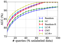
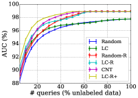
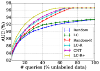
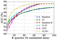
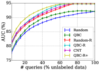
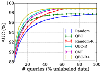
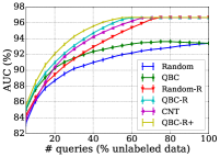
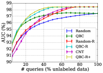
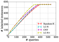
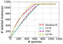
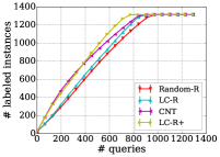
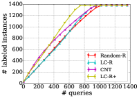
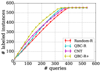
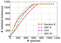
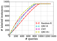
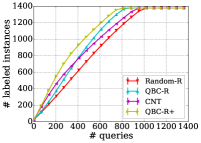
Figure 2 shows the AUC results of different query strategies. For each case, we present the average values and 95% C.I. of repeated 300 trials with different train/test splits. In addition, Figure 3 compares the relations between the number of queries and the number of labeled instances across different query strategies. Note that in the relational active learning setting querying a single unlabeled instance will result in one or more labeled instances. According to Figure 2 and Figure 3, we have the following observations:

First, by comparing query strategies under the settings (ii) and (iii) with setting (i), we observe that incorporating relational reasoning into active learning substantially improves the AUC performance of each query strategy. In addition, we find the query order, which is supposed to be different for each strategy, does not affect $\mathcal{D}_{l}$ at the end when $\mathcal{D}\subseteq\mathcal{D}_{l}$. Thus, it partly verifies Corollary 1.1. Second, our proposed LC-R+ and QBC-R+ significantly outperform other compared query strategies. Specifically, when comparing them with LC-R and QBC-R, we see that incorporating relational reasoning into directing the queries helps to train a better classifier. Figure 3 shows that LC-R+ and QBC-R+ lead to more labeled instances when using the same amount of queries than that of LC-R and QBC-R. This partly contributes to the performance gain. Third, LC-R+ and QBC-R+ are more effective at both collecting a larger labeled set and training better classifiers than the CNT baseline. In addition, by comparing CNT with LC-R, QBC-R, and Random-R, we observe that a larger size of the labeled set does not always lead to a better performance. Such observations demonstrate the necessity of combining deterministic relational reasoning and probabilistic machine learning in designing query strategies.

(a) Data Mining - LC

(b) Geometry - LC

(c) Physics - LC

(d) Precalculus - LC

(e) Data Mining - QBC

(f) Geometry -QBC

(g) Physics - QBC

(h) Precalculus - QBC

Figure 2: Comparison of different query strategies’ AUC scores for concept prerequisite learning.

(a) Data Mining - LC

(b) Geometry - LC

(c) Physics - LC

(d) Precalculus - LC

(e) Data Mining - QBC

(f) Geometry - QBC

(g) Physics - QBC

(h) Precalculus - QBC

Figure 3: Comparison of relations between the number of queries and the number of labeled instances when using different query strategies.

(a) Data Mining

(b) Geometry

(c) Physics

(d) Precalculus

Figure 4: The average runtime for calculating the new closure using Theorem 1 v.s. the size of current labeled closure $|H|$.

5.4.2 Efficiency Study

The proposed reasoning module is designed to be plugged into any algorithm that needs reasoning of strict orders. Thus besides verifying effectiveness, it is also important to investigate its efficiency. We conduct empirical studies on the runtime of the reasoning module.

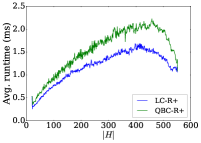
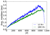
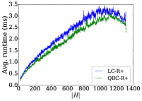
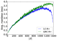
Figure 4 shows the relation between the average runtime for calculating the new closure using Theorem 1 and the size of the current labeled closure $|H|$. Results for both LBC-R+ and QBC-R+ are presented. We can see that as $|H|$ keeps increasing during the pool-based active learning process, the average runtime of calculating $C_{(x,y)}$ increases almost linearly and even decreases a little at the end. Although the worst case time complexity for calculating Theorem 1 is $O(|H|^{3})$ (for $O_{(a,b)}$) and $O(|H|^{2})$ (for others), the runtime required is directly related to the number of ascendants and descendants of elements in $V$, which is usually different for the four strict order datasets used. If the few ascendants and descendants effectively control the size of calculations as we have observed, the runtime will be short regardless of a large $|H|$. This might explain why the growth of calculating $C_{(x,y)}$ is near linear. We also empirically evaluate the effects of using Prop. 4 on the efficiency and include the results in the supplemental material.

6 Conclusion

We propose an active learning framework tailored to relational data in the form of strict partial orders. An efficient reasoning module is proposed to extend two commonly used query strategies – uncertainty sampling and query by committee. Experiments on concept prerequisite learning show that incorporating relational reasoning in both selecting valuable examples to label and expanding the training set significantly improves standard active learning approaches. Future work could be to explore the following: (i) apply the reasoning module to extend other query strategies; (ii) active learning of strict partial orders from a noisy oracle.

Appendix A Supplemental Material

A.1 Proof of Proposition 1

Proof.

For any two supersets $H_{1}\neq H_{2}$ of $H$ whose oracles $W_{H_{1}},W_{H_{2}}$ are complete, $W_{H_{1}\cap H_{2}}$, on a smaller set $H_{1}\cap H_{2}$, is also complete (by definition). ∎

A.2 Proof of Proposition 2

Proof.

For any $(a,b),(b,c)\in H\cap G$, because $W_{H}$ is complete, $(a,c)\in H\cap G$ (by Definition 4 (i)). For any $(a,b)\in H\cap G$, $(b,c)\in H\cap G^{c}\subseteq(H\cap G)^{c}$ (by Definition 4 (iv)). Therefore, $H\cap G$ is also a strict order of $V$ (by Definition 1). ∎

A.3 Proof of Theorem 1

A.3.1 Well-definiteness

It is trivial that if $W_{H}$ is complete, $G\cap(H\cup N_{(x,y)})$ is also a strict order. Therefore, $N^{\prime\prime}_{(c,d)}$ is well defined, so is $O_{(x,y)}$.

A.3.2 Necessity

One can easily verify that if $(x,y)\in G\cap H^{c}$, both $N_{(x,y)}\subseteq\overline{H^{\prime}}$ (Definition 3 (i)), $R_{(x,y)}\subseteq\overline{H^{\prime}}$ (Definition 3 (iv)), and $S_{(x,y)}\cup T_{(x,y)}\cup O_{(x,y)}\subseteq\overline{H^{\prime}}$ (Definition 3 (ii),(iii)) from the definition of closure, and likewise if $(x,y)\not\in G$, $N^{\prime}_{(x,y)}\subseteq\overline{H^{\prime}}$ (Definition 3 (ii), (iii)). In another word, $C_{(x,y)}(H)\subseteq\overline{H^{\prime}}$. Also, see Fig. 1 for the explanation of each necessary condition mentioned.

A.3.3 Sufficiency

One can see $A_{a^{\prime}}^{G}\subseteq A_{a}^{G}$ if $a^{\prime}\in A_{a}^{G}$ and $D_{a^{\prime}}^{G}\subseteq D_{a}^{G}$ if $a^{\prime}\in D_{a}^{G}$. That is, an ancestor of ancestor is also an ancestor (briefly, AAA), and a descendant of descendant is also a descendant (briefly, DDD).

Now we proceed to prove $C_{(x,y)}$ is complete using contradiction which finalizes the proof of our result $C_{(x,y)}=\overline{H^{\prime}}$. If $C_{(x,y)}$ is not complete, by definition, one of the four conditions in Definition 3 must fail.

If Definition 3 (i) fails, there must exist $a,b,c$ such that $(a,b)\in C_{(x,y)}\cap G$, $(b,c)\in C_{(x,y)}\cap G$, while $(a,c)\not\in C_{(x,y)}$. In this case, if both $(a,b)$ and $(b,c)$ are from $H$, because $H$ is complete, $(a,c)\in H\cap G$ contradicts the assumption. Hence at least one of $(a,b)$ and $(b,c)$ is not included in $H$. By the definition of $C_{(x,y)}$, if one pair belongs to $G\cap H^{c}$, it must come from $N_{(x,y)}$. Therefore, it implies $(x,y)\in G\cap H^{c}$.

Cases 1: If $(a,b)\in N_{(x,y)}$ and $(b,c)\in N_{(x,y)}$, $(y,b)\in G$ and $(b,x)\in G$. That however implies $(y,x)\in G$, contradicting $G$’s definition as a strict order (See Definition 1 (ii)).

Cases 2: If $(a,b)\in N_{(x,y)}$ and $(b,c)\in H$, $a\in A_{x}^{G\cap H}$ and $c\in D_{y}^{G\cap H}$ (by DDD). It implies $(a,c)\in N_{(x,y)}\subseteq C_{(x,y)}$.

Cases 3: If $(a,b)\in H$ and $(b,c)\in N_{(x,y)}$, $a\in A_{x}^{G\cap H}$ (by AAA) and $c\in D_{y}^{G\cap H}$. It implies $(a,c)\in N_{(x,y)}\subseteq C_{(x,y)}$.

In summary, Definition 3 (i) holds for $C_{(x,y)}$.

If Definition 3 (ii) fails, there must exist $a,b,c$ such that $(a,b)\in C_{(x,y)}\cap G=G\cap(H\cup N_{(x,y)})$, $(a,c)\in C_{(x,y)}\cap G^{c}$, while $(b,c)\not\in C_{(x,y)}$. In this case, if both $(a,b)$ and $(a,c)$ are from $H$, because $H$ is complete, $(b,c)\in H\cap G^{c}$ contradicts the assumption. Hence at least one of $(a,b)$ and $(a,c)$ is not included in $H$. We divide the statement into the following cases to discuss:

Cases 1: If $(x,y)\in G$, $(a,b)\in N_{(x,y)}$, and $(a,c)\in H\cap G^{c}$, $(a,x)\in{G\cap H}$ and $(y,b)\in{G\cap H}$. Because $(a,x)\in{H\cap G}$, and $(a,c)\in H\cap G^{c}$, $(x,c)\in H\cap G^{c}$. Because $\{(x,y),(y,b)\}\subseteq G\cap(H\cup N_{(x,y)})$, $(x,b)\in G\cap(H\cup N_{(x,y)})$. Therefore, $(b,c)\in N^{\prime\prime}_{(x,c)}\subseteq C_{(x,y)}$.

Cases 2: If $(x,y)\in G$ and $(a,c)\in R_{(x,y)}$, $(c,a)\in N_{(x,y)}$, thus $(c,b)\in N_{(x,y)}$. It implies $(b,c)\in R_{(x,y)}\subseteq C_{(x,y)}$.

Cases 3: If $(x,y)\in G$ and $(a,c)\in S_{(x,y)}$, $(y,a)\in G\cap H$ and $\exists(d,c)\in G^{c}\cap H$ such that $(d,x)\in G\cap H$. Thus, $(x,c)\in G^{c}\cap H\Rightarrow(y,c)\in S_{(x,y)}\Rightarrow(b,c)\in N^{\prime\prime}_{(y,c)}\subseteq C_{(x,y)}$.

Cases 4: If $(x,y)\in G$ and $(a,c)\in T_{(x,y)}$, $(c,x)\in G\cap H$ and $\exists(a,d)\in G^{c}\cap H$ such that $(y,d)\in G\cap H$. Thus, $(a,y)\in G^{c}\cap H\Rightarrow(a,x)\in T_{(x,y)}\Rightarrow(a,b)\not\in N_{(x,y)}$. Because $(a,b)\in G\cap(H\cup N_{(x,y)})$, one has $(a,b)\in G\cap H\Rightarrow(b,x)\in T_{(x,y)}\Rightarrow(b,c)\in N^{\prime\prime}_{(b,x)}\subseteq C_{(x,y)}$.

Cases 5: If $(x,y)\in G$ and $(a,c)\in O_{(x,y)}$, there exists $(d,e)\in S_{(a,b)}\cup T_{(a,b)}$ such that $(a,c)\in N^{\prime\prime}_{(d,e)}$. Therefore, $\{(a,b),(d,a),(c,e)\}\subseteq G\cap(H\cup N_{(x,y)})$. Hence, $(b,c)\in N^{\prime\prime}_{(d,e)}\subseteq C_{(x,y)}$.

Cases 6: If $(x,y)\in G^{c}$, we have $(a,b)\in G\cap H$ and $(a,c)\in N^{\prime}_{(x,y)}$. Thus $(x,b)\in G\cap H\Rightarrow(b,c)\in N^{\prime}_{(x,y)}\subseteq C_{(x,y)}$.

In summary, all six cases above contradict the assumption $(b,c)\not\in C_{(x,y)}$. Thus Definition 3 (ii) holds for $C_{(x,y)}$. Given we have verified the condition of Definition 3 (ii), one can also prove that Definition 3 (iii) holds in a similar way, because their statements as well as definitions of $S_{(x,y)}$ and $T_{(x,y)}$ are symmetric.

One can easily see that Definition 3 (iv) holds for $C_{(x,y)}$, because $G\cap(H\cup N_{(x,y)})$ is also a strict order and $R_{(x,y)}\subseteq C_{(x,y)}$. $\square$

A.4 Proof of Proposition 3

Proof.

If $(c,d)\in S_{(a,b)}$, $c\in D_{b}^{G\cap H}\cup\{b\}$. then $c\not\in A_{a}^{G\cap H}\cup\{a\}$, thus $D_{c}^{G\cap(H\cup N_{(a,b)})}=D_{c}^{G\cap H}$ (by Definition of $N_{(a,b)}$). It holds that $D_{c}^{G\cap(H\cup N_{(a,b)})}\cup\{c\}\subseteq D_{b}^{G\cap H}\cup\{b\}$. Therefore, one has $N^{\prime\prime}_{(c,d)}\subseteq N^{\prime\prime}_{(b,d)}\subseteq O_{(a,b)}$ if $(c,d)\in S_{(a,b)}$. Likewise, $N^{\prime\prime}_{(c,d)}\subseteq N^{\prime\prime}_{(c,a)}\subseteq O_{(a,b)}$ if $(c,d)\in T_{(a,b)}$. One has

$$O_{(a,b)}=\left[\bigcup_{(c,d)\in S_{(a,b)}}N^{\prime\prime}_{(b,d)}\right]\cup\left[\bigcup_{(c,d)\in T_{(a,b)}}N^{\prime\prime}_{(c,a)}\right],$$

whose time complexity is $O(|H|^{3})$. ∎

A.5 Proof of Proposition 4

Proof.

Let $(c^{\prime},d^{\prime})\in N^{\prime\prime}_{(c,d)}$. If $d^{\prime}\neq d$, $(d^{\prime},d)\in G\cap(H\cup N_{(a,b)})$. Then, $A_{d^{\prime}}^{G\cap(H\cup N_{(a,b)})}\subseteq A_{d}^{G\cap(H\cup N_{(a,b)})}$ (AAA). Thus,

$$A_{d^{\prime}}^{G\cap(H\cup N_{(a,b)})}\cup\{d^{\prime}\}\subseteq A_{d}^{G\cap(H\cup N_{(a,b)})}\cup\{d\}.$$

Likewise,

$$D_{c^{\prime}}^{G\cap(H\cup N_{(a,b)})}\cup\{c^{\prime}\}\in D_{c}^{G\cap(H\cup N_{(a,b)})}\cup\{c\}.$$

By the definition of $N^{\prime\prime}_{(c^{\prime},d^{\prime})}$ and $N^{\prime\prime}_{(c,d)}$, one has $N^{\prime\prime}_{(c^{\prime},d^{\prime})}\subseteq N^{\prime\prime}_{(c,d)}$. ∎

A.6 Proof of Theorem 2

We first introduce the notion of transitive reduction before we proceed:

Definition 6 (Transitive Reduction Aho et al. (1972)).

Let G be a directed acyclic graph. We say G is a transitive reduction of G if:

1. There is a directed path from vertex u to vertex v in G iff there is a directed path from u to v in G, and

2. There is no graph with fewer arcs than G satisfying (i).

For directed acyclic graph $G$, Aho et al. (1972) have shown that the transitive reduction is unique and is a subgraph of $G$. Let $G$ be a simple directed acyclic graph (DAG). In compliance with Def. 4, we use $\overline{G}$ to denote the transitive closure of $G$. Define $S(G)$ as the set of graphs such that every graph in $S(G)$ has the same transitive closure as $G$, i.e.,

$$S(G)\coloneqq\{G^{\prime}\mid\overline{G^{\prime}}=\overline{G}\}$$

Aho et al. (1972) have shown that $S(G)$ is closed under intersection and union. Further more, for DAG $G$, the following relationship holds:

$$\underline{G}=\bigcap_{G^{\prime}\in S(G)}G^{\prime}\subseteq G\subseteq\bigcup_{G^{\prime}\in S(G)}G^{\prime}=\overline{G}$$

Next, we give the proof of Theorem 2 below.

Proof.

With the fact that negative labels from the query oracle cannot help to induce positive labels in the graph, we can bound the number of queries, $m$, needed to learn a classifier:

$$m\geq|\underline{G}|$$

The proof is by simple contradiction based on the definition of the transitive reduction of $G$ and the fact that $A$ is a consistent learner. On the other hand, there is a learning algorithm $A$ that simply remembers all the queries with positive labels and predict all the other inputs as negative. For this algorithm $A$, it suffices for $A$ to make $|\overline{G}|$ queries. ∎

A.7 Experiment Environment

All experiments are conducted on an Ubuntu 14.04 server with 256GB RAM and 32 Intel Xeon E5-2630 v3 @ 2.40GHz processors. Active learning query strategies are implemented in Python2.7. Code and data will be publicly available.

A.8 Effectiveness of Proposition 4

Domain	LC-R+		QBC-R+
	w/o pruning	w/ pruning	w/o pruning	w/ pruning
Data mining	5.5	3.3 (-40%)	5.5	2.6 (-53%)
Geometry	85.5	39.2 (-54%)	69.6	31.4 (-55%)
Physics	111.0	58.8 (-47%)	117.1	60.2 (-49%)
Precalculus	134.3	59.9 (-55%)	167.4	74.8 (-55%)

Table 4: The effect of Proposition 4 on the total runtime (s) of $O_{(a,b)}$ calculation in Theorem 1 for a full round of active learning (until $\mathcal{D}_{u}=\emptyset$).

We also empirically evaluate the effects of using Proposition 4 on the efficiency. Specifically, we measure the total runtime of $O_{(a,b)}$ calculation in Theorem 1 for a full round of active learning (until $\mathcal{D}_{u}=\emptyset$) with and without applying the pruning rule induced by Proposition 4. The results are shown in Table 4 where the numbers are the average runtime over all 300 different rounds of active learning for each dataset. We can see that the pruning can lead to a speedup of 40-55% in the LC-R+ experiments and a speedup of 49-55% in the QBC-R+ experiments, which shows that Proposition 4 is helpful for higher efficiency.

References

- Aho et al. (1972) Alfred V. Aho, Michael R Garey, and Jeffrey D. Ullman. 1972. The transitive reduction of a directed graph. SIAM Journal on Computing 1(2):131–137.
- Angluin (1988) Dana Angluin. 1988. Queries and concept learning. Machine learning 2(4):319–342.
- Blei et al. (2003) David M Blei, Andrew Y Ng, and Michael I Jordan. 2003. Latent Dirichlet allocation. Journal of machine Learning research 3(Jan):993–1022.
- Breiman (2001) Leo Breiman. 2001. Random forests. Machine learning 45(1):5–32.
- Burges et al. (2005) Chris Burges, Tal Shaked, Erin Renshaw, Ari Lazier, Matt Deeds, Nicole Hamilton, and Greg Hullender. 2005. Learning to rank using gradient descent. In Proc. ICML. ACM, pages 89–96.
- Cohn et al. (1996) David A Cohn, Zoubin Ghahramani, and Michael I Jordan. 1996. Active learning with statistical models. Journal of Artificial Intelligence Research 4(1):129–145.
- Donmez and Carbonell (2008) Pinar Donmez and Jaime G Carbonell. 2008. Optimizing estimated loss reduction for active sampling in rank learning. In Proc. ICML. ACM, pages 248–255.
- Getoor and Taskar (2007) Lise Getoor and Ben Taskar. 2007. Introduction to statistical relational learning .
- Gordon et al. (2016) Jonathan Gordon, Linhong Zhu, Aram Galstyan, Prem Natarajan, and Gully Burns. 2016. Modeling concept dependencies in a scientific corpus. In Proc. ACL.
- Kleinberg (1999) Jon M Kleinberg. 1999. Authoritative sources in a hyperlinked environment. Journal of the ACM 46(5):604–632.
- Lewis and Catlett (1994) David D Lewis and Jason Catlett. 1994. Heterogeneous uncertainty sampling for supervised learning. In Proc. ICML. pages 148–156.
- Lewis and Gale (1994) David D Lewis and William A Gale. 1994. A sequential algorithm for training text classifiers. In Proc. SIGIR. pages 3–12.
- Liang et al. (2015) Chen Liang, Zhaohui Wu, Wenyi Huang, and C. Lee Giles. 2015. Measuring prerequisite relations among concepts. In Proc. EMNLP. pages 1668–1674.
- Liang et al. (2018) Chen Liang, Jianbo Ye, Shuting Wang, Bart Pursel, and C Lee Giles. 2018. Investigating active learning for concept prerequisite learning. In Proc. EAAI.
- Liu et al. (2016) Hanxiao Liu, Wanli Ma, Yiming Yang, and Jaime Carbonell. 2016. Learning concept graphs from online educational data. Journal of Artificial Intelligence Research 55:1059–1090.
- Liu (2009) Tie-Yan Liu. 2009. Learning to rank for information retrieval. Foundations and Trends® in Information Retrieval 3(3):225–331.
- Long et al. (2010) Bo Long, Olivier Chapelle, Ya Zhang, Yi Chang, Zhaohui Zheng, and Belle Tseng. 2010. Active learning for ranking through expected loss optimization. In Proc. SIGIR. ACM, pages 267–274.
- Mamitsuka (1998) Naoki Abe Hiroshi Mamitsuka. 1998. Query learning strategies using boosting and bagging. In Proc. ICML. Morgan Kaufmann Pub, volume 1.
- Mikolov et al. (2013) Tomas Mikolov, Ilya Sutskever, Kai Chen, Greg S Corrado, and Jeff Dean. 2013. Distributed representations of words and phrases and their compositionality. In Proc. NIPS. pages 3111–3119.
- Pan et al. (2017) Liangming Pan, Chengjiang Li, Juanzi Li, and Jie Tang. 2017. Prerequisite relation learning for concepts in moocs. In Proc. ACL. ACL, pages 1447–1456.
- Ratinov et al. (2011) Lev Ratinov, Dan Roth, Doug Downey, and Mike Anderson. 2011. Local and global algorithms for disambiguation to Wikipedia. In Proc. ACL. ACL, pages 1375–1384.
- Rendle and Schmidt-Thieme (2008) Steffen Rendle and Lars Schmidt-Thieme. 2008. Active learning of equivalence relations by minimizing the expected loss using constraint inference. In Proc. ICDM. IEEE, pages 1001–1006.
- Scheines et al. (2014) Richard Scheines, Elizabeth Silver, and Ilya Goldin. 2014. Discovering prerequisite relationships among knowledge components. In Proc. EDM. pages 355–356.
- Settles (2010) Burr Settles. 2010. Active learning literature survey. University of Wisconsin, Madison 52(55-66):11.
- Seung et al. (1992) H Sebastian Seung, Manfred Opper, and Haim Sompolinsky. 1992. Query by committee. In Proc. COLT. ACM, pages 287–294.
- Talukdar and Cohen (2012) Partha Pratim Talukdar and William W Cohen. 2012. Crowdsourced comprehension: predicting prerequisite structure in Wikipedia. In Proceedings of the Seventh Workshop on Building Educational Applications Using NLP. ACL, pages 307–315.
- Vuong et al. (2011) Annalies Vuong, Tristan Nixon, and Brendon Towle. 2011. A method for finding prerequisites within a curriculum. In Proc. EDM. pages 211–216.
- Wang et al. (2016) Shuting Wang, Alexander Ororbia, Zhaohui Wu, Kyle Williams, Chen Liang, Bart Pursel, and C. Lee Giles. 2016. Using prerequisites to extract concept maps from textbooks. In Proc. CIKM. ACM, pages 317–326.
- Witten and Milne (2008) Ian Witten and David Milne. 2008. An effective, low-cost measure of semantic relatedness obtained from Wikipedia links. In Proceeding of AAAI Workshop on Wikipedia and Artificial Intelligence: an Evolving Synergy. pages 25–30.