Any modification of the Born rule leads to a violation of the purification and local tomography principles
Abstract
Using the existing classification of all alternatives to the measurement postulates of quantum theory we study the properties of bi-partite systems in these alternative theories. We prove that in all these theories the purification principle is violated, meaning that some mixed states are not the reduction of a pure state in a larger system. This allows us to derive the measurement postulates of quantum theory from the structure of pure states and reversible dynamics, and the requirement that the purification principle holds. The violation of the purification principle implies that there is some irreducible classicality in these theories, which appears like an important clue for the problem of deriving the Born rule within the many-worlds interpretation. We also prove that in all such modifications the task of state tomography with local measurements is impossible, and present a simple toy theory displaying all these exotic non-quantum phenomena. This toy model shows that, contrarily to previous claims, it is possible to modify the Born rule without violating the no-signalling principle. Finally, we argue that the quantum measurement postulates are the most non-classical amongst all alternatives.
1 Introduction
The postulates of quantum theory describe the evolution of physical systems by distinguishing between the cases where observation happens or not. However, these postulates do not specify what constitutes observation, and it seems that an act of observation by one agent can be described as unperturbed dynamics by another Everett (1957). This opens the possibility of deriving the physics of observation within the picture of an agent-free universe that evolves unitarily. This problem has been studied within the dynamical description of quantum measurements Allahverdyan et al. (2013), the decoherence program Zurek (2005) and the Many-Worlds Interpretation of quantum theory Deutsch (1999); Wallace (2010).
In this work, instead of presenting another derivation of the measurement postulates, we take a more neutral approach and analyze all consistent alternatives to the measurement postulates. In particular, we prove that in each such alternative there are mixed states which are not the reduction of a pure state on a larger system. This property singles out the (standard) quantum measurement postulates including the Born Rule.
In our previous work Galley and Masanes (2017) we constructed a complete classification of all alternative measurement postulates, by establishing a correspondence between these and certain representations of the unitary group. However, this classification did not involve the consistency constraints that arise from the compositional structure of the theory; which governs how systems combine to form multi-partite systems. In this work we take into account compositional structure, and prove that all alternative measurement postulates violate two compositional principles: purification Chiribella et al. (2010, 2011) and local tomography Hardy (2001); Barrett (2007). We also present a simple alternative measurement postulate (a toy theory) which illustrates these exotic phenomena. Additionally, this toy theory provides an interesting response to the claims that the Born rule is the only probability assignment consistent with no-signalling Aaronson (2004); Bao et al. (2016); Han and Choi (2016).
In Section 2 we introduce a theory-independent formalism, which allows to study all alternatives to the measurement postulates. We also review the results of our previous work Galley and Masanes (2017). In Section 3 we define the purification and local tomography principles, and show that these are violated by all alternative measurement postulates. In Section 4 we describe a particular and very simple alternative measurement postulate, which illustrates our general results. In Section 5 we discuss our results in the light of existing work. All proofs are in the appendices.
2 Dynamically-quantum theories
In this work we consider all theories that have the same pure states, dynamics and system-composition rule as quantum theory, but have a different structure of measurements and a different rule for assigning probabilities.
2.1 States, transformations and composition postulates
The family of theories under consideration satisfy the following postulates, taken from the standard formulation of quantum theory.
Postulate (Quantum States).
Every finite-dimensional Hilbert space corresponds to a type of system with pure states being the rays of .
Postulate (Quantum Transformations).
The reversible transformations on the pure states are for all .
Postulate (Quantum Composition).
The joint pure states of systems and are the rays of .
2.2 Measurement postulates
Before presenting the generalized measurement postulate we need to introduce the notion of outcome probability function, or OPF. For each measurement outcome of system there is a function that assigns to each ray in the probability for the occurrence of outcome . Any such function is called an OPF. Each system has a (trivial) measurement with only one outcome, which must have probability one for all states. The uniqueness of this trivial measurement is the Causality Axiom of Chiribella et al. (2010). The OPF associated to this outcome is called the unit OPF , satisfying for all . A -outcome measurement is a list of OPFs satisfying the normalization condition . It is not necessarily the case that every list of OPFs satisfying this condition defines a measurement, though this assumption can be made. As an example, the OPFs of quantum theory are the functions
| (1) |
for all Hermitian matrices satisfying . This implies that . (Here and in the rest of the paper we assume that kets are normalized.)
Postulate (Alternative Measurements).
Every type of system has a set of OPFs with a bilinear associative product satisfying the following consistency constraints:
-
C1.
For every and there is an such that for all . That is, the composition of a unitary and a measurement can be globally considered a measurement.
-
C2.
For any pair of different rays in there is an such that . That is, different pure states must be operationally distinguishable.
-
C3.
The -product satisfies and
(2) for all , , , . That is, tensor-product states contain no correlations.
-
C4.
For each and there is an ensemble in such that
(3) for all . That is, the reduced state on conditioned on outcome on (and re-normalized) is a valid mixed state of . In the next sub-section we fully articulate the notions of ensemble and mixed state.
-
C5.
Consider measurements on system with the help of an ancilla . For any ancillary state and any OPF in the composite there exists an OPF on the system such that
(4) for all .
The derivation of these consistency constraints from operational principles is provided in Appendix A. Continuing with the example of quantum theory (1), the -product in this case is
| (5) |
A trivial modification of the Measurement Postulate consists of taking that of quantum mechanics (1) and restricting the set of OPFs in some way, such that not all POVM elements are allowed. In this work, when we refer to “all alternative measurement postulates” we do not include these trivial modifications.
2.3 Mixed states and the Finiteness Principle
A source of systems that prepares state with probability is said to prepare the ensemble . Two ensembles and are equivalent if they are indistinguishable
| (6) |
for all measurements . Note that distinguishability is relative to the postulated set of OPFs . A mixed state is an equivalence class of indistinguishable ensembles, and hence, the structure of mixed states is also relative to . To evaluate an OPF on a mixed state we can take any ensemble of the equivalence class and compute
| (7) |
In general, ensembles can have infinitely-many terms, hence, the number of parameters that are needed to characterize a mixed state can be infinite too. When this is the case, state estimation without additional assumptions is impossible, and for this reason we make the following assumption.
Principle (Finiteness).
Each mixed state of a finite-dimensional system can be characterized by a finite number of parameters.
Recall that in quantum theory we have . And in general, the distinguishability of all rays in implies . These parameters can be chosen to be a fix set of “fiducial” OPFs , which can be used to represent any mixed state as
| (8) |
The fact that OPFs are probabilities implies that any OPF is a linear function of the fiducial OPFs
| (9) |
In other words, the fiducial OPFs constitute a basis of the real vector space spanned by . Using the consistency constraint C1, we define the action
| (10) |
on the vector space spanned by . This associates to system a -dimensional representation of the group . This, together with the other consistency constraints, implies that only certain values of are allowed. For example
2.4 Measurement postulates for single systems
In this subsection we review some of the results obtained in Galley and Masanes (2017). These provide the complete classification of all sets satisfying the Finiteness Principle and the consistency constraints C1 and C2. These results ignore the existence of the -product, C3, C4 and C5. Hence, in alternative measurement postulates with a consistent compositional structure there will be additional restrictions on the valid sets . This is studied in Section 3.
Theorem (Characterization).
If satisfies the Finiteness Principle and C1 then there is a positive integer and a map from to the set of Hermitian matrices such that
| (11) |
for all normalized vectors .
Note that there are many different sets with the same . In particular, since the action
| (12) |
is reducible, the Hermitian matrices can have support on the different irreducible sub-representations of (12), generating sets with very different physical properties. All these possibilities are analyzed in Galley and Masanes (2017).
Theorem (Faithfulness).
If satisfies the Finiteness Principle, C1 and C2, then
- case
-
there is a non-constant .
- case
-
there is such that has support on a sub-representation of the action (12) with odd angular momentum.
3 Features of all alternative measurement postulates
In this section we analyze the compositional structure of alternative measurement postulates. We do so by considering two well known physical principles which, together with other assumptions, have been used to reconstruct the full formalism of quantum theory Masanes and Muller (2011); Chiribella et al. (2011); Dakic and Brukner (2011); Barnum and Wilce (2014). Remarkably, these principles are violated by all alternative measurement postulates.
3.1 The Purification Principle
This principle establishes that any mixed state is the reduction of a pure state in a larger system. This legitimises the “Church of the Larger Hilbert Space”, an approach to physics that always assumes a global pure state when an environment is added to the systems under consideration Nielsen and Chuang (2011).
Principle (Purification).
For each ensemble in there exists a pure state in for some satisfying
| (13) |
for all .
Note that the original version of the purification principle introduced in Chiribella et al. (2010) additionally demands that the purification state is unique up to a unitary transformation on . Also note that the following theorem does not require the Finiteness Principle.
Theorem (No Purification).
All alternative measurements postulates satisfying C1, C2, C3 and C4 violate the purification principle.
This implies that in all alternative measurement postulates there are operational processes, such as mixing two states, which cannot be understood as a reversible transformation on a larger system. In such alternative theories, agents that perform physical operations cannot be integrated in an agent-free universe, as can be done in quantum theory, and the Church of the Larger Hilbert Space is illegitimate. The assumption that agents’ actions can be understood as reversible transformations on a larger system is also the starting point of the many-worlds interpretation of quantum theory. Hence, it seems like the no-purification theorem provides important clues for the derivation of the Born Rule within the many-worlds interpretation Everett (1957); Zurek (2005); Wallace (2010); Deutsch (1999). In section 5.1 we discuss further the possibility of using this result to derive the quantum measurement postulates, and contrast it to Zurek’s envariance based derivation of the Born rule.
3.2 The Local Tomography Principle
This principle has been widely used in reconstructions of quantum theory and the formulation of alternative toy theories Dakic and Brukner (2011); Masanes and Muller (2011); Chiribella et al. (2011); Barnum and Wilce (2014); Masanes et al. (2013); Höhn (2017). One of the reasons is that it endows the set of mixed states with a tensor-product structure Barrett (2007). This principle states that any bi-partite state is characterized by the correlations between local measurements. That is, two different mixed states on must provide different outcome probabilities
| (14) |
for some local measurements , . Using the notation introduced in (9) we can formulate this principle as follows.
Principle (Local Tomography).
If is a basis of and is a basis of then is a basis of , where and .
A theory is said to violate local tomography if at least one composite system within the theory violates local tomography. Therefore, it is sufficient to analyze the particular bi-partite system .
Theorem (No Local Tomography).
All alternative measurements and satisfying C1, C2, C3 and the Finiteness Principle violate the local tomography principle.
The above result is proven in Appendix E. We first show that all transitive theories which obey the local tomography principle have a group action acting on the mixed states which has a certain structure. Any group action of the form (10) which does not have this structure must correspond to a system which violates local tomography. We show that all representations of which correspond to systems with alternative measurement postulates do not have this structure. This entails that all non-quantum systems which are composites of two systems violate local tomography.
The technical result proven to show this is the following. All non-quantum irreducible representations of which are sub-representations of the action (12) have a sub-representation when restricted to the subgroup . Here denotes the trivial representation of .
3.2.1 Comment on systems
In quantum theory any () system can be simulated using some number of qubits. In this sense qubits can be viewed as fundemental information units Masanes et al. (2013). Since systems have a priveleged status it is natural to ask whether systems in theories with modified measurement postulates are locally tomographic. The proof technique used for the No Local Tomography Theorem applies only to a certain family of these systems. However all instances of systems studied by the authors which were not part of this family were found to not be locally tomographic. We conjecture that all violate the local tomography principle.
4 A Toy Theory
In this section we present a simple alternative measurement postulate which serves as example for the results that we have proven in general (violation of the purification and local tomography Principles). In Appendix G it is proven that this alternative measurement postulate satisfies all consistency constraints (C1, C2, C3, C4, C5) except for the associativity of the -product. This implies that this toy theory is only fully consistent when dealing with single and bi-partite systems. However, most of the work in the field of general probabilistic theories (GPTs) focuses on bi-partite systems, because these already display very rich phenomenology. In the following we consider two local subsystems of dimension and with sets of OPFs and . The composite (global) system has a set of OPFs .
Definition (Local effects ).
Let be the projector onto the symmetric subspace of . To each Hermitian matrix satisfying
-
•
,
-
•
for some and ,
-
•
for some and ,
there corresponds the OPF
| (15) |
The unit OPF corresponds to .
That is, both matrices, and , have to be not-necessarily-normalized mixtures of symmetric product states.
Example (Canonical measurement for prime).
For the case where is prime there exists a canonical measurement which can be constructed as follows. Consider the mutually unbiased bases (MUBs): where runs from to Bandyopadhyay et al. (2001). Then we can associate an OPF to each Hermitian matrix . Since the basis elements of these MUBs form a complex projective 2-design Klappenecker and Roetteler (2005), by the definition of 2-design Zhu et al. (2016), we have the normalization constraint:
| (16) |
and hence the set of OPFs forms a measurement.
Definition ( product).
For any pair of OPFs and the Hermitian matrix corresponding to their product is
| (17) |
where and are the projectors onto the symmetric and anti-symmetric subspaces of , and analogously for and .
This product is clearly bilinear and, by using the identity , we can check that .
We observe that not all effects are of the form . Hence the set of effects on the joint system is not , but has to be extended to to include these joint product effects.
Definition (Global effects ).
The set should include all product OPFs , all OPFs of understood as a single system, and their convex combinations.
The identity perfectly shows that the vector space is larger than the tensor product of the vector spaces and , by the extra term . This implies that this toy theory violates the Local-Tomography Principle.
The joint probability of outcomes and on the entangled state can be written as
When we only consider sub-system outcome probabilities are given by
| (18) | |||||
| (19) |
where the reduced state must necessarily be
| (20) |
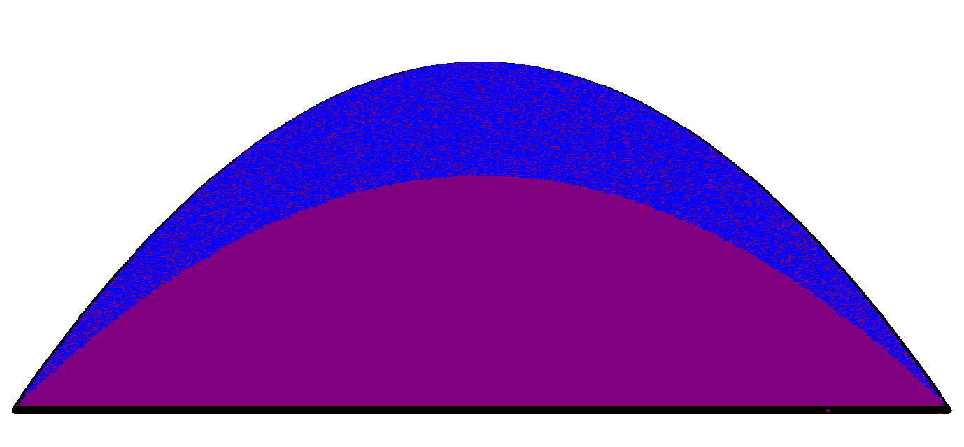
All these reductions of pure bipartite states are contained in the convex hull of , as required by the consistency constraint . However, not all mixtures of can be written as one such reduction (20). That is, the purification postulate is violated. This phenomenon is graphically shown in Figure 1.
5 Discussion
5.1 Interpreting results as a derivation of the Born rule
In this paper we have shown that all modifications to the quantum measurements lead to violations of the purification and local tomography principles. This entails that one can derive the measurement postulates of quantum theory from the structure of pure states and dynamics and either the assumption of local tomography or purification. Such a derivation uses the operational framework which can be viewed as a background assumption.
A derivation of the Born rule which starts from similar assumptions to ours, but not within an operational setting, is the envariance based derivation of Zurek Zurek (2005). Zurek begins by assuming the dynamical structure of quantum theory and the assumption that quantum theory is universal, which is to say that all the phenomena we observe can be explained in terms of quantum systems interacting. Specifically the classical worlds of devices can be modelled quantum mechanically, including the measurement process. We observe that this is philosophically very different to the operational approach adopted in this work, which takes the classical world as a primitive. By assuming the dynamical structure of quantum theory and the assumption of universality (as well as some auxiliary assumptions) Zurek shows that measurements are associated to orthonormal bases, and that outcome probabilities are given by the Born rule. For criticisms of Zurek’s approach we refer the reader to Caves (2004); Schlosshauer and Fine (2005); Barnum (2003); Mohrhoff (2004).
We observe that the purification postulate seems linked to the notion that quantum theory is universal, in the sense that any classical uncertainty can be explained as originating from some pure global quantum state. This shows an interesting link to Zurek’s derivation, since although we work within an operational framework, the concept of purification is linked to the idea that quantum theory is universal. This shows that we can also rely on a concept linked to universality in order to derive the Born rule (and the structure of measurements) within an operational approach.
We observe that we can also derive the measurement postulates of quantum theory from the assumption of local tomography, which does not have this connotation of universality.
5.2 No-signalling
Multiple proofs have been put forward which claim to show that violations of the Born rule lead to signalling Aaronson (2004); Bao et al. (2016); Han and Choi (2016). However the authors only consider modifications of the Born rule of a specific type. In Aaronson (2004); Bao et al. (2016) the authors only consider modifications of the Born rule of the following form:
| (21) |
where . Modifications of this form are very restricted. By modifying all the measurement postulates of quantum theory, we can create toy models like the one introduced, which are non-signalling (as we will show momentarily). This shows that by modifying the Born rule in a more general manner one can avoid issues of signalling.
In the case of the toy model it is immediate to see that it is consistent with no-signalling. The condition of no-signalling is equivalent to the existence of a well defined state-space for the subsystem (i.e. independent of action on the other subsystem). We see then that no-signalling is just a consequence of there existing a well defined reduced state Chiribella et al. (2010).
5.3 Purification as a constraint on physical theories
In Theorem 19 of Chiribella et al. (2010) the authors show that any two convex theories with the same states (pure and mixed) which obey purification are the same theory. In other words “states specify the theory” for theories with purification Chiribella et al. (2010). In this chapter we show that in the case of theories with pure states and dynamical group , any two theories which obey purification with the same pure states and reversible dynamics are the same. This means that for a restricted family of theories (those with systems with pure states and dynamical group ) we have the same result as Theorem 19 of Chiribella et al. (2010) but with different assumptions. It would be interesting to establish whether this is a general feature of theories with purification, namely that the pure states and reversible dynamics specify the theory.
5.4 The quantum measurement postulates are the most non-classical
One consequence of the classification in Galley and Masanes (2017) is that the quantum measurement postulates are the ones which give the lowest dimensional state spaces. In this sense the quantum measurement postulates are the most non-classical, since they give rise to the state spaces with the higest degree of indistinguishable ensemles Mielnik (1974). We remember that in classical probability theory all ensembles are distinguishable.
The violation of purification seems to indicate some other, distinct type of classicality. In theories which violate purification there are some preparations which can only be modelled as arising from a classical mixture of pure states. There appears to be some sort of irreducible classicality. However in theories which obey purification we can always model such preparations as arising from the reduction of a global pure state. Since the quantum measurement postulates are the only ones which give rise to systems which obey purification they can be viewed as the most non-classical amongst all alternatives.
Hence we see that according to these two distinct notions of non-classicality the quantum measurement postulates are the most non-classical amonst all possible measurement postulates.
5.5 Toy model
The toy model can be obtained by restricting the states and measurements of two pairs of quantum systems and . In this sense we obtain a theory which violates both local tomography and purification. This method of constructing theories is similar to real vector space quantum theory, which can also be obtained from a suitable restriction of quantum states and also violates local tomography. The main limitation of the toy model is that it does not straightforwardly extend to more than two systems. There is a natural generalisation of the toy model to consider effects to be linear in for , however showing the consistency of the reduced state spaces and joint effects is more complex.
5.6 Theories which decohere to quantum theory
A recent result Lee and Selby (2018) shows that all operational theories which decohere to quantum theory (in an analogous way to which quantum theory decoheres to classical theory) must violate either purification or causality (or both). The authors define a hyper-decoherence map which maps states of the post-quantum system to states of a quantum system (embedded within the post-quantum system). This map obeys the following properties:
-
1.
Terminality: applying the map followed by the unit effect is equivalent to just applying the unit effect.
-
2.
Idempotency: applying the map twice is the same as applying it once.
-
3.
The pure states of the quantum subsystem are pure states of the post-quantum system. Similarly the maximally mixed state of the quantum subsystem is the maximally mixed state of the post-quantum system.
Now we ask whether the systems in this paper (which violate purification) can correspond to post-quantum systems which decohere to quantum systems in some reasonable manner. We consider the toy model with pure states and no restriction on the allowed effects (this toy model is only valid for single systems). Now consider a linear map from to some embedded quantum system such that the pure states of the system are also of the form (by property 3). This map must be of the form . Hence its action on the state space gives an identical state space and the map is trivial.111We thank referee 1 for this observation. This shows that the only hyper-decoherence maps which obey all the conditions set out by Lee and Selby must be trivial.
As we argue later, it is not immediately obvious that a hyper-decoherence map should obey condition 3. We now define a hyper-decoherence like map which does not meet this condition. Consider the following map where we label the copies of , and :
| (22) | ||||
| (23) |
This meets properties 1 and 2, but not 3. Indeed the states are not valid mixed states of the post-quantum system. The image of this map for all is a quantum state space.
The authors of Lee and Selby (2018) show that requirement 3 can be replaced by the requirement that the hyper-decoherence map maps between systems with the same information dimension. As shown in Galley and Masanes (2017) (for the case ) the information dimension of an unrestricted state space is larger than that of a qubit.
The hyper-decoherence map of Lee and Selby (2018) is inspired by the decoherence map which exists between quantum and classical state spaces. The map introduced in this section is very different from this, since its image is not an embedded state space; however it may be that decoherence between a post-quantum theory and quantum theory is very different from what our quantum/classical intuitions might lead us to believe.
The decoherence map of equation (22) appears strange at first, since it maps states of a post-quantum system to a sub-system which is embedded in such a way that its states are not valid states of the post-quantum system. However the image of this decoherence map is actually the state space one would obtain if one had access to the post-quantum system but only a restricted set of measurements. An observer with access to the post-quantum system but only effects of the form would reconstruct a quantum state space. Hence the link between the system and subsystem becomes clearer: the quantum sub-system is obtained from the post-quantum system by restricting the measurements on the post-quantum system. We emphasise once more that the toy model with unrestricted effects does not compose.
6 Conclusion
6.1 Summary
We have studied composition in general theories which have the same dynamical and compositional postulates as quantum theory but which have different measurement postulates. We presented a toy model of a bi-partite system with alternative measurement rules, showing that composition is possible in such theories. We showed that all such theories violate two compositional principles: local tomography and purification.
6.2 Future work
The toy model introduced in this work applies only to bi-partite systems and is simulable with quantum theory. Hence an important next step is constructing a toy model with alternative measurement rules which is consistent with composition of more than two systems. This requires a product which is associative. This construction may prove impossible, or it may be the case that all valid constructions are simulable by quantum theory. We suggest that there are three possibilities when considering theories with fully associative products.
Possibility 1. (Logical consistency of postulates of Quantum Theory). The only measurement postulates which are fully consistent with the associativity of composition are the quantum measurement postulates.
If this were the case it would show that the postulates of quantum theory are not independent. Only the quantum measurement rules would be consistent with the dynamical and compositional postulates (and operationalism). However it may be the case that we can develop theories with alternative Born rules which compose with an associative product, but that all these theories are simulable by quantum theory.
Possibility 2. (Simulability of systems in theories with alternative postulates). The only measurement postulates which are fully consistent with the dynamical postulates of quantum theory describe systems which are simulable with a finite number of quantum systems.
Possibility 3. (Non-simulability of systems in theories with alternative postulates). There exist measurement postulates which are fully consistent with the dynamical postulates of quantum theory which describe systems which are not simulable with a finite number of quantum systems.
This final possibility would be interesting from the perspective of GPTs as it would show that there are full theories which can be obtained by modifying the measurement postulates of quantum theory. It would show that quantum theory is not, in fact, an island in theory space.
7 Acknowledgements
We are grateful to Jonathan Barrett and Robin Lorenz for helpful discussions. We thank the referees for their comments which helped substantially improve the first version of this manuscript. TG is supported by the Engineering and Physical Sciences Research Council [grant number EP/L015242/1]. LM is funded by EPSRC.
References
- Everett [1957] Hugh Everett. “Relative State” formulation of quantum mechanics. Rev. Mod. Phys., 29:454–462, Jul 1957. doi: 10.1103/RevModPhys.29.454.
- Allahverdyan et al. [2013] A. E. Allahverdyan, R. Balian, and T. M. Nieuwenhuizen. Understanding quantum measurement from the solution of dynamical models. Phys. Rep., 525:1–166, April 2013. doi: 10.1016/j.physrep.2012.11.001.
- Zurek [2005] Wojciech Hubert Zurek. Probabilities from entanglement, Born’s rule from envariance. Phys. Rev. A, 71:052105, May 2005. doi: 10.1103/PhysRevA.71.052105.
- Deutsch [1999] David Deutsch. Quantum theory of probability and decisions. Proceedings of the Royal Society of London A: Mathematical, Physical and Engineering Sciences, 455(1988):3129–3137, 1999. doi: 10.1098/rspa.1999.0443.
- Wallace [2010] David Wallace. How to Prove the Born Rule. In Adrian Kent Simon Saunders, Jon Barrett and David Wallace, editors, Many Worlds? Everett, Quantum Theory, and Reality. Oxford University Press, 2010.
- Galley and Masanes [2017] Thomas D. Galley and Lluis Masanes. Classification of all alternatives to the born rule in terms of informational properties. Quantum, 1:15, jul 2017. doi: 10.22331/q-2017-07-14-15.
- Chiribella et al. [2010] Giulio Chiribella, Giacomo Mauro DAriano, and Paolo Perinotti. Probabilistic theories with purification. Physical Review A, 81(6):062348, jun 2010. doi: 10.1103/PhysRevA.81.062348.
- Chiribella et al. [2011] Giulio Chiribella, Giacomo Mauro DAriano, and Paolo Perinotti. Informational derivation of quantum theory. Physical Review A, 84(1):012311, July 2011. doi: 10.1103/PhysRevA.84.012311.
- Hardy [2001] Lucien Hardy. Quantum theory from five reasonable axioms. eprint arXiv:quant-ph/0101012, January 2001.
- Barrett [2007] Jonathan Barrett. Information processing in generalized probabilistic theories. Phys. Rev. A, 75:032304, March 2007. doi: 10.1103/PhysRevA.75.032304.
- Aaronson [2004] Scott Aaronson. Is Quantum Mechanics An Island In Theoryspace? eprint arXiv:quant-ph/0401062, 2004.
- Bao et al. [2016] Ning Bao, Adam Bouland, and Stephen P. Jordan. Grover search and the no-signaling principle. Physical review letters, 117(12):120501, 2016. URL https://journals.aps.org/prl/abstract/10.1103/PhysRevLett.117.120501.
- Han and Choi [2016] Y. D. Han and T. Choi. Quantum Probability assignment limited by relativistic causality. Sci. Rep., 6:22986, July 2016. doi: 10.1038/srep22986.
- Masanes and Muller [2011] Lluís Masanes and Markus P. Muller. A derivation of quantum theory from physical requirements. New Journal of Physics, 13(6):063001, 2011. doi: 10.1088/1367-2630/13/6/063001.
- Dakic and Brukner [2011] Borivoje Dakic and Caslav Brukner. Quantum Theory and Beyond: Is Entanglement Special? In H. Halvorson, editor, Deep Beauty - Understanding the Quantum World through Mathematical Innovation, pages 365–392. Cambridge University Press, 2011.
- Barnum and Wilce [2014] H. Barnum and A. Wilce. Local Tomography and the Jordan Structure of Quantum Theory. Foundations of Physics, 44:192–212, February 2014. doi: 10.1007/s10701-014-9777-1.
- Nielsen and Chuang [2011] Michael A. Nielsen and Isaac L. Chuang. Quantum Computation and Quantum Information: 10th Anniversary Edition. Cambridge University Press, New York, NY, USA, 10th edition, 2011. ISBN 1107002176, 9781107002173.
- Masanes et al. [2013] Lluis Masanes, Markus P. Muller, Remigiusz Augusiak, and David Perez-Garcia. Existence of an information unit as a postulate of quantum theory. Proceedings of the National Academy of Sciences, 110(41):16373–16377, 2013. doi: 10.1073/pnas.1304884110.
- Höhn [2017] Philipp Andres Höhn. Toolbox for reconstructing quantum theory from rules on information acquisition. Quantum, 1:38, December 2017. ISSN 2521-327X. doi: 10.22331/q-2017-12-14-38.
- Bandyopadhyay et al. [2001] Somshubhro Bandyopadhyay, P. Oscar Boykin, Vwani Roychowdhury, and Farrokh Vatan. A new proof for the existence of mutually unbiased bases. eprint arXiv:quant-ph/0103162, March 2001.
- Klappenecker and Roetteler [2005] Andreas Klappenecker and Martin Roetteler. Mutually Unbiased Bases are Complex Projective 2-Designs. eprint arXiv:quant-ph/0502031, February 2005.
- Zhu et al. [2016] Huangjun Zhu, Richard Kueng, Markus Grassl, and David Gross. The Clifford group fails gracefully to be a unitary 4-design. eprint arXiv:1609.08172, September 2016.
- Chiribella and Scandolo [2015] G. Chiribella and C. M. Scandolo. Operational axioms for diagonalizing states. EPTCS, 2:96–115, 2015. doi: 10.4204/EPTCS.195.8.
- Caves [2004] Carlton M. Caves. Notes on Zurek‘s derivation of the quantum probability rule, 2004. URL http://info.phys.unm.edu/~caves/reports/ZurekBornderivation.pdf.
- Schlosshauer and Fine [2005] Maximilian Schlosshauer and Arthur Fine. On Zurek’s Derivation of the Born Rule. Foundations of Physics, 35(2):197–213, February 2005. doi: 10.1007/s10701-004-1941-6.
- Barnum [2003] Howard Barnum. No-signalling-based version of Zurek’s derivation of quantum probabilities: A note on “Environment-assisted invariance, entanglement, and probabilities in quantum physics”. eprint arXiv:quant-ph/0312150, December 2003.
- Mohrhoff [2004] Ulrich Mohrhoff. Probabities from envariance? International Journal of Quantum Information, 02(02):221–229, June 2004. doi: 10.1142/S0219749904000195.
- Mielnik [1974] Bogdan Mielnik. Generalized quantum mechanics. Communications in Mathematical Physics, 37(3):221–256, 1974. doi: 10.1007/BF01646346.
- Lee and Selby [2018] Ciarán M. Lee and John H. Selby. A no-go theorem for theories that decohere to quantum mechanics. Proceedings of the Royal Society of London A: Mathematical, Physical and Engineering Sciences, 474(2214), 2018. doi: 10.1098/rspa.2017.0732.
- [30] L. Hardy. A formalism-local framework for general probabilistic theories including quantum theory. e-print arXiv:1005.5164.
- Hardy [2009] Lucien Hardy. Foliable Operational Structures for General Probabilistic Theories. eprint arXiv:0912.4740, December 2009.
- Masanes [2017] Lluis Masanes. Reconstructing quantum theory from operational principles: lecture notes, June 2017. URL https://foundations.ethz.ch/lectures/.
- Hardy and Wootters [2012] Lucien Hardy and William K. Wootters. Limited Holism and Real-Vector-Space Quantum Theory. Foundations of Physics, 42:454–473, March 2012. doi: 10.1007/s10701-011-9616-6.
- de Beauregard Robinson [1961] Gilbert de Beauregard Robinson. Representation Theory of the Symmetric Group. University of Toronto Press, Toronto, 1961.
- Christandl et al. [2007] Matthias Christandl, Aram W. Harrow, and Graeme Mitchison. Nonzero Kronecker Coefficients and What They Tell us about Spectra. Communications in Mathematical Physics, 270:575–585, March 2007. doi: 10.1007/s00220-006-0157-3.
- Itzykson and Nauenberg [1966] Claude Itzykson and Michael Nauenberg. Unitary groups: Representations and decompositions. Reviews of Modern Physics, 38(1):95, 1966. doi: 10.1103/RevModPhys.38.95.
- Ikenmeyer and Panova [2017] Christian Ikenmeyer and Greta Panova. Rectangular kronecker coefficients and plethysms in geometric complexity theory. Advances in Mathematics, 319:40 – 66, 2017. doi: 10.1016/j.aim.2017.08.024.
- The Sage Developers [2018] The Sage Developers. SageMath, the Sage Mathematics Software System (Version 8.3), 2018. URL http://www.sagemath.org.
Appendix A Operational principles and consistency constraints
A.1 Single system
As stated in the main section the allowed sets of OPFs are subject to some operational constraints. We introduce features obeyed by operational theories and derive the consistency constraints C1. - C5. from them. In the following we adopt a description of operational principles in terms of circuits, as in Chiribella et al. [2011]. The basic operational primitives are preparations, transformations and measurements. These three are all procedures. We define them in terms of inputs, outputs and systems.
Definition (Preparation procedure).
Any procedure which has no input and outputs one or more systems is a preparation procedure.
Definition (Transformation procedure).
Any procedure which inputs one or more systems and outputs one or more systems is a transformation.
Definition (Measurement procedure).
Any procedure which inputs on or more systems and has no output is a measurement procedure.
In the above “no input” and “no output” refers to output or input of systems, typically there will be a classical input or output such as a measurement read-out.
Operational Implication (Composition of a procedure with a transformation).
The composition of a transformation with any procedure is itself a procedure of that kind.
For example the composition of a transformation and a measurement is itself a measurement.
Operational Assumption (Mixing).
The process of taking two procedures of the same kind and implementing them probabilistically generates a procedure of that kind.
Definition (Experiment).
An experiment is a sequence of procedures which has no input or output.
This principle entails that every experiment can be considered as a preparation and a measurement. The experiment is fully characterised by the probabilities
| (24) |
for all measurement outcomes and all preparations in the experiment.
In this approach a system is an abstraction symbolised by the wire between the preparation procedure and the measurement procedure. A system can be represented as:
A.2 Pairs of systems
Given the above definitions it is natural to ask when an experiment can be described using multiple systems. Let us consider a system which we represent using two wires:
These can only be considered as representing two distinct systems and if it is possible to independently perform operations (transformations and measurements) on both systems.
Definition (Existence of subsystems Masanes et al. [2013]).
A system can be considered as a valid composite system if an operation on subsystem and an operation on subsystem uniquely specify an operation on independent of the temporal ordering.
If the above property is not met, then the system cannot be considered as a composite (and should be represented using a single wire). Diagrammatically this entails that any preparation of a composite system is such that:
Operational Implication (Joint measurements).
Every measurement outcome on and on defines a unique outcome on .
The most general form of an experiment with two systems is:
which can naturally be viewed as an experiment on a single system .
Definition (Separable procedures Hardy , Chiribella et al. [2010]).
Two independent preparations and which are independently measured with outcomes and are such that:
In this case the joint procedures and are said to be separable.
By the definition of a preparation, any operational procedure which outputs a system is a preparation. Hence consider the case where the measurement is separable. The procedure of making a joint preparation and making a measurement on is a preparation of a state .
Operational Implication (Steering as preparation).
Operationally Alice can make a preparation of system by making a preparation of and getting Bob to make a measurement on system .
By the definition of a measurement any operational procedure which inputs a system and outputs no system is a measurement. Consider the case where the preparation is separable. Then the procedure of preparing system and jointly measuring and is a measurement procedure on .
Operational Implication (Measuring with an ancilla).
A valid measurement for Alice consists in adjoining her system to an ancillary system and carrying out a joint measurement.
In the case where both preparation and measurement are separable then the experiment can be viewed as two separate experiments. In the bi-partite case there are no further methods of generating preparations and measurements. Hence when determining whether a pair of systems is consistent with the operational properties which arise from composition, these are the only features which we need to consider.
One may ask whether any further operational implications will emerge from considering more than two systems.
Operational Assumption (Associativity of composition).
The systems and are the same.
This implies that there are no new types of procedures which can be carried out on a single system by appending more than one system. Consider an experiment with multiple systems . For any partitioning of the experiment which creates a preparation of system , all regroupings of systems are equivalent. This is a preparation by steering of system conditional on a measurement on systems which can be viewed as a single system. Diagrammatically it tells us that all ways of partitioning an experiment with multiple systems are equivalent.
This entails the only constraints imposed by the operational framework will come from the assumptions and implications outlined above. There are no further operational implications which emerge from the above definitions and assumptions.
In the next section we translate the operational features above into the language of OPFs, and show which constraints they impose on the OPF sets .
A.3 Consistency constraints
We assume the Finiteness Principle holds, and that for a set of OPFs there exists a finite linearly generating set . That is to say:
| (25) |
A.3.1 Constraint C1
Consistency constraint C1 follows directly from the fact that the composition of a transformation and a measurement is a measurement.
A.3.2 Constraint C2
Definition (State).
A state corresponds to an equivalence class of indistinguishable preparation procedures.
From this definition it follows that two states cannot be indistinguishable. This implies C2. In a system where some pure states are indistinguishable the manifold of pure states would no longer be the set of rays on (as required by the first postulate).
A.3.3 Constraint C3
Consider a composite system . By the definition of a composite system above, for any OPF on and on there exists an OPF on . By the assumption that mixing is possible, the outcome is a valid outcome.
Operational Assumption (Mixing separable procedures).
If two parallel processes are separable, it is equivalent to mix them before they are considered as a joint process or after.
From the above assumption it follows that:
| (26) | |||
| (27) |
If we further assume that it is possible to mix with subnormalised probabilities, i.e. then the product is bi-linear. The identity follows from the fact that a separable measurement is a valid measurement on , and hence:
| (28) |
Principle (Uncorrelated pure states).
Given two systems and independently prepared in pure states and the joint state of the system is given by .
This principle, together with the definition of independent systems implies that:
| (29) |
A.3.4 Constraint C4
Let us consider the steering scenario. In this case the process of both Alice and Bob making a measurement with outcome on a joint state can be considered as a measurement with outcome on system prepared in a certain manner.
An arbitrary preparation of system is given by . Hence the steering preparation implies that for each preparation of and for each local measurement outcome on there exists a state in which system is prepared. In the OPF formalism this means that for every and every there exists an ensemble such that
| (30) |
holds for all . The normalisation occurs due to the fact that summing over the measurement outcomes should give unity on both sides of the expression.
A.3.5 Constraint C5
Let us consider the scenario consisting in measuring with an ancilla. In this case Alice and Bob carry out a joint measurement with outcomes on a system in an uncorrelated state . This should correspond to a valid measurement with outcome on system prepared in state . For each and for each there exists an such that
| (31) |
for all .
Appendix B Violation of purification
In this appendix we show that all alternative measurement postulates violate purification (for an arbitrary choice of ancillary system dimension).
As shown in Galley and Masanes [2017] the representations corresponding to alternative measurement postulates for systems with pure states () are of the form
| (32) |
where is a list of non-negative integers (at least one of which is not 0 or 1) and are representations of labelled by Young diagrams .
Consider a system which is the composite of two systems and . Here the representations are of the form (32). Let us define the following equivalence classes of pure global states:
| (33) |
All members of the same equivalence class are necessarily mapped to the same reduced state of Alice. Otherwise, Bob could signal to Alice. We note that Barnum [2003] makes use of this observation in a similar context. Let us call the set of all these equivalence classes .
| (34) |
The map from global states to reduced states can be defined on the equivalence classes since two members of the same equivalence class are always mapped to the same reduced states. is the map from equivalence classes to reduced states:
| (35) |
where is the reduced state obtained in the standard manner from the global state (as outlined in the following appendix). Next we prove that the image of is smaller than for any non-quantum measurement postulates. In other words there are some (local) mixed states in which are not reduced states of the global pure states .
In the Schmidt decomposition a state is:
| (36) |
where we assume that the Schmidt coefficients are in decreasing order . Two states with the same coefficients and the same basis states on Alice’s side belong to the same equivalence class . Also, two Alice’s basis differing only by phases (e.g. and ) give rise to the same equivalence class. Because the phases can be absorbed by Bob’s unitary.
Let us count the number of parameters that are required to specify an equivalence class in . First, we have the Schmidt coefficients. Second, we note that the number of parameters to specify a basis in is the same as to specify an element of U. Which is the dimension of its Lie algebra, , the set of anti-hermitian matrices. Third, we have to subtract the irrelevant phases . The three terms together give
| (37) |
Hence parameters are needed to specify elements of . The set requires the same or fewer parameters to describe as . This follows from the fact that every element of can be mapped to distinct images, or multiple elements can be mapped to the same image.
Hence by requiring that Alice’s reduced states are in one-to-one correspondence with these equivalence classes, her state space must have a dimension . The only measurement postulates which generate a state space with this dimension are the quantum ones. This follows from the fact that the dimension of the irreducible representations corresponding to alternative measurement postulates are given by:
| (38) |
This is equal to for the case (corresponding to the quantum state space). Moreover, since this is the lowest dimensional (non-trivial) such representation there are no reducible representations of the form which are of dimension .
Appendix C OPF formalism, representation theory and local tomography
In this appendix we show that each set of OPFs is associated to a representation of the group . We also show that the representations associated to locally tomographic systems with sets of OPFs have certain features when restricted to the local subgroup . It is these features which will be used in the next appendix to show that all non-quantum measurement postulates lead to a violation of local tomography. In the following we assume the Finiteness Principle holds.
C.1 Single systems
Lemma 1.
To each set of measurement postulates obeying the Finiteness Principle there exists a unique representation of associated to that set.
Proof.
We take a set of measurement postulates , where form a basis for .
| (39) |
We consider an OPF :
| (40) |
Where
| (41) |
Hence
| (42) |
Consider
| (43) |
We can also consider as a single element:
| (44) |
This shows that and the map is a representation of . ∎
Lemma 2.
The representation of measurement postulates contains a unique trivial subrepresentation.
Proof.
Consider a set of OPFs which form a measurement. The OPF is such that . Consider the basis where . We observe that . This implies that and that the representation has a trivial component. If the representation had another trivial component, it would necessarily be linearly dependent on the first. It would then be a redundant entry in the list of fiducial outcomes which is contrary to the property that they are linearly independent. ∎
C.2 Composite systems
The measurement structure contains all measurements of the form where and . Let and be bases for the two OPF spaces. Then the OPFs form a basis for the global OPFs . Hence a basis for is Hardy [2009], Masanes [2017].
C.2.1 Local tomography
A bi-partite system is locally tomographic if is a basis for .
Lemma 3.
For a locally tomographic bi-partite system with representation the restriction of to is:
| (45) |
Proof.
Let us consider the action of an element of on an OPF in .
| (46) |
Using the fact that :
| (47) |
From the actions of and on and we have:
| (48) | |||
| (49) |
Hence,
| (50) |
∎
C.2.2 Holistic systems
A bi-partite system which is not locally tomographic is holistic. Real vector space quantum theory is an example of a holistic theory Hardy and Wootters [2012]. A basis for in a holistic bi-partite system is Hardy [2009], Masanes [2017]. Here span the locally tomographic subspace of denoted . Due to bilinearity of the product the map is isomorphic to a tensor product.
Lemma 4.
For a holistic bi-partite system with representation the restriction of to is:
| (51) |
where the representations and contain a trivial representation. This is not necessarily the case for and (which may not be of the form or ).
Proof.
In holistic systems a basis for is .
| (52) |
We consider the action of a subgroup on .
| (53) |
The action of maps basis elements of the form to other elements of that form. Hence is a proper subspace of left invariant under the action of . The representation is reducible and decomposes as:
| (54) |
The action on the locally tomographic subspace is of the form (as determined in the previous lemma). is an arbitrary representation of hence of the form . ∎
C.3 Representation theoretic criterion for local tomography
Consider a bi-partite system with alternative measurement postulates , and . If the theory is locally tomographic then necessarily:
| (55) |
Where and both contain a unique trivial representation. By contraposition, any system which has a representation which does not have this form when restricted cannot obey local tomography. This allows us to establish the following test for violation of local tomography:
Lemma 5.
Given a bi-partite system with measurement postulates , and . The associated representation are , and . If is not of the form (55) then the system is holistic.
C.3.1 Affine representation and existence of trivial times trivial as a criterion
The above lemmas can be translated into the affine representation which do not contain a trivial subrepresentation.
| (56) |
where is the trivial representation of . We can decompose the tensor product action:
| (57) |
The first term occurs due to the trivial component in .
For a locally tomographic system with OPF set and representation , the restriction of to the local subgroup , has the following form:
| (58) |
This shows that for a locally tomographic theory the representations cannot contain any terms . By contraposition we establish:
Lemma 6.
Given a bi-partite system with subsystems and then if has a subrepresentation upon restriction to the composite system is holistic.
Appendix D Background representation theory
D.1 Background
D.1.1 Young diagram
A Young diagram is a collection of boxes in left-justified rows, where each row-length is in non-increasing order. The number of boxes in each row determine a partition of the total number of boxes . This partition denoted is associated to the Young diagram which is said to be of shape . We write for the total number of boxes.
A Young diagram with rows (labelled to ) where row has boxes (by definition ) is written . By definition:
| (59) |
| (60) |
The above Young diagrams are , and .
In the case where a diagram has multiple rows of the same length we write instead of writing out “” times.. For instance
D.1.2 Representations of
The special unitary group is the Lie group of unitary matrices of determinant . A finite-dimensional representation of is a smooth homomorphism , with a finite-dimensional (complex) vector space.
Irreducible representations of are labelled by Young diagrams with at most rows. There is no limit on the total number of boxes. A column of boxes can be removed from a Young diagram of a representation of without changing the representation labelled by the diagram. Hence an irreducible representation of corresponds to an equivalence class of Young diagrams up to columns of size . Typically the canonical representative member of the equivalence class is the Young diagram where all columns of length have been removed. With this choice of representative element of each class the Young diagram of representations of have at most rows. For example the equivalence class of rectangular Young diagrams of columns of length are all mapped to the empty diagram (since all columns are removed).
| (61) |
These three Young diagrams are equivalent up to columns of length 4. They all label the same representation of . The canonical representative of the equivalence class is . In the following the expression “representation of labelled by the Young diagram ” is used to mean “representation of labelled by the equivalence class of Young diagrams with representative member ”. The young diagram \yng(1) labels the fundamental representation of . The empty diagram labels the trivial representation.
Given a canonical representative we call the diagram in the same equivalence class which has boxes (in other words to which a number of columns of length have been added such that the total number of boxes is ). For example .
is the representation of associated to the Young diagram . The index will be dropped when the context makes it obvious.
D.1.3 Representations of the symmetric group
The symmetric group on symbols has as group elements all permutation operations on distinct symbols. The conjugacy classes of are labelled by partitions of . Hence the number of (inequivalent) irreducible representations of is the number of partitions of . Moreover these irreducible representations can be parametrised by partitions of . These are labelled by Young diagrams with boxes de Beauregard Robinson [1961].
denotes the representation of labelled by the Young diagram . The index will be dropped when the context makes it obvious.
D.2 Branching rule
D.2.1 Definition
Consider an irreducible representation of and restrict it to a subgroup:
| (62) |
In general this will yield a reducible representation of . This representation will be built of irreducible representations
| (63) |
We write for the restriction of to a subgroup. In general:
| (64) |
Where there can be repeated copies for a given . In general finding which representations occur in this restriction is a hard problem. In the following we outline a method which allows us to determine the multiplicity of in . , and will refer to the Young diagrams of , and respectively.
D.2.2 Inner product of representations of the symmetric group
We consider two representations and of . We construct the Kronecker product of the two matrices and for all . This creates a representation which we call the tensor product (sometimes called the inner product). In general this is a reducible representation:
| (65) |
Here we abuse notation slightly to mean that is the multiplicity of in . These are known as the Clebsch-Gordan coefficients of the symmetric group, and understanding them remains one of the main open problems in classical representation theory. These coefficients are also relevant in quantum information theory, as they are related to the spectra of statistical operators Christandl et al. [2007].
D.2.3 Recipe
What is the multiplicity of in the restriction of to ? We adopt the approach from Itzykson and Nauenberg [1966] to answer this question. Let be the number of boxes in the Young diagram . As shown above also labels a representation of the symmetric group on objects . This representation is . Take the Young diagram () and add columns of () boxes to the left until it has boxes. The tableau obtained which we call () labels a representation of denoted (). We remember that adding columns to the left of length () keeps () within the equivalence class of Young diagrams labelling the representation (). Hence () labels the same representation of () as ().
Hence the diagrams , and refer both to representations of the special unitary group , and as well as representations of : , and .
Theorem 1.
occurs as many times in the restriction of to as occurs in , where Itzykson and Nauenberg [1966].
D.3 Inductive lemma
Lemma 7.
Consider representations , , , , , , , and where , and and are integers. If contains a term and contains a term then contains a term .
Proof.
containing a term implies that occurs in (by Theorem 1). Here is the tableau () to which () columns of length () has been added so that the total number of boxes ().
| (66) | |||
| (67) |
Here we recall that indicates rows of length . This implies that . Similarly .
We now show that and implies that and .
| (68) | ||||
| (69) | ||||
| (70) |
And similarly for .
Appendix E Violation of local tomography in all alternative measurement postulates
In the following we establish that is not of the form (58) for all representations of corresponding to non quantum state spaces with pure states . We show explicitly that every such restriction contains a term of , where is the trivial representation of .
E.1 Arbitrary dimension
We now construct a proof by induction to show that the representations are not compatible with local tomography when restricted to . A representation will violate local tomography if it is not of the form (58) when restricted to . It suffices to show that there is a term in this restriction in order to show that it is not of this form.
Lemma 8.
If the representations and of contain a term when restricted to then so does
Proof.
Let
| (71) | |||
| (72) | |||
| (73) |
where
| (74) | |||
| (75) | |||
| (76) |
We observe
| (77) | |||
| (78) |
Next we check that the quantities below are integer valued:
| (79) | |||
| (80) | |||
| (81) | |||
| (82) |
From Lemma 7 it follows that if contains a representation and contains a representation when restricted to then contains a representation when restricted to .
∎
Hence it suffices to show that and contain when restricted to to show that does for any .
E.2 Existence of for all non-quantum representations of
Using Sage software The Sage Developers [2018] we can show that and have a representation when restricted to . By Lemma 8 all representations , have this property. An arbitrary representation corresponding to an alternative Born rule for is of the form:
| (83) |
Where is a list of positive integers containing at least one integer which is not 1. Since at least one (non-trivial) subrepresentation in has a when restricted to so does the representation .
E.3 Violation of local tomography for all theories
Every representation of of the form (83) has a representation when restricted to . It follows from this that the restriction of to is not of the form required for local tomography. From this it follows that all non-quantum systems which are composites of two systems violate local tomography.
In order to show that a theory with systems (for every ) violates local tomography, it is sufficient to show that one of the systems in the theory violates local tomography. Since all non-quantum systems violate local tomography it follows that all non-quantum theories with systems violate local tomography. We emphasise that here we consider theories for which all values of are possible.
Appendix F Composition in GPTs
In the earlier appendices we gave a certain primacy to the space of OPFs, and considered the group action on the linear space spanned by the OPFs. However it is equally valid (and more common) to give primacy to the space of states and consider the group action on this space. This standard representation will be helpful for proving the consistency of the toy model. Indeed the consistency constraints required for composition translate naturally to the language of states. This section is largely without proof, as the proofs carry over naturally from the OPF formalism to the standard state formalism. We refer the reader to Masanes [2017] for more detailed proofs.
F.1 Representation of states
The set of mixed states span a real vector space. A state is a vector:
| (84) |
An arbitrary can be expressed:
| (85) |
To each we can associate a dual vector (or effect)
| (86) |
By definition . Let be effect associated to the unit OPF. Since there is a component for all states which is constant. That is to say we can choose to be the unit OPF:
| (87) |
The group representation acting on the state space is of the form ( may be reducible or irreducible). We can write
| (88) |
In the representation where the trivial component is removed (by an affine transformation) then states are (whose fiducial outcomes are affinely independent), the group representation is and outcome probabilities are affine functions of the state . We observe that from the uniqueness of the trivial component in it follows that cannot contain any trivial subrepresentation.
F.2 Local tomography
Consider measurement postulates , and . States for Alice and Bob can be written as:
| (89) |
and
| (90) |
Definition (Local tomography).
A composite system is locally tomographic if it has fiducial outcomes . A state of the composite system can be written:
| (91) |
We observe that . Indeed any joint local effect . Product states are of the form .
F.3 Non-locally-tomographic theories
The states of a composite system of a non-locally tomographic (or holistic) theory can be written as Hardy [2009], Masanes [2017]:
| (92) |
where
| (93) |
is the locally tomographic part and
| (94) |
is the holistic part. The probability for a joint outcome is given by:
| (95) |
Joint local effects are computed using the locally tomographic part of the state space only.
F.4 The reduced state space
The reduced states for Alice and Bob can be computed as follows:
| (96) | |||
| (97) |
Reduced states are determined using only the locally tomographic part of the global state.
Appendix G Toy model
In this appendix we show that the toy model introduced in section 4 meets consistency constraints C1 - C5 (apart from associativity of the product).
G.1 Constraints C1 and C2
It is immediate that consistency constraints C1 and C2 are met by the toy model.
G.2 Constraint C3
We prove :
| (98) |
In the penultimate line we have used the fact that the overlap of product states and is .
G.3 Constraint C4
In the following it will occasionally useful to label the two copies of with and and to label the two copies of with and . We write for the normalised projector onto the symmetric subspace of . We make use of the identity throughout this section.
In this section we show that normalised conditional states for Alice are valid states of a system. We first show this for the specific case where the state is conditioned on the unit effect, i.e. is a reduced state. A reduced state of Alice for a bi-partite system in pure state is:
| (99) |
We show that these reduced states lie in the convex hull of .
Lemma 9.
Proof.
| (100) |
| (101) |
Let us relabel in the last term:
| (102) |
| (103) |
Let us relabel in the second term , in the penultimate term and and in the last term :
| (104) | ||||
| (105) |
∎
From the above lemma we can write a reduced state :
| (106) |
Lemma 10.
The reduced state can be written as:
| (107) |
where .
Proof.
We first show that:
| (108) |
From the proof of Lemma 9:
| (109) |
Hence:
| (110) | ||||
| (111) |
which implies:
| (112) |
We now compute .
| (113) |
| (114) |
| (115) |
| (116) |
| (117) | ||||
| (118) |
In the second term we relabel , and to obtain:
| (119) |
Hence,
| (120) |
∎
Lemma 11.
The reduced states belong to the convex hull of the local pure states .
Proof.
By Lemma 10 the reduced state can be written as:
| (121) |
where . In the following we drop the label.
| (122) |
Here the are not necessarily orthogonal. The trace of is , where . Let us write and observe:
| (123) |
Consider the (not necessarily normalised) matrix
| (124) |
The trace of this matrix is ; hence:
| (125) |
We now show that this arbitrary mixed state can be expressed as a convex combination of local pure states . Consider the general vector
| (126) |
where and for all . Normalisation implies . Now, let us write the pure product state
| (127) |
Let us make the following observations. When :
| (128) |
When :
| (129) |
Now consider:
| (130) |
The non zero contributions will arise from the following terms:
:
| (131) |
:
| (132) |
:
| (133) |
All other contributions will be zero.
Now, we write the mixed state corresponding to the uniform average over all values of the phases ,
| (134) |
where the first term arises from contributions (131) and (132) and the second term arises from contribution (133). Then we can write
| (135) |
Let us take the state:
| (136) |
This is a mixture of states of the form since and . If we take the mixture we obtain (125). ∎
We now consider the more general case where Alice’s state is conditioned on an arbitrary effect . The conditional state for Alice given one of Bob’s effects is:
| (137) |
Although effects of the form are not valid (since the complement effects would not be of the required form), we calculate the conditional state for such effects, as this will allow us to later determine conditional states for general effects .
Lemma 12.
For :
| (138) |
where .
Proof.
| (139) |
Let
| (140) |
We assume without loss of generality that is one of the basis vectors .
| (141) |
| (142) |
We relabel on the last line to obtain .
| (143) |
We relabel on the last two lines to obtain . ∎
We need one more lemma before proving that normalised conditional states belong to the convex hull of the local pure states .
Lemma 13.
If with then .
Proof.
By Lemma 11 this is a valid reduced state and belongs to . ∎
We observe that since all pure states are such that and , we can characterise the state space of the systems of the toy model as being given by for all normalised density operators such that .
Lemma 14.
The normalised conditional states belong to the convex hull of the local pure states .
Proof.
We first show that the conditional state is a valid local state for effects . As a conditional state, this state can be subnormalised.
| (144) |
where . By Lemma 12 we have the equivalence:
| (145) |
The normalised conditional state is:
| (146) |
Let us set and ; .
| (147) |
We use the equality where is a standard normalised quantum conditional state.
| (148) |
By Lemma 12 hence by Lemma 13 it is a valid normalised state (i.e. of the form ). Since , and the above is a convex combination of and which are both valid states. Hence the state is a valid local state.
Let , with .
| (149) |
Let and . We have . From above:
| (150) |
Since and and the above is a convex combination of with coefficients and the state with coefficient . ∎
G.4 Constraint C5
In this section we show that every OPFs in applied to a product state has a corresponding OPF in . Let be an arbitrary effect in . The corresponding operator is
| (151) |
We evaluate it on product states:
| (152) |
By Lemma 13 is of the form with . Hence is a valid effect on as long as its complement is also of the form . Since the complement of is of the form it follows that the associated effect on (which is the complement of ) is of the required form. From this it follows that is a valid effect. The set also contains effects which are not necessarily of the form given above. However since these are product effects they trivially are consistent with C5.
