RAQ: Relationship-Aware Graph Querying in Large Networks

Abstract.

The phenomenal growth of graph data from a wide variety of real-world applications has rendered graph querying to be a problem of paramount importance. Traditional techniques use structural as well as node similarities to find matches of a given query graph in a (large) target graph. However, almost all existing techniques have tacitly ignored the presence of relationships in graphs, which are usually encoded through interactions between node and edge labels. In this paper, we propose RAQ—Relationship-Aware Graph Querying—to mitigate this gap. Given a query graph, RAQ identifies the $k$ best matching subgraphs of the target graph that encode similar relationships as in the query graph. To assess the utility of RAQ as a graph querying paradigm for knowledge discovery and exploration tasks, we perform a user survey on the Internet Movie Database (IMDb), where an overwhelming $86\%$ of the $170$ surveyed users preferred the relationship-aware match over traditional graph querying. The need to perform subgraph isomorphism renders RAQ NP-hard. The querying is made practical through beam stack search. Extensive experiments on multiple real-world graph datasets demonstrate RAQ to be effective, efficient, and scalable.

1. Introduction

Graphs act as a natural choice to model data from several domains. Examples include social networks (mywww, ), knowledge graphs (freebase, ; dbpedia, ), and protein-protein interaction networks (PPIs) (resling, ; reslingj, ). Consequently, graph-based searching and querying have received significant interest in both academia (NEMA, ; NESS, ; deltacon, ; saga, ; nbindex, ; edbt, ) and industry (e.g., Facebook’s Graph Search(facebook, ) and Google’s Knowledge Graph(google, )).

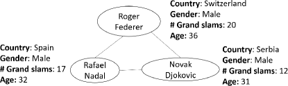
(a) Query

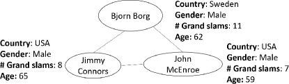
(b) Potential match

Figure 1. Two subgraphs from the Wikipedia knowledge graph. For simplicity, we drop the directionality and model them as an undirected graph.

One of the most common queries in these frameworks is to find similar embeddings of a query graph $q$ in a much larger target graph $G$. More formally, given a query graph $q$, a target graph $G$ and a similarity function $sim(q,g)$, the goal is to identify the top-$k$ most similar subgraphs $g\subseteq G$ to the query graph $q$. Traditional similarity functions consider two graphs as similar if they are structurally similar and they contain similar nodes(NEMA, ; NESS, ; ged_similarity1, ; node_embedding_similarity, ). Two nodes are said to be similar if they are represented by similar feature vectors; the most common form being just a node label. Despite significant advancements in the field of graph querying(deltacon, ; NEMA, ; ged_similarity1, ), this commonly adopted definition of similarity is oblivious to the presence of relationships in the graphs. In this work, we bring the power of relationships to graph querying.

To give an example of a relationship, consider the entity tuples $\langle$Rafael Nadal, Roger Federer$\rangle$ and $\langle$John McEnroe, Bjorn Borg$\rangle$ from the Wikipedia knowledge graph. Although the entities in these two tuples are different, both tuples encode a similar relationship; they represent players who played during the same era and won multiple grand slam tournaments between them. Annotating knowledge graphs with relationship information in the form of edge labels has been shown to expose a higher level of semantics than simple entity-to-entity matching(exemplar2, ; acl, ).

Fig. 1a presents a query subgraph from Wikipedia knowledge graph containing well-known tennis players of the current era. Wikipedia further characterizes each node with a bunch of summary features as shown in the figure. Now, consider the task of identifying a subgraph from Wikipedia similar to the query in Fig. 1a. Consider Fig. 1b, which depicts another group of well-known tennis players: Bjorn Borg, Jimmy Connors and John McEnroe. Would a tennis fan consider these two groups to be similar? There is a strong possibility that she would since both the groups respectively represent players who played during the same era and won multiple grand slam tournaments among them.

Let $g_{1}$ and $g_{2}$ be two graphs. Most of the existing techniques (NEMA, ; ctree, ; ged_similarity1, ; ged_similarity2, ; node_embedding_similarity, ) rely on mapping each node in $g_{1}$ to some node in $g_{2}$, and the cumulative similarity of the mapped node pairs dictate the overall similarity score between $g_{1}$ and $g_{2}$. When such a strategy is applied to the above two subgraphs (Fig. 1a and 1b), none of the possible node mappings would return a high score since their feature vectors are not similar. For example, Federer is not similar to any of the nodes in Fig. 1b, since he is from a different generation as indicated by his “Age”, and belongs to a different country. The “Gender” and “# Grand slams” will fetch some similarity, however, that may not be enough to offset the dissimilarity in the other two features. More fundamentally, although a graph contains a group/collection of nodes, existing techniques treat each node as an independent entity while comparing two graphs. Consequently, group-level relationships, that can be identified only by analyzing the group-level interactions between node feature vectors, are not reflected in the similarity score. For example, the relationship that each group contains players from roughly the same generation, as hinted by the “Age” feature, cannot be inferred through node similarity alone, where nodes are treated independently. This observation forms the core motivation behind our work to move beyond node similarity, and match subgraphs based on the relationships encoded through non-trivial interactions between node features.

Several important questions arise at this juncture. What is the precise definition of a relationship? How do we quantify the strength of a relationship? Are all relationships equally important? In this paper, we answer these questions. In sum, we make the following key contributions:

• We propose a novel graph querying paradigm, RAQ (Relationship-Aware Graph Querying), that incorporates the notion of relationship in its similarity function (Sec. 3). The proposed formulation automatically mines the relationships manifested in the query graph and ranks their importance based on their statistical significance (Sec. 4).

• We design the RAQ search algorithm, which employs beam stack search on an R-tree to identify good candidates. These candidates are further refined through neighborhood signatures constructed using random walks with restarts to prune the search space and compute the optimal answer set. (Sec. 5).

• Empirical evaluation (Sec. 6) on real datasets establishes three key properties. (1) RAQ produces results that are useful. This is validated by two user surveys. (2) RAQ complements existing graph similarity metrics by finding results that traditional techniques are unable to find. (3) RAQ is up to $5$ times faster than baseline strategies and scales to million-sized networks.

The code is available at: https://github.com/idea-iitd/RAQ.

2. Related Work

Research work done in both exact and approximate (sub-)graph querying have employed a plethora of similarity functions. The most prominent of them being graph edit distance (GED) (ged_similarity1, ; ged_similarity2, ), maximum and minimum common subgraph (mcg_similarity1, ; mcg_similarity2, ), edge misses (tale, ), structural similarity (best_effort, ; saga, ; isorank, ; NESS, ; NEMA, ; deltacon, ), node-label mismatches (saga, ; isorank, ), and statistical significance of node-label distributions (graphquerying_chi, ). However, all these methods operate oblivious to the presence of relationships in the query graph.

Query-by-example Paradigm: The need to query based on relationships is touched upon by the recent line of work on Query-by-example(exemplar, ; exemplar1, ; exemplar2, ; exemplar3, ). All these techniques take an edge or a set of edges as input, and this input is treated as an example of what the user wants to find. Each exemplar edge connects two entities of the knowledge graph and the edge label denotes the relationship between these entities. Typical relationships in a knowledge graph are “friendOf”, “locatedIn” etc. Given the exemplar edges, the common goal in this line of work is to identify subgraphs from the target graph that are connected by the same edge labels as expressed in the exemplars. Our work is motivated by the same line of thought and revamps this paradigm through the following innovations.

1. Mining relationships: While (exemplar, ; exemplar1, ; exemplar2, ; exemplar3, ) assume that relationships are explicitly provided in the form of edge labels, we mine these relationships from feature-value interactions observed between a pair of nodes. Thus, RAQ is not constrained by the explicit availability of edge relationships. This results in a more powerful model since it is hard to capture all possible relationships through a small set of edge labels. Furthermore, unlike existing query-by-example techniques, RAQ is not limited to edge-labeled (relationship-annotated) graphs alone, and exposes a more generic framework capable of operating on graphs with both node and edge labels.

2. Multiple relationships: Existing techniques assume each edge to be associated with only one relationship. In our formulation, each edge encodes $d$ relationships corresponding to each of the $d$ features characterizing a node.

3. Relationship importance: All relationships in the exemplar edges are assumed to be of equal importance. In the proposed paradigm, we analyze all of the identified relationships and quantify their importance through statistical significance. As we will see later in Sec. 6.3, users find this weighting relevant.

4. Relationship similarity: Existing query-by-example techniques are incapable of computing similarity between relationships. This is a natural consequence of the fact that relationships are reduced to categorical edge labels. Thus, relationships between two pairs of nodes are either considered identical or different. In contrast, RAQ is not limited to a binary matching. For example, the relationship with respect to “# Grand slams” between Federer and Nadal is similar to that between Bjorg and McEnroe, but not identical.

Overall, the proposed paradigm is more generic, and therefore more challenging to solve algorithmically.

3. Problem Formulation

The input to our problem is a target graph, a query graph, and the value $k$ corresponding to the top-$k$ matches that need to be identified.

Definition 1 (Target Graph).

The target graph $G=(V,E,\mathbb{F})$ contains a node set $V$, an edge set $E$, and a set of $d$-dimensional feature vectors $\mathbb{F}$, where each feature vector $f(v)=[f_{1}(v),\ldots,f_{d}(v)]$ characterizes a node $v\in V$. Optionally, each edge may also be annotated with an edge label.

Without loss of generality, we assume that for each feature value $f_{i}(v)$, $0\leq f_{i}(v)\leq 1$. A query graph $q=(V_{q},$ $E_{q}$, $\mathbb{F}_{q})$ follows the same notational structure as the target graph. Both the target graph and the query graph can be either directed or undirected. Our goal is to identify isomorphic embeddings of the query graph within the target graph, such that they encode relationships similar to that manifested in the query. Graph $g_{1}=(V_{1},$ $E_{1},$ $\mathbb{F}_{1})$ is isomorphic to $g_{2}=(V_{2},E_{2},\mathbb{F}_{2})$ if there exists a bijection $\phi$ such that for every vertex $v\in V_{1},\;\phi(v)\in V_{2}$ and for every edge $e=(u,v)\in E_{1},\phi(e)=(\phi(u),\phi(v))\in E_{2}$ and the labels of $e$ and $\phi(e)$ are the same. Among all isomorphic embeddings of the query graph $q$ in the target graph $G$, we want to select the $k$ embeddings that possess the highest relationship-aware similarity (RAS) to $q$ (defined formally in Def. 3).

Problem 1 (Top-$k$ Relationship-aware Querying).

Given a query graph $q$, a target graph $G$, and a positive integer $k$, identify the graphs $\mathbb{A}=\{g_{1},\cdots,g_{k}\}$, such that (1) $\forall g_{i}\in\mathbb{A},g_{i}$ is a subgraph of $G$, (2) $\forall g_{i}\in\mathbb{A},g_{i}$ is isomorphic to $q$, and (3) $\nexists g^{\prime}\subseteq G$ such that $RAS(g^{\prime},q)>RAS(g_{i},q)$ for some $g_{i}\in\mathbb{A}$.

The main task is to design the relationship-aware similarity function $RAS(g,q)$ for any two isomorphic graphs $g$ and $q$.

4. Relationship-aware Similarity

We first define what a relationship is. Intuitively, each feature represents the characteristics of a node and the relationship between two nodes is inferred by studying the interplay between their feature values. For example, considering Djokovic and Nadal, both entities are of the same gender, similar age, have won a large number of grand slam tournaments, but are citizens of different countries. Interactions between each corresponding feature of the connected nodes generate a relationship, and hence, a $d$-dimensional feature vector would produce $d$ relationships per edge. We capture these relationships in the form of a relationship vector $s(e)$ corresponding to each edge $e=(u,v)$.

Definition 2 (Relationship Vector).

The relationship vector, $s(e)$, of an edge $e=(u,v)$ captures the features that are preserved in the relationship between $u$ and $v$. Formally, $s(e)=[s(f_{1},e),\ldots,s(f_{d},e)]$ where

$$s(f_{i},e) =\begin{cases}\Gamma(f_{i}(u),f_{i}(v)),\quad\text{if}\quad f_{i}\text{ is real valued}\\ 1,\quad\text{if}\quad f_{i}\text{ is categorical and }f_{i}(u)=f_{i}(v)\\ 0,\quad\text{if}\quad f_{i}\text{ is categorical and }f_{i}(u)\neq f_{i}(v)\end{cases}$$

(1) $$\text{where }\Gamma(x,y) =\begin{cases}1,\quad\text{if }x=y=0\\ \min\{x,y\}/\max\{x,y\},\quad\text{otherwise }\end{cases}$$

Example 1.

The relationship vector $s(e)$ for the edge $e$ connecting Nadal and Djokovic in Fig. 1a is $[0,1,0.71,0.97]$. The second dimension is $1$ since it is a categorical feature and both are males. The third dimension is non-categorical and thus, the similarity between them is $\frac{12}{17}$. Similarly, the relationship vector of the edge between Connors and McEnroe in Fig. 1b is $[1,1,0.88,0.91]$.

From its definition, each dimension in the relationship vector takes a value in the range $[0,1]$. A value close to $1$ indicates that both endpoints of the edge share similar values. Two edges $e$ and $e^{\prime}$ are considered similar if they encode similar relationships. Thus, to quantify their similarity, we compute the similarity between their relationship vectors:

(2) $$eSim(e,e^{\prime}) =\sum_{i=1}^{d}w(i)\cdot\Gamma\left(s(f_{i},e),s(f_{i},e^{\prime})\right)$$

$eSim(e,e^{\prime})$ is a weighted min-max similarity between the two relationship vectors. The weight $w(i)$ of the $i^{\text{th}}$ relationship (feature) represents its relative importance with respect to the other relationships, and the function $\Gamma\left(s(f_{i},e),s(f_{i},e^{\prime})\right)$ operates as defined in Eq. 1. We add the constraint that $\sum_{i=1}^{d}w_{i}=1$.

Example 2.

Assume that each relationship is of equal importance and, therefore, $\forall i$, $w_{i}=\frac{1}{d}$. The similarity between the edges Nadal-Djokovic and Connors-McEnroe is, thus, $0.25\times 0+0.25\times 1+0.25\times\frac{0.71}{0.88}+0.25\times\frac{0.91}{0.97}=0.68$.

Given two isomorphic subgraphs $q$ and $g$, and an isomorphic mapping $\phi$ from the edges in $q$ to the edges in $g$, the relationship-aware similarity (RAS) with respect to the mapping $\phi$ is the similarity between the mapped edges from $q$ to $g$:

(3) $$RAS_{\phi}(q,g)=\sum_{\forall e_{q}=(u_{q},v_{q})\in E_{q}}eSim\left(e_{q},\phi(e_{q})\right)$$

Definition 3 (Relationship-aware Similarity).

The
relationship-aware similarity (RAS) between $q$ and $g$ is the maximum RAS under all possible isomorphic mappings:

(4) $$RAS(q,g)=\max_{\phi}\left\{RAS_{\phi}(q,g)\right\}$$

Quantifying Relationship Importance: The obvious question now is how to infer the weights in $eSim(e,e^{\prime})$ (Eq 2). One option is to ask the user to provide the weights. However, such a strategy may not be practical. Specifically, each edge may encode a large number of relationships corresponding to features characterizing the participating nodes, and providing a weight with respect to each relationship is hard for general users. Also, providing a large number of input parameters is a cumbersome procedure. Hence, ideally, the weights should be automatically inferred.

The simplest approach is to assume that all relationships are of equal importance, i.e. $\forall i,w_{i}=\frac{1}{d}$. This assumption however, may be unrealistic. To elaborate, is the relationship that both Nadal and Djokovic are males as important as the relationship that both of them have won a large number of grand slam tournaments? Intuitively, such an assumption appears to be odd.

More importantly, should the importance be constant under all situations and should it ignore the feature values. For example, consider an edge between two tennis players who have won no grand slams. In such a case, both would have a similarity of $1$ in the “# Grand Slams” dimension. In that case, is the importance of grand slams the same between these two players as compared to Nadal and Djokovic? From a human psychological point of view, we value events that are rare. The relationship between Nadal and Djokovic stands out since they have won so many grand slams. We capture this intuition through statistical significance. Higher the statistical significance of a relationship, more is its weight.

4.1. Statistical Significance of Relationships

Statistical significance tests quantify whether an event occurred due to chance alone or is a result of some additional factor. Several statistical tests exist (stattests, ), such as the chi-square test(graphchi, ), p-value(graphsig, ; pgraphsig, ; graphsig_jcim, ), g-test(leap, ), Kruskal-Wallis test, Anderson-Darling test, Shapiro-Wilk test, etc., to quantify the statistical significance of an event. However, none of the techniques work directly on both categorical data (e.g., country) as well as continuous-valued data (e.g., age). Thus, we need to either map continuous data into a discrete space or convert discrete, categorical data into a continuous domain. Since converting categorical data such as gender and country into a continuous space is not feasible, we discretize continuous data into bins. We use the chi-squared statistic (chi_square, ) to measure statistical significance since it is known to produce robust results (graphchi, ; stringchi, ) and is efficient to compute.

Converting continuous data into discrete bins has been extensively studied (survey, ). While any discretization technique can be used, we use kernel-density estimation based method (binning, ) since it is unsupervised and non-parametric and, therefore, easy to apply on any continuous valued variable.

Let $x$ be some event in a random experiment and $S$ be the sample space. For all outcomes $y\in S$, let $O_{y}$ represent the number of times outcome $y$ has occurred. The chi-square statistic, $X^{2}$, measures the statistical significance of the event $x$ through the deviation of the observed frequency of all possible outcomes $O_{y}$ from their expected frequency $E_{y}$ given by the null model:

(5) $$X^{2}=\sum_{\forall y\in S}\frac{(O_{y}-E_{y})^{2}}{E_{y}}.$$

The higher the chi-square, the more statistically significant the observed event is.

In our problem, an event corresponds to a relationship. A relationship is manifested in the form of feature values assumed by the two endpoints of an edge. Thus, we should compute the observed frequency of a relationship and compare it to its expected frequency as per the chi-square protocol. Towards that end, each edge $e=(u,v)$ gives rise to a relationship tuple $\tau=(f_{i}(u),f_{i}(v))$ corresponding to feature $f_{i}$. Let $\mathcal{V}(f_{i})$ represent the set of unique tuples assumed by feature $f_{i}$ across all edges in a graph $g$. Then, the observed frequency, $O_{\tau}$, for any relationship tuple $\tau\in\mathcal{V}(f_{i})$ is simply the number of times $\tau$ is encountered in $g$.

Example 3.

Let us revisit Fig. 1a. As a pre-processing step, we would first discretize “# Grand slams” and “Age” into discrete categories. Let us assume that grand slam wins are bucketed into the following bins – Poor: 0, Good: 1-5, Very Good: 6-10, Great: 11-15, All time great (ATG):$>15$. Therefore, $\mathcal{V}$( “# Grand slam”) contains the tuples (ATG,ATG) and (ATG,Great) with observed frequencies 1 and 2 respectively. Similarly, $\mathcal{V}$(“Gender”) $=\{(Male,Male)\}$, where observed frequency $O_{(Male,Male)}=3$.

Null Model: We assume that relationship tuples in the query graph are drawn independently and randomly from the distribution of tuples in the target graph $G$. If the distribution of a relationship tuple in the query graph deviates significantly from the distribution in target graph, we call the corresponding relationship statistically significant.

Let $P(f_{i})=\{p_{1},\ldots,$ $p_{|\mathcal{V}(f_{i})|}\}$ denote the probability distribution of relationship tuples for feature $f_{i}$ in the target graph $G=(V,E,\mathbb{F})$. Here, $p_{j}\in P(f_{i})$ represents the probability of finding tuple $\tau_{j}\in\mathcal{V}(f_{i})$ in the target graph and is equal to the ratio $\frac{freq(\tau_{j})}{|E|}$, where $freq(\tau_{j})$ denotes the frequency of tuple $\tau_{j}$ in the target graph. Since each relationship tuple of feature $f_{i}$ in the query graph is drawn randomly and independently from $P(f_{i})$, the expected frequency $E_{\tau}$ of any tuple $\tau$ in the query graph $q=(V_{q},E_{q},\mathbb{F}_{q})$ is

(6) $$E_{\tau}=|E_{q}|.p_{\tau}$$

The chi-square value of $f_{i}$ with observed frequency $O_{\tau}$ is, therefore,

(7) $$X^{2}_{f_{i}}=\sum_{\forall\tau\in\mathcal{V}(f_{i})}\frac{(O_{\tau}-E_{\tau})^{2}}{E_{\tau}}$$

Example 4.

Let us compute the significance of the grand slam and gender relationships in Fig. 1a. Since very few of the tennis players have won a grand slam tournament, we assume that in the target graph, $5\%$ of the edges have the relationship tuple (ATG, Great) and $1\%$ have the tuple (ATG, ATG). Therefore, the expected frequency of (ATG, Great), (ATG, ATG) and all other tuples in Fig. 1a is $0.05\times 3=0.15$, $0.01\times 3=0.03$ and $0.94\times 3=2.82$ respectively. Consequently,

$$X^{2}_{\#Grandslam}=\frac{(2-0.15)^{2}}{0.15}+\frac{(1-0.03)^{2}}{0.03}+\frac{(0-2.82)^{2}}{2.82}=57$$

In the gender relationship, let us assume that in the target graph $50\%$ of the edges contain the tuple (Male, Male), $40\%$ contain (Female, Female) and $10\%$ contain (Female, Male). Therefore, the expected frequency of (Male, Male), (Female, Female) and (Female, Male) in Fig. 1a are $1.5,1.2$ and $0.3$ respectively. Consequently, $X^{2}_{Gender}=3$. Therefore, we conclude that the grand slam relationship is much more significant than the relationship that all players are males.

Since the importance of each relationship is proportional to its statistical significance, the weight $w_{i}$ of the $i^{\text{th}}$ feature in Eq. (2) is

(8) $$w_{i}=\frac{X^{2}_{f_{i}}}{\sum_{j=1}^{d}X^{2}_{f_{j}}}$$

5. Relationship-Aware Querying (RAQ)

The naïve approach to solve a top-$k$ query is to first enumerate all possible subgraphs of the target graph, identify those that are isomorphic to the query, and then rank these isomorphic subgraphs based on their relationship-aware similarity. However, this approach is prohibitively expensive since the target graph contains exponential number of subgraphs. In fact, the problem is NP-complete since finding isomorphic embeddings of a query graph within the target graph reduces to subgraph isomorphism(ctree, ). We, therefore, need to design a more scalable searching algorithm.

5.1. Bottom-Up Exploration

We first analyze a bottom-up exploration strategy. First, we pick an arbitrary edge $e_{q}$ from the query graph $q$ and map it to an arbitrary edge $e$ of the target graph. We call $e_{q}$ the seed edge. This forms an $1$-edge common subgraph of $q$ and $G$. Next, we try to grow it into a $2$-edge subgraph by extending both $e_{q}$ and $e$ through one of their neighboring edges such that the two extended subgraphs are isomorphic and, therefore, a common subgraph of $q$ and $G$. This procedure of growing using a neighboring edge continues iteratively till either of the following two cases become true:

1. The subgraph cannot be grown any further such that it remains a subgraph of both $q$ and $G$. In this case, we fail to find an isomorphic embedding of $q$.

2. The subgraph becomes isomorphic to $q$. We compute its similarity to $q$ and store it as a candidate.

Once the growing procedure terminates, the search restarts by mapping the seed query edge to another edge of $G$.

Once all possible mappings of the seed edge are explored, we pick another query edge as the seed and repeat the procedure. Finally, the $k$ highest scoring isomorphic embeddings are returned.

The bottom-up exploration is brute-force in nature and explores all possible combinations. However, it offers some concrete directions to improve.

1. Seed selection: Can the seed edge be more strategically selected so that good candidates are found early?

2. Seed mapping: Can the seed edge be mapped to an edge $e$ in the target graph more intelligently so that with a high likelihood an isomorphic embedding is found around $e$, which is also highly similar to query graph $q$?

3. Pruning bad candidates: Can a candidate subgraph be pruned early by guaranteeing that it cannot be in the top-$k$?

5.2. Seed Selection and Mapping

Intuitively, we should explore the mapping that has the highest chance of growing into high-scoring isomorphic match to the query. An obvious approach is to compute edge similarity (Eq. 2) between all pairs of query edges and target graph edges, and choose the most similar pair. The computation cost for this is $O(|E_{q}|\cdot|E|)$. Since $|E|$ is a large number, we need a more efficient algorithm for this task. The similarity between two edges is essentially a weighted min-max similarity between two high-dimensional points, since each edge is represented by a $d$-dimensional relationship vector. Indexing high-dimensional points have been extensively studied (indexingbook, ), and we choose R-tree (rtree, ) for our framework. R-tree recursively partitions the entire dataset of relationship vectors into MBRs.

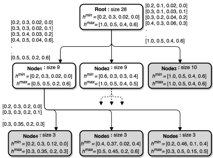
Figure 2. The structure of the R-tree. The leaf nodes are colored in grey. We do not explicitly show the relationship vectors in the leaf nodes due to space limitations.

Definition 4 (Minimum Bounding Rectangle, MBR).

Given a set of $d$-dimensional relationship vectors, $\mathbb{D}=\{s(e_{1}),\cdots,$ $s(e_{m})\}$, an MBR $\mathcal{H}$ on $\mathbb{D}$ is the smallest axis-parallel $d$-dimensional hyper-rectangle that encloses all vectors in $\mathbb{D}$.

An MBR $\mathcal{H}$ can be uniquely represented by the co-ordinates of its smallest and largest diagonal points $h^{min}$ and $h^{max}$ respectively. More specifically, $h^{min}=[h_{1}^{min},\ldots,h_{d}^{min}]$, where $h_{i}^{min}=\min_{\forall s(e)\in\mathbb{D}}\{s(f_{i},e)\}$, and $h^{max}$ is defined analogously. An example of an R-tree is shown in Fig. 2.

We use the notation $e\in\mathcal{H}$ to denote that the relationship vector $s(e)$ of $e$ is contained within MBR $\mathcal{H}$. Mathematically, this means $\forall i,\;h_{i}^{min}\leq s(f_{i},e)\leq h_{i}^{max}$. We define the similarity between a relationship vector $s(e_{q})$ of an edge $e_{q}$ and an MBR $\mathcal{H}$ as follows:

$$eSim(e_{q},\mathcal{H}) =\max_{\forall e\in\mathcal{H}}\{eSim(e_{q},e)\}$$

$$=\sum_{i=1}^{d}w(f_{i},e_{q})\cdot\max_{s(f_{i},e)\in[h_{i}^{min},h_{i}^{max}]}\left\{\Gamma(s(f_{i},e_{q}),s(f_{i},e))\right\}$$

Simply put, $eSim(e,\mathcal{H})$ provides the maximum similarity between $e$ and any possible edge contained within $\mathcal{H}$. This similarity value can be used to provide the following upper bound on $\mathbb{D}$.

Theorem 1.

If $\mathcal{H}$ is an MBR on a set of $d$-dimensional relationship vectors $\mathbb{D}$ and $e_{q}$ is a query edge then,

$$\max_{\forall s(e)\in\mathbb{D}}\{eSim(e_{q},e)\}\leq eSim(e_{q},\mathcal{H}).$$

We use Theorem 1 to search for the most similar edge to the query edge $e_{q}$ using the best-first search. Specifically, starting from the root node, we prioritize all child nodes based on the distance of their MBRs to the query edge. The best child node is then chosen to explore next and the process is recursively applied till we reach a leaf node (MBR without a child). Once a leaf node is reached, we compute the similarity to all nodes in this MBR and retain the highest scoring one. The best-first search procedure stops when all MBRs that remain to be explored have a maximum possible similarity smaller than the highest scoring target edge we have found till now. We discuss this more formally in Sec. 5.4.

5.3. Avoiding Local Maxima

While the above algorithm is efficient in locating a similar edge, it is prone to getting stuck in a local maxima. Specifically, searching for similar edges may lead us to a good match in a bad neighborhood (local maxima), and such leads should be avoided. A neighborhood is bad if one or both of the following are true:

1. The structure around the mapped edges is different.

2. The distributions of relationships around the mapped edges are different and, therefore, even if an isomorphic mapping is found, the similarity among the mapped edges (relationship vectors) is likely to be low.

Can we avoid dissimilar neighborhoods without explicitly performing isomorphism tests?

Neighborhood Signature: We answer the above question by mapping the neighborhood of an edge into a feature vector such that if two neighborhoods are similar, then their feature vectors are similar as well. This is achieved using Random Walks with Restarts (RWR). RWR starts from a source node and iteratively jumps from the current node to one of its neighbors with equal probability. To bound the walker within a $\delta$-hop neighborhood with a high likelihood, RWR employs a restart probability of $\alpha=\frac{1}{\delta}$. At any given state, with $\alpha$ probability, the walker returns to the source. Otherwise, the walker jumps to a neighbor.

Let $e$ be the edge whose neighborhood needs to be captured. We arbitrarily choose one of the endpoints of $e$ as the source node. RWR is initiated from it and for each edge $e^{\prime}$ that is traversed, a counter $c(e^{\prime})$ records the number of times $e^{\prime}$ have been traversed. The RWR is performed for a large number of iterations after which, we compute the neighborhood signature of edge $e$ as a $d$-dimensional feature vector $N(e)=[n_{1},\cdots,n_{d}]$, where

(9) $$n_{i}=\sum_{\forall e^{\prime}\in\mathbb{E}}\frac{c(e^{\prime})}{C}\times s(f_{i},e^{\prime})$$

where $\mathbb{E}$ is the set of all edges visited in the RWR and $s$ is as defined in Def. 2 and $C$ is the total number of iterations.

The signature captures the distribution of relationships around the source edge $e$. Edges that are closer to $e$ have a higher say. Consequently, the signature not only captures the relationship vectors in the neighborhood, but is also structure sensitive. While it is still possible for two dissimilar neighborhoods to have similar signatures, the chances that two dissimilar neighborhoods produce similar signatures across all $d$ dimensions is small.

We construct the neighborhood signature of all edges in the target graph as part of the index construction procedure. The signatures of the edges in the query graph are computed at query time. The neighborhood hop parameter $\delta$ is typically a small value since query graphs for knowledge discovery tasks are normally small(exemplar, ). In our empirical evaluation, we set $\delta$ to $3$.

5.4. RAQ Search Algorithm

Fig. 3 outlines the flowchart and Alg. 1 presents the pseudocode. There are three major phases: selecting the most promising query edge $e_{q}$ for exploration (seed selection phase), identifying the best matching target edges (seed mapping phase), and growing subgraphs from these initial seeds in bottom-up manner (growth phase).

Before we execute any of the phases, two operations are performed. First, we compute the neighborhood signatures of each edge in the query (line 1). Second, we use a priority queue called $Ans$, which stores the $k$ most similar subgraphs identified till now (line 2). Initially, $Ans$ is empty.

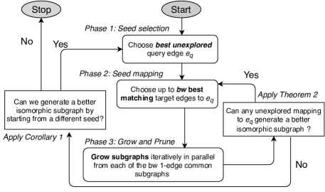
Figure 3. Flowchart of the searching algorithm in RAQ.

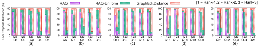
Figure 4. The distribution of the received user responses.

5.4.1. Phase 1: Seed Selection

We select the unexplored query edge $e_{q}\in E_{q}$ that has the highest similarity to the root node of R-tree (line 5). An edge is unexplored if it has not already been selected in this phase in some earlier iteration.

5.4.2. Phase 2: Seed Mapping

We use best-first search to find the leaf node in R-tree that has the highest similarity to $e_{q}$. In this leaf node, we perform a beam stack search(beamStackSearch, ) with beam width $bw$ (lines 13-20). Instead of mapping $e_{q}$ to the most similar target edge, beam stack search selects the $bw$ target edges that have the highest neighborhood similarity to $e_{q}$ and explores them further. The neighborhood similarity between two edges $e_{q}$ and $e$ is the weighted $L_{1}$ distance between their neighborhood signatures.

$$\text{Neighborhood\_Similarity}(e_{q},e)=\sum_{i}^{d}w_{i}\cdot\|N(i,e_{q})-N(i,e)\|$$

Recall that $w_{i}$ is the importance of the $i^{\text{th}}$ relation and more important relations have a higher say in defining the neighborhood similarity.

5.4.3. Phase 3: Grow and Prune

Each of the $bw$ edges selected in the previous phase generates a common 1-edge subgraph of the query and the target graph. We now grow them one edge at time to larger subgraphs (line 19). On any such subgraph $g=(V_{g},E_{g})$ we can apply the following bound.

Theorem 2.

The maximum similarity of any isomorphic match to query graph $q$ formed by growing $g$ further is $\widehat{RAQ}(q,$ $g)=RAQ(q,g)+|E_{q}|-|E_{g}|$.

Proof.

The maximum similarity between any two edges is $1$ (Eq. 2). Therefore, the maximum similarity contributed from the edges yet to be added is at most $|E_{q}|-|E_{g}|$. The theorem follows. ∎

Corollary 1.

Let $e_{q}$ be a query edge and $\mathcal{H}$ be an MBR in the R-tree. The maximum similarity of any isomorphic subgraph formed by mapping $e_{q}$ to any edge contained within $\mathcal{H}$ is $\widehat{RAQ}(e_{q},\mathcal{H})=eSim(e_{q},\mathcal{H})+|E_{q}|-1$.

Algorithm 1 RAQ Search Algorithm

0: $G=(V,E,\mathbb{F})$, $q(V_{q},E_{q},\mathbb{F}_{q}),\,k,RAQIndex$

0: Top-$k$ subgraphs of $G$ with highest relationship-aware similarity to $q$.

1: Compute neighborhood signature for each edge in $q$

2: $Ans\leftarrow\emptyset$ {Priority queue of maximum size $k$. Stores isomorphic matches in descending order of similarity.}

3: $Cands\leftarrow\emptyset$

4: while $\exists e\in E_{q},\;\widehat{RAQ}(e,rootNode.MBR)>Ans.leastValue()$ and $e$ has not been explored  do

5:    $e_{q}\leftarrow$ unexplored query edge with highest similarity to MBR in root node

6:    Initialize $Cands$ with the root node of R-tree

7:    while $Cands$ is not empty do

8:       $n\leftarrow Cands.poll()$

9:       $max\leftarrow\widehat{RAQ}(e_{q},n.MBR)$ .

10:       if $max\leq\allowbreak Ans.leastValue()$ then

11:          break

12:       if $n$ is a leaf node then

13:          while $\widehat{RAQ}(e_{q},n.MBR)>Ans.leastValue()$ and $n$ contains unexplored edges do

14:             $PQ\leftarrow$ Priority queue containing $bw$ unexplored edges with similar neighborhoods to $e_{q}$

15:             while $PQ$ is not empty do

16:                $g\leftarrow PQ.poll()$

17:                if $\widehat{RAQ}(g,q)\leq\allowbreak Ans.leastValue()$ then

18:                   break

19:                $\mathbb{G}\leftarrow$ Grow $g$ through all possible 1-edge extensions to form common subgraphs

20:                Add all isomorphic matches in $\mathbb{G}$ to $Ans$ and remaining subgraphs in $\mathbb{G}$ to $PQ$

21:       else

22:          Add all children of $n$ to $Cands$.

23: return  $Ans$

Equipped with the above upper bounds, we prioritize each of the initial 1-edge common subgraphs based on $\widehat{RAQ}(q,g)$ (Theorem 2). More specifically, we initialize another priority queue $PQ$ and insert all 1-edge subgraphs in $PQ$ (line 14). The subgraph $g$ with the highest upper bound is popped from $PQ$. We check if $\widehat{RAQ}(q,g)$ is larger than the $k^{\text{th}}$ highest similarity score in $Ans$ (line 17). If yes, we explore all possible single edge extensions of $g$ to create common subgraphs with one more edge (line 20). If $g$ becomes isomorphic to $q$ after extension, then we add it to $Ans$. Otherwise, we insert it back to $PQ$ (line 20). Otherwise, if the check (at line 17) fails, then we are guaranteed that none of the unexplored subgraphs in $PQ$ can lead to a better solution than what we already have and, hence, Phase 3 completes (lines 7-18).

5.5. Properties of RAQ Framework

Correctness Guarantee: The RAQ framework provides the optimal answer set. We do not prune off any possibility without applying Theorem 2 or Corollary 1. Consequently, we do not lose out on any candidate that can be in the top-$k$ answer set.

Index construction cost: The cost of constructing the R-tree is $O(d|E|\log(|E|))$. We also compute and store the neighborhood signature of each edge through random walk with restarts. This step can be performed in $O(|V|^{2})$ time for the entire graph(rwr, ; rwr1, ). Thus, the total computation cost is $O(|V|^{2}+d|E|\log(|E|))$.

Memory Footprint: R-tree consumes $O(d|E|)$ space since it stores $d$-dimensional relationship vectors of all edges. The neighborhood signatures are also $d$-dimensional feature vectors and hence the total cost is bounded by $O(d|E|)$.

Querying Time: As stated earlier, the problem is NP-complete. Hence, akin to most existing graph search algorithms(NEMA, ; exemplar, ; ctree, ), the worst case running time remains exponential. However, with the application of efficient heuristics and effective pruning bounds, we compute the top-$k$ answer set in milliseconds as elaborated next.

6. Experiments

Table 1. Summary of datasets used in our experiments.

Dataset	# Nodes	# Edges	Type	Mean Degree	# Features
IMDb	88K	781K	Undirected	17.59	7
DBLP	3.2M	6.8M	Directed	2.13	5
DBLP (co-author)	1.8M	7.4M	Undirected	8.44	5
Pokec	1.6M	30.6M	Directed	19.13	6

In this section, we evaluate the RAQ paradigm through user surveys, case studies, and scalability experiments.

6.1. Datasets

We consider a mix of various real (large) graphs (Table 1).

$\bullet$ The IMDb dataset (imdb, ) contains a collaboration network of movie artists, i.e., actors, directors, and producers. Each node is an artist featuring in a movie, and two artists are connected by an edge if they have featured together in at least one movie. Each node possesses $4$ features: (i) year of birth, (iii) the set of all the movies the artist has featured in, (iv) the most prevalent genre among his/her movies, and (v) the median rating of the movie set.

$\bullet$ The DBLP dataset (dblp, ) represents the citation network of research papers published in computer science. Each node is a paper and a directed edge from $u$ to $v$ denotes paper $u$ being cited by paper $v$. Each node possesses $5$ features: (i) publication venue, (ii) the set of authors, (iii) year of publication, (iv) the rank of the venue, and (v) the subject area of the venue. The publication year and venue rank are numerical features while the rest are categorical in nature. The first three features are obtained from the DBLP database while the last two are added from the CORE rankings portal (core_ranking, ).

$\bullet$ The DBLP (co-author) dataset (dblp, ) represents the co-authorship network of the research papers. Each node is an author of a paper and edges denote collaboration between two authors. Each node possesses $5$ features: (i) number of papers published by the author, (ii) the number of years for which the author has been active (calculated as the difference between the latest and the first paper), (iii) the set of venues in which the author has published, (iv) the set of subject area(s) of the venues in which the author has published, and (v) the median rank of the venue (computed as the median of the ranks of all the venues where the author has published). The number of papers published, number of years active, and the median rank are numerical features, while the rest are categorical.

$\bullet$ The Pokec dataset (snap, ) presents data collected from an on-line social network in Slovakia. Each node is a user of the social network and a directed edge $e=(u,v)$ denotes that $u$ has a friend $v$ (but not necessarily vice versa). Each node is characterized by six features: (i) gender, (ii) age, (iii) joining date, (iv) timestamp of last login (v) public: a boolean value indicating whether the friendship information of a user is public, and (vi) profile completion percentage. While public and gender are categorical features, the rest are numerical.

6.2. Experimental Setup

All experiments are performed using codes written in Java on an Intel(R) Xeon(R) E5-2609 8-core machine with 2.5 GHz CPU and 512 GB RAM running Linux Ubuntu 14.04.

Query graph: Query graphs are generated by selecting random subgraphs from the target graph. Following convention in graph querying (NEMA, ; exemplar, ), we considered queries with size up to $10$ edges. All reported results were averaged over $30$ random query graphs.

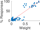
(a) Weight Correlation

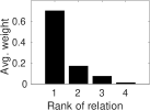
(b) Relation Weights

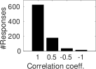
(c) Rank Correlation

Figure 5. (a) Correlation between weights and user-perceived relationship importance. Variation in (b) average weights from most to least important relationship, (c) Correlation across user responses.

Baselines: To measure the quality of graphs returned by RAQ, we compare its performance to three baselines:

$\bullet$ RAQ-uniform: To answer the question whether setting the weight of a relationship in proportion to its statistical significance helps, we implement RAQ-uniform as the setting where all relationships are considered equally important.

$\bullet$ Graph edit distance (GED): The edit distance between graphs $q$ and $g$ is the minimum cost of edits required to convert $q$ to $g$(ctree, ). An edit corresponds to deleting a node or an edge, adding a node or an edge, or substituting a node. Each edit has a cost. Deletions and additions of nodes or edges have a cost of $1$. The cost of substituting a node $u$ with $v$ is proportional to the distance between them. We use the min-max distance between the feature vectors of two nodes to compute the distance. The replacement cost $rep(u,v)$ is:

$$rep(u,v) =1-sim(u,v)$$

$$sim(u,v) =\frac{1}{d}\sum_{i=1}^{d}s_{i}(u,v)\qquad\text{where}$$

$$s_{i}(u,v) =\begin{cases}\frac{\min\{f_{i}(u),f_{i}(v)\}}{\max\{f_{i}(u),f_{i}(v)\}}\quad\text{if}\quad f_{i}\text{ is real valued}\\ 1\quad\text{if}\quad f_{i}\text{ is categorical and }f_{i}(u)=f_{i}(v)\\ 0\quad\text{if}\quad f_{i}\text{ is categorical and }f_{i}(u)\neq f_{i}(v)\end{cases}$$

$rep(u,v)$ is always within the range $[0,1]$.

$\bullet$ Query by example (QBE): We choose (exemplar1, ) to compare against the QBE paradigm (described in Sec. 2). To make it compatible to our framework, we model the node features as edge labels. Specifically, if $u$ and $v$ are connected in the original network, we introduce $d$ edges between them. The $i^{\text{th}}$ edge between $u$ and $v$ corresponds to the $i^{\text{th}}$ relationship (feature), and this relationship is captured in the form of edge label by concatenating the feature values $f_{i}(u)$ and $f_{i}(v)$. All numerical features are discretized into bins (binning, ) since otherwise, there would be infinitely many edge labels.

Parameters: The default value of $k$ in a top-$k$ query is set to $10$. The branching factor in R-tree is $b=4$.

6.3. User Survey: IMDb Dataset

To assess the relevance of the results retrieved using the proposed RAQ paradigm, we conducted two surveys spanning $170$ users each, using collaboration patterns (subgraph queries) from the IMDb dataset. The user-base was carefully chosen to ensure diversity in various aspects such as profession (engineers, researchers, homemakers, doctors, business executives etc.), educational background (from undergraduates to doctorates in science, engineering, medicine etc.), gender (approximately equal distribution between females and males), and age (from 20 to 70 years old). Each user was presented with $5$ queries randomly sampled from the master query pool, which led to a total of $850$ user-responses for each user survey. To enable the users in understanding the tasks better, they were briefed on the capabilities of the RAQ framework and the semantic interpretation of a graph.

Relationship Importance: The first user survey studies whether statistical significance is consistent with human intuition. For this, we constructed a query pool of $20$ edges (representing collaboration between two artists) along with their node features. For each query edge, we randomly choose two relationships (features), and the users were asked to identify the relatively more important relationship. A large number, $692/850$ ($81.4\%$), of the received user-responses considered the relationship with higher statistical significance to be more important. Considering the null hypothesis that either relationship is equally probable to be chosen as important, this observed outcome possesses a $p$-value of $1\mathrm{e}{-74}$ and is, therefore, highly statistically significant.

Moving ahead, we also analyze the correlation between the weight (normalized $X^{2}$ value) of a relationship and the proportion of times the feature is chosen as the preferred one in the survey. Fig. 5a shows that the higher the weight of a relationship, the more likely it is to be chosen as important in the user-responses. This is also indicated by their significantly high Pearson’s correlation coefficient (pearson, ) of $0.923$. Fig. 5b presents the average weight of the $k^{\text{th}}$ ranked feature, where $k$ is varied in the $x$-axis. We observe an exponential decay in weights, with the rank-$1$ relationship possessing a weight of $0.72$ on average. This result, in conjunction with Fig. 5a, shows that the highest ranked relationship has a much higher likelihood of being perceived as important in the user-responses. Overall, this survey provides substantive evidence to support the use of statistical significance in quantifying relationship importance.

Ranking Results based on Relevance: The second survey evaluates the relevance of the results retrieved by RAQ and the three baselines discussed above. For this task, we considered a query pool consisting of $25$ query subgraphs (representing group-level artist collaborations) possessing a judicious mix of node features (artist types, prominence, genres, etc.). For each query, the users were presented with top-$1$ results returned by the four algorithms being studied, and were asked to rank the results based on the user-perceived relevance to the query. To eliminate bias, the mapping of which result comes from which algorithm was masked from the user, and the order of the results presented were randomized. For ensuring simplicity and brevity, each query was annotated with the most important relationship, which was shown to correspond well with human perceived importance in the first survey.

Table 2. Comparing the quality of RAQ with the considered baselines using both user-level and query-level responses.

Retrieved	User-level Responses (%)				Query-level Responses (%)
Rank	RAQ	Uniform	GED		RAQ	Uniform	GED
1	86.0	10.6	3.4		100.0	0.0	0.0
2	10.0	75.4	14.6		0.0	92.0	8.0
3	4.0	14.0	82.0		0.0	8.0	92.0

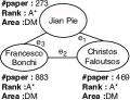
(a) Query 1

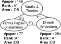
(b) Result 1

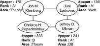
(c) Query 2

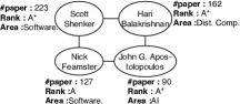
(d) Result 2

Figure 6. Matched subgraphs by RAQ.

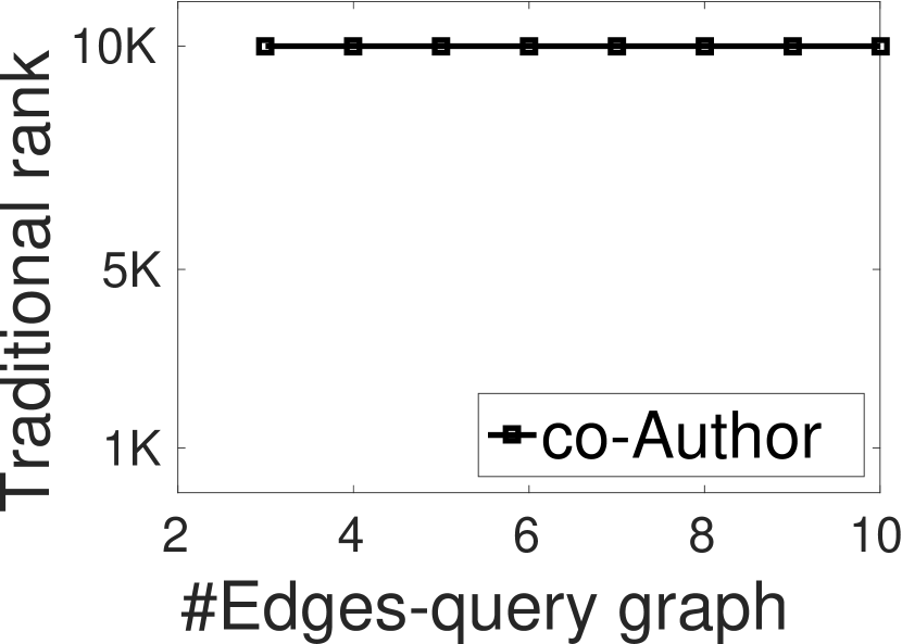
(a) RAQ vs GED

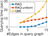
(b) IMDb

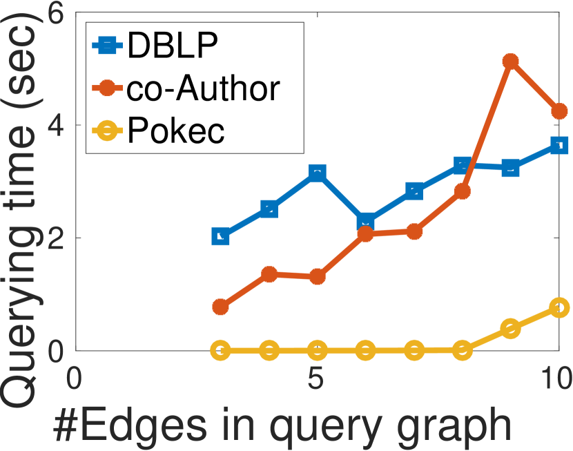
(c) Large datasets

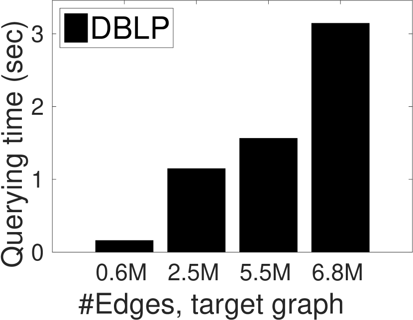
(d) DBLP

(e) Pokec

(f) DBLP

(g) Pokec

(h) Large datasets

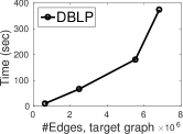
(i) DBLP

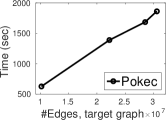
(j) Pokec

Figure 7. (a) Comparison of traditional graph search with the proposed relationship-aware similarity function. (b) Comparison of querying time between RAQ and the baseline technique. (c) Growth of querying time against query graph size and (d-e) target graph size. (f-g) Impact of target graph size on queries of various sizes. (h) Growth of querying time against $k$. (i-j) Growth of index construction time against network size.

Interestingly, across all $25$ queries, QBE returned an empty answer set since it did not find any subgraph from IMDb, other than the query itself, which had nodes connected by the same relationships as in the query. This result is not surprising. As we discussed in Sec. 2, QBE operates in a binary world where two relationships are either identical or different. This result indicates that while QBE is an intuitive and powerful framework for relationship-annotated knowledge graphs, it is not well-suited for graphs where the relationships are encoded through interactions between feature vectors characterizing each node. Owing to this result, the user survey reduced to a comparison among three techniques.

Table 2 summarizes the user responses and in Fig. 4, we plot the distribution of the received responses within each retrieved rank for each query. An overwhelming $731$ ($86\%$) of the $850$ received user responses deemed RAQ results to be the most relevant (rank-1 match) to the input query. Considering the null hypothesis where any one of the three results is equally likely to be chosen as the preferred one, this observed outcome is highly statistically significant ($p$-value of $2\mathrm{e}{-232}$). Moving beyond the analysis of rank-1 responses, we observe a high rank-correlation between the user-responses and the expected outcome, i.e., RAQ, RAQ-Uniform, and GED at ranks 1, 2, and 3 respectively, indicated by the average Spearman’s coefficient $\rho=0.803$(spearman, ). It is evident from Fig. 5c that $\approx 74\%$ of the user-responses perfectly match the expected output ranking with $\rho=1$.

In addition to analyzing the user-level responses, we performed a query-level analysis as well. Specifically, for each query-rank combination, we identified the algorithm preferred by the highest number of users. As is clear from Table 2, RAQ results were considered to be the most relevant (rank-1) for all $25$ ($100\%$) queries.

6.4. Case Study: DBLP Dataset

In this section, we showcase results from the DBLP co-author dataset and discuss how RAQ is able to identify relationship patterns that node-based distance measures like GED are unable to. Each node in this experiment is characterized by three features, number of papers published, median venue rank, and subject area. The subject area corresponds to the area of the venue where the author has published most of her works.

The query presented in Fig. 6a represents a collaboration pattern comprising prolific authors working in the field of data mining. Fig. 6b presents the matched subgraph by RAQ, which is a collaboration pattern among prolific authors working in the field of databases. As can be seen, all authors in Fig. 6b possess the median venue rank as “A*” and the subject area as “DB”. It is evident that RAQ captures the relationship that each group contains prolific authors from the same community. The result presented in Fig. 6b is not even within the top-10,000 matches produced by GED. This is natural since the two groups do not contain similar nodes.

Fig. 6c demonstrates RAQ’s ability to adapt with the query. More specifically, while the subject area was a preserved relationship in query 1, query 2 presents collaborations among authors with high paper counts, but from diverse backgrounds. The result, Fig 6d, is a collaboration pattern among authors from diverse backgrounds as well, but all prolific with a large number of papers.

Correspondence between RAQ and edit distance: In this section, we show that RAQ retrieves results that node-based techniques are unable to find. We perform a top-$5$ query on random query graphs with sizes varying from $3$ to $10$. For each of the top-$5$ RAQ results, we find its rank using GED. We plot the average rank in GED for each of the query graph sizes (Fig. 7a). Since it is hard to scale beyond top-10,000 in GED, if a RAQ result does not appear within top-10,000, we set its rank to 10,000. The GED rank of the top-5 RAQ matches is close to 10,000 on average. This behavior is not a coincidence. Node-based similarity functions match graphs by considering each node as an independent entity and remains blind to the patterns found when the nodes are considered as a group. Consequently, they miss out on similarities that RAQ is able to discover.

6.5. Efficiency and Scalability

We next compare the running time of RAQ with RAQ-uniform and QBE (exemplar1, ) (Fig. 7b). We omit GED since for query graphs sizes beyond 5 it is impractically slow. RAQ is up to 5 times faster than QBE which suffers due to replication of each edge $d$ times corresponding to $d$ relationships. RAQ is faster than RAQ-uniform, since in RAQ, the relationships weights are skewed. Hence, pruning strategies are more effective than RAQ-uniform, where all relationships are equally important.

Fig. 7c demonstrates the growth of querying time against query graph size. As expected, the growth of is exponential since the search space grows exponentially with query graph size. Nonetheless, RAQ limits the running time to a maximum of only 5 s.

Notice that RAQ is fastest in Pokec even though Pokec is the largest network containing more than $30$ million edges. The variance in feature values in Pokec is low. Consequently, the chance that a randomly picked subgraph is identical to the query is larger. Owing to this property, the search for the query graph converges quickly. Overall, these results establish that RAQ is a fast and practical search mechanism.

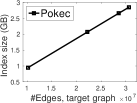
(a) Pokec

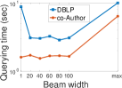
(b) Beam-width

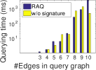
(c) RWR Signatures

Figure 8. (a) Growth of RAQ’s memory footprint against network size. Impact of (b) beam width and (c) neighborhood signatures on querying time.

Next, we study the impact of target graph size on the querying time. For this experiment, we extract four different subgraphs of the entire network covering $25\%$, $50\%$, $75\%$ and $100\%$ of the nodes (and all edges between them) of the entire network (Figs. 7d, 7e) In DBLP, the querying time increases with increase in target graph size. In Pokec, we do not observe a similar trend. Since we employ best-first search, the search procedure stops as soon as the upper bound of an unexplored candidate is smaller than the $k^{\text{th}}$ most similar subgraph we have already found. While an increase in target graph size increases the search space, it also enhances the chance of the $k^{\text{th}}$ subgraph being more similar and therefore an earlier termination of the best-first search. Due to this conflicting nature of our search operation, we do not see a consistent trend in the running time against the target graph size.

Figs. 7f and  7g study the impact of query graph size on the querying time. In general, we see any upward trend in the querying time as the size of the query graph increases.

Fig. 7h presents the variation of querying time across various values of $k$. We notice that the querying time flattens out very rapidly. This is due to the fact that the number of subgraphs explored till the answer set converges remains relatively same even for larger values of $k$.

Indexing Costs: Figs. 7i, 7j present the results of indexing costs on DBLP and Pokec. Even on Pokec, which contains more than $30$ million edges, RAQ completes index construction within $33$ minutes. RAQ index structures have a linear space complexity as reflected in Fig. 8a where we depict the memory footprint.

6.6. Optimization

The efficiency of the search algorithm RAQ is dependent on two major components: neighborhood signatures for identifying similar neighborhoods and beam-stack search to grow and prune initial candidates. In this section, we analyze their impact on RAQ.

Beam-width controls the number of simultaneous subgraphs we grow to form isomorphic matches to the query. We vary this parameter and plot the corresponding querying times in Fig. 8b. A beam width of $1$ reduces to depth-first search, where an initial bad choice needs to be explored till the end before moving to a different one. A larger beam width allows other promising candidates explored earlier. A very large value, however, keeps switching too often among the candidates. Overall, a beam width between $40$ and $60$ provides the highest speed-up.

We study the importance of neighborhood signatures. We compare the time taken for top-$k$ search using two techniques: RAQ with neighborhood prioritization through signatures and RAQ without neighborhood prioritization. Fig. 8c presents the results in the Pokec dataset. We observe that for smaller query graphs, RAQ without neighborhood optimization performs better. However, for larger query graphs neighborhood, typically, optimization helps. For smaller query graphs, the neighborhood of a query edge itself is very small and, thus, they lack much discriminative information. When the query size grows, the neighborhood of an edge is larger and the chances of getting stuck in a local maxima increases. Signatures allows us to escape these regions.

7. Conclusions

In this paper, we addressed the problem of graph querying under a novel Relationship-Aware Querying (RAQ) paradigm. RAQ captures the relationships present among nodes in the query graph and uses these relationships as an input to the similarity function. Majority of the existing techniques consider each node as an independent entity and, hence, remain blind to the patterns that exist among them when considered as a whole. RAQ not only mines these patterns in the form of relationships but also weighs their importance in proportion to their statistical significance. An overwhelming majority of $86\%$ of the users surveyed preferred RAQ over existing metrics. To address the computational challenges posed by graph querying, we designed a flexible searching algorithm, which performs beam-stack search on an R-tree to prune the search space. Empirical studies on real-world graph datasets established that RAQ is scalable and fast. Overall, RAQ opens a new door in the graph querying literature by surfacing useful results that would otherwise remain hidden.

References

- [1] Core rankings portal. http://portal.core.edu.au/conf-ranks/.
- [2] DBLP: Computer Science Bibliography. http://dblp.uni-trier.de/.
- [3] Facebook Graph Search. https://en.wikipedia.org/wiki/Facebook_Graph_Search.
- [4] Google Knowledge Graph. https://www.google.com/intl/es419/insidesearch/features/search/knowledge.html.
- [5] IMDB: The Internet Movie Data Base. https://www.imdb.com/interfaces/.
- [6] SNAP Datasets. https://snap.stanford.edu/data/.
- [7] A. Arora, M. Sachan, and A. Bhattacharya. Mining Statistically Significant Connected Subgraphs in Vertex Labeled Graphs. In SIGMOD, pages 1003–1014, 2014.
- [8] S. Auer, C. Bizer, G. Kobilarov, J. Lehmann, R. Cyganiak, and Z. Ives. Dbpedia: A nucleus for a web of open data. In ISWC, pages 722–735, 2007.
- [9] A. Bhattacharya. Fundamentals of Database Indexing and Searching. CRC Press, 2014.
- [10] M. Biba, F. Esposito, S. Ferilli, N. Di Mauro, and T. M. A. Basile. Unsupervised discretization using kernel density estimation. In IJCAI, pages 696–701, 2007.
- [11] K. Bollacker, C. Evans, P. Paritosh, T. Sturge, and J. Taylor. Freebase: A collaboratively created graph database for structuring human knowledge. In SIGMOD, pages 1247–1250, 2008.
- [12] H. Bunke and K. Shearer. A graph distance metric based on the maximal common subgraph. Pattern recognition letters, 19(3):255–259, 1998.
- [13] V. Chaoji, S. Ranu, R. Rastogi, and R. Bhatt. Recommendations to boost content spread in social networks. In WWW, pages 529–538, 2012.
- [14] S. Dutta, P. Nayek, and A. Bhattacharya. Neighbor-aware search for approximate labeled graph matching using the chi-square statistics. In WWW, pages 1281–1290, 2017.
- [15] C. Faloutsos, D. Koutra, and J. T. Vogelstein. DELTACON: A principled massive-graph similarity function. In SDM, pages 162–170, 2013.
- [16] M.-L. Fernández and G. Valiente. A graph distance metric combining maximum common subgraph and minimum common supergraph. Pattern Recognition Letters, 22(6):753–758, 2001.
- [17] A. Guttman. R-trees: A dynamic index structure for spatial searching. In SIGMOD, pages 47–57, 1984.
- [18] H. He and A. K. Singh. Closure-tree: An index structure for graph queries. In ICDE, 2006.
- [19] N. Jayaram, A. Khan, C. Li, X. Yan, and R. Elmasri. Querying knowledge graphs by example entity tuples. TKDE, 27(10):2797–2811, Oct 2015.
- [20] G. K. Kanji. 100 Statistical Tests. Sage, 2006.
- [21] A. Khan, N. Li, X. Yan, Z. Guan, S. Chakraborty, and S. Tao. Neighborhood based fast graph search in large networks. In SIGMOD, pages 901–912, 2011.
- [22] A. Khan, Y. Wu, C. C. Aggarwal, and X. Yan. Nema: Fast graph search with label similarity. PVLDB, 6(3):181–192, 2013.
- [23] S. Kotsiantis and D. Kanellopoulos. Discretization techniques: A recent survey.
- [24] M. Lissandrini, D. Mottin, T. Palpanas, and Y. Velegrakis. Multi-example search in rich information graphs. In ICDE, 2018.
- [25] D. Mottin, M. Lissandrini, Y. Velegrakis, and T. Palpanas. Exemplar queries: Give me an example of what you need. PVLDB, 7(5):365–376, 2014.
- [26] D. Mottin, M. Lissandrini, Y. Velegrakis, and T. Palpanas. Exemplar queries: a new way of searching. VLDBJ, 25(6):741–765, Dec 2016.
- [27] D. Natarajan and S. Ranu. A scalable and generic framework to mine top-k representative subgraph patterns. In 2016 IEEE 16th International Conference on Data Mining (ICDM), pages 370–379. IEEE, 2016.
- [28] D. Natarajan and S. Ranu. Resling: a scalable and generic framework to mine top-k representative subgraph patterns. Knowledge and Information Systems, 54(1):123–149, 2018.
- [29] G. Nikolentzos, P. Meladianos, and M. Vazirgiannis. Matching node embeddings for graph similarity. In AAAI, pages 2429–2435, 2017.
- [30] K. Pearson. Note on regression and inheritance in the case of two parents. Proceedings of the Royal Society of London, 58:240–242, 1895.
- [31] S. Ranu, B. T. Calhoun, A. K. Singh, and S. J. Swamidass. Probabilistic substructure mining from small-molecule screens. Molecular Informatics, 30(9):809–815, 2011.
- [32] S. Ranu, M. Hoang, and A. Singh. Answering top-k representative queries on graph databases. In Proceedings of the 2014 ACM SIGMOD international conference on Management of data, pages 1163–1174. ACM, 2014.
- [33] S. Ranu and A. K. Singh. Graphsig: A scalable approach to mining significant subgraphs in large graph databases. In 2009 IEEE 25th International Conference on Data Engineering, pages 844–855. IEEE, 2009.
- [34] S. Ranu and A. K. Singh. Mining statistically significant molecular substructures for efficient molecular classification. Journal of chemical information and modeling, 49(11):2537–2550, 2009.
- [35] S. Ranu and A. K. Singh. Indexing and mining topological patterns for drug discovery. In Proceedings of the 15th International Conference on Extending Database Technology, pages 562–565. ACM, 2012.
- [36] T. R. C. Read and N. A. C. Cressie. Goodness-of-fit Statistics for Discrete Multivariate Data. Springer, 1988.
- [37] M. Sachan and A. Bhattacharya. Mining statistically significant substrings using the chi-square statistic. In PVLDB, pages 1052–1063, 2012.
- [38] R. Singh, J. Xu, and B. Berger. Global alignment of multiple protein interaction networks with application to functional orthology detection. In PNAS, pages 12763–12768, 2008.
- [39] C. Spearman. The proof and measurement of association between two things. The American journal of psychology, 15(1):72–101, 1904.
- [40] Y. Tian, R. C. Mceachin, C. Santos, D. J. States, and J. M. Patel. Saga: A subgraph matching tool for biological graphs. Bioinf., 23(2):232–239, 2007.
- [41] Y. Tian and J. M. Patel. Tale: A tool for approximate large graph matching. In ICDE, pages 963–972, 2008.
- [42] H. Tong, C. Faloutsos, B. Gallagher, and T. Eliassi-Rad. Fast best-effort pattern matching in large attributed graphs. In KDD, pages 737–746, 2007.
- [43] H. Tong, C. Faloutsos, and J.-Y. Pan. Fast random walk with restart and its applications. In ICDM, pages 613–622, 2006.
- [44] N. Voskarides, E. Meij, M. Tsagkias, M. de Rijke, and W. Weerkamp. Learning to explain entity relationships in knowledge graphs. In ACL, 2015.
- [45] X. Yan, H. Cheng, J. Han, and P. S. Yu. Mining significant graph patterns by leap search. In Proceedings of the 2008 ACM SIGMOD International Conference on Management of Data, pages 433–444, 2008.
- [46] W. Yu and X. Lin. Irwr: incremental random walk with restart. In SIGIR, pages 1017–1020, 2013.
- [47] Z. Zeng, A. K. H. Tung, J. Wang, J. Feng, and L. Zhou. Comparing stars: On approximating graph edit distance. In PVLDB, pages 25–36, 2009.
- [48] W. Zheng, L. Zou, X. Lian, D. Wang, and D. Zhao. Graph similarity search with edit distance constraint in large graph databases. In CIKM, pages 1595–1600, 2013.
- [49] R. Zhou and E. A. Hansen. Beam-stack search: Integrating backtracking with beam search. In ICAPS, pages 90–98, 2005.