Many-body spectral functions from steady state density functional theory

Abstract

We propose a scheme to extract the many-body spectral function of an interacting many-electron system from an equilibrium density functional theory (DFT) calculation. To this end we devise an ideal scanning tunneling microscope (STM) setup and employ the recently proposed steady-state DFT formalism (i-DFT) which allows to calculate the steady current through a nanoscopic region coupled to two biased electrodes. In our setup one of the electrodes serves as a probe (’STM tip’), which is weakly coupled to the system we want to measure. In the ideal STM limit of vanishing coupling to the tip, the system is restored to quasi-equilibrium and the normalized differential conductance yields the exact equilibrium many-body spectral function. Calculating this quantity from i-DFT, we derive an exact relation expressing the interacting spectral function in terms of the Kohn-Sham one. As illustrative examples we apply our scheme to calculate the spectral functions of two non-trivial model systems, namely the single Anderson impurity model and the Constant Interaction Model.

Density functional theory (DFT)Hohenberg and Kohn (1964); Kohn and Sham (1965); Dreizler and Gross (1990) is without doubt one of the most popular and succesful approches for the description of matter, with important applications in condensed matter physics, material science and computational chemistry. DFT owes its success to its relative simplicity and low computational cost as compared to other approaches for solving the quantum many-body problem. Despite its simplicity, DFT is in principle exact, i.e., it can provide the exact ground state energy and density of many-electron systems. In practice, of course, an approximation for the exchange correlation (xc) energy functional is needed and a plethora of such approximations have been suggested Kohn and Sham (1965); J.P. Perdew and Wang (1986); A.D. Becke (1988); Lee et al. (1988); A.D. Becke (1993); J.P. Perdew et al. (1996, 1999); Tao et al. (2003); Kümmel and Kronik (2008).

Via the Hohenberg-Kohn theorem Hohenberg and Kohn (1964) the ground state density uniquely determines the external potential (up to a constant). Therefore the many-electron Hamiltonian and thus all physical properties of the interacting system (including, e.g., excitation energies or spectral functions) are determined in principle uniquely by the ground state density. In practice, of course, this functional dependence is unknown and these quantities have to be extracted from some alternative theoretical framework. While optical excitations can successfully be computed within time-dependent DFT (TDDFT) Runge and E.K.U. Gross (1984); Ullrich (2012); Maitra (2016), spectral functions which encode information about the (quasi-particle) excitations of the system (energies and lifetimes) have so far been out of reach for DFT and instead are typically calculated with a Green function framework Onida et al. (2002); Martin et al. (2016). Spectral functions to a large degree determine the transport properties of a many-electron system and can (approximately) be measured, e.g., with STM spectroscopy or angular resolved photoemisson spectroscopy (ARPES).

Despite the lack of a formal justification, the eigenvalues of the fictitious non-interacting Kohn-Sham (KS) system Kohn and Sham (1965) of DFT are often used as an approximation for the quasi-particle band structures of solids. This approach works reasonably well for weakly correlated systems, but fails for strongly correlated ones. An extreme case is the one of the Mott-Hubbard insulator for which the KS spectrum predicts a metallic ground state, even when using the exact xc functional Capelle and Campo Jr. (2013).

In the present work we describe a scheme to extract the interacting spectral function (and thus an excited state property) essentially from a ground state DFT calculation. In order to do so, we need to make use of a recently proposed DFT framework for non-equilibrium steady state transport, the so-called i-DFT approach Stefanucci and Kurth (2015); Kurth and Stefanucci (2017). Under certain, well-defined conditions (see below) the i-DFT self-consistent equations for density and current decouple. While the one for the density becomes equivalent to the usual ground-state DFT selfconsistency condition, the extra equation for the current can be used to extract the spectral function.

The basic idea is to ’measure’ the spectral function of a system by means of an STM like setup where a small portion of the system ($S$) is probed by an STM tip ($T$), as shown in the left panel of Fig. 1. The tip couples only very weakly to the sample $S$ and thus does not influence the system in an essential way. Hence the system $S$ to be probed is essentially in equilibrium with electrode $R$. In addition, we assume that the applied bias $V$ drops entirely at the STM tip. Then the Keldysh Green function (GF) Stefanucci and van Leeuwen (2013) of the sample region becomes independent of the bias. Thus the density matrix $\bm{\rho}$ of $S$, and correspondingly the particle density $n(\bm{r})=\sum_{m,m^{\prime}}\phi^{\ast}_{m}(\bm{r})\rho_{mm^{\prime}}\phi_{m^{\prime}}(\bm{r})$ (where the $\phi_{m}(\bm{r})$ form a single-electron basis spanning $S$) are also independent of $V$, $\partial{\bm{\rho}}/\partial{V}=0$, and can be calculated from the equilibrium expression,

$$\bm{\rho}=-2i\,\int\frac{d\omega}{2\pi}\bm{G}^{<}(\omega)\xrightarrow[{\bm{\Gamma}}_{\rm T}\to 0]{}2\,\int\frac{d\omega}{2\pi}\,f(\omega)\,\bm{A}(\omega)$$ (1)

where $\bm{G}^{<}$ is the lesser GF matrix, $\bm{A}\equiv{i(\bm{G}^{a}-\bm{G}^{r})}$ the spectral function, $\bm{G}^{a}$ and $\bm{G}^{r}$ the retarded and advanced GF matrices, respectively, and $f(\omega)$ the Fermi function of $S$+$R$ with chemical potential $\mu\equiv 0$.

The current from the tip to the sample is given by the Meir-Wingreen expression Meir and Wingreen (1992):

$$I(V)=2\,\int\frac{d\omega}{2\pi}\,{\rm Tr}\left\{f_{\rm T}(\omega)\,{\bm{\Gamma}}_{\rm T}\,\bm{A}(\omega)+i{\bm{\Gamma}}_{\rm T}\,\bm{G}^{<}(\omega)\right\}$$ (2)

where $f_{\rm T}(\omega)=f(\omega-V)$ and we have defined the coupling matrix $\bm{\Gamma}_{\alpha}=i(\bm{\Sigma}_{\alpha}^{\dagger}-\bm{\Sigma}_{\alpha})$ of lead $\alpha$ ($\alpha={\rm T,R}$ for tip and rest, respectively) expressed in terms of the corresponding embedding self energy $\bm{\Sigma}_{\alpha}$.

By taking the derivative of Eq. (2) w.r.t. $V$ in the ideal STM limit of vanishing coupling to the tip, ${\bm{\Gamma}}_{\rm T}\rightarrow 0$, and with $V$ dropping entirely at the tip, we find that the differential conductance can be expressed solely in terms of the equilibrium spectral function of the sample:

$$\frac{\partial{I}}{\partial{V}}\xrightarrow[{\bm{\Gamma}}_{\rm T}\to 0]{}\int\frac{d\omega}{\pi}\,\frac{\partial{f_{\rm T}}}{\partial{V}}\,{\rm Tr}\left[{\bm{\Gamma}}_{\rm T}\bm{A}(\omega)\right]\xrightarrow[T\to 0]{}\frac{{\rm Tr}\left[{\bm{\Gamma}}_{\rm T}\bm{A}(V)\right]}{\pi}$$ (3)

where in the last step we have used that in the zero-temperature limit $T\rightarrow 0$ the derivative of the Fermi function becomes a $\delta$-function, $\partial{f_{\rm T}}/\partial{V}=-f^{\prime}(\omega-V)\rightarrow\delta(\omega-V)$. Eq. (3) holds for arbitrary coupling ${\bm{\Gamma}}_{\rm T}$ to the tip. By choosing the coupling matrix such that only a single matrix element is nonvanishing, i.e., ${\bm{\Gamma}}_{\rm T}=\gamma^{{\rm T}}_{lm}\left|l\right\rangle\left\langle m\right|$, one can thus extract an arbitrary matrix element of the (many-body) spectral function matrix as

$$A_{ml}(\omega)=\lim_{\gamma^{{\rm T}}_{lm}\to 0}\frac{\pi}{\gamma^{{\rm T}}_{lm}}\left.\frac{\partial{I}}{\partial{V}}\right|_{V=\omega}$$ (4)

provided that the $I-V$ characteristic of the interacting system is known.

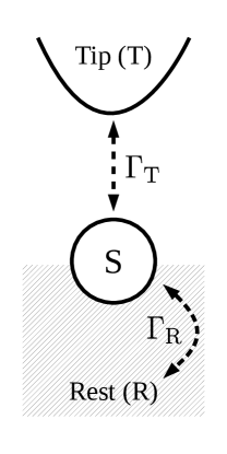
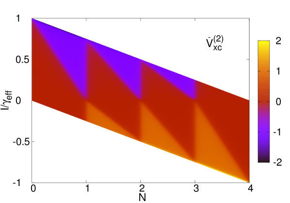
Figure 1: Left: STM like theoretical setup for measuring the true many-body spectral function of a system in a density functional theory framework. The tip (T), couples very weakly to the sample (S), which in turn is strongly coupled to the rest of the system (R). Right: xc bias $\bar{V}_{\rm xc}^{(2)}$ of Eq. (13) for the CIM with $\mathcal{M}=2$ and $U/\gamma=5$.

Here we choose a recently proposed density functional theory for steady-state transport Stefanucci and Kurth (2015), named i-DFT, as the framework for calculating the steady current $I$ and then exploit Eq. (4) to extract the spectral function. The central idea of i-DFT is that the pair of “densities” $(n(\bm{r}),I)$ of the interacting system can in principle exactly be reproduced by an effective system of non-interacting electrons, the KS system. This KS system features both a local Hartree-exchange-correlation (Hxc) potential $v_{\rm Hxc}[n,I](\bm{r})$ in $S$ as well as a (spatially constant) exchange-correlation (xc) contribution $V_{\rm xc}[n,I]$ to the bias. Both these (H)xc potentials are functionals of the density $n(\bm{r})$ in $S$ and the steady current $I$.

Originally, the self-consistent KS equations of i-DFT for the steady state density and current were formulated for the situation of a bias applied symmetrically in both leads Stefanucci and Kurth (2015) but they are easily transformed to the situation where the applied bias $V$ drops entirely at the tip. For this asymmetrically applied bias and arbitrary couplings ${\bm{\Gamma}}_{\rm T}$ and ${\bm{\Gamma}}_{\rm R}$ to the electrodes, the self-consistent i-DFT KS equations read

$$n(\bm{r}) = 2\int\frac{d\omega}{2\pi}\left[f(\omega-V_{s})A_{{\rm T},s}\left(\bm{r};\omega\right)+f(\omega)A_{{\rm R},s}\left(\bm{r};\omega\right)\right]$$

$$I = 2\,\int\frac{d\omega}{2\pi}\,[f(\omega-V_{s})-f(\omega)]\,T_{s}\left(\omega\right)\hskip 4.30554pt$$ (5b)

where $\bm{A}_{\alpha,s}=\bm{G}_{s}\bm{\Gamma}_{\alpha}\bm{G}_{s}^{\dagger}$ is the non-equilibrium KS spectral function of $S$ associated with electron injection from electrode $\alpha$, $A_{\alpha,s}(\bm{r};\omega)=\left\langle\bm{r}\right|\bm{A}_{\alpha,s}(\omega)\left|\bm{r}\right\rangle$ its spatial representation. $T_{s}={\rm Tr}[{\bm{\Gamma}}_{\rm T}\bm{G}_{s}^{\dagger}{\bm{\Gamma}}_{\rm R}\bm{G}_{s}]$ is the KS transmission function and $\bm{G}_{s}=(\omega-\frac{V_{\rm xc}}{2}-\bm{h}_{s}-\bm{\Sigma}_{\rm T}-\bm{\Sigma}_{\rm R})^{-1}$ is the (retarded) non-equilibrium KS Green function of the sample region. Here $\bm{h}_{s}=\bm{t}+\bm{v}_{s}$ is the KS Hamiltonian in matrix notation with $\bm{t}$ the kinetic energy and $\bm{v}_{s}$ the KS “gate” potential which, in the position basis is given as usual by $v_{s}(\bm{r})=v(\bm{r})+v_{\rm Hxc}(\bm{r})$. $V_{s}=V+V_{\rm xc}$ is the effective KS bias containing both the externally applied bias $V$ and the xc bias $V_{\rm xc}$. Note that here the frequency dependence of the embedding self energies and the corresponding coupling matrices is given by $\bm{\Sigma}_{\rm T}=\bm{\Sigma}_{\rm T}(\omega-V_{s})$ for the tip and $\bm{\Sigma}_{\rm R}=\bm{\Sigma}_{\rm R}(\omega)$ for the rest where $\bm{\Sigma}_{\alpha}(\omega)$ is the embedding energy of lead $\alpha$ in equilibrium.

In the ideal STM limit, ${\bm{\Gamma}}_{\rm T}\rightarrow 0$, the i-DFT expression (5) for the density reduces to $n(\bm{r})=2\,\int\frac{d\omega}{2\pi}\,f(\omega)A_{{\rm R},s}(\bm{r};\omega)$. As we have seen in Eq. (1), in this limit the density matrix and thus the density take on their equilibrium values and become independent of the applied bias, $\partial{n}(\bm{r})/\partial{V}=0$. The equilibrium density can be expressed in terms of the equilibrium KS spectral function $A_{s}^{(0)}(\omega)$ as

$$n(\bm{r})=\int\frac{d\omega}{\pi}\,f(\omega)A_{s}^{(0)}(\bm{r};\omega)\;.$$ (6)

Since the equilibrium Hxc potential $v_{\rm Hxc}^{(0)}[n](\bm{r})$ which yields the exact equilibrium density is unique, we can thus deduce the following important relationship between the xc bias and Hxc gate:

$$\lim_{{\bm{\Gamma}}_{\rm T}\rightarrow 0}v_{\rm Hxc}[n,I](\bm{r})+\frac{1}{2}V_{\rm xc}[n,I]=v_{\rm Hxc}^{(0)}[n](\bm{r})\;.$$ (7)

As a consequence of the ideal STM limit, the i-DFT equation for the density is completely decoupled from the current and can be solved at equilibrium, i.e. within a normal ground state KS DFT calculation. Furthermore, for ${\bm{\Gamma}}_{\rm T}\rightarrow 0$ the transmission function reduces to an expression similar to Eq. (3), i.e., $T_{s}\rightarrow{\rm Tr}[{\bm{\Gamma}}_{\rm T}\bm{A}_{s}^{(0)}]$, where $\bm{A}_{s}^{(0)}(\omega)$ is the equilibrium KS spectral function. For the tip coupling matrix we again take ${\bm{\Gamma}}_{\rm T}=\gamma^{{\rm T}}_{lm}\left|l\right\rangle\left\langle m\right|$ and, using Eq. (7), obtain

$$\lim_{\gamma^{\rm T}_{lm}\to 0}\frac{I}{\gamma^{\rm T}_{lm}}=\int\frac{d\omega}{\pi}\,[f(\omega-V-V_{\rm xc})-f(\omega)]\,A_{ml,s}^{(0)}(\omega)\;.$$ (8)

Note that the dependence on the bias shows up explicitly in the Fermi function of the tip and implicitly in the xc bias $V_{\rm xc}$ which depends on the current. In other words, for a given external gate potential (and thus at fixed equilibrium density $n(\bm{r})$ and KS spectral function $\bm{A}_{s}^{(0)}(\omega)$), Eq. (8) becomes a self-consistency condition for the current. From Eq. (8) we can calculate the differential conductance and, via Eq. (4), determine the many-body spectral function in the limit of zero temperature. Taking the derivative of Eq. (8) w.r.t. $V$ in the zero temperature limit yields

$$A_{ml}(\omega)=\lim_{\gamma^{\rm T}_{lm}\to 0}\left(1+\frac{\gamma_{lm}^{\rm T}}{\pi}\frac{\partial{V_{\rm xc}}}{\partial{I}}A_{ml}(\omega)\right)A_{ml,s}^{(0)}(\omega+V_{\rm xc})\;.$$ (9)

where we have taken into account that $V_{\rm xc}$ depends on $I$. Solving for $A_{ml}(\omega)$ we arrive at the central result of our paper which relates the many-body spectral function to the equilibrium KS spectral function:

$$A_{ml}(\omega)=\lim_{\gamma^{\rm T}_{lm}\to 0}\frac{A_{ml,s}^{(0)}(\omega+V_{\rm xc})}{1-\frac{\gamma_{lm}^{\rm T}}{\pi}\frac{\partial{V_{\rm xc}}}{\partial{I}}A_{ml,s}^{(0)}(\omega+V_{\rm xc})}$$ (10)

The xc bias $V_{\rm xc}$ and its derivative $\partial{V_{\rm xc}}/\partial{I}$ are to be evaluated with the current $I$ obtained by solving Eq. (8) at bias $V=\omega$. The appearance of $\gamma^{\rm T}_{lm}$ as prefactor of the second term in the denominator of Eq. (10) does not imply that this term vanishes in the limit $\gamma^{\rm T}_{lm}\to 0$ since $\frac{\partial{V_{\rm xc}}}{\partial{I}}$ diverges as $1/\gamma^{\rm T}_{lm}$ (see example for $V_{\rm xc}$ below). We emphasize that Eq. (10) is an exact result provided that the exact functionals $v_{\rm Hxc}[n]$ and $V_{\rm xc}[n,I]$ are used. In practice, of course, these functionals are unknown and need to be approximated (see below). The proposed scheme to calculate the spectral function is computationally very efficient: it requires only the usual KS self-consistency for the density plus, for any frequency (bias), the solution of Eq. (8) for the current. Eq. (10) expresses the equilibrium spectral function as functional of the ground state density using concepts of i-DFT (the xc bias $V_{\rm xc}$). This is similar to TDDFT in the linear regime where the linear density response function is a functional of the ground state density expressed in terms of the (frequency-dependent) xc kernel, a pure TDDFT quantity.

In the following we apply our formalism to model systems $S$ to be probed by the STM setup. We model $S$ as a quantum dot described by the constant interaction model (CIM) for which the Hamiltonian is $\hat{H}^{\rm CIM}=\sum_{i\sigma}\varepsilon_{i}\hat{n}_{i\sigma}+U/2\sum_{i\sigma\neq j\sigma^{\prime}}\hat{n}_{i\sigma}\hat{n}_{j\sigma^{\prime}}$ where $\hat{n}_{i\sigma}$ is the electron occupation operator for level $i$ with spin $\sigma$. The system $S$ is connected to both a tip $T$ and a second lead $R$ via energy independent couplings $\Gamma_{\alpha}$, i.e., we are in the wide-band limit (WBL) for both leads. Note that for a single level this becomes the single-impurity Anderson model (SIAM) Anderson (1961). The CIM has been studied within the i-DFT framework both in the Coulomb blockade Stefanucci and Kurth (2015) as well as in the Kondo regime Kurth and Stefanucci (2016, 2017) and approximate i-DFT xc potentials have been suggested. For simplicity, we restrict ourselves to the CIM with an arbitrary number $\mathcal{M}$ of degenerate single-particle levels ($\varepsilon_{i}=\varepsilon$) which are all coupled in the same way to the lead $\alpha$ , i.e., the coupling matrices in the single-particle basis $\Gamma_{\alpha}=\gamma^{\alpha}{\mathbf{1}}$ are proportional to the unit matrix $\mathbf{1}$ (the constants $\gamma^{\rm T}$ and $\gamma^{\rm R}$ can differ). In this case the i-DFT xc potentials depend only on the total number $N=\sum_{i\sigma}n_{i\sigma}$ of electrons on the dot.

We need to solve the usual DFT self-consistency for the ground state density and, as usual, in order to do so we need an approximation for the Hxc potential $v^{(\mathcal{M})}_{\rm Hxc}[N]$ of the degenerate ${\mathcal{M}}$-level CIM. The general structure of this potential is clear: $v^{(\mathcal{M})}_{\rm Hxc}[N]$ will exhibit steps of height $U$ at integer $N$. In the language of DFT, the height $U$ of these steps can be identified with the famous derivative discontinuity of the xc energy functional Perdew et al. (1982). For the uncontacted CIM at zero temperature, the exact Hxc potential is discontinuous Stefanucci and Kurth (2013) but when the CIM is brought in contact with (wide band) leads, these discontinuities are smoothened, the smoothening governed by the parameter $\gamma=\gamma^{\rm R}$. In the present work we use for $v^{(\mathcal{M})}_{\rm Hxc}[N]$ the form suggested in Eqs. (143) and (144) of Ref. Kurth and Stefanucci (2017) which consists of a sum of accurately parametrized Hxc potentials for the SIAM Bergfield et al. (2012).

We still need an approximate functional for the xc bias $V^{(\mathcal{M})}_{\rm xc}[N,I]$ of the degenerate ${\mathcal{M}}$-level CIM in the limit $\gamma^{\rm T}\to 0$. Below we propose an approximation and discuss the various ideas entering in its construction. Our approximate functional reads

$$V^{(\mathcal{M})}_{\rm xc}[N,I]=(1-a[I])\bar{V}^{(\mathcal{M})}_{\rm xc}[N,I]\;.$$ (11)

where $a[I]$ is a purely current-dependent function for which we choose the form

$$a[I]=1-\frac{2}{\pi}\arctan\left[\lambda\left(\frac{I}{W\gamma_{\rm eff}}\right)^{2}\right]$$ (12)

with the parameters $\lambda=0.16$, $\gamma_{\rm eff}=\frac{4\gamma^{\rm T}\gamma^{\rm R}}{\gamma^{\rm T}+\gamma^{\rm R}}$ and $\bar{V}^{(\mathcal{M})}_{\rm xc}[N,I]$ given as

$$\bar{V}^{(\mathcal{M})}_{\rm xc}[N,I]=-\sum_{K=1}^{2\mathcal{M}-1}U\sum_{s=\pm}\frac{s}{\pi}\,{\rm atan}\left(\frac{\Delta_{K}^{(s)}(N,I)}{2W}\right)$$ (13)

with $W=0.16\gamma/U$. The $\Delta_{K}^{(s)}(N,I)$, $s=\pm$, are piecewise linear functions of $N$ and $I$. For $s=+$ they are independent of the current and read

$$\Delta_{K}^{(+)}(N,I)=N-K$$ (14)

while for $s=-$ the corresponding form is

$$\Delta_{K}^{(-)}(N,I)=\left\{\begin{array}[]{cl}N+\alpha_{K}^{(+)}\frac{I}{4\gamma^{\rm T}}-K&\mbox{for $I\geq 0$}\\ N+\alpha_{K}^{(-)}\frac{I}{4\gamma^{\rm T}}-K&\mbox{for $I<0$}\end{array}\right.$$ (15)

The constants $\alpha_{K}^{(s)}$, $s=\pm$, are given by

$$\alpha_{K}^{(+)}=\frac{4}{2\mathcal{M}-K+1}\hskip 4.30554pt\mbox{ and }\hskip 4.30554pt\alpha_{K}^{(-)}=\frac{4}{(K+1)}\;.$$ (16)

For completeness we note the convention used throughout that a positive current flows from the tip $T$ to the sample $S$.

Where do the different ingredients for the xc bias come from? In Ref. Stefanucci and Kurth (2015) we constructed xc functionals for the Coulomb blockade regime for a symmetrically coupled, degenerate $\mathcal{M}$-level CIM by numerical inversion of rate equations Beenakker (1991). The resulting xc potentials showed a complex pattern of smeared steps of height $U/2$ for the Hxc gate and height $U$ for the xc bias potential. The position of the steps is determined by piecewise linear functions connecting vertices in the $N-I$ plane where the vertices correspond to $(2\mathcal{M}+1)^{2}$ plateau values of density and current in a scan over gate and bias. Here we are interested in the situation of a CIM with completely asymmetric coupling $\gamma^{\rm T}\to 0$. By analyzing the rate equations in this case we found that (i) the codomain of the Hxc potentials becomes a parallelogram connecting the points $(N,I/\gamma_{\rm eff})=(0,0),(0,\mathcal{M}/2),(2\mathcal{M},0),(2\mathcal{M},-\mathcal{M}/2)$ and (ii) all the vertices except for the ones with vanishing current (and integer density) are pushed to the boundaries of the domain. As a consequence, the resulting Hxc potentials are significantly less complex than for symmetric coupling. As an example, in the right panel of Fig. 1 we show the Hxc bias $\bar{V}^{(2)}_{\rm xc}[N,I]$ for an asymmetrically coupled two-level CIM. The crucial feature in both Hxc gate and xc bias are the smeared steps which are directly related to the derivative discontinuity of DFT.

The model xc bias $\bar{V}^{(\mathcal{M})}_{\rm xc}[N,I]$ contains Coulomb blockade but no Kondo physics. In a DFT framework, the Kondo effect in the zero-bias conductance of weakly coupled quantum dots is already captured correctly in the KS conductance, both for single-level Stefanucci and Kurth (2011); Bergfield et al. (2012); Tröster et al. (2012) as well as for multi-level dots Stefanucci and Kurth (2013). The incorporation of Kondo physics into an i-DFT functional thus requires that the derivative of the xc bias w.r.t. the current vanishes for $I=0$ Stefanucci and Kurth (2015) which can be achieved with the ansatz of Eq. (11) if $a[I=0]=1$. Here we choose the functional form of $a[I]$ as given in Eq. (12) which is slightly different from the one used in Refs. Kurth and Stefanucci (2016, 2017).

As an illustration of the quality of the obtained i-DFT results, we calculate spectral functions for the SIAM both at and away from particle-hole symmetry (Fig. 2) and compare to numerically accurate Numerical Renormalization Group (NRG) results Bulla et al. (2008); Motahari et al. (2016). We see that our i-DFT functional captures the essential spectral features in all cases although sometimes the height and position of the side peaks is slightly off, especially for weak interactions. For strong interactions (upper right panel) the agreement of the i-DFT spectrum with the NRG one is quite remarkable.

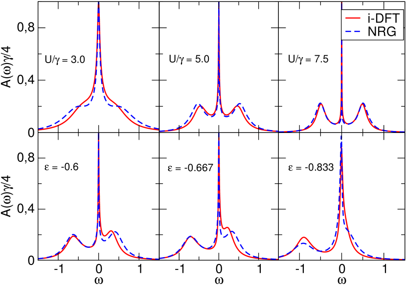
Figure 2: Comparison of Anderson model spectra calculated from i-DFT via Eq. (10) with NRG (taken from Ref. Motahari et al. (2016)). Upper panels: at the particle-hole symmetric point for different values of $U/\gamma$. Lower panels: for $U/\gamma=5$ at different values $\varepsilon$ for the on-site energy. Energies are given in units of $U$.

In Fig. 3 we show the i-DFT spectral functions for a degenerate 3-level CIM at various values of the gate. In most cases, the spectra are qualitatively similar to SIAM spectra. Only for $\varepsilon=-2$ (upper right panel) there is just a single spectral peak which essentially comes from one of the side peaks merging with the Kondo resonance as the position of the side peak changes from below to above the Fermi level as the gate is increased. We emphasize that the deviations of the i-DFT spectra from the exact ones have to be attributed entirely to the approximations we used for the Hxc gate and xc bias potentials. If their exact forms were used, the i-DFT spectra would be exact. We also note that the xc bias of Eq. (13) lends itself to straightforward generalization beyond the CIM by replacing $U$ with $U(K)\equiv\Delta_{\rm xc}(K)$ where we identified the charging energy $U(K)$ of charging state $K$ with the derivative discontinuity $\Delta_{\rm xc}(K)$ of the isolated dot with $K$ electrons. In this way it may be possible to construct an xc bias functional from a standard density functional provided the latter yields a non-vanishing derivative discontinuity Kraisler and Kronik (2013); Baer and Neuhauser (2005); Yamada et al. (2016).

In summary, we have proposed a computationally efficient DFT scheme to calculate the spectral function of an interacting many-electron system. Conceptually, this scheme allows to express the spectral function in terms of the ground state density (completely in line with the Hohenberg-Kohn theorem) although we use concepts from a DFT formulation for steady state transport (i-DFT). From the many-body spectral function one can obtain the many-body self-energy and the Green function which in our scheme therefore also allows to express them as functionals of the ground state density. In the derivation of our scheme and also in the applications shown here, we considered the typical transport setup of a system connected to two leads, one of them being the weakly coupled tip. However, the scheme should also be applicable to the calculation of surface and even bulk spectral functions by considering the system $S$ and the rest $R$ together while the tip just becomes a computational device to extract the spectral function. This idea as well as the corresponding construction of approximate functionals are subject of ongoing work.

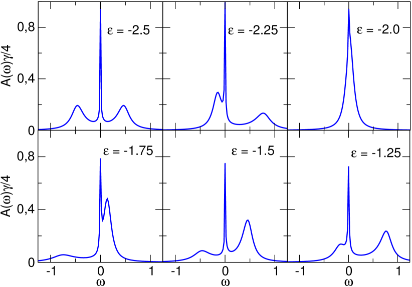
Figure 3: Spectral functions obtained from i-DFT for the CIM with three degenerate single-particle levels for $U/\gamma=8$ and different values of the gate potential. Energies in units of $U$.

References

- Hohenberg and Kohn (1964) P. Hohenberg and W. Kohn, Phys. Rev. 136, B864 (1964).
- Kohn and Sham (1965) W. Kohn and L. J. Sham, Phys. Rev. 140, A1133 (1965).
- Dreizler and Gross (1990) R. M. Dreizler and E. K. U. Gross, Density Functional Theory (Springer, Berlin, 1990).
- J.P. Perdew and Wang (1986) J.P. Perdew and Y. Wang, Phys. Rev. B 33, 8800 (1986), ibid. 40, 3399 (1989) (E).
- A.D. Becke (1988) A.D. Becke, J. Chem. Phys. 88, 1053 (1988).
- Lee et al. (1988) C. Lee, W. Yang, and R.G. Parr, Phys. Rev. B 37, 785 (1988).
- A.D. Becke (1993) A.D. Becke, J. Chem. Phys. 98, 5648 (1993).
- J.P. Perdew et al. (1996) J.P. Perdew, K. Burke, and M. Ernzerhof, Phys. Rev. Lett. 77, 3865 (1996), ibid. 78, 1396 (1997)(E).
- J.P. Perdew et al. (1999) J.P. Perdew, S. Kurth, A. Zupan, and P. Blaha, Phys. Rev. Lett. 82, 2544 (1999), ibid. 82, 5179 (1999)(E).
- Tao et al. (2003) J. Tao, J.P. Perdew, V.N. Staroverov, and G.E. Scuseria, Phys. Rev. Lett. 91, 146401 (2003).
- Kümmel and Kronik (2008) S. Kümmel and L. Kronik, Rev. Mod. Phys. 80, 3 (2008).
- Runge and E.K.U. Gross (1984) E. Runge and E.K.U. Gross, Phys. Rev. Lett. 52, 997 (1984).
- Ullrich (2012) C. Ullrich, Time-Dependent Density-Functional Theory (Oxford University Press, Oxford, 2012).
- Maitra (2016) N. T. Maitra, J. Chem. Phys. 144, 220901 (2016).
- Onida et al. (2002) G. Onida, L. Reining, and A. Rubio, Rev. Mod. Phys. 74, 601 (2002).
- Martin et al. (2016) R. Martin, L. Reining, and D. Ceperley, Interacting Electrons: Theory and Computational Approaches (Cambridge University Press, Cambridge, 2016).
- Capelle and Campo Jr. (2013) K. Capelle and V. L. Campo Jr., Phys. Rep. 528, 91 (2013).
- Stefanucci and Kurth (2015) G. Stefanucci and S. Kurth, Nano Lett. 15, 8020 (2015).
- Kurth and Stefanucci (2017) S. Kurth and G. Stefanucci, J. Phys.: Condens. Matter 29, 413002 (2017).
- Stefanucci and van Leeuwen (2013) G. Stefanucci and R. van Leeuwen, Nonequilibrium Many-Body Theory of Quantum Systems: A Modern Introduction (Cambridge University Press, Cambridge, 2013).
- Note (1) The non-interacting retarded and advanced GFs are independent of the bias by construction, while the lesser GF is in principle bias-dependent via the tip Fermi function : . However, in the limit the bias dependence vanishes as . As the interacting GFs can be written diagrammatically in terms of the non-interacting GFs and the electron-electron interaction does not depend on the bias either, it follows that the interacting GFs must also be independent of the bias in the limit , i.e. .
- Meir and Wingreen (1992) Y. Meir and N. S. Wingreen, Phys. Rev. Lett 68, 2512 (1992).
- Note (2) Transformation from symmetric voltage drop to a completely asymmetric voltage drop, and , is achieved by a spatially constant shift of the gate potential by , and subsequent substitution of the integration variable, .
- Anderson (1961) P. W. Anderson, Phys. Rev. 124, 41 (1961).
- Kurth and Stefanucci (2016) S. Kurth and G. Stefanucci, Phys. Rev. B 94, 241103(R) (2016).
- Perdew et al. (1982) J. P. Perdew, R. Parr, M. Levy, and J. L. Balduz, Phys. Rev. Lett. 49, 1691 (1982).
- Stefanucci and Kurth (2013) G. Stefanucci and S. Kurth, Phys. Stat. Sol. (b) 250, 2378 (2013).
- Bergfield et al. (2012) J. P. Bergfield, Z.-F. Liu, K. Burke, and C. A. Stafford, Phys. Rev. Lett. 108, 066801 (2012).
- Beenakker (1991) C. W. J. Beenakker, Phys. Rev. B 44, 1646 (1991).
- Stefanucci and Kurth (2011) G. Stefanucci and S. Kurth, Phys. Rev. Lett. 107, 216401 (2011).
- Tröster et al. (2012) P. Tröster, P. Schmitteckert, and F. Evers, Phys. Rev. B 85, 115409 (2012).
- Bulla et al. (2008) R. Bulla, T. A. Costi, and T. Pruschke, Rev. Mod. Phys. 80, 3950 (2008).
- Motahari et al. (2016) S. Motahari, R. Requist, and D. Jacob, Phys. Rev. B 94, 235133 (2016).
- Kraisler and Kronik (2013) E. Kraisler and L. Kronik, Phys. Rev. Lett. 110, 126403 (2013).
- Baer and Neuhauser (2005) R. Baer and D. Neuhauser, Phys. Rev. Lett. 94, 043002 (2005).
- Yamada et al. (2016) A. Yamada, Q. Feng, A. Hoskins, K. D. Fenk, and B. D. Dunietz, Nano Lett. 16, 6092 (2016), https://doi.org/10.1021/acs.nanolett.6b02241 .