On optimal control of free boundary
problems of obstacle type

Abstract

A numerical study of an optimal control formulation for a shape optimization problem governed by an elliptic variational inequality is performed. The shape optimization problem is reformulated as a boundary control problem in a fixed domain. The discretized optimal control problem is a non-smooth and non-convex mathematical programing problem. The performance of the standard BFGS quasi-Newton method and the BFGS method with the inexact line search are tested.

Keywords: obstacle problem, finite element method, shape optimization, non-smooth optimization

AMS subject classification: 49M37, 65N30, 90C30

1 Introduction

In the present paper a numerical method for shape optimization for a class of free boundary problems is proposed. The shape optimization problem is reformulated as a boundary control problem following the ideas discussed in [11]. The optimal shape is obtained as a level set. Thus, in numerical realization using finite elements, there is no need for remeshing during optimization iterations.

As a concrete free boundary (state) problem we consider the contact problem for the Poisson problem. In this case the free boundary is defined by the a-priori unknown contact zone. As a shape optimization problem we consider the problem of finding a shape having minimum area such that the contact zone includes a given subdomain [2].

It is well-known that in control problems for contact problems the control-to-state mapping is not smooth, in general. Despite this, many nonlinear programming codes for smooth optimization can be used to obtain reasonable approximate solutions to those control problems.

The paper is organized as follows. In Section 2 we present a shape optimization problem and an alternate boundary control formulation of it. Section 3 is devoted to disceretization and algebraic sensitivity analysis. Finally, a numerical study on the performance of two nonlinear programming codes applied to the discretized control problem is done in Section 4.

2 Setting of the problem

We consider an abstract shape optimization problem given formally as follows:

$$\left\{\begin{aligned} &\operatornamewithlimits{minimize}_{\alpha}F(\alpha,\Omega_{\alpha},y_{\alpha})\\ \text{subject to}&\\ &\text{Find }(\Omega_{\alpha},y_{\alpha}):\quad\mathcal{A}(\alpha,\Omega_{\alpha},y_{\alpha})=0.\end{aligned}\right.$$ (1)

Here $\alpha$ is the optimization (control) parameter, $\mathcal{A}$ represents a free boundary problem (in abstract operator form) whose solution consists both of the domain $\Omega_{\alpha}$ where the PDE is posed as well as the solution $y_{\alpha}$ to that PDE.

Problem (1) is more complicated than a classical shape optimization problem. In the latter the state problem is solved on a fixed domain, in the sense that $\Omega_{\alpha}$ is considered to be given instead of being one of the unknowns in the state problem.

Next we introduce the model problem to be studied in the rest of this paper. Let $\Omega\subset{\mathbb{R}}^{2}$ a domain, $f\in L^{2}(\Omega)$, $\psi\in C^{1}(\Omega)$. We consider the following classical free boundary problem: Find $(y_{\Omega},Z_{\Omega}),\ Z_{\Omega}{\subset}\Omega$ such that

$$\left\{\begin{aligned} -\Delta y_{\Omega}=f,\ y_{\Omega}>\psi&\quad\text{in }\Omega\setminus Z_{\Omega}\\ y_{\Omega}=0&\quad\text{on }\partial\Omega\\ y_{\Omega}=\psi&\quad\text{in }Z_{\Omega}\\ \frac{\partial{y_{\Omega}}}{\partial{n}}+\frac{\partial{\psi}}{\partial{n}}=0&\quad\text{on }\partial Z_{\Omega}.\end{aligned}\right.$$ (2)

Problem (2) models e.g. the contact between elastic membrane (represented by $\Omega$) and a rigid obstacle defined by $\psi$. The solution $y_{\Omega}$ to (2) then gives the vertical displacement of the membrane under the vertical load represented by $f$. The set $Z_{\Omega}$ is the contact zone between the membrane and the obstacle.

Problem (2) can be formulated as the following variational inequality ([6]):

$$y_{\Omega}\in K_{0}(\Omega):\quad\int_{\Omega}\nabla y_{\Omega}\cdot\nabla(w{-}y_{\Omega})\,dx\geq\int_{\Omega}f(w-y_{\Omega})\,dx\quad w\in K_{0}(\Omega),$$ (3)

where

$$K_{g}(D):=\left\{v\in H^{1}(D)\mid v{\geq}\psi\text{ in }D\text{ and }v{=}g\text{ on }\partial D\right\}.$$

This formulation does not include explicitly the contact zone $Z_{\Omega}$ as an unknown.

Let ${\widehat{\Omega}}\subset{\mathbb{R}}^{2}$ and $\Omega_{0}\subset{\mathbb{R}}^{2}$ be given bounded domains such that $\Omega_{0}\subsetneq{\widehat{\Omega}}$. We introduce a system of bounded domains

$${\mathcal{O}}=\{\Omega\subset{\widehat{\Omega}}\mid\Omega\text{ has Lipschitz boundary}\}.$$

Let $y_{\Omega}$ be the unique solution to (3) and let $C(y_{\Omega})=\{x\in\Omega\mid y_{\Omega}(x)=\psi(x)\text{ a.a. }x\}$ denote the corresponding contact region. We consider the following shape optimization problem introduced in [2]:

$$\left\{\begin{aligned} &\operatornamewithlimits{minimize}_{\Omega\in{\mathcal{O}}}\ \mathcal{J}(\Omega)=\int_{\Omega}\,dx\\ &\text{subject to \eqref{eq:VI} and }\Omega_{0}\subset C(y_{\Omega}).\end{aligned}\right.$$ (4)

We are thus looking for a domain $\Omega^{\star}$ (representing the membrane) having minimum area such that the contact region ”covers” the given domain $\Omega_{0}$.

The state constraint $\Omega_{0}\subset C(y_{\Omega})$ can be relaxed by introducing a penalty term resulting in the shape optimization problem

$$\left\{\begin{aligned} &\operatornamewithlimits{minimize}_{\Omega\in{\mathcal{O}}}\quad\mathcal{J}_{\varepsilon}(\Omega)=\int_{\Omega}\,dx+\frac{1}{{\varepsilon}}\int_{\Omega_{0}}(y_{\Omega}-\psi)^{2}\,dx\\ &\text{subject to \eqref{eq:VI}},\ {\varepsilon}>0.\end{aligned}\right.$$ (5)

One of the main difficulties in the theoretical and numerical treatment of the problem (5) consists in the variable character of the domain $\Omega$ on which the state problem (3) is given. Theoretical and numerical aspects of shape optimization using ”moving” domains are discussed e.g. in refs [12], [13], [8], [7].

Alternatively, there has been significant amount of interest in fixed domain formulations of shape optimization problems (see e.g. [5]). The most common approaches to get rid of moving domains are the following:

• By scaling the domain such that it becomes fixed, the optimization parameter appears as a coefficient in the state problem.

• The domain $\Omega$ is represented by a level set $\Omega=\{x\in{\widehat{\Omega}}\mid\Phi(x)<0\}$, where $\Phi:{\widehat{\Omega}}\to{\mathbb{R}}$ is an unknown level set function to be determined.

• The state problem is modified by adding control variable to it. An optimal shape is defined implicitly by a level set (but without separate level set function).

Boundary control approach

In this paper we utilize the boundary control approach discussed in [11]. In what follows we assume that $f\leq 0$ and $\psi<0$. We define the set of admissible controls as follows

$${\mathcal{U}}=\{u:\partial{\widehat{\Omega}}\to{\mathbb{R}}\mid u\in C(\partial{\widehat{\Omega}}),\ u_{\min}\leq u\leq u_{\max}\},$$

where $u_{\min},u_{\max}>0$ are given constants. Next, to each $u\in{\mathcal{U}}$ we associate $y(u)$, the solution to the variational inequality

$$\left\{\begin{aligned} &\text{Find }y(u)\in K_{u}({\widehat{\Omega}})\text{ such that}\\ &\int_{\widehat{\Omega}}\nabla y(u)\cdot\nabla(w{-}y(u))\,dx\geq\int_{\widehat{\Omega}}f(w{-}y(u))\,dx\quad\forall w\in K_{u}({\widehat{\Omega}}).\end{aligned}\right.$$ (6)

Let $H:{\mathbb{R}}\to{\mathbb{R}}$ denote the Heaviside step function. We consider the following boundary control problem posed in a fixed domain:

$$\left\{\begin{aligned} &\operatornamewithlimits{minimize}_{u\in{\mathcal{U}}}\ J_{\varepsilon}(u)=\int_{{\widehat{\Omega}}}\bigl{(}1-H(y(u))\bigr{)}\,dx+\frac{1}{{\varepsilon}}\int_{\Omega_{0}}(y(u)-\psi)^{2}\,dx\\ &\text{subject to \eqref{eq:VI2}}.\end{aligned}\right.$$ (7)

As $u>0$ on $\partial{\widehat{\Omega}}$ and $f\leq 0,\psi<0$ in ${\widehat{\Omega}}$ it follows that for suitable choice of $u$ the set of points where $y(u)$ is strictly negative is non-empty. The first term in the cost functional $J_{\varepsilon}$ gives the area of this set while the latter term adds a penalty if the contact zone $C(y(u))$ does not cover $\Omega_{0}$.

Assume that there exists an optimal pair $(u^{\star}_{\varepsilon},y^{\star}_{\varepsilon}):=({u_{\varepsilon}^{\star}},y({u_{\varepsilon}^{\star}}))$ for (7). We can now consider $\Omega_{\varepsilon}^{\star}:=\{x\in{\widehat{\Omega}}\mid y^{\star}_{\varepsilon}(x)<0\}$ as an approximate solution to the original shape optimization problem (4).

The control approach clearly makes sense if $\Omega_{0}$ is simple enough star-like domain. If, however, $\Omega_{0}$ is e.g. multiply connected the set $\Omega_{\varepsilon}^{\star}$ might not approximately solve (5).

3 Approximation and numerical realization

To realize (7) numerically, we must discretize both the control and state variables. In what follows, we assume that ${\widehat{\Omega}}$ is the disk $B(0,R)$. We discretize the state problem (6) by using piecewise linear triangular elements. Instead of the exact Heaviside function, we use the smoothed one

$$H_{\beta}(x):=\tfrac{1}{2}\tanh(\tfrac{x}{\beta})+\tfrac{1}{2},\quad\beta>0.$$

The use of piecewise linear triangular elements implies that the most obvious way to discretetize the control $u$ would be to use piecewise linear and continuous discretization in the same finite element mesh where the state variable is discretized. However, this approach has two well-known drawbacks. Firstly, the number of optimization variables is very large whenever dense meshes are used. Secondly, the piecewise linear approximation (without a suitable regularization term in the cost function) is prone to spurious oscillations.

Instead, we look for a differentiable and periodic function $u_{\boldsymbol{a}}:[0,2\pi]\to{\mathbb{R}}$ that is fully defined by a vector of parameters ${\boldsymbol{a}}=(a_{1},a_{2},...,a_{n})$. Examples of such functions are Bezier functions, cubic Hermite, and cubic spline interpolating polynomials, e.g.

Here we shall use shape preserving periodic piecewise cubic Hermite interpolation polynomial (see [4], [1]) to represent the control function. The parametrized control function solves the following interpolation problem

$$u_{\boldsymbol{a}}\in C^{1}([0,2\pi]),\quad u^{\prime}_{\boldsymbol{a}}(0-)=u_{\boldsymbol{a}}^{\prime}(2\pi+)$$

$$u_{\boldsymbol{a}}(0){=}a_{1},\ u_{\boldsymbol{a}}(\Delta){=}a_{2},...,u_{\boldsymbol{a}}(2\pi{-}\Delta){=}a_{n},\ u_{\boldsymbol{a}}(2\pi){=}a_{1}.$$

The advantage of this kind of parametrization is that the number of discrete optimization variables is small but at the same time the control is a smooth function without excessively prone to wild oscillations. Moreover, the interpolant $u_{\boldsymbol{a}}$ does not overshoot the data, so $u_{\boldsymbol{a}}\in{\mathcal{U}}$ if $u_{\min}\leq a_{i}\leq u_{\max}\ \forall i$.

Sensitivity analysis for the discrete state problem

Let $\mathcal{I}=\{1,...,N\}$ denote the set of node numbers in the finite element model and let $\mathcal{I}_{d}\subset\mathcal{I}$ be the node numbers of the boundary nodes. Let $\boldsymbol{\psi}=\{\psi_{1},...,\psi_{N}\}$ be the vector of nodal values of the obstacle and let ${\boldsymbol{u}}=\{u_{i_{1}},...,u_{i_{m}}\}$ be the vector of nodal values of the boundary control. Then the finite element approximation of the variational inequality (6) can be expressed as an equivalent quadratic programming problem

$$\left\{\begin{aligned} &\operatornamewithlimits{minimize}_{{\boldsymbol{q}}}\ \Pi({\boldsymbol{q}})=\tfrac{1}{2}{{\boldsymbol{q}}}^{\text{T}}{\boldsymbol{K}}{\boldsymbol{q}}-{{\boldsymbol{f}}}^{\text{T}}{\boldsymbol{q}}\\ &\text{subject to}\quad q_{i}{=}u_{\boldsymbol{a}}(x_{i}),\ i\in\mathcal{I}_{d},\quad q_{i}{\geq}\psi_{i},\ i\in\mathcal{I}\setminus\mathcal{I}_{d},\end{aligned}\right.$$ (8)

where ${\boldsymbol{K}}$ and ${\boldsymbol{f}}$ are the stiffness matrix and the force vector, respectively.

The discretization of the boundary control problem (7) leads to the nonlinear programming problem

$$\left\{\begin{aligned} &\operatornamewithlimits{minimize}_{{\boldsymbol{a}}}J_{\varepsilon}({\boldsymbol{a}})\\ &\text{subject to }\eqref{eq:QP}\text{ and }u_{\min}\leq a_{k}\leq u_{\max},\ k=1,...,n.\end{aligned}\right.$$ (9)

To be able to use descent type optimization methods we need to evaluate the gradient of $J_{\varepsilon}$ with respect to the discrete control variable ${\boldsymbol{a}}$.

Let $\mathcal{I}_{c}({\boldsymbol{a}})$ denote the set of contact nodes, i.e. the solution ${\boldsymbol{q}}={\boldsymbol{q}}({\boldsymbol{a}})$ satisfies $q_{i}=\psi_{i},\ i\in\mathcal{I}_{c}({\boldsymbol{a}})$. Let $\widetilde{{\boldsymbol{a}}}$ be the current approximation of the optimal control. If we assume that $\mathcal{I}_{c}(\widetilde{{\boldsymbol{a}}})$ is known a priori and it is invariant under small perturbations of $\widetilde{{\boldsymbol{a}}}$, then $J$ is differentiable and the gradient $\nabla_{\boldsymbol{a}}J_{\varepsilon}(\widetilde{{\boldsymbol{a}}})$ can be obtained using the standard adjoint equation technique. However, if the contact set changes due to arbitrary small perturbation, the mapping ${\boldsymbol{a}}\mapsto J_{\varepsilon}({\boldsymbol{a}})$ is not differentiable at $\widetilde{{\boldsymbol{a}}}$ and the mechanical application of the adjoint technique gives at most an element from the subdifferential.

Additional source of nonshmoothness

Consider piecewise cubic Hermite interpolation of the data $(x_{1},y_{1})$, $(x_{2},y_{2}),....,(x_{n},y_{n})$. On each subinterval $[x_{k},x_{k+1}]$ the interpolant can be expressed in terms of a local variable $s=x-x_{k}$ as follows

$$p(x)=\frac{3hs^{2}-2s^{3}}{h^{3}}y_{k+1}+\frac{h^{3}-3hs^{2}+2s^{3}}{h^{3}}y_{k}+\frac{s^{2}(s-h)}{h^{2}}d_{k+1}+\frac{s(s-h)^{2}}{h^{2}}d_{k}.$$

The interpolant satisfies the following interpolation conditions

$$p(x_{k})=y_{k},\ p^{\prime}(x_{k})=d_{k},\ p(x_{k+1})=y_{k+1},\ p^{\prime}(x_{k+1})=d_{k+1}.$$

In the classical piecewise cubic Hermite interpolation, the slope parameters $d_{k},\ k=1,...,n$ are a priori given constants.

In shape-preserving piecewise cubic interpolation, the slopes are not supplied by the user. Instead, they are computed algorithmically as a part of the interpolating process in the following way: Let $\delta_{k}=(y_{k+1}-y_{k})/(x_{k+1}-x_{k})$ and $h_{k}=x_{k+1}-x_{k}$. The slopes $d_{k}$ are determined as follows. If $\text{sign}(\delta_{k})\cdot\text{sign}(\delta_{k-1})<0$ we set $d_{k}=0$. If $\text{sign}(\delta_{k})\cdot\text{sign}(\delta_{k-1})>0$ and the two intervals have the same length, then $d_{k}$ is the harmonic mean of $\delta_{k-1}$ and $\delta_{k}$:

$$\frac{1}{\delta_{k}}=\tfrac{1}{2}\left(\frac{1}{\delta_{k-1}}+\frac{1}{\delta_{k}}\right).$$

If the intervals have different lengths, then $d_{k}$ is the following weighted harmonic mean

$$\frac{w_{1}+w_{2}}{d_{k}}=\frac{w_{1}}{\delta_{k-1}}+\frac{w_{2}}{\delta_{k}},$$

where $w_{1}=2h_{k}+h_{k-1}$, $w_{2}=h_{k}+2h_{k-1}$.

The advantage of shape-preserving piecewise cubic interpolation over cubic spline interpolation is that the interpolant does not overshoot the data.

Consider next the case where the vector of values ${\boldsymbol{y}}=(y_{1},...,y_{n})$ is an optimization parameter. In case of cubic spline interpolation, the vector of slopes is obtained by solving a tridiagonal system ${\boldsymbol{A}}{\boldsymbol{d}}={\boldsymbol{b}}$, where the vector ${\boldsymbol{b}}$ is a linear function of ${\boldsymbol{y}}$. Thus the value of the interpolant at given fixed point $x$ is a smooth function of ${\boldsymbol{y}}$.

With shape-preserving piecewise cubic interpolation the situation is different. The mapping ${\boldsymbol{y}}\mapsto{\boldsymbol{d}}$ is clearly nonlinear. In addition, it is nonsmooth. A simple example shown in Figure 1 demonstrates this.

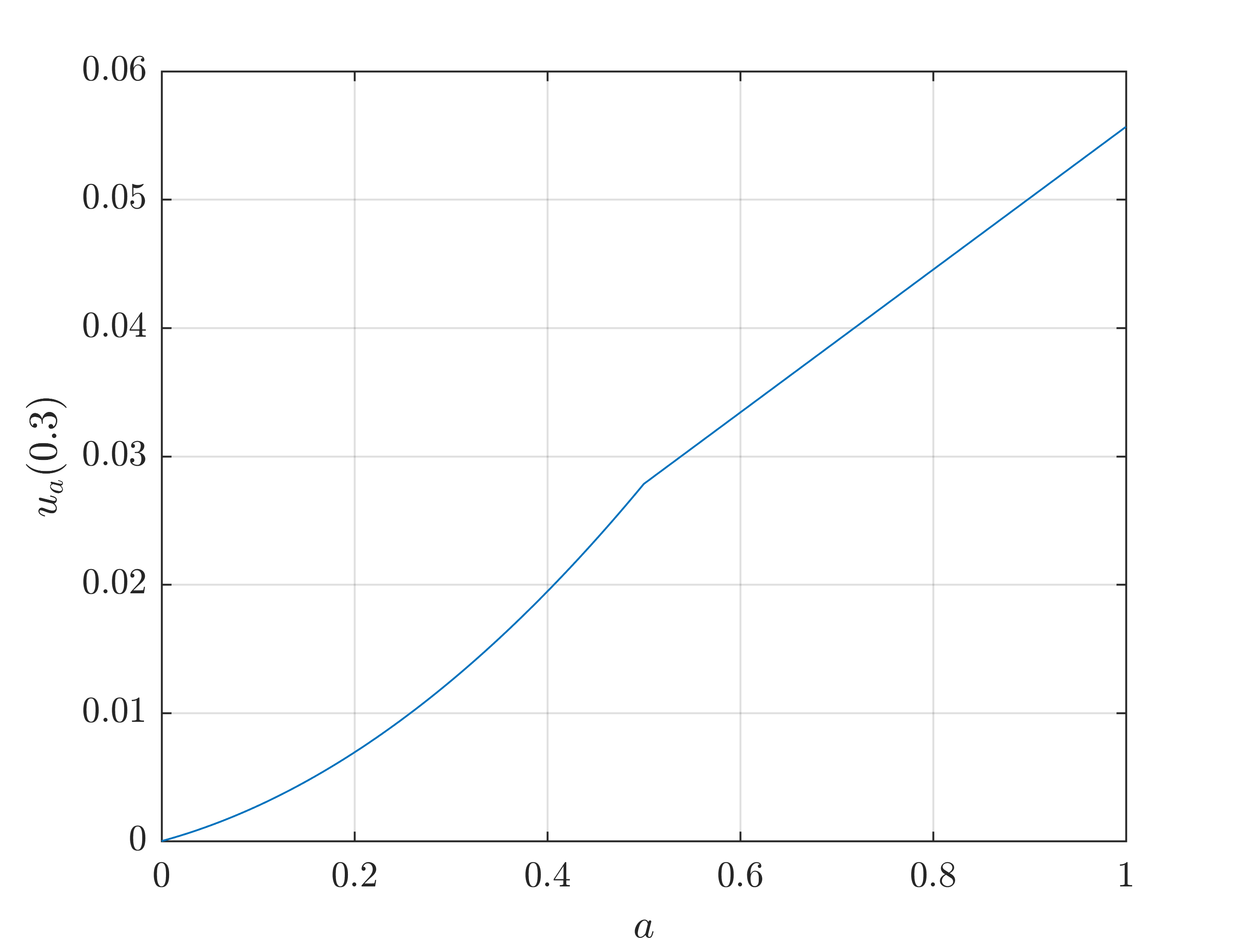
Figure 1: Periodic shape-preserving piecewise cubic Hermite interpolation of the data ${\boldsymbol{x}}{=}(0,\tfrac{2\pi}{3},\tfrac{4\pi}{3},2\pi),\ {\boldsymbol{y}}{=}(0,a,\tfrac{1}{2},0)$. The value of the interpolant $u_{a}(x)$ at $x{=}0.3$ is plotted against the parameter $a$.

4 Numerical examples

In this section we present two numerical examples. All finite element computations are implemented in Matlab [10]. The quadratic programming problem (8) is solved using Matlab’s quadprog function. The box constraints $u_{\min}\leq a_{i}\leq u_{\max}$ are implemented by adding a smooth penalty function

$$\tfrac{\gamma}{2}\sum_{i=1}^{n}\left[(a_{i}-u_{\max})_{+}^{2}+(u_{\min}-a_{i})_{+}^{2}\right]$$

with $\gamma=10^{-3}$ to the cost function.

The optimal control problem is solved by using two different optimizers:

• Function fminunc from Matlab’s Optimization Toolbox with ’quasi-newton’ option that implements the standard BFGS method.

• Optimizer HANSO 2.2 (Hybrid Algorithm for Non-Smooth Optimization [3], [9]) that implements BFGS method with inexact line search.

For the options of fminunc that control the optimality tolerance we use their default values. Also we use the default options of HANSO. Especially, we do not use the option available in HANSO to continue the optimization using the gradient sampling method as this option is very expensive in terms of the number of function evaluations.

In all examples we use the following parameter values. The radius defining the computational domain $\hat{\Omega}$ is $R=1.75$. The right hand side function $f\equiv-10$ and the obstacle $\psi(x)=-0.3\left(x_{1}^{2}+(x_{2}{-}0.25)^{2}\right)-0.05$. The target domain $\Omega_{0}$ to be covered is the isosceles triangle with vertices $({-}1,0)$, $(\tfrac{1}{2},\tfrac{3}{4})$, $(\tfrac{1}{2},{-}\tfrac{3}{2})$ The parameters defining ${\mathcal{U}}$ are $u_{\min}{=}0.01$ and $u_{\max}{=}10$. The Heaviside smoothing parameter is $\beta{=}10^{-3}$ and penalty parameter is ${\varepsilon}=10^{-3}$.

Example 1.

Here we use an unstructured finite element mesh with nominal mesh size $h=0.05$. The mesh is constructed in such way that $\partial\Omega_{0}$ coincides element edges.

We ran both optimizers using $n=30$ and $a_{i}^{(0)}{=}2,\ i{=}1,...,n$ until they were not able to improve the control. The evolution of the best objective value versus computational work is depicted for both methods in Figure 2. The implicitly defined optimized domains $\Omega_{\varepsilon}^{\star}$ (with the corresponding contours of $y_{\varepsilon}^{\star}$) and the optimal boundary controls are plotted in Figures 3 and 4.

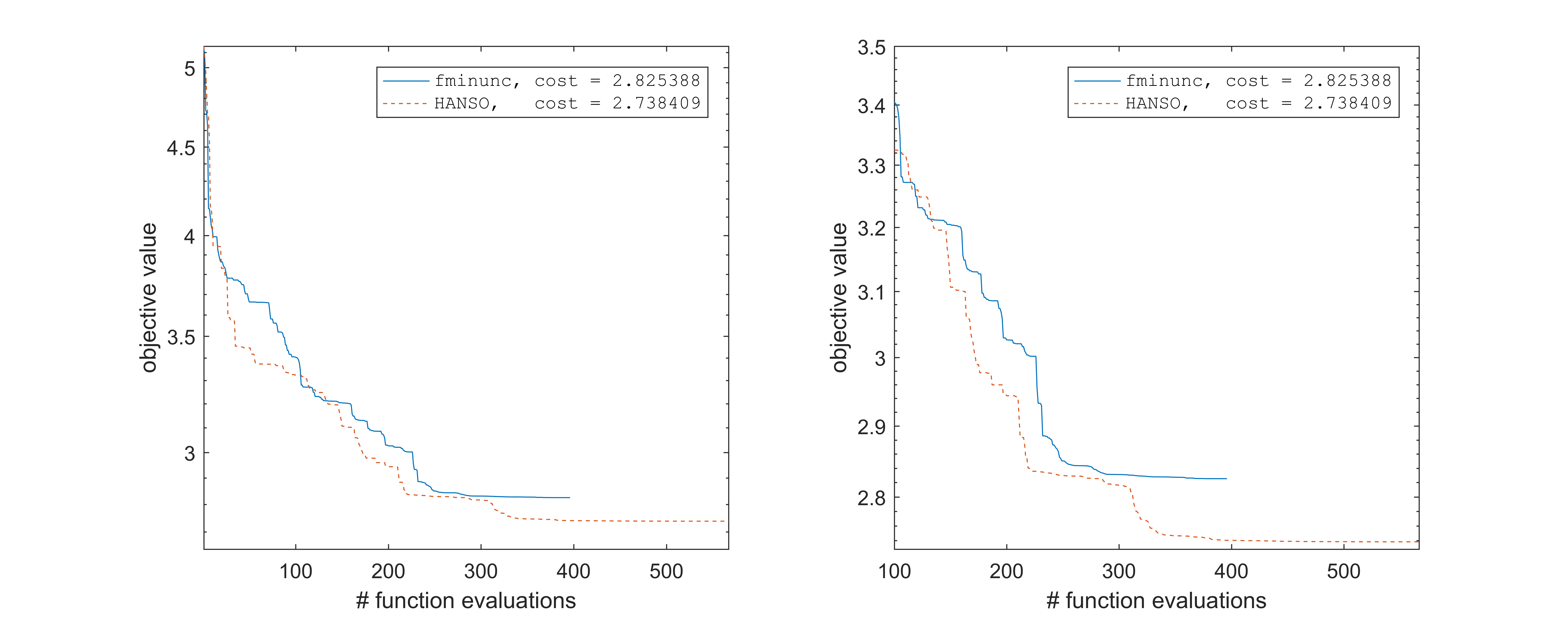
Figure 2: Best objective value versus the number of function evaluations

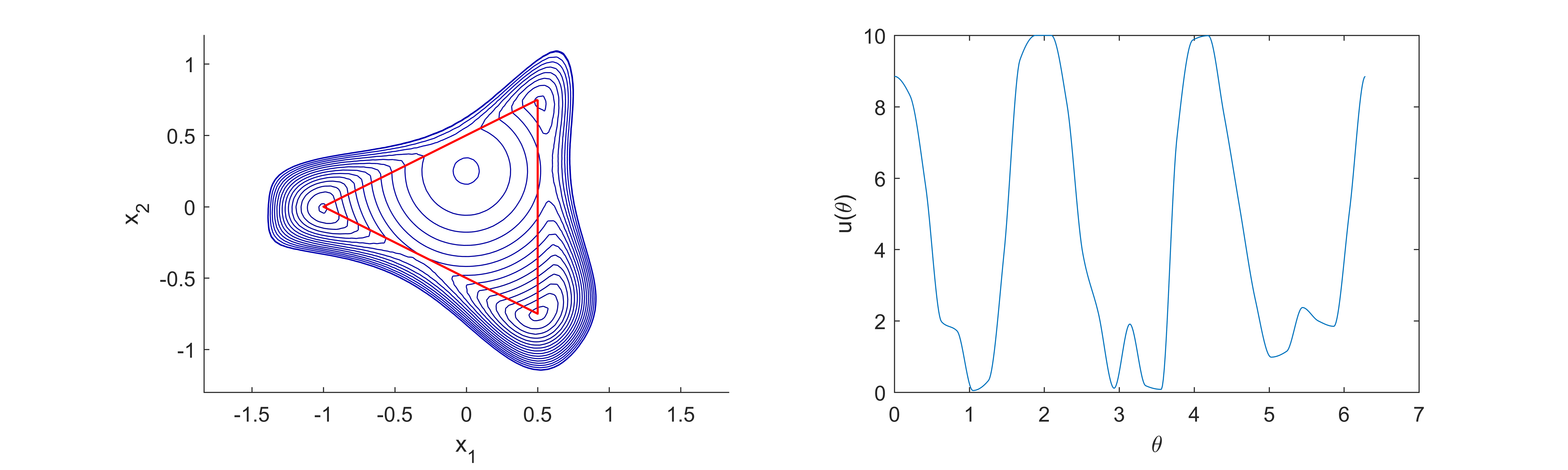
Figure 3: Optimized domain (left) and control (right) computed using fminunc. The boundary of the target contact zone $\Omega_{0}$ is depicted as the red triangle.

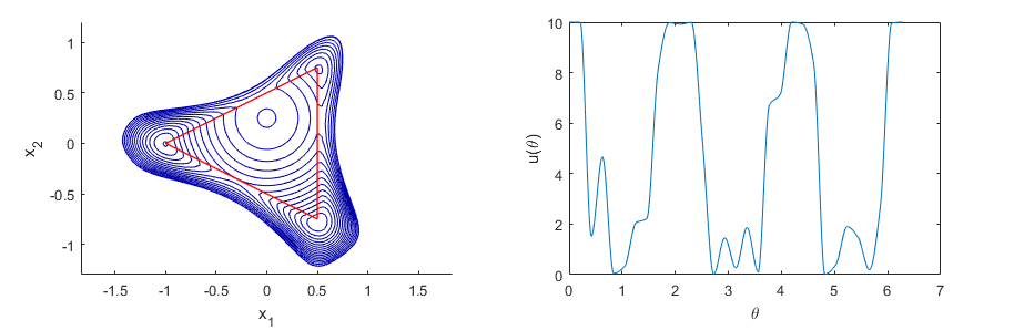
Figure 4: Optimized domain (left) and control (right) computed using HANSO 2.2

One can observe that in this example HANSO 2.2 finds better control than fminunc. However, HANSO 2.2 spends considerable amount of computational work with only very marginal improvement in the cost function.

Example 2.

In this example the mesh is generated in the same way as in Example 1 except the nominal mesh size is $h=0.025$. The evolution of the best objective value versus computational work is depicted for both methods in Figure 5. The implicitly defined optimized domains $\Omega_{\varepsilon}^{\star}$ (with the corresponding contours of $y_{\varepsilon}^{\star}$) and the optimal boundary controls are plotted in Figures 6 and 7.

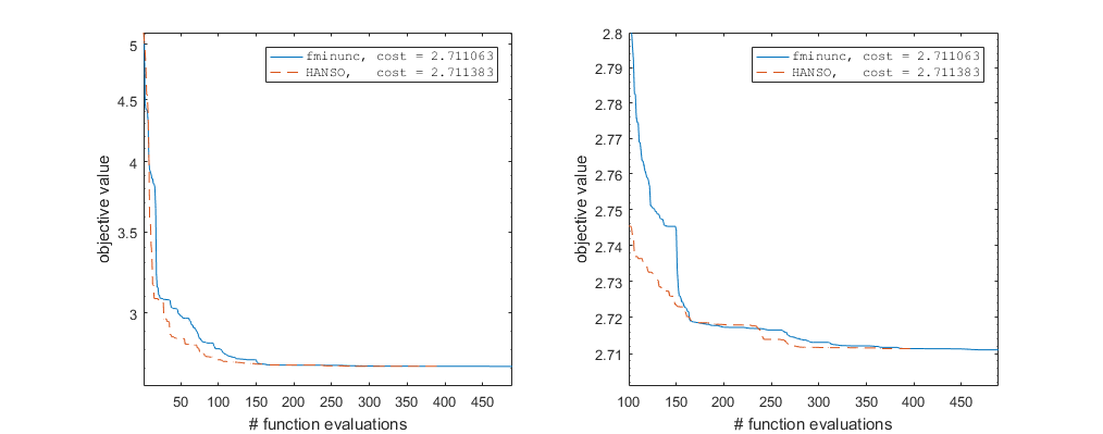
Figure 5: Best objective value versus the number of function evaluations

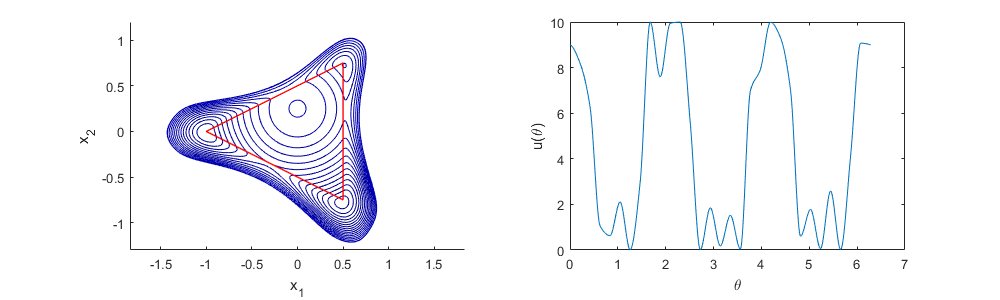
Figure 6: Optimized domain (left) and control (right) computed using fminunc

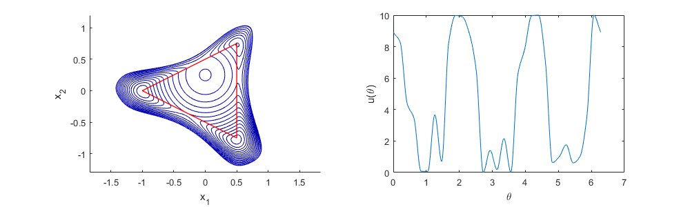
Figure 7: Optimized domain (left) and control (right) computed using HANSO 2.2

This time both optimizers end up to almost same final objective value using essentially same amount of computational work. However, the optimized controls and the corresponding domains $\Omega_{\varepsilon}^{\star}$ differ considerably.

The results of Examples 1 and 2 show that the method works reasonably well. The obtained shapes are approximately feasible (due to penalization) and the objective function value was substantially reduced. However, there is no guarantee that any of the obtained domains is even a local minimizer.

From the results, we can also deduce that the boundary control problem is ill-conditioned. The effect of ill-conditioning can be seen by comparing the optimized controls obtained by using the two different optimizers. Comparing the convergence history we see that significant differences in the details of the boundary control have only a minor effect on the value of the objective function. This is due to the fact that the solution of the Poisson problem is generally smoother than the data. Similar stiffness appears e.g. in identification problem related to the Bernoulli free boundary problem studied in [14].

5 Conclusions

In this paper we have considered some computational aspects of a shape optimization problem with the state constraint given by a free boundary/obstacle problem. The free boundary problem is formulated as a quadratic programming problem which is then solved using the state-of-the-art tools. To solve the optimal shape design problem, a boundary control approach was used. Its main advantage is that there is no need to consider moving domains. This is advantageous especially from the computational point of view.

A well-known feature of optimal control problems governed by obstacle type problems is that the control-to-state mapping is not smooth in general. However, in discrete setting, it is piecewise smooth. In those points where it is smooth, the gradient of the objective function can be evaluated in a straightforward way using the adjoint approach.

Numerical examples show that the location of the boundary of the contact zone can be adjusted by changing the boundary control. However, it seems that the problem is ill-conditioned in the sense that relatively large changes in the boundary control have only a little effect on the location of the contact zone boundary. We did not make a detailed trade-off study between accuracy and oscillations. That will be a topic in further studies. One possible remedy (and a topic for further studies) would be to consider distributed control instead of boundary control as was also done in [11].

References

- [1] J. Bastien, Periodical cubic interpolation, version 1.1. https://mathworks.com/matlabcentral/fileexchange/46580, 2014. Accessed: 2017-12-12.
- [2] B. Benedict, J. Sokolowski, and J. P. Zolesio, Shape optimization for the contact problems, in 11th IFIP Conference on System Modelling and Optimization, P. Topft-Christia¡rsen, ed., vol. 59 of Lecture Notes in Control and Inform. Sciences, Springer-Verlag, 1984, pp. 789–799.
- [3] J. V. Burke, A. S. Lewis, and M. L. Overton, A robust gradient sampling algorithm for nonsmooth, nonconvex optimization, SIAM J. Optimization, 15 (2005), pp. 751–779.
- [4] F. N. Fritsch and R. E. Carlson, Monotone piecewise cubic interpolation, SIAM J. Numerical Analysis, 17 (1980), pp. 238–246.
- [5] P. Fulmański, A. Laurain, J.-F. Scheid, and J. Sokołowski, A level set method in shape and topology optimization for variational inequalities, Int. J. Appl. Math. Comput. Sci, 17 (2007), pp. 413–430.
- [6] R. Glowinski, Numerical Methods for Nonlinear Variational Problems, Springer Series in Computational Physics, Springer-Verlag, New York, Berlin, Heidelberg, Tokyo, 1984.
- [7] J. Haslinger and R. A. E. Mäkinen, Introduction to Shape Optimization: Theory, Approximation, and Computation, Society for Industrial and Applied Mathematics, Philadelphia, PA, 2003.
- [8] J. Haslinger and P. Neittaanmäki, Finite element approximation for optimal shape, material, and topology design, John Wiley & Sons, 1996.
- [9] A. S. Lewis and M. L. Overton, Nonsmooth optimization via quasi-Newton methods, Math. Program., 141 (2013), pp. 135–163.
- [10] MATLAB, Release R2016b with Optimization Toolbox 7.5, The MathWorks Inc., Natick, Massachusetts, 2016.
- [11] P. Neittaanmäki and D. Tiba, An embedding of domains approach in free boundary problems and optimal design, SIAM J. Control and Optimization, 33 (1995), pp. 1587–1602.
- [12] O. Pironneau, Optimal Shape Design for Elliptic Systems, Springer Series in Computations Physics, Springer Verlag, 1984.
- [13] J. Sokołowski and J.-P. Zolesio, Introduction to Shape Optimization, Springer Verlag, 1992.
- [14] J. I. Toivanen, J. Haslinger, and R. A. E. Mäkinen, Shape optimization of systems governed by bernoulli free boundary problems, Computer Methods in Applied Mechanics and Engineering, 197 (2008), pp. 3803–3815.